Late Time Quantum Chaos of pure states in the SYK model

Abstract

In this letter, we study the return amplitude, which is the overlap between the initial state and the time evolved state, in the Sachdev-Ye-Kitaev (SYK) model. Initial states are taken to be product states in a spin basis. We numerically study the return amplitude by exactly diagonalizing the Hamiltonian. We also derive the analytic expression for the return amplitude in random matrix theory. The SYK results agree with the random matrix expectation. We also study the time evolution under the different Hamiltonian that describes the traversable wormholes in projected black holes in the context of holography. The time evolution now depends on the choice of initial product states. The results are again explained by random matrix theory. In the symplectic ensemble cases, we observed an interesting pattern of the return amplitude where they show the second dip, ramp and plateau like behavior.

1.Introduction The Sachdev-Ye-Kitaev (SYK) modelPhysRevLett.70.3339 ; KitaevTalk is an interesting model. This model is solvable at large $N$Maldacena:2016hyu ; Kitaev:2017awl but maximally chaoticKitaevTalk ; Maldacena:2015waa , shows random matrix behaviors PhysRevB.95.115150 ; Cotler:2016fpe , and shares the same sector with two dimensional dilaton gravityJACKIW1985343 ; Teitelboim:1983ux ; Almheiri:2014cka ; Maldacena:2016upp .

In this letter, we study the time dependence of pure states in the SYK model. Here we consider a special class of pure states that were first considered in Kourkoulou:2017zaj ; Krishnan:2017txw and studied further in Hunter-Jones:2017raw ; Dhar:2018pii ; Bhattacharya:2018fkq . They are simultaneous eigenstates of spin operators that are constructed from Majorana fermions. One interesting physical interpretation of these states is that they are states after projection measurements of maximally entangled states by these spin operatorsKourkoulou:2017zaj ; Numasawa:2016emc . In this context, we can interpret our setup as time evolution after projection measurements. We expect that the time evolution starts flipping these spins under the SYK Hamiltonian and we get a more general superpositions of these product states. In this paper, we consider the return amplitude, which is the square of the fidelity and used in the similar setup in conformal field theoryCardy:2014rqa ; Cardy:2016lei . We can also consider the time evolution under deformed Hamiltonians after the measurements. Here we consider a deformation proposed by Kourkoulou:2017zaj . They are interpreted as a traversable wormhole protocol to see the inside of black holesKourkoulou:2017zaj ; Brustein:2018fkr . This deformed Hamiltonian can also be seen as deformation of an integrable Hamiltonian with degenerate spectrum by the chaotic SYK Hamiltonian.

2.The SYK Model In the SYK model, we consider even $N$ Majorana fermions $\psi_{i}$ that are obeyed to the anti commutation relation $\{\psi_{i},\psi_{j}\}=\delta_{ij}$. The Hamiltonian of the SYK model with $q$ body interactions is given by

$$H_{SYK}=i^{{q\over 2}}\sum_{a_{1}<a_{2}<\cdots<a_{q}}J_{a_{1}\cdots a_{q}}\psi_{a_{1}}\cdots\psi_{a_{q}}.$$ (1)

Here $J_{a_{1}\cdots a_{q}}$ are random couplings with mean $\braket{J_{a_{1}\cdots a_{q}}}_{J}=0$ and variance $\braket{J_{a_{1}\cdots a_{q}}^{2}}_{J}={J^{2}(q-1)!\over N^{q-1}}$. The $q=4$ model is the original SYK model that we mainly focus on in this letter. This system has two important symmetriesPhysRevB.95.115150 PhysRevB.83.075103 . The first one is the anti unitary symmetry $\mathcal{T}$. This symmetry satisfies $\mathcal{T}\psi_{a}\mathcal{T}^{-1}=\psi_{a}$. The SYK Hamiltonian (1) is invariant under $\mathcal{T}$ when $q=0\ (\text{mod}\ 4)$. The other important symmetry is the mod $2$ fermion number operator $(-1)^{F}$ with $((-1)^{F})^{2}=1$. These symmetries can have global anomalies depending on $N$ (mod $8$)PhysRevB.83.075103 . These anomalies are the origin to realize all of Gaussian unitary (GUE), orthogonal (GOE) and symplectic (GSE) ensembles in the SYK modelPhysRevB.95.115150 . Here we summarize the resultsPhysRevB.95.115150 ; Kanazawa:2017dpd in the table.1.

Table 1: symmetry property in the SYK model

$N\ (\text{mod}\ 8)$	$\mathcal{T}^{2}$	$\mathcal{T}(-1)^{F}=a(-1)^{F}\mathcal{T}$	statistics	degeneracy
$N=0$	$+1$	$a=+1$	GOE	1
$N=2$	$+1$	$a=-1$	GUE	2
$N=4$	$-1$	$a=+1$	GSE	2
$N=6$	$-1$	$a=-1$	GUE	2

Now, we consider the return amplitude. The return amplitude is

$$g_{p}(t)=|\bra{\psi_{0}}e^{-iHt}\ket{\psi_{0}}|^{2}.$$ (2)

Here $\ket{\psi_{0}}$ is a initial state and $H$ is the Hamiltonian of the system. This definition is also applicable to any quantum systems. We take the square of $|\bra{\psi_{0}}e^{-iHt}\ket{\psi_{0}}|$, which is different from the definition in Cardy:2014rqa ; Cardy:2016lei . Our choice makes the relation to so called spectral form factor clear, which is studied extensively in the field of quantum chaos and also recently in holographyCotler:2016fpe ; Balasubramanian:2016ids ; Benjamin:2018kre ; Chenu:2018spm ; delCampo:2017bzr .

Because we expect that the late time behavior of the SYK model is governed by random matrices Cotler:2016fpe , it is good to study first the return amplitude in random matrix theory. Now we want to compute $\braket{}{\bra{\psi_{0}}e^{-iHt}\ket{\psi_{0}}}{{}^{2}}_{\text{GUE}}=\int dHe^{-{L\over 2}\text{Tr}H^{2}}|\bra{\psi_{0}}e^{-iHt}\ket{\psi_{0}}|^{2}$ where $dH$ is the Haar measure on the space of $L\times L$ Hermitian matrices. We can compute this in random matrix theory using the Haar integrals. The results are

$$\braket{}{\bra{\psi_{0}}e^{-iHt}\ket{\psi_{0}}}{{}^{2}}_{\text{GUE}}={1\over L(L+1)}(\braket{g(t)}_{\text{GUE}}+L),$$ (3)

where $g(t)=Z(t)Z(t)^{*}$ with $Z(t)=\text{Tr}(e^{-iHt})$. This $g(t)$ is the spectral form factor, which diagnoses the energy level correlations in chaotic systems. We also find that this relation also holds in GSE ensemble by replacing the aevrage to $\braket{}_{GSE}$, using the Haar integral2006CMaPh.264..773C ; 1997PhRvB..55.1142A . In GOE ensemble, the return amplitude depends on the initial state $\ket{\psi_{0}}$. The equation (3) means that the return amplitude is given essentially by the constant $L$ shift of the spectral form factor. When $t=0$, the spectral form factor is simply given by the square of the dimension of the Hilbert space $g(0)=L^{2}$. Under the time evolution, $\braket{g(t)}_{\text{GUE}}$ decreases and hit the minimal value. These regimes are called the slope and the dip Cotler:2016fpe . Then, $\braket{g(t)}_{\text{GUE}}$ increases linearly. This linear growth is called the rampCotler:2016fpe and this reflect the long range eigenvalue correlations in chaotic systems. Finally $\braket{g(t)}_{\text{GUE}}$ saturate the late time value $\braket{g(\infty)}_{\text{GUE}}=L$ in sufficiently late time. This is called the plateauCotler:2016fpe . The plateau value generically coincides with the infinite time average:

$$\lim_{T\to\infty}{1\over T}\int_{0}^{T}dt\sum_{m,n}e^{-i(E_{m}-E_{n})t}=\sum_{E}N_{E},$$ (4)

where $N_{E}$ is the degeneracy of each energy level $E$. This plateau value is much smaller than the initial value $g(0)=L^{2}$ but still bigger than $\mathcal{O}(1)$. The relation (3) between the return amplitude $g_{p}(t)$ and the spectral form factor $g(t)$ says that the return amplitude also shows the slope, the dip, the ramp and the plateau. The plateau value for the return amplitude is given by $\braket{g_{p}(t)}_{\text{GUE}}=2/(L+1)$, which is also much smaller than the initial value $g_{p}(0)=1$.

(3) also means that the initial state can $\ket{\psi_{0}}$ evolves to other states that are orthogonal to $\ket{\psi_{0}}$. Let us pick a state $\ket{\psi_{1}}$ that satisfies $\braket{\psi_{1}}{\psi_{0}}=0$. In the similar way with the return amplitude, we can calculate the overlap $|\bra{\psi_{1}}e^{-iHt}\ket{\psi_{0}}|^{2}$. That becomes

$$\braket{}{\bra{\psi_{1}}e^{-iHt}\ket{\psi_{0}}}{{}^{2}}_{\text{GUE}}={1\over L^{2}-1}\Big{(}L-{\braket{g(t)}_{\text{GUE}}\over L}\Big{)}.$$ (5)

This amplitude increases under the time evolution from $0$, then slightly decreases and finally saturate the late time value $1/(L+1)$. Interestingly, this late time value is not equal to the late time value of the return amplitude $g_{p}(\infty)=2/(L+1)$ but the half of that. On the other hand, we get $\int dU|\bra{\psi}U\ket{\phi}|^{2}=1/L$ for any choice of $\ket{\psi}$ and $\ket{\phi}$ for Haar random unitary $U$. This is because the average with $\lim_{T\to\infty}\int dHe^{-{L\over 2}\text{Tr}H^{2}}F(e^{-iHt})$ is not equivalent to the Haar random unitary average $\int dUF(U)$ for functions $F$ on the space of $L\times L$ unitary groupsSaad:2018bqo .

The spectral form factor have a finite temperature generalization $g(t;\beta)=\text{Tr}(e^{-\beta H-iHt})\text{Tr}(e^{-\beta H+iHt})$. A finite temperature analog of the return amplitude, we consider

$$g_{p}(t;\beta)=|\bra{\psi_{0}}e^{-\beta H-iHt}\ket{\psi_{0}}|^{2}.$$ (6)

We can think of this as the return amplitude with the initial state $e^{-{\beta\over 2}H}\ket{\psi_{0}}$. As is the case with the finite temperature spectral form factorCotler:2016fpe , when we take the ensemble average , the annealed disorder ${\braket{}{\bra{\psi_{0}}e^{-\beta H-iHt}\ket{\psi_{0}}}{{}^{2}}_{E}\over\braket{}{\bra{\psi_{0}}e^{-\beta H}\ket{\psi_{0}}}{{}^{2}}_{E}}$ is not equal to the quenched disorder $\braket{{\over\bra{\psi_{0}}e^{-\beta H-iHt}\ket{\psi_{0}}}{{}^{2}}{|\bra{\psi_{0}}e^{-\beta H}\ket{\psi_{0}}|^{2}}}{}{E}$ where $\braket{}_{E}$ is an ensemble average. In this paper we consider the annealed disorder in which the analytic treatment becomes easyCotler:2016fpe ; Cotler:2017jue . Another motivation to take the annealed version is its similarity with the unnormalized cylinder amplitude in Quantum Field TheoriesCardy:2014rqa ; Cardy:2016lei . The ensemble average of the finite temperature return amplitude (6) in random matrix theory becomes

$$\braket{}{\bra{\psi_{0}}e^{-\beta H-iHt}\ket{\psi_{0}}}{{}^{2}}_{\text{GUE}}$$ (7)

$$= {1\over L(L+1)}(\braket{g(t;\beta)}_{\text{GUE}}+\braket{g(0;2\beta)}_{\text{GUE}}).$$

We call the right hand side of (3) and (7) the shifted spectral form factor.

Now we consider the return amplitude in the SYK model. The states we consider is defined as follows. First there are $N/2$ spin operators in the SYK model defined by $S_{k}=-2i\psi_{2k-1}\psi_{2k}$. These satisfy $S_{k}^{2}=1$ and eigenvalues of $S_{k}$ are given by $s_{k}=\pm 1$. The pure states $\ket{B_{s}}$ we consider is defined as common eigenstates of these spin operators:

$$S_{k}\ket{B_{s}}=s_{k}\ket{B_{s}},\qquad\text{for}\ k=1,\cdots,N/2.$$ (8)

This defines $2^{{N\over 2}}$ states, one for each choice of the spins $s_{k}$. These states form a basis of the SYK Hilbert spaces. By including the Euclidean evolution in the SYK Hamiltonian, we can produce lower energy states:

$$\ket{B_{s}(\beta)}=e^{-{\beta\over 2}H_{SYK}}\ket{B_{s}}.$$ (9)

The return amplitude for the SYK model are

$$g_{p}(t;\beta)=|\bra{B_{s}}e^{-\beta H_{SYK}-iH_{SYK}t}\ket{B_{s}}|^{2}.$$ (10)

Currently we do not have any technique to compute analytically (10) for finite $N$, we numerically computed the finite temperature return amplitude (10) in the SYK model. The results are plotted in Fig1.

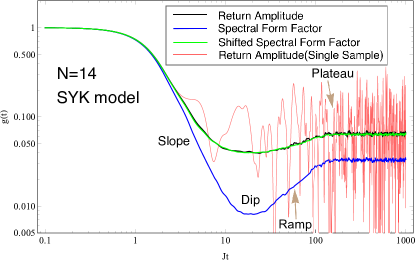
Figure 1: These are numerical plots for the $N=14$ $q=4$ SYK model. We take the disorder average for $1500$ samples except for the single sample case. We put $\beta=1.5$. The return amplitude is defined (10) and we choose the state that satisfies $S_{k}\ket{B_{\uparrow\cdots\uparrow}}=\ket{B_{\uparrow\cdots\uparrow}}$. The shifted spectral form factor is the right hand side of (7) for the SYK Hamiltonian. We normalize them so that the initial values become $1$. A single sample of $g_{p}(t)$ shows erratic oscillation around the averaged return amplitude at late time and it is not self averaging1997PhRvL..78.2280P .

Clearly, we observe the slope, the dip, the ramp and the plateau in the return amplitude in the SYK model. The early time decay is almost the same with the spectral form factor. In the large $N$ limit, $\bra{B_{s}}e^{-\beta H_{SYK}}\ket{B_{s}}=2^{-{N\over 2}}\text{Tr}(e^{-\beta H_{SYK}})+\mathcal{O}(1/N^{q-1})$ for any $\ket{B_{s}}$ Kourkoulou:2017zaj in the leading of $1/N$ expansion. The early time dependence is captured by the analytic continuation of $\beta\to\beta+it$ from the leading term in $1/N$, we expect the match between them. On the other hand, the ramp and the plateau region we do not expect that because they are non perturbative effects in $1/N$ expansionCotler:2016fpe ; Saad:2018bqo . The plot shows that they take different value at late time. The late time behavior is expected to be governed by random matrix theoryCotler:2016fpe . We also expect this to the return amplitude. To confirm this, we compare the return amplitude with the shifted spectral form factor (7) where the ensemble average $\braket{g(t;\beta)}_{\text{GUE}}$ is replaced by the SYK coupling average $\braket{g(t;\beta)}_{J}$. We also restrict the Hamiltonian to the fixed $(-1)^{F}$ charge sector in the shifted spectral form factor because only that acts on the state $\ket{B_{s}}$. The plots agree very well and these results also support the random matrix behavior in the late time in the SYK model.

3. A Deformed Hamiltonian Next we consider the following ”mass term” HamiltonianKourkoulou:2017zaj :

$$H_{M}=-{1\over 2}\sum_{k}s_{k}S_{k}=i\sum_{k}s_{k}\psi_{2k-1}\psi_{2k}.$$ (11)

This Hamiltonian is diagonalized in the $\ket{B_{s}}$ state basis. Especially, the unique ground state of this Hamiltonian is given by $\ket{B_{s}}$ with spin $\{s_{k}\}$ and energy $E_{0}^{(0)}=-N/4$. By flipping some spins from the ground state $\ket{B_{s}}$, we obtain the whole energy eigenstates. The excited state energy levels are given by

$$E_{m}^{(0)}=-{N\over 4}+m\ \text{with degeneracy}\ d_{m}=\begin{pmatrix}N/2\\ m\end{pmatrix}.$$ (12)

There are energy gaps , which is given by $E_{m+1}^{(0)}-E_{m}^{(0)}=1$, between the bands. Now we consider the Hamiltonian that contains the both of the SYK term and (11):

$$H_{def}=H_{SYK}+\mu H_{M}.$$ (13)

This Hamiltonian was originally proposed to describe the traversable wormhole after projection measurementsKourkoulou:2017zaj . We call this $H_{def}$ the deformed Hamiltonian. Here we consider the regime that $\mu$ is large and we can treat the SYK term as perturbation. This can be seen as a perturbation of the integrable system with degenerate spectrum by the chaotic Hamiltonian. . We also concentrate on the infinite temperature cases. Because $\mu$ is large, exact energy levels from $E_{i_{m}}$ with $i_{m}=d_{1}+\cdots+d_{m-1}+1$ to $E_{f_{m}}$ with $f_{m}=d_{1}+\cdots+d_{m}$ localize near $E_{m}^{(0)}$ and form band like structure. By exactly diagonalizing the Hamiltonian, we can study the return amplitude under the deformed Hamiltonian. We show the numerical results in Fig.2.

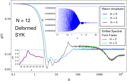
Figure 2: These are numerical plots for the $N=12$ $q=4$ deformed SYK model with $\mu=50$ and $s_{k}=1$ in (11) for all $k$. We take the average over $2000$ samples. $m$ is the number of flips of spins from the B state from the ground state of $H_{M}$. More explicitly, we choose $\ket{B_{\uparrow\uparrow\uparrow\uparrow\uparrow\uparrow}}$ for $m=0$, $\ket{B_{\downarrow\downarrow\uparrow\uparrow\uparrow\uparrow}}$ as an example of $m=2$ cases and $\ket{B_{\downarrow\downarrow\downarrow\uparrow\uparrow\uparrow}}$ for $m=3$. We also plotted the shifted spectral form factor of band $m$ where the spectral form factor is restricted on the $m$-th band is $\sum_{i,j=i_{m}}^{f_{m}}e^{-i(E_{i}-E_{j})t}$ and the shift (3) is given by $L=d_{m}$. We see the kink around the transition time from the ramp to the plateau in the $m=3$ case, which reflects GSE statisticsCotler:2016fpe .

Here we explain the results. First, the ground state of $H_{def}$ is almost given by $\ket{B_{s}}$ with $m=0$ because the gap between the ground state and the first excited states is $\mu$, which is sufficiently large and suppresses the mixing with other $\ket{B_{s}}$ states. In this case, the return amplitude does not decay and also shows oscillation at early time. The behavior of $\ket{B_{s}}$ with $m\neq 0$ are described by random matrix theory. According to the perturbation theory of quantum mechanics the first order shift of energy levels are determined by the projection of $H_{SYK}$ onto the degenerate energy levelsmessiah1999quantum . Therefore at early time the projection of $H_{SYK}$ on each degenerate energy levels determines the time evolution of $\ket{B_{s}}$. We know the dimension of the projected Hamiltonian from (12). By considering the spectral form factor restricted on the $m$-th band and its shift by $L=d_{m}$, we see the very good agreement with the return amplitude. Because the spectral form factor and the return amplitude depend on the level statistics, next we determines the symmetry class of each band. To see this, we need to know the symmetry properties of $\ket{B_{s}}$. These are eigenstates of $(-1)^{F}$. The anti unitary $\mathcal{T}$ flips the spin $\mathcal{T}S_{k}\mathcal{T}^{-1}=-S_{k}$. Therefore, we find that $\mathcal{T}\ket{B_{s}}=e^{i\theta_{s}}\ket{B_{-s}}$ where $e^{i\theta_{s}}$ is a phase factor and $\ket{B_{-s}}$ is the state that satisfies $S_{k}\ket{B_{-s}}=-s_{k}\ket{B_{-s}}$. From this, we find for the projection operator onto the flip number $m$ sector $P_{m}=\sum_{\#\text{flip}=m}\ket{B_{s}}\bra{B_{s}}$ satisfies

$$\mathcal{T}P_{m}\mathcal{T}^{-1}=P_{{N\over 2}-m}.$$ (14)

This means that $\mathcal{T}$ flips the bands.

Now we consider the symmetry class based on these properties. First we consider the $m\neq{N\over 4}$ bands. In this case, $H_{m}$ satisfies $\mathcal{T}H_{m}\mathcal{T}^{-1}=H_{{N\over 2}-m}$. Therefore, there are no constraint from the symmetry $\mathcal{T}$ and we expect GUE statistics for $H_{m}$. Next we consider $m={N\over 4}$th bands which exist in $N=0,4\ (\text{mod}\ 8)$ cases. Now $\mathcal{T}$ imposes symmetry constraint $\mathcal{T}H_{N\over 4}\mathcal{T}^{-1}=H_{N\over 4}$ and we expect GOE ensemble for $N=0\ (\text{mod}\ 8)$ and GSE ensemble for $N=4\ (\text{mod}\ 8)$ on these bands at the first order of perturbation. Except for $m={N\over 4}$th bands in $N=4\ (\text{mod}\ 8)$, we expect that degeneracies are completely removed by the SYK Hamiltonian perturbation. Because of Kramers’ degeneracies of $H_{{N\over 4}}$ that originate to the time reversal anomaly $\mathcal{T}^{2}=-1$, $m={N\over 4}$th bands in $N=4\ (\text{mod}\ 8)$ have still two degeneracies at each level at the first order perturbation. According to the second order perturbation theroymessiah1999quantum , the second order shift of degenerate spectrums is determined by $H_{{N\over 4}}^{i}=\mathcal{P}_{i}H_{SYK}\mathcal{Q}_{N\over 4}H_{SYK}\mathcal{P}_{i}$. Here $\mathcal{Q}_{{N\over 4}}=\sum_{m\neq{N\over 4}}{P_{m}\over-{N\over 4}+m}$ and $\mathcal{P}_{i}=\ket{\psi_{i,1}}\bra{\psi_{i,1}}+\ket{\psi_{i,2}}\bra{\psi_{i,2}}$ with two eigenstates of $i$-th degenerate eigenvalues. We choose the basis that satisfies $\mathcal{T}\ket{\psi_{i,1}}=\ket{\psi_{i,2}}$. From these definitions, we find that $\mathcal{T}\mathcal{P}_{i}\mathcal{T}^{-1}=\mathcal{P}_{i}$ and $\mathcal{T}\mathcal{Q}_{{N\over 4}}\mathcal{T}^{-1}=-\mathcal{Q}_{{N\over 4}}$. This means $\mathcal{T}H_{{N\over 4}}^{i}\mathcal{T}^{-1}=-H_{{N\over 4}}^{i}$. By solving this symmetry constraint in the basis with $\mathcal{T}=\begin{pmatrix}0&-1\\ 1&0\end{pmatrix}K$ , we obtain

$$H_{{N\over 4}}^{i}=\mathcal{P}_{i}H_{SYK}\mathcal{Q}_{N\over 4}H_{SYK}\mathcal{P}_{i}=\begin{pmatrix}x&a\\ a^{*}&-x\end{pmatrix},$$ (15)

with a real number $x$ and a complex number $a$. This means that in a generic Hamiltonian the off diagonal element $a$ enters and the degeneracies are removed. Therefore the degeneracy is removed at the second order of the perturbation. This difference of the order means that the return amplitude (and the spectral form factor) does not see the true degeneracy at early time. We see numerically in fig.2 that they show the first order degeneracy at the first plateau, but after that they show the second slop, dip, ramp, and plateau. The second plateau value is smaller than the first plateau value because (4) means that degeneracies give larger plateau values.

To see the level statistics further, we study the distribution of the adjacent gap ratio2015PhRvB..91h1103L ; 2007PhRvB..75o5111O ; 2016PhRvB..94n4201B ; PhysRevB.95.115150 for each $m$-th band. The adjacent gap ratio is defined as $r_{n}={E_{n+1}-E_{n}\over E_{n}-E_{n-1}}$ for an ordered spectrum $E_{n-1}<E_{n}<E_{n+1}$. The distribution of the ratio $r_{n}$ in Poisson statistics is

$$p(r)={1\over(1+r)^{2}}.$$ (16)

On the other hand, in random matrices, the distribution of the ratio $r_{n}$ becomes2013PhRvL.110h4101A

$$p(r)={1\over Z_{\beta}}{(r+r^{2})^{\beta}\over(1+r+r^{2})^{1+{3\over 2}\beta}}.$$ (17)

For GOE $\beta=1$ and $Z_{\beta}={27\over 8}$. For GUE $\beta=2$ and ${4\pi\over 81\sqrt{3}}$. For GSE $\beta=4$ and $Z_{\beta}={4\pi\over 729}$. $r\to 0$ behavior $p(r)\sim r^{\beta}$ represents the level repulsion. We study this gap ratio numerically in $N=16$ case and compare with the random matrix case. The $m={N\over 4}=4$th band shows GOE statistics and the $m=3$rd band shows GUE statistics. These result agree with our symmetry analysis above.

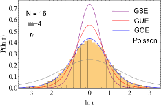
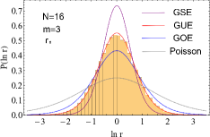
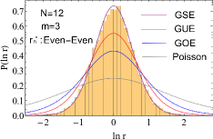
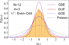
Figure 3: We plot the probability density $P(\ln r)=p(r)r$ for some examples. The solid lines are the Wigner surmise given by (16) and (17). Top: The gap ratio $r_{n}$ for $m=3$rd band and $m=4$th band in the $N=16,q=4$ deformed SYK model. We take the average over $1000$ samples. Bottom: We consider the $m=3$rd band in the $N=12,q=4$ deformed SYK model. The left is the gap ratio for even energy levels $r_{n}^{\prime}={E_{2n+2}-E_{2n}\over E_{2n}-E_{2n-2}}$. The right is the gap ratio $r_{n}^{\prime\prime}={E_{2n+2}-E_{2n+1}\over E_{2n}-E_{2n-1}}$. We take the average over $2000$ samples for both cases.

$m={N\over 4}$-th bands in $N=4\ (\text{mod}\ 8)$, the degeneracies are removed at different order of perturbation. Therefore, $E_{2n}-E_{2n-1}$ is of order $\mu^{-1}$ while $E_{2n+1}-E_{2n}$ is of order $1$. In this case we expect $E_{2n+2}-E_{2n}$ is determined by the first order perturbation and looks like GSE ensemble when $\mu$ is large. We study the gap ratio $r_{n}^{\prime}={E_{2n+2}-E_{2n}\over E_{2n}-E_{2n-2}}$ numerically and the results show GSE statistics. On the other hand, the gap ratio $r_{n}^{\prime\prime}={E_{2n+2}-E_{2n+1}\over E_{2n}-E_{2n-1}}$ is also an order one quantity because both of the numerator and the denominator are of order $\mu^{-1}$. These gap $E_{2n}-E_{2n-1}$ come from (15) that is Hermitian. Therefore we expect this ratio shows GUE statistics. We study this gap ratio $r_{n}^{\prime\prime}$ numerically and they show GUE statistics as expected.

4.Discussion The return amplitude in random matrices is exactly calculated and related to the spectral form factor. Our numerical study also shows that this relation holds in the SYK model. Initially the return amplitude decays but at late time first they grows from the dip and then saturates the plateau value. Because the random matrix behavior is expected to be universal in chaotic systems, we expect that these behaviors are true even in more generic chaotic systems like conformal field theory after a suitable average like a time average. When we deform the SYK Hamiltonian by a mass term, the return amplitude depends on the choice of initial states. If we choose the initial product states to be a ground state of the mass term, the return amplitude does not decay. This deformation prevents the initial state to be scrambled and protects from thermalization. In gravity side, we can interpret this as the disappearance of the black hole horizon and we have access to the black hole interiors. If we flip the $m$ spins from the almost ground state one, return amplitude decays and their behaviors are again explained by random matrix theory. The most interesting case is the $m={N\over 4}$ cases in $N=4$ (mod $8$) cases where we see the second dip, ramp and plateau. In early time the return amplitude behave like GSE statistics with $2$ degeneracies at each level, but at late time it realizes that the degeneracies are actually removed and finally decays to smaller values. This serves an example of the return amplitude or the spectral form factor with complicated patterns.

Acknowledgement We thank A.Maloney, S. Harrison and T.Takayanagi for useful discussions. We also thank R.Namba and D.Yoshida about discussions for numerical calculations. TN is supported by JSPS fellowships and the Simons Foundation through the It From Qubit collaboration.

Appendix A A.Explicit Realization of Majorana fermions

In this appendix we give an explicit representation of Majorana fermions. We follow the notation of Saad:2018bqo . We can realize the fermions as the tensor products of the Pauli matrices:

$$\psi_{2k-1} = {1\over\sqrt{2}}Z_{1}\cdots Z_{k-1}X_{k}I_{k+1}\cdots I_{N/2},$$

$$\psi_{2k} = {1\over\sqrt{2}}Z_{1}\cdots Z_{k-1}Y_{k}I_{k+1}\cdots I_{N/2}.$$ (18)

Here

$$X_{i}=\begin{pmatrix}0&1\\ 1&0\end{pmatrix},\ \ Y_{i}=\begin{pmatrix}0&-i\\ i&0\end{pmatrix},\ \ Z_{i}=\begin{pmatrix}1&0\\ 0&-1\end{pmatrix}$$ (19)

are the Pauli operators on $i$-th site and we omit the symbols $\otimes$ for tensor product in (18). Then, the $k$-th spin operator $S_{k}$ becomes

$$S_{k}=-2i\psi_{2k-1}\psi_{2k}=I_{1}\dots I_{k-1}Z_{k}I_{k+1}\dots I_{{N\over 2}}.$$ (20)

This confirms that $S_{k}$ is the spin operator that measure the eigenvalues of $Z_{k}$. In this basis, we can write the $\ket{B_{s}}$ state as

$$\ket{B_{s}}=\ket{s_{1}s_{2}\cdots s_{{N\over 2}}}.$$ (21)

for the state with $S_{k}\ket{B_{s}}=s_{k}\ket{B_{s}}$.

We also give the explicit form of anti unitary symmetry $\mathcal{T}$ and mod $2$ fermion number $(-1)^{F}$ in this basis. The fermion number $(-1)^{F}$ is given by

$$(-1)^{F}=\prod_{k=1}^{{N\over 2}}S_{k}=2^{N\over 2}i^{-{N\over 2}}\psi_{1}\psi_{2}\cdots\psi_{N}.$$ (22)

$\mathcal{T}$ depends on the $N$. When $N/2$ is odd case that corresponds to $N=2,6\ (\text{mod}\ 8)$ ,

$$\mathcal{T}=2^{N\over 4}K\psi_{1}\psi_{3}\cdots\psi_{N-3}\psi_{N-1},$$ (23)

where $K$ is the antiunitary operator that takes the complex conjugate. When $N/2$ is even case that corresponds to $N=0,4\ (\text{mod}\ 8)$ ,

$$\mathcal{T}=2^{N\over 4}K\psi_{2}\psi_{4}\cdots\psi_{N-2}\psi_{N}.$$ (24)

Using this explicit representation, we can show the symmetry property in Table.1. Though these realization gives a way to see the symmetry property, they are characterized by topological invariantsPhysRevB.83.075103 and independent from explicit realization.

Appendix B B. Haar integrals and the derivation of the return amplitude in Random Matrices

We derive the return amplitude in random matrix theory. The key observation is that the measure is invariant under unitary conjugation $d(U^{\dagger}HU)e^{-V(U^{\dagger}HU)}=dHe^{-V(H)}$ with $V(H)={L\over 2}\text{Tr}H^{2}$. Though we choose the potential $V(H)$ of GUE ensemble, we only need the invariance of $V(H)$ under the unitary conjugation. Then we can represent the GUE ensemble average as $\braket{f(H)}_{\text{GUE}}=\int dH\int dUe^{-{L\over 2}\text{Tr}H^{2}}f(U^{\dagger}HU)$ for any function $f(H)$ where $dU$ is the Haar measure. For the return amplitude, we get

$$\int dH\int dUe^{-V(H)}|\braket{\psi_{0}}{U^{\dagger}e^{-iHt}U}{\psi_{0}}|^{2}$$

$$= \int dH\int dUe^{-V(H)}\text{Tr}(e^{-iHt}U\Pi U^{\dagger}e^{iHt}U\Pi U^{\dagger})$$

This integral have four same unitary matrices. To evaluate this, we need the following integral:

$$\int dU_{Haar}U_{i_{1}j_{1}}U_{i_{2}j_{2}}U^{*}_{i_{1}^{\prime}j_{1}^{\prime}}U^{*}_{i_{2}^{\prime}j_{2}^{\prime}}$$

$$= {1\over L^{2}-1}(\delta_{i_{1}i_{1}^{\prime}}\delta_{i_{2}i_{2}^{\prime}}\delta_{j_{1}j_{1}^{\prime}}\delta_{j_{2}j_{2}^{\prime}}+\delta_{i_{1}i_{2}^{\prime}}\delta_{i_{2}i_{1}^{\prime}}\delta_{j_{1}j_{2}^{\prime}}\delta_{j_{2}j_{1}^{\prime}})$$

$$-{1\over L(L^{2}-1)}(\delta_{i_{1}i_{1}^{\prime}}\delta_{i_{2}i_{2}^{\prime}}\delta_{j_{1}j_{2}^{\prime}}\delta_{j_{2}j_{1}^{\prime}}+\delta_{i_{1}i_{2}^{\prime}}\delta_{i_{2}i_{1}^{\prime}}\delta_{j_{1}j_{1}^{\prime}}\delta_{j_{2}j_{2}^{\prime}}).$$

Using this integral, we obtain

$$\braket{}{\bra{\psi_{0}}e^{-iHt}\ket{\psi_{0}}}{{}^{2}}_{\text{GUE}}={1\over L(L+1)}(\braket{Z(t)Z(t)^{*}}_{\text{GUE}}+L).$$ (27)

In a similar way, we obtain

$$\braket{}{\bra{\psi_{1}}e^{-iHt}\ket{\psi_{0}}}{{}^{2}}_{\text{GUE}}={1\over L^{2}-1}\Big{(}L-{\braket{Z(t)Z(t)^{*}}_{\text{GUE}}\over L}\Big{)},$$ (28)

for orthogonal $\ket{\psi_{0}}$ and $\ket{\psi_{1}}$.

For GSE or GOE cases, the Haar integral for $U\in U(L)$ is replaced by the Haar integral for symplectic groups $S\in Sp(L/2)$ or orthogonal groups $O\in O(L)$. The Haar integral for symplectic groups are given by2006CMaPh.264..773C ; 1997PhRvB..55.1142A

$$\int dS_{Haar}S_{i_{1}j_{1}}S_{i_{2}j_{2}}S_{i_{1}^{\prime}j_{1}^{\prime}}^{*}S_{i_{2}^{\prime}j_{2}^{\prime}}^{*}$$ (29)

$$= {L-1\over L(L+1)(L-2)}(\delta_{i_{1}i_{1}^{\prime}}\delta_{i_{2}i_{2}^{\prime}}\delta_{j_{1}j_{1}^{\prime}}\delta_{j_{2}j_{2}^{\prime}}$$

$$+\delta_{i_{1}i_{2}^{\prime}}\delta_{i_{2}i_{1}^{\prime}}\delta_{j_{1}j_{2}^{\prime}}\delta_{j_{2}j_{1}^{\prime}}+C_{i_{1}i_{2}}C_{j_{1}j_{2}}C_{i_{1}^{\prime}j_{1}^{\prime}}C_{j_{1}^{\prime}j_{2}^{\prime}})$$

$$-{1\over L(L+1)(L-2)}(\delta_{i_{1}i_{1}^{\prime}}\delta_{i_{2}i_{2}^{\prime}}\delta_{j_{1}j_{2}^{\prime}}\delta_{j_{2}j_{1}^{\prime}}$$

$$+\delta_{i_{1}i_{2}^{\prime}}\delta_{i_{2}i_{1}^{\prime}}\delta_{j_{1}j_{1}^{\prime}}\delta_{j_{2}j_{2}^{\prime}}+(\delta_{i_{1}i_{1}^{\prime}}\delta_{i_{2}i_{2}^{\prime}}-\delta_{i_{1}i_{2}^{\prime}}\delta_{i_{2}i_{1}^{\prime}})C_{j_{1}j_{2}}C_{j_{1}^{\prime}j_{2}^{\prime}}$$

$$+C_{i_{1}i_{2}}C_{i_{1}^{\prime}i_{2}^{\prime}}(\delta_{j_{1}j_{1}^{\prime}}\delta_{j_{2}j_{2}^{\prime}}-\delta_{j_{1}j_{2}^{\prime}}\delta_{j_{2}j_{1}^{\prime}})),$$

where $C_{ij}$ is the antisymmetric invariant. This coupling gives the inner product between the Kramers’ pairs. Because this coupling is antisymmetric, the diagonal part $v_{i}C_{ij}v_{j}$ for $\ket{\psi_{0}}=\sum_{i}v_{i}\ket{e_{i}}$ vanishes and they can be ignored in the calculation of the return amplitude. Using this integral, we obtain

$$\braket{}{\bra{\psi_{0}}e^{-iHt}\ket{\psi_{0}}}{{}^{2}}_{\text{GSE}}={1\over L(L+1)}(\braket{Z(t)Z(t)^{*}}_{\text{GSE}}+L),$$ (30)

which is the same expression with the GUE case though the Haar integrals themselves are different.

The Haar integral for orthogonal groups are given by2006CMaPh.264..773C ; 1997PhRvB..55.1142A

$$\int dO_{Haar}O_{i_{1}j_{1}}O_{i_{2}j_{2}}O_{i_{1}^{\prime}j_{1}^{\prime}}^{*}O_{i_{2}^{\prime}j_{2}^{\prime}}^{*}$$ (31)

$$= {L+1\over L(L-1)(L+2)}(\delta_{i_{1}i_{1}^{\prime}}\delta_{i_{2}i_{2}^{\prime}}\delta_{j_{1}j_{1}^{\prime}}\delta_{j_{2}j_{2}^{\prime}}$$

$$+\delta_{i_{1}i_{2}^{\prime}}\delta_{i_{2}i_{1}^{\prime}}\delta_{j_{1}j_{2}^{\prime}}\delta_{j_{2}j_{1}^{\prime}}+C_{i_{1}i_{2}}C_{j_{1}j_{2}}C_{i_{1}^{\prime}j_{1}^{\prime}}C_{j_{1}^{\prime}j_{2}^{\prime}})$$

$$-{1\over L(L-1)(L+2)}(\delta_{i_{1}i_{1}^{\prime}}\delta_{i_{2}i_{2}^{\prime}}\delta_{j_{1}j_{2}^{\prime}}\delta_{j_{2}j_{1}^{\prime}}$$

$$+\delta_{i_{1}i_{2}^{\prime}}\delta_{i_{2}i_{1}^{\prime}}\delta_{j_{1}j_{1}^{\prime}}\delta_{j_{2}j_{2}^{\prime}}+(\delta_{i_{1}i_{1}^{\prime}}\delta_{i_{2}i_{2}^{\prime}}+\delta_{i_{1}i_{2}^{\prime}}\delta_{i_{2}i_{1}^{\prime}})C_{j_{1}j_{2}}C_{j_{1}^{\prime}j_{2}^{\prime}}$$

$$+C_{i_{1}i_{2}}C_{i_{1}^{\prime}i_{2}^{\prime}}(\delta_{j_{1}j_{1}^{\prime}}\delta_{j_{2}j_{2}^{\prime}}+\delta_{j_{1}j_{2}^{\prime}}\delta_{j_{2}j_{1}^{\prime}})),$$

where $C_{ij}$ is the symmetric coupling and we can choose a basis with $C_{ij}=\delta_{ij}$. Unlike the case of symplectic groups, the diagonal part $v_{i}C_{ij}v_{j}$ for $\ket{\psi_{0}}=\sum_{i}v_{i}\ket{e_{i}}$ does not vanish and the return amplitude depends on states.

Appendix C C. Symmetry analysis of the Deformed SYK Hamiltonian at 1st order perturbation

In this section we study the symmetry class $H_{m}$ in detail that is imposed by $\mathcal{T}$ symmetry. Because $\mathcal{T}$ relates the $m$-th band and the $({N\over 2}-m)$-th band, it is sufficient to consider the the symmetry constraint on the following submatrix:

$$H^{m,{N\over 2}-m}=\begin{pmatrix}H_{m}&S_{m}\\ S_{m}^{\dagger}&H_{{N\over 2}-m}\end{pmatrix},$$ (32)

where $H_{m}=P_{m}H_{SYK}P_{m}$ and $S_{m}=P_{m}H_{SYK}P_{{N\over 2}-m}$. Using the symmetry of the SYK Hamiltonian $(-1)^{F}H_{SYK}(-1)^{F}=H_{SYK}$, we find $P_{m}H_{SYK}P_{{N\over 2}-m}=(-1)^{{N\over 2}}P_{m}H_{SYK}P_{{N\over 2}-m}$. This means $S_{m}=0$ for $N=2,6\ (\text{mod}\ 8)$. For $N=0,2\ (\text{mod}\ 8)$ cases, $\mathcal{T}^{2}=1$. In these cases, we can choose the basis with $\mathcal{T}=\begin{pmatrix}0&\mathbb{I}_{d_{m}}\\ \mathbb{I}_{d_{m}}&0\end{pmatrix}K$ where $\mathbb{I}_{d_{m}}$ is the identity matrix of rank $d_{m}$ and $K$ is the complex conjugate operator. The invariance under this $\mathcal{T}$ imposes the condition $H_{{N\over 2}-m}^{*}=H_{m}$ and $S_{m}^{T}=S_{m}$. For $N=0\ (\text{mod}\ 8)$ this means that $H^{m,{N\over 2}-m}$ is conjugate to real symmetric matrix though $H^{m,{N\over 2}-m}$ is expressed in unusual basis in which the reality is not manifest. To see the reality manifestly, it is convenient to change the basis in the following way:

$$\begin{pmatrix}H_{m}&S_{m}\\ S_{m}^{*}&H_{m}^{*}\end{pmatrix}$$ (33)

$$\to{1\over\sqrt{2}}\begin{pmatrix}\mathbb{I}_{d_{m}}&\mathbb{I}_{d_{m}}\\ i\mathbb{I}_{d_{m}}&-i\mathbb{I}_{d_{m}}\end{pmatrix}\begin{pmatrix}H_{m}&S_{m}\\ S_{m}^{*}&H_{m}^{*}\end{pmatrix}{1\over\sqrt{2}}\begin{pmatrix}\mathbb{I}_{d_{m}}&-i\mathbb{I}_{d_{m}}\\ \mathbb{I}_{d_{m}}&i\mathbb{I}_{d_{m}}\end{pmatrix}$$

$$= \begin{pmatrix}\text{Re}H_{m}+\text{Re}S_{m}&\text{Im}H_{m}-\text{Im}S_{m}\\ -\text{Im}H_{m}-\text{Im}S_{m}&\text{Re}H_{m}-\text{Re}S_{m}\end{pmatrix}.$$

This takes the form of the real symmetric matrix under the condition $S_{m}^{T}=S_{m}$ and $H_{m}^{\dagger}=H_{m}$. Though $\mathcal{T}$ relate $H_{m}$ and $H_{{N\over 2}-m}$, it does not impose any constraint on $H_{m}$ itself. Therefore, for generic matrix $H^{m,{N\over 2}-m}$, $H_{m}$ belongs to GUE ensemble.

For $N=4,6\ (\text{mod}\ 8)$, $\mathcal{T}^{2}=-1$. In these cases, we can choose the basis with $\mathcal{T}=\begin{pmatrix}0&-\mathbb{I}_{d_{m}}\\ \mathbb{I}_{d_{m}}&0\end{pmatrix}K.$ In the same manner, we obtain $H_{m}=H_{{N\over 2}-m}^{*}$ and $S_{m}^{T}=-S_{m}$. For $N=4\ (\text{mod}\ 8)$ this means that $H^{m,{N\over 2}-m}$ is a quaternion Hermitian. We can write as $H_{m}=H+iA_{z}$ and $S_{m}=iA_{x}+A_{y}$ where $H$ is real symmetric and $A_{x},A_{y},A_{z}$ is real antisymmetric. Then, $H^{m,{N\over 2}-m}=H\otimes\mathbb{I}_{2}+\sum_{\alpha}iA_{\alpha}\otimes\sigma_{\alpha}$ gives a usual realization of quaternion Hermitian matrices. $H_{m}=H+iA_{z}$ spans generic Hermitian matrices and the ensemble is GUE. Again though $\mathcal{T}$ relate $H_{m}$ and $H_{{N\over 2}-m}$, $\mathcal{T}$ does not impose any condition on $H_{m}$ itself.

Appendix D D. Evolution Amplitude in the SYK model

In this section we consider the overlap between time evolved state $e^{-iHt}\ket{\psi_{0}}$ and states $\ket{\psi_{1}}$ that is orthogonal to $\ket{\psi_{0}}$, which we consider in random matrices in (5), in the SYK model. Especially, we consider the amplitude between $\ket{B_{s}}$ with different spins:

$$|\bra{B_{s^{\prime}}}e^{-iH_{SYK}t}\ket{B_{s}}|^{2}.$$ (34)

Here we call this the evolution amplitude. In figure.4, we compare the return amplitude and the evolution amplitude numerically in the SYK model.

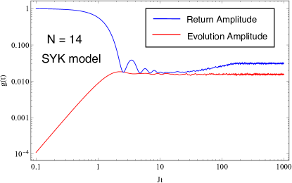
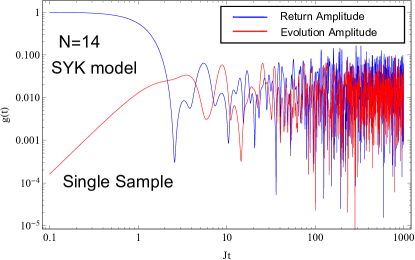
Figure 4: These are the numerical plots of the return amplitude and the evolution amplitude in the $N=14,q=4$ SYK model. As an example of the return amplitude, we consider $|\bra{B_{\uparrow\uparrow\uparrow\uparrow\uparrow\uparrow\uparrow}}e^{-iH_{SYK}t}\ket{B_{\uparrow\uparrow\uparrow\uparrow\uparrow\uparrow\uparrow}}|^{2}$, and as an example of the evolution amplitude we consider $|\bra{B_{\downarrow\downarrow\uparrow\uparrow\uparrow\uparrow\uparrow}}e^{-iH_{SYK}t}\ket{B_{\uparrow\uparrow\uparrow\uparrow\uparrow\uparrow\uparrow}}|^{2}$. Top: We take the average over $1500$ samples for both of the return amplitude and the evolution amplitude. Bottom: The return amplitude and the evolution amplitude with single sample.

After the ensemble average, they show that the plateau value in the return amplitude is clearly larger than the evolution amplitude. Even in single sample, the return amplitude looks to oscillate around the larger average value than the the evolution amplitude.

Appendix E E. Time Average of single sample in the SYK model

The spectral form factor is not self averaging1997PhRvL..78.2280P , and we need some averages to get smooth behaviors. In the SYK model, we take the ensemble average over the coupling $J_{a_{1}\cdots a_{q}}$. In this appendix, we consider the time average of the return amplitude in a single sample in the SYK model, which is another kind of average. First we consider the infinite time average , which gives the averaged plateau value, in general quantum systems without degeneracy. By decomposing the state $\ket{\psi_{0}}=\sum_{i}c_{i}\ket{E_{i}}$, we obtain

$$\lim_{T\to\infty}{1\over T}\int_{0}^{T}|\bra{\psi_{0}}e^{-iHt}\ket{\psi_{0}}|^{2}$$ (35)

$$= \lim_{T\to\infty}{1\over T}\int_{0}^{T}dt\sum_{i,j}c_{i}^{*}c_{i}c_{j}^{*}c_{j}e^{-i(E_{i}-E_{j})t}$$

$$= \sum_{i}|c_{i}|^{4}.$$

Therefore the time average is not exactly the same with the plateau value in ensemble average (3). If we take the average of (35) over states , it becomes the late time value $2/(L+1)$ in the ensemble average. In the SYK model, we consider the following time average:

$$g_{p}^{time}(t;\beta)=\int_{{1\over 2}t}^{{3\over 2}t}|\bra{B_{s}}e^{-iH_{SYK}t^{\prime}-\beta H_{SYK}}\ket{B_{s}}|^{2}dt^{\prime}.$$ (36)

Here we take the time average between ${1\over 2}t<t^{\prime}<{3\over 2}t$ around time $t$, which is taken inBalasubramanian:2016ids . We show the plots of the return amplitude and the spectral form factor with time average in figure.5. Both of the return amplitude and the spectral form factor show the slope, dip, ramp and plateau behavior. This motivate us to expect that the return amplitude in more generic quantum systems like chaotic CFTs shows these structure after the time average. We also compare the shifted spectral form factor (35) where the ensemble average of the spectral form factor is replaced by the time average. As we pointed out, their late time value is not exactly the same, but the behavior shows good agreement on each time.

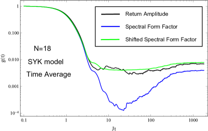
Figure 5: This is the plot of the return amplitude in the $N=18,q=4$ SYK model with the time average. We choose $\ket{B_{\uparrow\uparrow\uparrow\uparrow\uparrow\uparrow\uparrow\uparrow\uparrow}}$ as the initial state. We can see the slope, dip, ramp and plateau even in the time average cases. As we mentioned, the plateau value of the time averaged return amplitude have a small deviation from the shifted spectral form factor.