The extended Baryon Oscillation Spectroscopic Survey: measuring the cross-correlation between the MgII flux transmission field and quasars and galaxies at $z=0.59$

Abstract

We present the first attempt at measuring the baryonic acoustic oscillations (BAO) in the large scale cross-correlation between the magnesium-II doublet (MgII) flux transmission field and the position of quasar and galaxy tracers. The MgII flux transmission continuous field at $0.3<z<1.6$ is measured from 500589 quasar spectra obtained in the Baryonic Oscillation Spectroscopic Survey (BOSS) and the extended BOSS (eBOSS). The position of 246697 quasar tracers and 1346776 galaxy tracers are extracted from the Sloan Digital Sky Survey (SDSS) I, II, BOSS and eBOSS catalogs. In addition to measuring the cosmological BAO scale and the biased matter density correlation, this study allows tests and improvements to cosmological Lyman-$\alpha$ analyses. A feature consistent with that of the BAO is detected at a significance of $\Delta\chi^{2}=7.25$. The measured MgII linear transmission bias parameters are $b_{\mathrm{MgII(2796)}}(z=0.59)=(-6.82\pm 0.54)\,\times 10^{-4}$ and $b_{\mathrm{MgII(2804)}}(z=0.59)=(-5.55\pm 0.46)\,\times 10^{-4}$, and the MgI bias is $b_{\mathrm{MgI(2853)}}(z=0.59)=(-1.48\pm 0.24)\,\times 10^{-4}$. Their redshift evolution is characterized by the power-law index: $\gamma_{\mathrm{Mg}}=3.36\pm 0.46$. These measurements open a new window towards using BAO from flux transmission at $z<1$ in the final eBOSS sample and in the upcoming sample from the Dark Energy Spectroscopic Instrument.

,

1. Introduction

The intergalactic medium (IGM) gas traces the underlying distribution of baryonic matter and dark matter. In spectra of background quasars, the fluctuations in density of the IGM are observed as a continuous field of absorption with respect to the unabsorbed emission of the object (Gunn & Peterson, 1965; Lynds, 1971). Different atomic transitions are used to trace these density fluctuations. The Lyman-$\alpha$ (Ly$\alpha$) transition from the first orbital to the second orbital of the hydrogen atom produces the strongest signal. The continuum of absorption from Ly$\alpha$, tracing the overall fluctuations of matter density is called the Ly$\alpha$ forest. For redshift $z>2$, it can be observed from ground-based instruments. To probe lower redshifts with this technique, because of atmospheric UV cut-off, it is necessary either to observe quasars from space-based instruments (e.g., Bahcall et al., 1993; Khaire et al., 2018) or to use weaker metal transitions, as suggested by Pieri (2014), such as singly-ionized magnesium (magnesium-II; e.g., Pérez-Ràfols et al., 2015) or triply-ionized carbon (carbon-IV; e.g., Blomqvist et al., 2018; Gontcho A Gontcho et al., 2018).

Tracers of the total matter density field are used in cosmology to measure the biased 3D correlation of matter, host of the baryon acoustic oscillations (BAO), first detected in galaxies (Eisenstein et al., 2005; Cole et al., 2005). This latter feature is used as a probe of the cosmic expansion history. At lower redshift ($z<2$) the BAO scale has been measured using galaxies (Percival et al., 2007, 2010; Blake et al., 2011; Beutler et al., 2011; Chuang & Wang, 2012; Padmanabhan et al., 2012; Mehta et al., 2012; Xu et al., 2013; Anderson et al., 2012, 2014b, 2014a; Ross et al., 2015; Alam et al., 2017; Bautista et al., 2018) and quasars (Ata et al., 2018). At larger redshift ($z>2$) the number density of visible objects declines drastically and thus the measurement has been made through the Ly$\alpha$ forests auto-correlation (Busca et al., 2013; Slosar et al., 2013; Kirkby et al., 2013; Delubac et al., 2015; Bautista et al., 2017) and through the Ly$\alpha$-quasar cross-correlation (Font-Ribera et al., 2014; du Mas des Bourboux et al., 2017).

The two methods of extracting the BAO scale differ in technique and possible sources of systematic errors. One method uses the position of galaxies or quasars as discrete tracers of the denser regions of the matter density field, the other uses the IGM absorption as a continuous tracer of the entire matter density field along the line-of-sight of a quasar. BAO measurements via these two methods at the same redshift would enable different systematic tests. As yet this comparison has not been accomplished, although some steps in this direction have been investigated. Laurent et al. (2016) measured the 3D auto-correlation of quasars at $z>2$, but do not report a measurement of BAO. Blomqvist et al. (2018) measured the 3D cross-correlation between the carbon-IV (CIV) absorption in quasar spectra and the quasar distribution with a large fraction of data at $z<2$; however, they lack a detection of the BAO scale of comparable precision to discrete tracers. Pérez-Ràfols et al. (2015) measured the small scale cross-correlation between magnesium-II absorbers (MgII) and galaxies at $z\approx 0.5$, but did not investigate separations larger than $10\,\mathrm{Mpc}$.

This study uses the MgII absorption observed in background quasar spectra as a continuous tracer of the matter density field to measure the 3D cross-correlation with galaxies and quasars. Singly ionized magnesium, MgII, traces metal-enriched, photo-ionized gas in the circumgalactic medium of galaxies. In the range of optical spectroscopy with sufficient UV strength and isolation from strong atmospheric emission, $3600<\lambda<7235\,\text{\AA{}}$, MgII covers a large redshift range: $0.29<z<1.59$. In this interval, multiple BAO measurements have been reported from galaxies (e.g., Alam et al., 2017), allowing for possible comparisons between discrete and continuous samples of the matter density field. Our analysis treats the MgII absorption as a continuous field as in Zhu et al. (2014) and in Pérez-Ràfols et al. (2015), instead of as a catalog of discrete tracers as done by Gauthier et al. (2009) and Lundgren et al. (2009). Treating MgII as a discrete tracer yields a MgII bias of order unity. Blomqvist et al. (2018) studied CIV as an absorption continuous field; they measured $b_{\mathrm{CIV}}(z=2)\approx-1.4\times 10^{-2}$ for the effective bias of the CIV doublet transition.

The benefits of treating MgII as continuous absorption are: 1) there is no need to identify individual absorbers, 2) there is no confusion with other doublets (e.g., CIV, SiIV) when cross-correlating with quasars or galaxies, and 3) there is no need to build a catalog of randoms and masks of the selected spectroscopic targets. However, the main drawback of this approach is to mix signal from a small number of pixels (spectral data point of a given wavelength width) with strong MgII absorption, with numerous pixels without significant absorption. This technique has the consequence of producing a low bias compared to discrete MgII bias.

This approach of treating MgII as a continuous tracer is analogous to how Ly$\alpha$ is treated in BAO studies (e.g., Bautista et al., 2017), thus allowing us to test the Ly$\alpha$ analyses methodology in different regimes.

• The Ly$\alpha$ transition is a singlet, while the MgII transition is a doublet composed of MgII(2796): $\lambda_{\mathrm{R.F.}}=2796.35\,\text{\AA{}}$ and of MgII(2804): $\lambda_{\mathrm{R.F.}}=2803.53\,\text{\AA{}}$. The measured 3D cross-correlation with galaxies or with quasars is therefore the superposition of two correlations separated by $7\,\text{\AA{}}$ ($\sim 9\,h^{-1}~{}\mathrm{Mpc}{}$ at $z=0.59$) and of slightly different bias. This scenario allows a test of the Ly$\alpha$ analyses in the regime where multiple extra correlations are superimposed.

• The MgII bias is orders of magnitude lower than that of Ly$\alpha$. Systematic errors linked to, for example, residuals of the sky subtraction or flux calibration, would be more important in a correlation involving MgII than Ly$\alpha$.

• The MgII absorption is visible down to $z=0.29$, thus enabling a cross-correlation of the absorption field with both quasars and galaxies. The Ly$\alpha$ field is not visible at $z<2$ in optical spectra, thus it can only be cross-correlated with quasars in current spectroscopic samples. MgII allows a comparison of the two tracers (galaxy and quasars) and a test of possible systematic errors associated with the different discrete tracers.

• The shape and variation of shape of the different MgII forests (sec. 2.2) differs from the shape of the Ly$\alpha$ forest. This trait allows a search for a source of systematic errors arising from the quasar continuum.

• As discussed in Bautista et al. (2017), one possible source of systematic errors in the Ly$\alpha$ forest auto-correlation is the unavoidable presence of all auto-correlations of the different metal-absorption features. An independent measure of the bias of the MgII doublet would allow a better estimate of this systematic error.

We report measurements of the baryonic acoustic oscillations in the 3D cross-correlation of MgII and galaxies or quasars. In section 2, we present the catalogs of galaxies and quasars as tracers of matter density fluctuations and the catalog of quasars as background to the MgII absorption. We also detail the analysis to measure the absorption fluctuations against estimates of the unabsorbed quasar continuum. In section 3, we study the different metal transitions that contaminate our measurement using the auto-correlation of pixels from the same background quasar. Section 4 presents how we measure the cross-correlation between MgII absorptions and quasars or galaxies and we report the measured correlation functions. In section 5, we describe the fit to the measured cross-correlations and the resulting measurement of MgII bias and BAO parameters. In section 6, we finish with a summary and conclusion.

2. Data samples and reduction

The study presented here uses data from the Sloan Digital Sky Survey (SDSS: York et al., 2000). Most of the tracer quasars, tracer galaxies, and the entirety of the background quasars were gathered during SDSS-III by the Baryon Oscillation Spectroscopic Survey (BOSS: Eisenstein et al., 2011; Dawson et al., 2013), and during SDSS-IV by the extended BOSS (eBOSS: Dawson et al., 2016; Blanton et al., 2017). A small fraction of tracers were observed during SDSS-I and II. These data are publicly available in the fourteenth data release (DR14: Abolfathi et al., 2018), and in the seventh data release (DR7: Abazajian et al., 2009). All of these data were acquired with the $2.5$ m Sloan Foundation telescope (Gunn et al., 2006) at the Apache Point Observatory.

The catalog of quasar tracers is taken from the DR14 quasar catalog (DR14Q), presented in Pâris et al. (2018). The catalog of galaxy tracers is a combination of three different catalogs: Luminous Red Galaxies (LRG) from eBOSS (Bautista et al., 2018), LRGs from BOSS (Reid et al., 2016) and galaxies from SDSS DR7, mainly from the main sample (Blanton et al., 2005). All quasar spectra used to measure the MgII absorption field were obtained using the BOSS spectrographs (Smee et al., 2013), which have a spectral resolution of $\approx 2000$.

2.1. Catalog of quasars and galaxies

Figure 1.— Distribution of the 246697 quasars and 1346776 galaxies used as discrete tracers of the matter density fluctuations. These objects have redshifts $0.21<z<1.76$. The quasars are drawn from SDSS DR14Q and the galaxies from SDSS DR7, BOSS DR12, and eBOSS DR14.

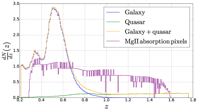
Figure 2.— Normalized redshift distribution of pixels tracing MgII absorption (delta), quasars and galaxies used as tracers of the matter density fluctuations. The flux absorption pixels are given by the $\mathrm{MgII(2796)}$ transition: $z=\lambda_{i}/\lambda_{\mathrm{MgII(2796)}}-1$. The redshift range of discrete tracers is fixed to lie within $0.21<z<1.76$. The redshift range of the pixels is bound by $0.29<z<1.59$. The pixel distribution has an apparent discretization produced by sky emission lines and Milky Way absorption features that are masked in this analysis. The quasar catalog and pixels are taken from SDSS DR14Q. The galaxy catalog is taken from SDSS DR7, BOSS DR12 and eBOSS DR14.

In this study, we use discrete tracers with redshift $0.21<z<1.76$; this range is determined by the spectrograph efficiency, the sky emission, the wavelength of the $\mathrm{MgII(2796)}$ absorption and the scale of BAO (sec. 2.2, sec. 4.1). Throughout, we refer to these discrete tracers as simply “objects”.

In the redshift range relevant to our study, $0.21<z<1.76$, we have 246697 quasar tracers observed in SDSS-I, II, BOSS and eBOSS. From the DR14Q catalog, we obtain the sample of quasars which are the background to the different forests from which we measure the $\mathrm{MgII(2796)}$ absorption. We keep only objects observed in BOSS (Ross et al., 2012) and eBOSS (Myers et al., 2015) because the small fraction of DR7 data not re-observed in BOSS or eBOSS have been observed with a different spectrograph and have been processed with a different pipeline. We remove all objects with a broad absorption line (BAL) feature following the automated index BI_CIV in DR14Q. Removing these peculiar objects improves the significance of our measurement. We also remove the few quasars with $z>5$ since their number density is low and thus do not contribute significantly to our measurement. This final sample of background quasars is composed of 500589 objects with redshift $0.35<z<5$.

In the redshift range relevant to our study, $0.21<z<1.76$, we have 94472 eBOSS galaxies, 1197675 BOSS galaxies and 170151 SDSS DR7 galaxies. We combine these three catalogs since they have similar bias that follows the same empirical law (left panel of figure 7, described in sec. 5.1). We remove possible duplicates across catalogs by excluding galaxies within one arc-second of another galaxy. In a similar manner, we remove duplicates between the galaxy and quasar catalogs. The final galaxy tracer catalog is composed of 1346776 objects. The celestial footprint of the galaxy and quasar tracers is given in figure 1 and their redshift distribution, as well as the MgII absorption pixels, in figure 2.

2.2. Measurement of the flux transmission field

To compute the fluctuation of flux transmission in the 500589 background quasars of redshift $0.35<z<5$, we use the Python “Package for IGM Cosmological-Correlations Analyses” (picca). This package has been used to perform an analysis of BAO in the cross-correlation of BOSS Ly$\alpha$ forests and quasars (du Mas des Bourboux et al., 2017, hereafter “dMdB2017”) and in the cross-correlation of eBOSS CIV forests and quasars (Blomqvist et al., 2018, hereafter “Blomqvist2018”). Using a catalog of quasars such as that described in section 2.1, picca processes all of the spectra, including those with multiple epochs. The main purpose of the package is to compute the mean unabsorbed continuum of each quasar and to compute the flux decrement at each pixel for each forest. The same package also computes and fits the cross-correlation functions.

The spectra are processed using the final eBOSS pipeline v5_11_0 (Bolton et al., 2012; Albareti et al., 2017) that will be used for DR16. For each background DR14Q quasar, we co-add all the available good observations from the spPlate files.

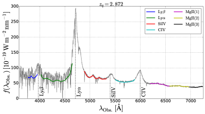
Figure 3.— Example of two eBOSS quasars and the independent fit of all the forests of table 1. The different colored lines indicate the quantity $\overline{F}(\lambda)C_{q}(\lambda_{\mathrm{R.F.}})$, from equation 1. Left: the quasar has a redshift $z=2.872$ and is identified by $(\mathrm{Plate},\mathrm{MJD},\mathrm{Fiber})=(5138,55830,20)$. Right: the quasar has a redshift $z=1.245$ and is identified by $(\mathrm{Plate},\mathrm{MJD},\mathrm{Fiber})=(4300,55528,224)$. The gray dashed lines are the location of the Ly$\beta$, Ly$\alpha$, SiIV, CIV, CIII] and MgII quasar emission lines.

To reduce the variance of the spectral pixels, we keep only data with observed wavelength $\lambda\in[3600,7235]\,\text{\AA{}}$. The lower bound of this range is set by the low system throughput at shorter wavelengths. The upper bound is given by the increasing number of sky emission lines. We mask small intervals of the observed wavelength range corresponding to remaining sky emission lines and Milky Way absorption CaII H&K (DR14 line mask in picca).

As observed in multiple analyses (e.g., Busca et al., 2013) the eBOSS pipeline produces flux calibration errors from uncertainties in the features of spectral standard F-star templates and sky emission. This miscalibration results in errors at the $3\%$ level on small wavelength scales. Furthermore, the pipeline estimates of the pixel variance are biased by up to $30\%$. In this study, we use the flux on the red side of the MgII emission line, $\lambda_{\mathrm{R.F.}}\in[2900,3120]\,\text{\AA{}}$, to correct for these two aspects. This interval of the background quasar spectra is largely free from IGM absorption, including MgII. To compute the necessary corrections, we analyze data from the longer wavelengths in the same manner as described below for the different forests. The correction of the flux calibration has no systematic impact on our final measurement, and the correction of the variance estimates only improves the significance of the final result.

To limit the loaded memory and increase the speed of the extraction of flux transmission measurements, we combine three pipeline pixels into one analysis pixel. The resulting width in observed wavelength is $\Delta\log_{10}{\lambda}=3\times 10^{-4}$. In the following, we refer to this combined pixel as simply a pixel. We also divide the spectra into $15$ different intervals in rest-frame wavelength. We refer to each distinct interval as a forest. Table 1 lists the definition of each forest, while figure 3 presents two examples of these forests in quasar spectra. Figure 3 and table 1 show that the MgII(3) and MgII(4) forests have a contribution from the CIII](1909) emission line. Variations on the strength of this line will produce correlation between pixels of the same background quasar and an increase of variance in our measurement. However, because the emission is uncorrelated from quasar to quasar, it will not bias our measurement of the MgII-tracer cross-correlation. We limit this effect in other forests by excluding the pixels in the Ly$\beta$, Ly$\alpha$, SiIV and CIV emission lines. In doing so, we maintain the same definition of forests as previous studies (e.g., dMdB2017, Blomqvist2018).

Name	$\lambda_{\mathrm{R.F.,\,\min}}$	$\lambda_{\mathrm{R.F.,\,\max}}$	$z_{\mathrm{q,\,\min}}$	$z_{\mathrm{q,\,\max}}$	$N_{q}$	$N_{pix}$
	$[\text{\AA}]$	$[\text{\AA}]$				$[10^{6}]$
$\mathrm{Ly\beta}$	$974$	$1020$	$2.65$	$5.00$	$\num{64041}$	$4$
$\mathrm{Ly\alpha}$	$1040$	$1200$	$2.10$	$5.00$	$\num{187771}$	$31$
$\mathrm{SiIV}$	$1260$	$1375$	$1.71$	$4.55$	$\num{246915}$	$30$
$\mathrm{CIV}$	$1420$	$1520$	$1.45$	$3.92$	$\num{285954}$	$27$
$\mathrm{MgII(1)}$	$1600$	$1700$	$1.19$	$3.37$	$\num{317005}$	$27$
$\mathrm{MgII(2)}$	$1700$	$1800$	$1.07$	$3.11$	$\num{319706}$	$25$
$\mathrm{MgII(3)}$	$1800$	$1900$	$0.96$	$2.88$	$\num{315419}$	$23$
$\mathrm{MgII(4)}$	$1900$	$2000$	$0.86$	$2.68$	$\num{308755}$	$22$
$\mathrm{MgII(5)}$	$2000$	$2100$	$0.77$	$2.50$	$\num{292241}$	$19$
$\mathrm{MgII(6)}$	$2100$	$2200$	$0.69$	$2.33$	$\num{263193}$	$17$
$\mathrm{MgII(7)}$	$2200$	$2300$	$0.62$	$2.18$	$\num{228279}$	$14$
$\mathrm{MgII(8)}$	$2300$	$2400$	$0.55$	$2.04$	$\num{209410}$	$12$
$\mathrm{MgII(9)}$	$2400$	$2500$	$0.49$	$1.91$	$\num{185835}$	$11$
$\mathrm{MgII(10)}$	$2500$	$2600$	$0.43$	$1.80$	$\num{163280}$	$9$
$\mathrm{MgII(11)}$	$2600$	$2760$	$0.35$	$1.69$	$\num{165784}$	$13$

Table 1 Definition of the $15$ different forests used in this study. The columns list 1) the name of the forest, 2,3) the rest-frame wavelength range, 4,5) the background quasar redshift range that have at least $50$ pixels in the given forest, with observed wavelength in $[3600,7235]\,\text{\AA{}}$, and 6,7) the total number of background quasars and pixels that contribute to each region.

In the following, we present the definition and the computation of the fluctuation of flux transmission for each forest. In this analysis, each forest is treated independently. This method is similar to the one presented in studies of Ly$\alpha$ absorption from Ly$\alpha$ forests (Bautista et al., 2017, dMdB2017) and is the same as the method presented in studies of CIV absorption in the Ly$\alpha$, SiIV and CIV forests (Blomqvist2018).

For each background quasar $q$, and for each forest, defined in table 1, the transmitted flux at each pixel delta$(q,\lambda)$, is:

$$\delta_{q}(\lambda)=\frac{f_{q}(\lambda)}{\overline{F}(\lambda)C_{q}(\lambda_{\mathrm{R.F.}})}-1,$$ (1)

where $\lambda$ is the observed wavelength, and $f_{q}(\lambda)$ is the observed flux.

In dMdB2017, $\overline{F}(\lambda)$ was the mean transmitted flux fraction between $0$ and $1$. In this study, as in Blomqvist2018, $\overline{F}(\lambda)$ is the stack of the flux in observed wavelength, normalized so that its average over the full wavelength range is one. $C_{q}(\lambda_{\mathrm{R.F.}})$ is the continuum of the given forest for the given quasar. The product $\overline{F}C_{q}$ is thus the mean expected flux for this quasar. To account for variability from background quasar to background quasar we define the continuum by:

$$C_{q}(\lambda_{\mathrm{R.F.}})=\overline{C}(\lambda_{\mathrm{R.F.}})\left[a_{q,0}+a_{q,1}\log{\lambda_{\mathrm{R.F.}}}\right],$$ (2)

where $(a_{0},a_{1})_{q}$ is a set of two free parameters fitted to the observed flux. The mean continuum $\overline{C}(\lambda_{\mathrm{R.F.}})$ is the stack of the flux over all rest-frame wavelengths and is normalized so that its mean over each forest is equal to one. For the Ly$\alpha$ and Ly$\beta$ forests, we correct the shape of the continuum for the absorption of Damped Ly$\alpha$ Absorbers (DLAs) using the automatic DR14 catalog (Noterdaeme et al., 2009, 2012). We mask pixels with more than $20\%$ absorption of the flux by the DLA. Figure 3 presents the quantity $\overline{F}(\lambda)C_{q}(\lambda_{\mathrm{R.F.}})$ for each of the $15$ forests, fitted onto two background quasars.

The weight of each delta is given by:

$$1/w_{q}(\lambda)=\eta(\lambda)\sigma^{2}_{\mathrm{noise},q}(\lambda)+\sigma^{2}_{\mathrm{LSS}}(\lambda)+\epsilon(\lambda)/\sigma^{2}_{\mathrm{noise},q}(\lambda),$$ (3)

where $\sigma_{\mathrm{noise},q}=\sigma_{\mathrm{pip},q}(\lambda)/|\overline{F}(\lambda)C_{q}(\lambda_{\mathrm{R.F.}})|$. The first term is the contribution of the measurement error; it is taken from the pipeline error corrected by the factor $\eta(\lambda)$. The second term is the Large Scale Structure (LSS) variance of each forest at a given observed wavelength. It also acts as a cap for high signal-to-noise ratio spectra. Finally the third term is the observed effect at large signal-to-noise ratio linked to the mismatch between the modeled continuum and the true observed spectra. Each of these terms are different for each forest of table 1: the resulting $\eta$ is very similar across forests, however $\epsilon$ and $\sigma^{2}_{\mathrm{LSS}}$ differ by orders of magnitude. As expected, the variance due to large scale structure is high in the Ly$\alpha$ and in the Ly$\beta$ forest, of order $10^{-1}$, whereas in other forests it is less than $5\times 10^{-3}$. This behavior can be observed in the left panel of figure 3, where the variance of the pixels bluewards of the Ly$\alpha$ emission line ($\lambda_{\mathrm{R.F.}}=1215.67$ Å, $\lambda=4707$ Å) is larger than the one of pixels redwards of the emission line. Although MgII absorption is expected to be present in all forests, its effective contribution to the observed pixel strength varies considerably across them.

As explained in dMdB2017 and Bautista et al. (2017), the fit of the continuum of equation 2 produces a distortion of the delta field. As it was done in these previous studies, we decided to make this distortion exact by redefining our field by:

$$\delta_{q}(\lambda)\rightarrow\delta_{q}(\lambda)-\overline{\delta_{q}}-\left(\Lambda-\overline{\Lambda_{q}}\right)\frac{\overline{\left(\Lambda-\overline{\Lambda_{q}}\right)\delta_{q}}}{\overline{\left(\Lambda-\overline{\Lambda_{q}}\right)^{2}}},$$ (4)

where $\Lambda\equiv\log{\lambda}$, and the mean is taken over all pixels of a given background quasar forest $q$. The second step of making this bias exact is to subtract the mean delta in bins of observed wavelength:

$$\delta_{q}(\lambda)\rightarrow\delta_{q}(\lambda)-\overline{\delta}(\lambda).$$ (5)

The quantities $\overline{F}$, $\overline{C}$, $\eta$, $\sigma^{2}_{\mathrm{LSS}}$, and $\epsilon$ are computed for each of the $15$ forests via an iterated process until they all converge. This computation results in a total of $284\times 10^{6}$ measurements of the flux-transmission, tracing the fluctuations of MgII density in the IGM. The statistics per forest are given in table 1. Figure 2 presents the redshift distribution of these pixels assuming all the absorption is from MgII. This distribution has an apparent discretization produced by sky emission lines and Milky Way absorption features which are masked in this analysis.

3. The one-dimensional pixel auto-correlation

This section presents the measurement of the auto-correlation of pixels from the same forest and from the same background quasar. This correlation allows us to identify all the different metal absorptions present in our measurement of the MgII - quasar and MgII - galaxy cross-correlations.

The normalized one-dimensional pixel auto-correlation is given by the mean of the product of two deltas:

$$\xi^{\mathrm{1D}}_{\mathrm{Norm},\,A}=\frac{\sum\limits_{\lambda_{i}/\lambda_{j}\in A}w_{i}w_{j}\frac{\delta_{i}\delta_{j}}{\sigma(\lambda_{i})\sigma(\lambda_{j})}}{\sum\limits_{\lambda_{i}/\lambda_{j}\in A}w_{i}w_{j}}.$$ (6)

In this equation $(i,j)$ is a pair of pixels from the same forest, of transmitted flux fractions $\delta_{i}$ and $\delta_{j}$, of weights $w_{i}$ and $w_{j}$, and of observed wavelengths $\lambda_{i}$ and $\lambda_{j}$ (eqns. 1 and 3). $\sigma^{2}(\lambda_{i})=\langle\delta^{2}(\lambda_{i})\rangle$ is the measured variance of the delta at a given observed wavelength. $A=(\lambda_{1}/\lambda_{2})_{A}$ is one bin of the correlation. The ratio $\lambda_{1}/\lambda_{2}$ lies in the interval $[1,\lambda_{\mathrm{R.F.,\,\max}}/\lambda_{\mathrm{R.F.,\,\min}}]$, different for each forest. As it is defined, the function gives the physical correlation within $[-1,1]$ for all pairs of pixels at a given separation of wavelength. This function is exactly $1$ ($100\%$ correlated) for $\lambda_{1}=\lambda_{2}$.

This correlation function is different for each forest defined in table 1. The auto-correlations are presented in dMdB2017 for the Ly$\alpha$ forest, and in Blomqvist2018 for the SiIV and CIV forests. Figure 4 presents the auto-correlation only for the MgII(5) forest; other MgII(i) 1D auto-correlations are similar. Several peaks corresponding to flux absorbed by correlated metals are identified in this figure.

Figure 4.— Normalized 1D auto-correlation of pixels from the same background quasar in the MgII(5) forest. The two blue dashed lines represent the $\mathrm{MgII(2796)}$ - metal correlation relevant to our study. The other black dashed lines show metal 1 - metal 2 correlations irrelevant to this study. This correlation was computed using SDSS spCFrame instead of spPlate using a pixel size of $\Delta\log_{10}{\lambda}=1\times 10^{-4}$.

To know which metal transitions will impact our cross-correlation study, we must incorporate the maximal wavelength separation relevant to the scales explored in the cosmology analysis. To study the BAO scale, we measure the MgII - object cross-correlation up to $\pm 200\,h^{-1}~{}\mathrm{Mpc}$ along the line-of-sight (sec. 4.1). At $\lambda=4600\,\text{\AA}$, this distance translates into a wavelength ratio of $\lambda_{1}/\lambda_{2}=1.06$, with respect to $\mathrm{MgII(2796)}$. We use the measured stack of absorption in quasar spectra from York et al. (2006), Pieri et al. (2014) and Mas-Ribas et al. (2017) to list all the metal transitions such that $\lambda_{1}/\lambda_{\mathrm{MgII(2796)}}\in[1/1.06,1.06]$. Only three metal transitions satisfy this condition: MgII(2796), our reference, MgII(2804), the other doublet member, and MgI(2853), absorption from neutral magnesium. Information on these two transitions is provided in table 2. The presence of these three metals in our quasar spectra data set is confirmed by the two correlation peaks marked by dashed blue lines in figure 4: $\mathrm{MgII(2796)\,/\,MgII(2804)}$ and $\mathrm{MgII(2796)\,/\,MgI(2853)}$.

$\mathrm{Transition}$	$\lambda_{\mathrm{R.F.}}$	$\lambda_{1}/\lambda_{\mathrm{MgII(2796)}}$	$r_{\parallel}$
	$[\text{\AA}]$		$[h^{-1}~{}\mathrm{Mpc}]$
MgII(2796)	$2796.35$	$1$	$0$
MgII(2804)	$2803.53$	$1.0026$	$+9$
MgI(2853)	$2852.96$	$1.0202$	$+68$

Table 2 List of the metal transitions present in the MgII - object cross-correlation. The columns are 1) the name of the transition, 2) the rest-frame wavelength, 3) the ratio $\lambda_{1}/\lambda_{\mathrm{MgII(2796)}}$, and 4) the expected shift in $h^{-1}~{}\mathrm{Mpc}$, according to the $\Lambda$CDM cosmology, of the cross-correlation at $\lambda=4446\,\text{\AA}$ ($z=0.59$ for MgII(2796)).

Figure 4 displays other metal correlations marked by black dashed lines involving different FeII transitions, but not involving MgII(2796). These metal transitions produce peaks in our correlation that are too far from our separation of $\pm 200\,h^{-1}~{}\mathrm{Mpc}$ along the line-of-sight. Thus, they are irrelevant to our cross-correlation study. Contrary to pixel auto-correlations, a pixel-object cross-correlation can only mis-interpret the redshift of the pixel because the redshift of the object is measured with low catastrophic failure rate. The consequence is that when using MgII(2796) as the reference redshift, absorption due to MgII(2796) will produce a peak in the cross-correlation at $r_{\parallel}{}=0\,h^{-1}~{}\mathrm{Mpc}{}$, while absorption due to MgI(2853) will produce a peak in the cross-correlation at $r_{\parallel}{}\sim+68\,h^{-1}~{}\mathrm{Mpc}{}$ (table 2) given the effective redshift of our sample. For FeII(2600), the peak is at $-248\,h^{-1}~{}\mathrm{Mpc}{}$; the other FeII transitions are even further remote from our $\pm 200\,h^{-1}~{}\mathrm{Mpc}$ range.

4. The MgII - quasar and MgII - galaxy cross-correlation

This section presents the measurement of the MgII - quasar and MgII - galaxy cross-correlation in each forest, along with their associated covariance matrices and the model to account for distortions introduced by continuum fitting.

4.1. The correlation function

The biased cosmological cross-correlation is calculated independently for each set of forest-object pairs. We follow the same techniques as in Font-Ribera et al. (2012, 2013) and dMdB2017. The cross-correlation is given by the weighted mean of delta from one forest at a given separation of an object:

$$\xi^{q\,f}_{A}=\frac{\sum\limits_{(i,k)\in A}w_{i}\,\delta_{i}}{\sum\limits_{(i,k)\in A}w_{i}}.$$ (7)

In this equation $i$ is a pixel of one of the forests (table 1) of transmitted flux fraction $\delta_{i}$ and weight $w_{i}$. The sum runs over all possible pixel $(i)$ - object $(k)$ pairs falling inside the bin $A=\left(r_{\parallel},r_{\perp}\right)_{A}$. We reject pairs involving a quasar and a pixel from its own forest, since the correlation vanishes for these pairs due to the fit of the continuum of equation 2.

The distance along the line-of-sight, or parallel distance, $r_{\parallel}$, and the distance across the line-of-sight, or perpendicular distance, $r_{\perp}$, are given by:

$$\begin{array}[]{ll}r_{\parallel}=\left[D_{M}(z_{i})-D_{M}(z_{k})\right]\cos\left(\frac{\Delta\theta}{2}\right),\\ r_{\perp}=\left[D_{M}(z_{i})+D_{M}(z_{k})\right]\sin\left(\frac{\Delta\theta}{2}\right).\end{array}$$ (8)

In this study we will also use the quantity $\vec{r}=(r,\mu)$, where $r^{2}=r_{\parallel}^{2}+r_{\perp}^{2}$ and $\mu=r_{\parallel}/r$. In the two relationships defined in equation 8, $\Delta\theta$ is the angle between the pixel in the forest and the object on the celestial sphere, $z_{k}$ is the redshift of the object, and $z_{i}=\lambda_{i}/\lambda_{\mathrm{MgII(2796)}}-1$ is the redshift of the pixel assuming the absorption is due to the metal transition $\mathrm{MgII(2796)}$. Finally, the comoving angular distance, $D_{M}(z)$, is computed assuming the fiducial flat-$\Lambda$CDM cosmology of Planck Collaboration et al. (2016) (TT+lowP combination):

$$\begin{array}[]{ll}\Omega_{\rm c}h^{2}=0.1197,\,\Omega_{\rm b}h^{2}=0.02222,\,\Omega_{\nu}h^{2}=0.0006,\\ h=0.6731,\,N_{\nu}=3,\,\sigma_{8}=0.830,\,n_{s}=0.9655.\end{array}$$ (9)

This cosmology has a density of matter $\Omega_{m}=0.315$, a density of dark energy $\Omega_{\Lambda}=1-\Omega_{m}=0.685$, a growth rate of structure $f(z=0.59)=0.79$, and $\sigma_{8}(z=0.59)=0.61$.

Given the fiducial cosmology, we compute the sound horizon at the drag epoch using CAMB (Lewis et al., 2000): $r_{d}=99.17\,h^{-1}~{}\mathrm{Mpc}$. To correctly study the BAO scale, we compute the cross-correlation of equation 7 to approximately twice the BAO scale, $2r_{d}\sim 200\,h^{-1}~{}\mathrm{Mpc}$, in both directions. We thus limit the computation to $r_{\parallel}\in[-200,200]\,h^{-1}~{}\mathrm{Mpc}$ and to $r_{\perp}\in[0,200]\,h^{-1}~{}\mathrm{Mpc}$, with a bin size of $4\,h^{-1}~{}\mathrm{Mpc}$ in both dimensions. With these selections, the correlation function has $N_{\mathrm{bin}}=100\times 50=5000$ bins.

The observed wavelength coverage of the pixels is $\lambda_{i}\in[3600,7235]\,\text{\AA}$ (sec. 2.2). Given the definition of the redshift from the $\mathrm{MgII(2796)}$ absorption, the redshift range covered by the pixels is $z_{i}\in[0.29,1.59]$. Since we compute the correlation for $r_{\parallel}\in[-200,200]\,h^{-1}~{}\mathrm{Mpc}$ along the line-of-sight, any objects with redshift $z_{k}\in[0.21,1.76]$ can potentially be in a pixel-object pair according to our $\Lambda$CDM cosmology. We reduce the computation time by removing any object outside of this interval.

We compute the cross-correlation of equation 7 for all the different forest ($f$) and object ($q$) pairs. We have $15$ forests (table 1) and two objects (quasar or galaxy), yielding a measurement of $30$ different correlation functions. Figure 5 presents the stack of the $15$ quasar - forest cross-correlations on the left and the stack of the $15$ galaxy - forest cross-correlations in the center. Both correlation functions are multiplied by the absolute separation $r=|\vec{r}|$ for illustrative purposes. The color scale is saturated at both negative and positive values in order not to be dominated by the noise; it is symmetric about zero. Both correlations are negative at small separations, indicating an increased probability of having absorption by MgII when the pixel is near an object. Both figures present at $r_{\parallel}\in[-50,50]\,h^{-1}~{}\mathrm{Mpc}$ and $r_{\perp}\sim 0\,h^{-1}~{}\mathrm{Mpc}$ a succession of positive correlation (red), zero correlation (white), negative correlation (blue), then back to zero and positive correlation. This is the mark of two effects on the cross-correlations: redshift-space distortions from the velocity of MgII and quasars, and the effect of the distortion matrix described in section 4.3. In particular, the distortion of the correlation function along the radial direction can lead to a change of sign in the amplitude of the clustering, as indicated in the model shown in the right panel of figure 5. Because of the level of noise, the BAO scale can not be seen in such figures.

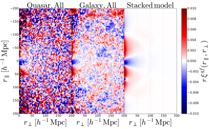
Figure 5.— Measured and best fit MgII - object cross-correlation multiplied by the absolute separation $r=|\vec{r}|$. The color scale is saturated at both negative and positive values in order not to be dominated by the noise and to be the same for the three figures; it is symmetric about zero. Left: Stack of the $15$ correlations involving quasars. Center: Stack of the $15$ correlations involving galaxies. Right: Stack of the $30$ best fit models, when running the combined fit (last line of table 3).

For each of our $30$ cross-correlations we define the effective redshift, $z_{\mathrm{eff}}$, as the weighted mean redshift of object-pixel pairs for bins with $r\in[80,120]\,h^{-1}\,\mathrm{Mpc}$, i.e., in the region where the BAO feature is expected according to our $\Lambda$CDM cosmology. The effective redshift values are given in table 3; they range from $z_{\mathrm{eff}}=0.44$ to $z_{\mathrm{eff}}=1.03$, with an effective redshift for the weighted stack of all cross-correlations: $z_{\mathrm{eff}}=0.59$.

The number of object-pixel pairs in the BAO region, $r\in[80,120]\,h^{-1}\,\mathrm{Mpc}$, varies from $134$ million in the cross-correlation between the Ly$\beta$ forest and quasars up to $36$ billion in the cross-correlation between the Ly$\alpha$ forest and galaxies. Over the $30$ different correlation functions, a total of $170$ billion object-pixel pairs are used in the region where BAO is expected.

4.2. The covariance matrix

The covariance matrix of the cross-correlation is calculated by sub-sampling the data sample similar to the approach in dMdB2017. We divide the sky into HEALPix pixels (Górski et al., 2005) and compute the cross-correlation function in each sub-sample. Using a division of the footprint of figure 1 with $\textit{nside}=32$, we obtain a minimum of $3219$ and a maximum of $3266$ sub-samples for each cross-correlation. Each cross-correlation has $5000$ bins in $(r_{\parallel},r_{\perp})$; the covariance between two of these bins $A$ and $B$ is given by:

$$C_{AB}=\frac{1}{W_{A}W_{B}}\sum\limits_{s}W_{A}^{s}W_{B}^{s}\left[\xi^{s}_{A}\xi^{s}_{B}-\xi_{A}\xi_{B}\right],$$ (10)

where $\xi_{A}^{s}$ and $W_{A}^{s}$ are the cross-correlation and the sum of weights in the sub-sample $s$, respectively, for the bin $A$.

This covariance matrix can be decomposed into two quantities. The diagonal, $C_{AA}$, gives the variance of the bins, and is approximately inversely proportional to the number of pairs and proportional to the variance of the pixel:

$$C_{AA}\sim\frac{c_{A}\left<\delta^{2}\right>}{N^{A}_{\mathrm{pair}}}.$$ (11)

The variance of the pixels $\langle\delta^{2}\rangle$ is of order $0.003$ in all MgII(i) forests and higher in other forests: of order $0.1$ in Ly$\beta$ and Ly$\alpha$ and of order $0.01$ in SiIV and CIV. The parameter $c_{A}$ is the strength of the correlations between different object-pixel pairs. If all pairs are independent, $c_{A}=1$. Since the same pixel is used in different pixel-object pairs, and since pixels are correlated along their line-of-sights, $c_{A}$ is larger than one. The parameter $c_{A}$ is different for each forest - object pair: it is approximately $5$ for correlations involving MgII(i) forests and slightly lower in other forests.

To describe the off-diagonal terms of the covariance matrix, it is convenient to define the correlation matrix:

$$Corr_{AB}=\frac{C_{AB}}{\sqrt{C_{AA}C_{BB}}}.$$ (12)

As with the variance, this correlation matrix is different for each forest - object measurement. Figure 6 displays the primary elements of the correlation matrix for the cross-correlation between quasars and MgII absorption in the MgII(5) forest: $\xi^{\mathrm{QSO},\mathrm{MgII(5)}}$, and for the cross-correlation between galaxies and MgII absorption in the MgII(5) forest: $\xi^{\mathrm{Gal},\mathrm{MgII(5)}}$. The left panel of the figure shows the correlation matrix as a function of $\Delta r_{\parallel}=|r_{\parallel,A}-r_{\parallel,B}|$ for a constant $\Delta r_{\perp}=|r_{\perp,A}-r_{\perp,B}|=0\,h^{-1}~{}\mathrm{Mpc}$. The right panel of the figure presents the correlation in the other direction: as a function of $\Delta r_{\perp}$ at $\Delta r_{\parallel}=0\,h^{-1}~{}\mathrm{Mpc}$. Both correlations drop with increasing separation; however, the correlations decrease faster for quasars than for galaxies. The correlations in the galaxy-forest measurement explain the different patches of the middle panel of figure 5. This slower decrease is explained by the fact that there are around five times as many galaxies as there are quasars, and thus the same pixel is used for an object-pixel pair many more times with galaxies than with quasars.

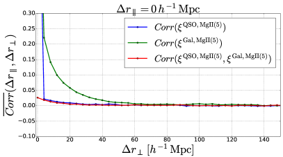
Figure 6.— Correlation matrix $Corr_{AB}$, i.e., the normalized covariance matrix, for the cross-correlation $\xi^{\mathrm{QSO},\mathrm{MgII(5)}}$ (in blue) and for the cross-correlation $\xi^{\mathrm{Gal},\mathrm{MgII(5)}}$ (in green). The red curves are the cross-correlation matrix: the correlation matrix between the two previous cross-correlations. All correlations are given for a mean over all possible pairs within $\Delta r_{\perp}=0\,h^{-1}~{}\mathrm{Mpc}$ (left) and $\Delta r_{\parallel}=0\,h^{-1}~{}\mathrm{Mpc}$ (right) as a function of $\Delta r_{\parallel}$ (left) and $\Delta r_{\perp}$ (right). All correlation matrices vanish for $\Delta r_{\parallel}>150\,h^{-1}~{}\mathrm{Mpc}$.

To limit the noise due to the finite number of sub-samples, we model all the different correlation matrices by taking their mean as a function of $(\Delta r_{\parallel},\Delta r_{\perp})=(|r_{\parallel,A}-r_{\parallel,B}|,|r_{\perp,A}-r_{\perp,B}|)$. This model was validated for the Ly$\alpha$ - quasar cross-correlation in dMdB2017 using different methods of estimating the correlation matrix. Three of the $30$ cross-correlations still have a non-positive definite correlation matrix: galaxy-MgII(8), quasar-MgII(8) and galaxy-MgII(10). We maintain their variance estimates but replace their correlation matrix with the one from the neighboring forest: galaxy-MgII(7), quasar-MgII(7) and galaxy-MgII(9), respectively.

Figure 6 also presents the cross-correlation matrix between the cross-correlation $\xi^{\mathrm{QSO},\mathrm{MgII(5)}}$ and $\xi^{\mathrm{Gal},\mathrm{MgII(5)}}$, defined by:

$$Corr^{q1\,f1,q2\,f2}_{AB}=\frac{C^{q1\,f1,q2\,f2}_{AB}}{\sqrt{C^{q1\,f1}_{AA}C^{q2\,f2}_{BB}}},$$ (13)

where $A$ is a bin of the cross-correlation $\xi^{q1\,f1}$, of covariance $C^{q1\,f1}$, and $B$ is a bin of the cross-correlation $\xi^{q2\,f2}$, of covariance $C^{q2\,f2}$. The cross-covariance is given by:

$$C_{AB}^{q1\,f1,q2\,f2}=\frac{1}{W_{A}W_{B}}\sum\limits_{s}W_{A}^{s}W_{B}^{s}\left[\xi^{s,\,q1\,f1}_{A}\xi^{s,\,q2\,f2}_{B}-\xi^{q1\,f1}_{A}\xi^{q2\,f2}_{B}\right].$$ (14)

Since there are $15$ different forests and $2$ different objects, we have $30$ different cross-correlations and $435$ different cross-covariances. As seen in figure 6, the correlation between the two cross-correlations doesn’t exceed $4\%$ and vanishes at large separations. The amplitude is similar for all $435$ cross-covariances. In this study, we thus neglect this correlation.

4.3. The distortion matrix

The fit of the continuum of equation 2 introduces correlations between pixels from the same forest. The larger the wavelength coverage of a forest, the smaller the correlation. This aspect introduces extra correlation in the 3D pixel-object cross-correlation at large scale. The measured correlation is thus a “distorted” version of the true cross-correlation. The process to compute the distortion matrix, $D_{AA\prime}$, that describes the transformation of the true cross-correlation to the measured cross-correlation is presented in section 4.2 of dMdB2017.

The distortion matrix depends on the length of the forest, the geometry of the survey, and the relative weights of the pixels. We thus compute this matrix for each of the $30$ forest-object pairs. The different MgII(i) forests are shorter than the Ly$\alpha$ forest so their distortion matrix is less diagonal, i.e., the correlation between pixels from the same forest is stronger. For the Ly$\alpha$ forest, the diagonal terms cover the range $0.97<D_{AA\prime}<0.98$ and the off-diagonal terms are $|D_{AA\prime}|<0.022$. For the MgII(i) forests, the diagonal terms cover the range $0.92<D_{AA\prime}<0.96$ and the off-diagonal terms are $|D_{AA\prime}|<0.077$.

5. Fit for cosmological correlations

5.1. Model for the cross-correlations

The model fitting technique used to analyze the 30 different cross-correlations is the same as the one developed in section 5.1 of dMdB2017 and in section 6 of Blomqvist2018. We only give here a brief summary.

Each measured cross-correlation is a combination of three correlations. For correlations involving quasars, they are the quasar-MgII(2796), the quasar-MgII(2804) and the quasar-MgI(2853) cross-correlations. In this analysis, we have defined the redshift of the pixels using the wavelength of the MgII(2796) absorption. The main effect of this operation is to shift the different correlations involving other transitions mostly along the $r_{\parallel}$ direction. These shifts are given by the fiducial cosmology and evolve with redshift. At a redshift $z=0.59$, corresponding to $\lambda=4446\,\mathrm{\AA{}}$ for MgII(2796), the shifts are $\sim 9\,h^{-1}~{}\mathrm{Mpc}{}$ for quasar-MgII(2804) and $\sim 68\,h^{-1}~{}\mathrm{Mpc}{}$ for quasar-MgI(2853), as given in table 2. This effect is taken into account by the “metal distortion matrix” (eqn. 6.18 of Blomqvist2018).

The expected measured signal for each of the 30 object-forest cross-correlations is given by:

$$\widehat{\xi_{A}}=D_{AA^{\prime}}\biggl{[}\xi_{A^{\prime}}^{q,\mathrm{MgII(2796)}}\\ +M_{A^{\prime}B^{\prime}}^{q,\mathrm{MgII(2804)}}\xi_{B^{\prime}}^{q,\mathrm{MgII(2804)}}+M_{A^{\prime}B^{\prime}}^{q,\mathrm{MgI(2853)}}\xi_{B^{\prime}}^{q,\mathrm{MgI(2853)}}\biggr{]},$$ (15)

where the sum is implicit over the repeated bins in $(r_{\parallel},r_{\perp})$, $A^{\prime}$ and $B^{\prime}$, from equation 7. In this equation, $q$ represents one of the two discrete tracers: $q\in\{\mathrm{quasar}$, $\mathrm{galaxy}\}$, $D_{AA^{\prime}}$ is the distortion matrix that models the modification of the correlation-function by the fit of the continuum from equation 2 (sec. 4.3), and $M_{A^{\prime}B^{\prime}}$ is the metal distortion matrix, introduced above.

Each of the three cross-correlation $\xi^{q,m}$ of equation 15 is given by the Fourier transform of the cross-power spectrum:

$$P^{q,m}(\vec{k},z)\propto b_{q}(z)b_{m}(z)\left(1+\beta_{q}\mu_{k}^{2}\right)\left(1+\beta_{m}\mu_{k}^{2}\right)P_{QL}(\vec{k},z,\alpha_{\mathrm{iso}}),$$ (16)

with $m\in\{$MgII(2796), MgII(2804), MgI(2853)$\}$ and with $q\in\{$quasar, galaxy$\}$.

The bias $b_{i}$ and the redshift space distortion (RSD) parameter $\beta_{i}$ are different for each tracer: $i\in\{$quasar, galaxy, MgII(2796), MgII(2804), MgI(2853)$\}$ and evolve with redshift. In this analysis, the three magnesium transitions are treated as a continuum field of absorption; this implies that their bias and RSD parameters are given, following McDonald (2003); Font-Ribera & Miralda-Escudé (2012); Gontcho A Gontcho et al. (2018), by:

$$b_{m}(z)=-\tau_{m}(z)b_{h,m}(z),$$ (17)

and

$$\beta_{m}(z)=\beta_{h,m}(z).$$ (18)

In these two equations, $(b,\beta)_{m}$ are the bias and RSD parameters of the three different magnesium transitions treated as a continuous field, while $(b,\beta)_{h,m}$ are their respective host halos bias and RSD parameter. The averaged optical depth, $\tau_{m}$, is different for each of the three transitions and can evolve with redshift. As explained in the introduction (sec. 1), MgII has a bias much smaller than unity when treated as a transmission field. This is apparent in equation 17. While the halos that host MgII absorption have a bias comparable to that of galaxies, $|b_{h,m}|\sim 1$, the mean optical depth is much smaller than unity: $\tau_{m}\ll 1$. Another way to understand the low bias is to compare the MgII transmission field to that of the Lyman-$\alpha$ forest. The cosmic MgII number density is much lower than that of neutral hydrogen as can be seen in the two spectra of figure 3. Many more absorption lines from hydrogen are visible at wavelengths shorter than the quasar Ly$\alpha$ emission line than from any other metals at wavelengths longer than the quasar Ly$\alpha$ emission line. The bias from metals is therefore much lower than that of Lyman-$\alpha$.

We model the evolution of transmission and halo bias by the following power-law:

$$b_{i}(z)=b_{i}(z_{\mathrm{eff}})\left(\frac{1+z}{1+z_{\mathrm{eff}}}\right)^{\gamma_{i}}.$$ (19)

For quasars we adopt the measured values of the bias at different redshifts in Croom et al. (2005); Shen et al. (2013); Laurent et al. (2016, 2017), and for galaxies in Howlett et al. (2015); Gil-Marín et al. (2016); Zhai et al. (2017). All these results are presented in the left panel of figure 7, after correction for the different assumptions of fiducial cosmology. The two free parameters of equation 19 for both tracers are determined through a fit of those measurements, assuming they are independent:

$$\begin{array}[]{lllllll}b_{\mathrm{quasar}}(z_{\mathrm{eff}}=0.59)=1.24\pm 0.05,\\ \gamma_{\mathrm{quasar}}=1.44\pm 0.08,\\ Corr=-93\%,\\ \\ b_{\mathrm{galaxy}}(z_{\mathrm{eff}}=0.59)=2.07\pm 0.02,\\ \gamma_{\mathrm{galaxy}}=1.33\pm 0.15,\\ Corr=-18\%.\end{array}$$ (20)

Although the galaxies used in this study are more biased than the quasars at the effective redshift $z_{\mathrm{eff}}=0.59$, the redshift evolution for both tracers is compatible. Because of the degeneracies between magnesium and object bias, we fix the galaxy and quasar bias and their evolution as given by equation 20 at the effective redshift of each cross-correlation. We leave free the bias of the three different magnesium transitions, and assume that their redshift evolution is given by the same power-law index as the galaxies and we fix this parameter: $\gamma_{\mathrm{Mg}}=1.33$. This approach corresponds to no evolution, $\gamma_{\tau_{\mathrm{Mg\,m}}}=0$, of their optical depth of equation 17: $\tau_{m}(z)=\tau_{m}$. This assumption has no consequences on the BAO measurement (table 4), but affects the measurement of the magnesium bias. We revisit this point in section 5.4.

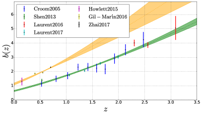
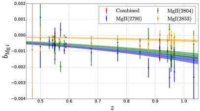
Figure 7.— Bias evolution with redshift. Left: evolution for quasar bias from Croom et al. (2005); Shen et al. (2013); Laurent et al. (2016, 2017), and for galaxies from Howlett et al. (2015); Gil-Marín et al. (2016); Zhai et al. (2017). The green and orange bands indicate the $68\%$ confidence contours of the evolution (eqn. 20) fit to the data point. Right: evolution for the three Mg biases, $b_{i}$, from the results of individual fit to the cross-correlations (first part of table 3). The orange, green and blue bands produce the contours from the fit to all orange, green and blue data points (eqn. 24). The results for the three combined fit to the cross-correlations are given in red ($z_{\mathrm{eff}}\in\{0.55,0.92,0.59\}$, two last parts of table 3).

The RSD parameters for quasars and galaxies are given by the product:

$$b_{i}(z_{\mathrm{eff}})\beta_{i}(z_{\mathrm{eff}})=f(z_{\mathrm{eff}}),$$ (21)

where $f$ represents the linear growth rate of structure. In $\Lambda$CDM cosmology this quantity is approximated by: $f(z)=\Omega_{m}^{0.55}(z)$. As with the bias of objects, we fix $f$ at the effective redshift of the different cross-correlations. The RSD parameter of Mg is highly correlated with the bias, we therefore fix it to be equal to the RSD parameter of galaxies, $\beta_{\mathrm{Mg}}=\beta_{\mathrm{galaxy}}$, for all three transitions. We thus assume that MgII absorbers lie in galaxy halos. Equation 21 also applies to the host halos of the three magnesium transitions. Their optical depth is given by:

$$\tau_{m}(z)=-\frac{(b\beta)_{m}}{f}(z).$$ (22)

The quasi-linear power spectrum $P_{QL}$ of equation 16 (eqn. 6.6 of Blomqvist2018) is computed using CAMB (Lewis et al., 2000) and depends on the BAO parameter: $\alpha_{\mathrm{iso}}$. This parameter acts as an isotropic shift of the BAO wiggles along the wavenumber $k$, corresponding to an isotropic shift of the BAO scale along the direction $r$ of the correlation function (Kirkby et al., 2013). We use a box prior of $\alpha_{\mathrm{iso}}\in[0.5,1.5]$.

The last two relevant parameters to our study are the overall shift of the cross-correlation due to systematic errors in the measurement of quasar and galaxy redshifts ($\Delta r_{\parallel}$: eqn. 6.19 of Blomqvist2018), and the effect of statistical error in redshift measurement and non-linear velocities ($\sigma_{v}$: eqn. 6.10 of Blomqvist2018). Because some of our measurements offer weaker constraining power, for example when using the Ly$\beta$ forest, we add a box prior on the redshift measurement parameter, $\sigma_{v}\in[0,10]\,h^{-1}\,\mathrm{Mpc}$, approximately corresponding to a maximum error of $1000\,\mathrm{km\,s^{-1}}$. This modification affects only poorly measured correlations and has no effect on the measurement of BAO. We remove this prior when performing the combined fit to all $30$ cross-correlations.

5.2. Fit to the cross-correlations

The full model is composed of six free parameters. Four parameters are the main focus of this study: the cosmological BAO parameter, $\alpha_{\mathrm{iso}}$, and the bias parameter of the metal transitions, $b_{\mathrm{MgII(2796)}}$, $b_{\mathrm{MgII(2804)}}$, and $b_{\mathrm{MgI(2853)}}$. The two other nuisance parameters describe the redshift error distribution: the systematic error, $\Delta r_{\parallel}$, and its width, $\sigma_{v}$.

All fits to the cross-correlation functions are done for a separation $r\in\left[10,160\right]\,h^{-1}\,\mathrm{Mpc}$ and for $\mu\in[-1,1]$. We fit each of the 30 different cross-correlations independently and list the results in table 3 at the effective redshift of each measurement. The first part of the table presents the results for all 15 cross-correlations involving galaxies and for all 15 cross-correlations involving quasars. The second part of this table presents the combined fit using all $15$ galaxy cross-correlations to simultaneously constrain the free parameters. We do the same for all quasar cross-correlations. Finally, the third part of the table gives the combined fit to all 30 different cross-correlations.

$\mathrm{Correlation}$	$z_{\mathrm{eff}}$	$\alpha_{\mathrm{iso}}$	$b_{\mathrm{MgII(2796)}}$	$b_{\mathrm{MgII(2804)}}$	$b_{\mathrm{MgI(2853)}}$	$\chi^{2}_{\min{}}/DOF,probability$
[tracer, forest]			$\left[10^{-4}\right]$	$\left[10^{-4}\right]$	$\left[10^{-4}\right]$
$\mathrm{Galaxy,Ly\beta}$	$0.44$	$-$	$\,\,\,-3.7\pm 7.3$	$\,\,\,-6.9\pm 5.2$	$\,\,\,\,\,\,\,5.3\pm 5.5$	$2474.63/(2504-6),p=0.63$
$\mathrm{Galaxy,Ly\alpha}$	$0.44$	$-$	$\,\,\,-2.1\pm 3.5$	$\,\,\,-6.3\pm 3.2$	$\,\,\,\,\,\,\,2.6\pm 2.0$	$2604.66/(2504-6),p=0.067$
$\mathrm{Galaxy,SiIV}$	$0.53$	$-$	$\,\,\,-3.6\pm 1.9$	$\,\,\,-6.6\pm 1.9$	$-1.08\pm 0.68$	$2503.98/(2504-6),p=0.46$
$\mathrm{Galaxy,CIV}$	$0.55$	$-$	$\,\,\,-6.5\pm 1.8$	$\,\,\,-4.9\pm 1.2$	$\,\,\,-2.2\pm 0.78$	$2467.21/(2504-6),p=0.67$
$\mathrm{Galaxy,MgII(1)}$	$0.54$	$-$	$\,\,\,-6.6\pm 1.6$	$\,\,\,-3.1\pm 1.4$	$-0.78\pm 0.90$	$2641.76/(2504-6),p=0.022$
$\mathrm{Galaxy,MgII(2)}$	$0.55$	$-$	$\,\,\,-6.1\pm 2.7$	$\,\,\,-5.2\pm 2.6$	$\,\,\,-1.6\pm 1.0$	$2591.88/(2504-6),p=0.093$
$\mathrm{Galaxy,MgII(3)}$	$0.55$	$-$	$\,\,\,-5.8\pm 1.8$	$\,\,\,-3.6\pm 1.1$	$-0.25\pm 0.73$	$2423.86/(2504-6),p=0.85$
$\mathrm{Galaxy,MgII(4)}$	$0.55$	$-$	$\,\,\,-6.3\pm 2.1$	$\,\,\,-5.6\pm 1.5$	$-1.44\pm 0.89$	$2576.22/(2504-6),p=0.13$
$\mathrm{Galaxy,MgII(5)}$	$0.55$	$-$	$\,\,\,-0.8\pm 3.3$	$-11.4\pm 3.9$	$\,\,\,-3.2\pm 1.3$	$2589.02/(2504-6),p=0.10$
$\mathrm{Galaxy,MgII(6)}$	$0.55$	$-$	$\,\,\,-9.0\pm 2.0$	$\,\,\,-5.5\pm 1.8$	$-2.63\pm 0.96$	$2431.56/(2504-6),p=0.83$
$\mathrm{Galaxy,MgII(7)}$	$0.55$	$-$	$\,\,\,-2.7\pm 2.8$	$\,\,\,-8.1\pm 2.4$	$-1.16\pm 0.86$	$2433.85/(2504-6),p=0.82$
$\mathrm{Galaxy,MgII(8)}$	$0.55$	$-$	$\,\,\,\,\,\,\,1.2\pm 3.7$	$-15.2\pm 3.1$	$\,\,\,-1.8\pm 1.6$	$2375.98/(2504-6),p=0.96$
$\mathrm{Galaxy,MgII(9)}$	$0.57$	$-$	$\,\,\,-7.6\pm 1.9$	$\,\,\,-5.1\pm 1.7$	$-2.28\pm 0.87$	$2542.47/(2504-6),p=0.26$
$\mathrm{Galaxy,MgII(10)}$	$0.57$	$-$	$\,\,\,\,\,\,\,3.6\pm 4.4$	$-19.7\pm 3.4$	$\,\,\,-4.2\pm 1.8$	$2729.40/(2504-6),p=7.2\times 10^{-4}$
$\mathrm{Galaxy,MgII(11)}$	$0.58$	$-$	$\,\,\,-9.4\pm 2.3$	$\,\,\,-5.8\pm 2.7$	$-0.21\pm 0.89$	$2463.90/(2504-6),p=0.68$
$\mathrm{Quasar,Ly\beta}$	$0.47$	$-$	$\,\,\,\,45.0\pm 52.0$	$-78.0\pm 44.0$	$\,\,\,-9.0\pm 36.0$	$2476.67/(2504-6),p=0.62$
$\mathrm{Quasar,Ly\alpha}$	$0.50$	$-$	$\,\,\,-7.0\pm 13.0$	$\,\,\,\,11.4\pm 8.3$	$\,\,\,-2.0\pm 7.9$	$2506.20/(2504-6),p=0.45$
$\mathrm{Quasar,SiIV}$	$0.68$	$-$	$\,\,\,-8.3\pm 7.8$	$-10.9\pm 8.3$	$\,\,\,-4.8\pm 4.4$	$2470.41/(2504-6),p=0.65$
$\mathrm{Quasar,CIV}$	$0.77$	$-$	$-11.3\pm 4.9$	$\,\,\,-4.5\pm 4.0$	$\,\,\,-2.7\pm 2.9$	$2593.62/(2504-6),p=0.089$
$\mathrm{Quasar,MgII(1)}$	$0.85$	$-$	$\,\,\,-6.6\pm 4.6$	$-10.9\pm 3.8$	$\,\,\,-6.6\pm 2.4$	$2637.83/(2504-6),p=0.025$
$\mathrm{Quasar,MgII(2)}$	$0.88$	$-$	$-20.4\pm 6.0$	$\,\,\,-1.8\pm 6.5$	$\,\,\,-5.4\pm 3.5$	$2616.77/(2504-6),p=0.048$
$\mathrm{Quasar,MgII(3)}$	$0.92$	$-$	$\,\,\,-9.3\pm 5.8$	$-10.5\pm 5.2$	$\,\,\,\,\,\,\,0.4\pm 2.7$	$2540.53/(2504-6),p=0.27$
$\mathrm{Quasar,MgII(4)}$	$0.94$	$-$	$\,\,\,-9.7\pm 7.2$	$-10.1\pm 7.0$	$\,\,\,-3.5\pm 3.9$	$2638.80/(2504-6),p=0.025$
$\mathrm{Quasar,MgII(5)}$	$0.95$	$-$	$-26.8\pm 6.4$	$\,\,\,\,\,\,\,3.8\pm 7.1$	$\,\,\,\,\,\,\,0.8\pm 3.8$	$2397.27/(2504-6),p=0.92$
$\mathrm{Quasar,MgII(6)}$	$0.96$	$-$	$-13.5\pm 6.2$	$\,\,\,-8.0\pm 4.8$	$\,\,\,-7.6\pm 4.2$	$2252.95/(2504-6),p=1.00$
$\mathrm{Quasar,MgII(7)}$	$0.96$	$-$	$-15.7\pm 7.2$	$-14.9\pm 7.2$	$\,\,\,-6.7\pm 3.1$	$2413.65/(2504-6),p=0.88$
$\mathrm{Quasar,MgII(8)}$	$0.97$	$-$	$\,\,\,-9.1\pm 5.1$	$-10.2\pm 5.0$	$\,\,\,-4.4\pm 2.8$	$2410.16/(2504-6),p=0.89$
$\mathrm{Quasar,MgII(9)}$	$0.97$	$-$	$-23.0\pm 6.3$	$-11.7\pm 6.2$	$\,\,\,-1.1\pm 2.8$	$2478.24/(2504-6),p=0.61$
$\mathrm{Quasar,MgII(10)}$	$0.96$	$-$	$-13.8\pm 5.4$	$-13.7\pm 6.7$	$\,\,\,-0.3\pm 3.3$	$2598.24/(2504-6),p=0.079$
$\mathrm{Quasar,MgII(11)}$	$1.03$	$-$	$-26.0\pm 14.0$	$\,\,\,-5.7\pm 8.6$	$\,\,\,-3.4\pm 3.6$	$2549.83/(2504-6),p=0.23$
$\mathrm{Galaxy,All}$	$0.55$	$0.982\pm 0.049$	$\,\,\,-6.2\pm 0.55$	$-4.99\pm 0.50$	$-1.08\pm 0.22$	$37916.30/(37560-6),p=0.093$
$\mathrm{QSO,All}$	$0.92$	$1.018\pm 0.052$	$-14.3\pm 1.8$	$\,\,\,-7.9\pm 1.5$	$-2.77\pm 0.85$	$37655.48/(37560-6),p=0.35$
$\mathrm{All,All}$	$0.59$	$0.997\pm 0.037$	$-7.32\pm 0.57$	$-5.28\pm 0.58$	$-1.18\pm 0.21$	$75597.92/(75120-6),p=0.11$

Table 3 Best fit parameters of the BAO and the three Mg biases (for visualization purposes the biases are multiplied by $10^{4}$). The first section lists the results for individual fit to each cross-correlations. The second section gives the results for the combined fit to all $15$ cross-correlations involving galaxies, then to all $15$ cross-correlations involving quasars. The third section presents the results for the combined fit to all $30$ cross-correlations. Since each individual fit doesn’t constrain the BAO parameter, only the results for combined fits are shown.

For cross-correlations involving galaxies, the effective redshifts lie in a relatively small range: from $z_{\mathrm{eff}}=0.44$ to $z_{\mathrm{eff}}=0.58$. For quasars, however, the effective redshifts cover a larger range: from $z_{\mathrm{eff}}=0.47$ to $z_{\mathrm{eff}}=1.03$. The combined fit to all cross-correlations involving galaxies has an effective redshift $z_{\mathrm{eff}}=0.55$, and for quasars it is $z_{\mathrm{eff}}=0.92$. If the bias evolves with redshift, we do not expect its best fit value to agree between bins of different effective redshift.

In this table, the errors are given as the second derivative at the minimum, evaluated at the extrapolated $\Delta\chi^{2}=1$. They do not exactly correspond to direct assessment of $\Delta\chi^{2}=1$, nor to $68.27\%$ of trials. The values of $b_{i}$ are of order $10^{-4}$; for clarity in this table we multiply them by $10^{4}$. The BAO parameter can not be measured significantly in each individual correlation, we therefore present only the best fit results when combining the different measurement: last three lines of table 3.

Among the $30$ individual cross-correlations, $27$ have probabilities $0.0228<p<0.977$, corresponding to two sigma significance, slightly fewer than the $29$ that would be expected from this sample size. The galaxy-MgII(10) cross-correlation has an extremely low probability of $\chi^{2}$. This aspect is explained by the estimation of the correlation-matrix of each of the individual cross-correlation, not to the estimation of variance. As explained in section 4.2, because of numerical issues, we replaced the correlation matrix of galaxy-MgII(8), quasar-MgII(8) and galaxy-MgII(10) by that of their neighboring cross-correlation. This action explains the low probability of $\chi^{2}$ for the galaxy-MgII(10) cross-correlation. This result has little effect on the measurement of the best fit parameters and errors. We test this assumption in the last line of table 4.

We present in the right panel of figure 5 the stack of all the best fit models, after running the combined fit to the 30 cross-correlations. The correlation appears shifted towards positive values of $r_{\parallel}$. This apparent feature is linked to the presence of MgII(2804) at $r_{\parallel}\approx+9\,h^{-1}\,\mathrm{Mpc}$ of MgII(2796) (table 2). The doublet nature is the main source for the asymmetry between the positive and the negative values of $r_{\parallel}$. At $(r_{\parallel},r_{\perp})\approx(+68,0)\,h^{-1}\,\mathrm{Mpc}$, we observe the weaker MgI(2853) correlation.

Figure 8 presents a comparison of the stacked data to the stacked best fit model, for galaxies on the left and quasars on the right. The top panels present the correlation for pairs with $r_{\perp}\approx 0\,h^{-1}\,\mathrm{Mpc}$, i.e., pairs with a small angular separation. These panels highlight the three metal-object correlations. The two elements of the doublet, MgII(2796) and MgII(2804), are blended at $r_{\parallel}\approx 0\,h^{-1}\,\mathrm{Mpc}$. At $r_{\parallel}\approx+68\,h^{-1}\,\mathrm{Mpc}$, we observe the weaker contribution of MgI(2853). These two top panels aim at presenting the fit of the three different correlations of the three different Mg transitions; at our level of precision the BAO feature can not be seen in such figures. The middle panels give the spherically-averaged correlation for both MgII-galaxy and MgII-quasar cross-correlations multiplied by the absolute separation $r$. Finally the bottom two panels show the same two correlations, multiplied by the absolute separation $r^{2}$. In these last two panels we give in red the mean standard fit, in green the mean fit with no BAO feature and in blue a fit of bins in $[40,160]\,h^{-1}~{}\mathrm{Mpc}$ instead of $[10,160]\,h^{-1}~{}\mathrm{Mpc}$. In the fit, the BAO peak can be observed at $r\sim 100\,h^{-1}~{}\mathrm{Mpc}$. In the data, the BAO feature is only weakly statistically detected: $\Delta\chi^{2}=7.25$ (sec. 5.3). Because of the important correlation between different bins of the cross-correlation involving galaxies (figure 6) and the stack of the fit and data, the fit does not go through the points at $r<50\,h^{-1}~{}\mathrm{Mpc}$, however the probability of $\chi^{2}$ is $11\%$. In a similar way, the large scale fluctuations about the fit can be explained by the large correlations of the bins of the correlation function.

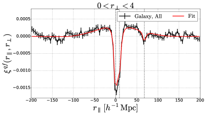
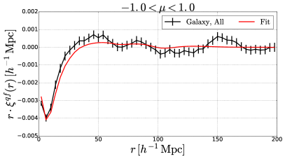
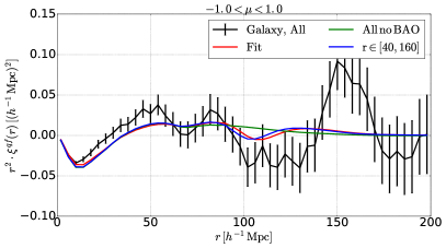
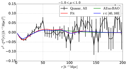
Figure 8.— Comparison between the best fit and the data of the MgII object cross-correlations. Left (right) panels display the stacked best fit and data of all 15 MgII galaxy (quasar) cross-correlations. The top two panels present the cross-correlations for pairs with $r_{\perp}\approx 0\,h^{-1}\,\mathrm{Mpc}$ (small angular separation). The three different Mg correlation maxima are outlined by the gray dashed lines. The middle two panels show the spherically averaged correlation function, multiplied by the absolute separation $r$. The bottom panels show the same correlations, multiplied by the absolute separation $r^{2}$. The standard fit is shown in red, a fit without the BAO feature in green and a fit of bins in $[40,160]\,h^{-1}~{}\mathrm{Mpc}$ instead of $[10,160]\,h^{-1}~{}\mathrm{Mpc}$ in blue.

5.3. Measurement of the baryonic acoustic oscillations

The measurements of BAO in each individual cross-correlation have an average uncertainty of $18\%$. However, the combined fit to all 30 correlations (last part of table 3) leads to isotropic BAO constraints with better than $4\%$ precision. The BAOs correlation with the other five parameters of our model is small: less than $1\%$.

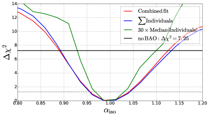
Figure 9.— Result for the BAO parameter from the combined fit to all 30 cross-correlations (last line of table 3). The $\Delta\chi^{2}=\chi^{2}-\chi_{\min}^{2}$ curve for the BAO parameter, $\alpha_{\mathrm{iso}}$, is in red for the combined fit, in blue for the sum of all individual fits, and in green for the median of the $30$ individual fits multiplied by $30$. The gray dashed line indicates $\Delta\chi^{2}=1.28$, corresponding to $\sigma=68.27\%$ confidence levels. The black line is the $\Delta\chi^{2}=7.25$ limit for a model without BAO using a combined fit to all $30$ cross-correlations.

Figure 9 presents the $\Delta\chi^{2}=\chi^{2}-\chi_{\min}^{2}$ curve around the best fit $\alpha_{\mathrm{iso}}$. The red curve gives the result for the combined fit, as shown in the bottom of table 3. The blue curve represents the result for the sum of all $30$ individual fits. The green curve is the median of the $30$ individual fits multiplied by $30$. The three uncertainties yield similar best fit values and errors, thus providing evidence that the individual fits are robust even in the regime of low signal-over-noise ratio. The difference between the median and the combined fit is explained by the large differences in statistics between the $30$ individual fits.

In table 4 of appendix A, we present different systematic tests on the best fit results for $\alpha_{\mathrm{iso}}$ when changing the models or the fitting range for the combined fit to the 30 cross-correlations. No significant changes in the best fit value are detected. We do find one change in the measurement precision by a factor $1.7$ when the amplitude of the BAO peak is introduced as a free parameter. The data are best described with a BAO peak of amplitude $A_{\mathrm{peak}}=2.92\pm 0.82$. The fit using the peak as a free parameter results in $\Delta\chi^{2}=5.5$ from $A_{\mathrm{peak}}=1$, corresponding to a less than $3\sigma$ detection. This enhancement of the BAO peak amplitude could be statistical, linked to spurious signal, or the result of suppressed broadband shape in the measured correlation function. We take the conservative option and keep this parameter fixed to its fiducial value of $A_{\mathrm{peak}}=1$.

To determine if one cross-correlation is driving the results of $\alpha_{\mathrm{iso}}$ and $A_{\mathrm{peak}}$, we compute the combined fit $30$ times removing one of the correlations each time. We perform a similar jackknife, removing also two cross-correlations involving the same forest, producing $15$ different combined fits. The BAO scale and peak size best fit values and errors are compatible with the statistical precision.

The fact that no significant change of the BAO best fit is measured in table 4, or in the jackknife, allows us to assess the different points of the introduction (sec. 1). We discuss these points and their consequences for the Ly$\alpha$ analyses in the conclusion (sec. 6).

The table in the appendix gives, in the last line of the second section, the $\chi^{2}$ for a model with no BAO ($A_{\mathrm{peak}}=0$). When this result is compared to our standard model ($A_{\mathrm{peak}}=1$), it yields $\Delta\chi^{2}=7.25$, shown as a black line in figure 9. This low significance of the BAO peak is consistent with the lack of an evident BAO peak in figure 8. Such a fit is presented in figure 8 by the green line in both bottom panels. A similar significance of the BAO peak is obtained when fitting bins in $[40,160]\,h^{-1}~{}\mathrm{Mpc}$, see last section of table 4. The significance is then: $\Delta\chi^{2}=71171.24-71165.15=6.09$.

As described in dMdB2017, the fit of the BAO parameter is not linear. The link between $\Delta\chi^{2}$ and $\sigma=68.27\%$ must therefore be determined empirically. We determine the relation between BAO measurement precision and the $\chi^{2}$ surface by using $100$ fast Monte-Carlo (fastMC) realizations of our measurements according to our best fit model and covariance matrix. These $100$ fastMC realizations are fit leaving all six parameters free and fixing $\alpha_{\mathrm{iso}}=1$; this selections allows one to efficiently create $100$ realizations of $\Delta\chi^{2}=\chi^{2}_{\alpha_{\mathrm{iso}}=1}-\chi^{2}_{\mathrm{all\,free}}$. We find that $\Delta\chi^{2}=1.28$ does indeed represent $\sigma=68.27\%$ of trials.

The final BAO measurement is generated by the combined fit to all $30$ correlations. After the estimation of the relation between $\Delta\chi^{2}$ and confidence levels, the measurement of the spherically-averaged BAO parameter is:

$$\alpha_{\mathrm{iso}}=0.997\pm 0.047,$$ (23)

where the error represents the $68.27\%$ confidence level. This result is compatible with the cosmology of Planck Collaboration et al. (2016).

For comparison, Alam et al. (2017) measured $\alpha_{\mathrm{iso}}$ with a $1\%$ error in each of the $z=0.32$ and $z=0.57$ bins (their table 9) using the auto-correlation of galaxies from Reid et al. (2016). Ours is the first measurement made at $z<2$ using MgII as a transmission field to measure BAO parameters.

In their study of the CIV absorption in the Ly$\alpha$, SiIV and CIV forests, Blomqvist2018 produced a similar measurement of the BAO parameter at $z=2$: the significance of their BAO peak is given by $\Delta\chi^{2}=3.22$ and their measurement of $\alpha_{\mathrm{iso}}$ is at the $7\%$ level. Only the studies of the Ly$\alpha$ absorption in the Ly$\alpha$ forest from dMdB2017 and Bautista et al. (2017) have a significant measurement of the BAO peak at $z>2$, larger than that presented here, respectively $\Delta\chi^{2}=14$ and $\Delta\chi^{2}=28$. Although the CIV and MgII absorption fields are promising avenues for new BAO measurements, they are not yet able to provide the same precision on the BAO distance scale as the galaxy tracers or Ly$\alpha$ flux-transmission. MgII and CIV do, however, probe the range $1<z<2$ which is currently shot-noise limited in the two-year eBOSS quasar sample; Ata et al. (2018) measures $\alpha_{\mathrm{iso}}=0.993\pm 0.038$ at $z_{\mathrm{eff}}=1.52$.

5.4. Measurement of magnesium bias

For each of our $30$ individual cross-correlations, we have a measurement of the bias, $b_{m}$, of the absorption field of MgII(2796), MgII(2804) and MgI(2853) at their effective redshifts. The results are given in the first part of table 3 and are presented in the right panel of figure 7. This panel gives in blue, green and orange the measurement of MgII(2796), MgII(2804) and MgI(2853), respectively. The red dots are the measurements presented in the last three lines of table 3, i.e., the three different combined fits. At a redshift of $z=0.59$, the three red points are for the combined fit to all of the $30$ cross-correlations.

These three bias measurements are correlated with one another and with $\Delta r_{\parallel}$ and $\sigma_{v}$, but are only marginally correlated with $\alpha_{\mathrm{iso}}$. For the combined fit to all $30$ cross-correlations (last line of table 3), $b_{\mathrm{MgII(2796)}}$ is correlated at the level of $-77\%$ with $b_{\mathrm{MgII(2804)}}$ and $\Delta r_{\parallel}$, at the level of $46\%$ with $\sigma_{v}$, and at the level of $-17\%$ with $b_{\mathrm{MgI(2853)}}$. $b_{\mathrm{MgII(2804)}}$ is correlated at the level of $-89\%$ with $\Delta r_{\parallel}$, at the level of $-64\%$ with $\sigma_{v}$, and at the level of $25\%$ with $b_{\mathrm{MgI(2853)}}$. $b_{\mathrm{MgI(2853)}}$ is correlated at the level of $-25\%$ with $\Delta r_{\parallel}$, and at the level of $-26\%$ with $\sigma_{v}$.

We test for possible systematic errors in our measurement of the bias of the three transitions and present the results in table 4 of appendix A. The second section of the table gives changes in the modeling of the BAO peak. Since the peak is decoupled from the overall correlation function, we observe no changes in the Mg bias measurements under varying assumptions of BAO. In the third section, we modify the model of the fit to the cross-correlation, and in the last section we modify the fitting range. No significant changes in the best fit values of the bias parameters are observed with the exception of three cases.

In the last two lines of the third section, we change the assumption on the number and type of transitions observed: either we assume that MgII(2796) is a singlet and that MgI(2853) is not present ($(b_{\mathrm{MgII(2804)}},b_{\mathrm{MgI(2853)}})=(0,0)$) or we assume that MgII(2804) is a singlet ($b_{\mathrm{MgII(2796)}}=0$). In the first line of the last section of the table we fit only bins with $r_{\parallel}<0$. The effect of these three changes is that the peak produced by the MgII doublet at $r\approx 0\,h^{-1}\,\mathrm{Mpc}$ is modeled as an MgII singlet - object cross-correlation. The resulting effective MgII singlet transition has a bias equal to the sum of the two components in the MgII doublet. This expected value for the effective MgII singlet transition is recovered in the three cases. Thus, these three cases where we observe a significant difference with the bias values of our standard fit are expected, and all yield a bias compatible with $b_{\mathrm{MgII\,singlet}}=-12.6\times 10^{-4}$.

Modeling a doublet as an effective singlet is done in Blomqvist2018 and in Gontcho A Gontcho et al. (2018) for the CIV doublet correlation with the quasar distribution. This choice of analysis gives a measurement of an effective bias of the transition that is the sum of the bias of the two members of the doublet. This approach was motivated by two aspects: the CIV doublet has a smaller separation than the MgII doublet: $2.6$ Å versus $7.2$ Å, and this simplification has no effect on the BAO scale at this level of precision (table 4). This simplification of the MgII transition doublet into an effective singlet has other consequences beyond the bias values. It produces a model that describes the data with less significance. In our study, the standard combined fit has $\chi^{2}=75597.92$, while the fit with only MgII(2804) and MgI(2853) ($b_{\mathrm{MgII(2796)}}=0$) has $\chi^{2}=75649.21$. The difference is $\Delta\chi^{2}=51$, corresponding to more than 5 $\sigma$ significance, for $1$ degree of freedom difference. The effect occurs at small scales and does not bias estimates of the BAO scale.

The other two consequences of this assumption are not given in table 4. First, modeling the doublet as a single line increases the value of $\sigma_{v}$, the parameter representing the statistical error on the redshift of the quasar or galaxies. In our standard fit we measure $\sigma_{v}=0.2\pm 2.0\,h^{-1}\,\mathrm{Mpc}$; when modeling with a single line, $\sigma_{v}=5.26\pm 0.71\,h^{-1}\,\mathrm{Mpc}$. In a similar way, the parameter representing the systematic shift of the cross-correlations due to biased redshift estimates is affected. In our standard fit, we measure $\Delta r_{\parallel}=-0.06\pm 0.43\,h^{-1}\,\mathrm{Mpc}$; when modeling with an effective line, $\Delta r_{\parallel}=4.21\pm 0.23\,h^{-1}\,\mathrm{Mpc}$. All of these aspects demonstrate the importance of modeling the transition properly as a doublet.

We can not identify any major systematic errors in our measurement of the bias for the three Mg transitions. Contrary to the BAO parameter, $\alpha_{\mathrm{iso}}$, the relation between $\Delta\chi^{2}=(1,4)$ and $(68.27\%,95.45\%)$ of trials is linear, and requires no correction for the statistical uncertainty. Using all measurements at each effective redshift from the first section of table 3, and taking into account their correlation matrix, we fit the three bias values at $z_{\mathrm{eff}}=0.59$ and a common redshift evolution parameter:

$$\begin{array}[]{llll}b_{\mathrm{MgII(2796)}}(z=0.59)=(-6.82\pm 0.54)\,\times 10^{-4},\\ b_{\mathrm{MgII(2804)}}(z=0.59)=(-5.55\pm 0.46)\,\times 10^{-4},\\ b_{\mathrm{MgI(2853)}}(z=0.59)=(-1.48\pm 0.24)\,\times 10^{-4},\\ \gamma_{\mathrm{Mg}}=3.36\pm 0.46.\\ \end{array}$$ (24)

The evolution parameter, $\gamma_{\mathrm{Mg}}$, defines the evolution of each bias, $b_{m}$, as given in equation 19. A model with a different evolution for each bias does not improve significantly the fit. The three resulting biases are consistent with the values found when performing a combined fit to all $30$ cross-correlations (last line of table 3). They also are compatible to fitting all $30$ cross-correlations, leaving free $\gamma_{\mathrm{Mg}}$ (table 4). From the third line of the third section of table 4, we see that our baseline assumption of $\gamma_{\mathrm{Mg}}=1.33$ is disfavored at the level of $\Delta\chi^{2}=27$. This result suggests that $\gamma_{\tau_{\mathrm{Mg}}}\neq 0$, i.e., the optical depth of magnesium from the IGM evolves with redshift. This evolution has no consequences on the BAO best fit value. The contribution of the error on the galaxy and quasar biases and redshift evolution parameter from equation 20 is negligible on the result of equation 24.

The results of equation 24 have correlations: $b_{\mathrm{MgI(2853)}}$ is uncorrelated, but $b_{\mathrm{MgII(2796)}}$ is $-19\%$ correlated with $b_{\mathrm{MgII(2804)}}$, and $22\%$ with $\gamma_{\mathrm{Mg}}$; $b_{\mathrm{MgII(2804)}}$ is $22\%$ correlated with $\gamma_{\mathrm{Mg}}$. We present in the right panel of figure 7 the $1\,\sigma$ band in blue, green and orange for the bias value and evolution with redshift.

From equation 22, we can convert each measurement of magnesium transmission bias to a measurement of magnesium optical depth, and obtain the overall redshift evolution:

$$\begin{array}[]{llll}\tau_{\mathrm{MgII(2796)}}(z=0.59)=(3.37\pm 0.25)\,\times 10^{-4},\\ \tau_{\mathrm{MgII(2804)}}(z=0.59)=(2.64\pm 0.21)\,\times 10^{-4},\\ \tau_{\mathrm{MgI(2853)}}(z=0.59)=(0.67\pm 0.11)\,\times 10^{-4},\\ \gamma_{\tau_{\mathrm{Mg}}}=2.07\pm 0.31.\\ \end{array}$$ (25)

6. Summary and conclusions

We measured the cross-correlation between the distribution of quasars and galaxies with the absorption from magnesium-II in quasar spectra. The measurement was performed using all available data from SDSS-I through SDSS-IV, mostly from the BOSS and eBOSS programs. It is the first time that this MgII-object cross-correlation has been investigated on scales sufficiently large to measure the BAO feature. We detect the correlation at high significance.

Our measurement yields a $4.7\%$ precision estimate of the isotropic BAO parameter $\alpha_{\mathrm{iso}}$ at an effective redshift of $z_{\mathrm{eff}}=0.59$. At a similar redshift, the auto-correlation of galaxies from BOSS (Alam et al., 2017) constrains the same parameter with a $1\%$ precision in two redshift bins.

The three magnesium bias parameters are: $b_{\mathrm{MgII(2796)}}(z=0.59)=(-6.82\pm 0.54)\,\times 10^{-4}$, $b_{\mathrm{MgII(2804)}}(z=0.59)=(-5.55\pm 0.46)\,\times 10^{-4}$, and $b_{\mathrm{MgI(2853)}}(z=0.59)=(-1.48\pm 0.24)\,\times 10^{-4}$. Their redshift evolution is characterized by the power-law index: $\gamma_{\mathrm{Mg}}=3.36\pm 0.46$.

This analysis uses the same Python package, picca, used in Ly$\alpha$ forest BAO measurement in BOSS, eBOSS and in the upcoming Dark Energy Spectroscopic Instrument (DESI: DESI Collaboration et al., 2016). This choice allows tests of the Ly$\alpha$ analyses methodology in the low signal, large amount of data regime. The excellent agreement between the best fit model and the data of the MgII - object cross-correlation demonstrates that picca enables fits of complex correlations. For example, the main absorption lines, MgII(2796) and MgII(2804), comprise a doublet, and the other absorption line, MgI(2853), is relatively strong compared to the strongest one, MgII(2796). The fact that the three signatures appear to be properly modeled demonstrates the robustness of the Ly$\alpha$ analyses and its implementation in picca.

This study further demonstrates the robustness of the Ly$\alpha$ analyses, as it was reported in Bautista et al. (2017) and du Mas des Bourboux et al. (2017). We further address three potential sources of systematic errors:

• We define $15$ different forests and treat them independently to measure the absorption from MgII. We find no significant systematic errors on the BAO scale or on other model parameters, indications that the quasar unabsorbed continuum and its variations are correctly modeled.

• The model for the MgII doublet and MgI absorption results in a $\chi^{2}$ with probabilities that indicate that the model correctly describes the data. The three magnesium transitions are well modeled, as shown, e.g., in the two top panels of figure 8. The tests also suggest that the effect of other metals are correctly modeled.

• The two members of the MgII doublet transition at $z=0.59$ each have a bias $\sim 200$ times smaller than that of Ly$\alpha$ at $z=2.4$. This behavior makes our study more susceptible to systematic errors in flux calibration or sky residuals; however, we find no evidence for such errors.

This study also allows one to independently model the effect of the auto-correlation of MgII embedded in the measured Ly$\alpha$ auto-correlation, as it is done for the CIV auto-correlation embedded in the measured Ly$\alpha$ auto-correlation of Bautista et al. (2017).

This study using MgII, and other analyses using CIV (e.g., Blomqvist et al., 2018), open a new window toward measuring the BAO scale at similar redshifts. The completed eBOSS and DESI surveys will provide multiple low-redshift quasars and galaxies necessary to improve the precision on the BAO parameter from this approach.

Appendix A Systematic tests on BAO and magnesium bias

This appendix presents the set of tests on the combined fit to all $30$ different cross-correlations (last row of table 3). We assess the best fit values and errors on BAO and magnesium biases under different assumptions in the model. The results of all these tests are shown in table 4. The impacts of these tests on our analysis are discussed in section 5.3 and 5.4. The results demonstrate that our measurement is robust against different changes in the analysis.

In this table, each row lists the best fit values and errors of $\alpha_{\mathrm{iso}}$, $b_{\mathrm{MgII(2796)}}$, $b_{\mathrm{MgII(2804)}}$, $b_{\mathrm{MgI(2853)}}$ for one of the tests. When a test has extra parameters, we present the best fit values for those parameters in the first column.

The first section of this table (“Std”) recalls the best fit results in the model chosen in this analysis. This entry is a duplicate of the last row of table 3. The other two parameters have best fit values of: $\Delta r_{\parallel}=-0.06\pm 0.43\,h^{-1}~{}\mathrm{Mpc}{}$ and $\sigma_{v}=0.2\pm 2.0\,h^{-1}~{}\mathrm{Mpc}{}$.

The second section of this table presents the results of the tests on the BAO against different models. The first row is the fit to the BAO using a different parametrization of the peak, as a shift along the line-of-sight and across: $(\alpha_{\parallel},\alpha_{\perp})$. In the second row the BAO scale is fixed to its fiducial value: $\alpha_{\mathrm{iso}}=1$. In the third row, we leave free the parameters setting the non-linear broadening of the BAO peak, $(\Sigma_{\parallel},\Sigma_{\perp})$. Finally, in the fourth row we fit for the size of the BAO peak by leaving free the parameter $A_{\mathrm{peak}}$ from its fiducial value and fix it to zero in the last row to get a model without a BAO scale.

The third section of the table presents changes to the model that affect the overall shape of the cross-correlation without modifying the BAO scale. The rows in this section represent various modifications. 1) we leave free the growth-rate of structure, $f$. 2) we leave free the shared redshift-space distortion parameter of the three magnesium transitions, $\beta_{\mathrm{Mg}}$. 3) we leave free the parameter giving the shared redshift evolution of the bias of the three Mg species, $\gamma_{\mathrm{Mg}}$. 4) we allow the parameter giving the systematic redshift error, $\Delta r_{\parallel}$, to be different for galaxies and for quasars. 5) we allow the parameter giving the statistic redshift error and the effect of non-linear quasar velocities, $\sigma_{v}$, to be different for galaxies and for quasars. 6) we replace the Lorentzian smoothing from measurement error of the quasar redshift by a Gaussian smoothing. 7) we fix to zero the two parameters giving the effect of systematic and statistic errors in the measurement of quasar redshift. 8,9) we either model the cross-correlation by a single transition, or model the MgII doublet by an effective MgII singlet.

The last section of the table gives changes to the fitting range or to the data used. In the first two rows we fit either negative or positive values of separation along the line-of-sight, $r_{\parallel}$. In the next three rows, we change the fitting range in absolute separation, $r$. In the sixth line we fit the correlation function in a narrower fitting range, without the BAO feature. The next two lines show the consequences on the fit, when the non-diagonal elements of the covariance matrices are neglected, on the standard fit and on a fit without the BAO peak. Finally, in the last row we remove the galaxy-MgII(8), quasar-MgII(8) and galaxy-MgII(10) cross-correlations where the correlation matrix had to be replaced with a neighboring correlation matrix to be positive definite.

$\mathrm{Analysis}$	$\alpha_{\mathrm{iso}}$	$b_{\mathrm{MgII(2796)}}$	$b_{\mathrm{MgII(2804)}}$	$b_{\mathrm{MgI(2853)}}$	$\chi^{2}_{\min{}}/DOF,probability$
		$\left[10^{-4}\right]$	$\left[10^{-4}\right]$	$\left[10^{-4}\right]$
$\mathrm{Std.}$	$0.997\pm 0.037$	$\,\,\,-7.32\pm 0.57$	$\,\,\,-5.28\pm 0.58$	$-1.18\pm 0.21$	$75597.92/(75120-6),p=0.11$
$(\alpha_{\parallel},\alpha_{\perp})$	$-$	$\,\,\,-7.32\pm 0.57$	$\,\,\,-5.28\pm 0.58$	$-1.18\pm 0.21$	$75597.89/(75120-7),p=0.11$
$(1.009,0.988)\pm(0.075,0.063)$
$\alpha_{\mathrm{iso}}=1$	$1$	$\,\,\,-7.32\pm 0.57$	$\,\,\,-5.28\pm 0.58$	$-1.18\pm 0.21$	$75597.93/(75120-5),p=0.11$
$(\Sigma_{\parallel},\Sigma_{\perp})$	$0.997\pm 0.037$	$\,\,\,-7.29\pm 0.55$	$\,\,\,-5.31\pm 0.55$	$-1.19\pm 0.21$	$75597.90/(75120-8),p=0.11$
$(0.3,0.0)\pm(1.3,1.9)$
$A_{\mathrm{peak}}$	$1.000\pm 0.022$	$\,\,\,-7.29\pm 0.54$	$\,\,\,-5.28\pm 0.53$	$-1.18\pm 0.21$	$75592.41/(75120-7),p=0.11$
$2.92\pm 0.82$
$A_{\mathrm{peak}}=0$	$-$	$\,\,\,-7.30\pm 0.55$	$\,\,\,-5.26\pm 0.55$	$-1.18\pm 0.21$	$75605.18/(75120-5),p=0.10$
$f$	$0.997\pm 0.037$	$\,\,\,\,\,\,-7.3\pm 3.9$	$\,\,\,\,\,\,-5.3\pm 2.7$	$-1.18\pm 0.63$	$75597.92/(75120-7),p=0.11$
$0.79\pm 0.41$
$\beta_{\mathrm{Mg}}$	$0.997\pm 0.036$	$\,\,\,-8.75\pm 0.78$	$\,\,\,-6.04\pm 0.61$	$-1.44\pm 0.25$	$75587.92/(75120-7),p=0.11$
$0.053\pm 0.088$
$\gamma_{\mathrm{Mg}}$	$1.002\pm 0.037$	$\,\,\,-6.89\pm 0.52$	$\,\,\,-5.04\pm 0.48$	$-1.20\pm 0.21$	$75570.81/(75120-7),p=0.12$
$2.81\pm 0.27$
$(\Delta r_{\parallel,\mathrm{galaxy}},\Delta r_{\parallel,\mathrm{quasar}})$	$0.997\pm 0.036$	$\,\,\,-7.35\pm 0.49$	$\,\,\,-5.28\pm 0.45$	$-1.20\pm 0.21$	$75595.70/(75120-7),p=0.11$
$(0.06,-0.64)\pm(0.34,0.51)$
$(\sigma_{v,\mathrm{galaxy}},\sigma_{v,\mathrm{quasar}})$	$0.997\pm 0.037$	$\,\,\,-7.32\pm 0.56$	$\,\,\,-5.28\pm 0.59$	$-1.18\pm 0.22$	$75597.92/(75120-7),p=0.11$
$(0.2,0.1)\pm(2.3,2.7)$
$\sigma_{v}\,\mathrm{Gauss}$	$0.997\pm 0.037$	$\,\,\,-7.30\pm 0.57$	$\,\,\,-5.31\pm 0.59$	$-1.19\pm 0.21$	$75597.90/(75120-6),p=0.11$
$0.5\pm 2.0$
$(\Delta r_{\parallel},\sigma_{v})=(0,0)$	$0.997\pm 0.037$	$\,\,\,-7.26\pm 0.36$	$\,\,\,-5.34\pm 0.26$	$-1.18\pm 0.21$	$75597.96/(75120-4),p=0.11$
$(b_{\mathrm{MgII(2804)}},b_{\mathrm{MgI(2853)}})=(0,0)$	$0.994\pm 0.036$	$-12.98\pm 0.55$	$-$	$-$	$75682.11/(75120-4),p=0.072$
$b_{\mathrm{MgII(2796)}}=0$	$0.997\pm 0.036$	$-$	$-13.08\pm 0.57$	$-1.40\pm 0.29$	$75649.21/(75120-5),p=0.084$
$r_{\parallel}<0$	$1.225\pm 0.076$	$\,\,\,-10.0\pm 1.8$	$\,\,\,-1.2\,\,\,\pm 2.2$	$\,\,\,\,11.6\pm 4.2$	$38225.32/(37560-6),p=0.0074$
$r_{\parallel}>0$	$0.953\pm 0.056$	$\,\,\,-6.84\pm 0.65$	$\,\,\,-5.34\pm 0.65$	$-1.19\pm 0.22$	$37385.31/(37560-6),p=0.73$
$r\in[0,160]$	$0.997\pm 0.037$	$\,\,\,-7.02\pm 0.25$	$\,\,\,-5.54\pm 0.24$	$-1.22\pm 0.21$	$75875.51/(75360-6),p=0.090$
$r\in[40,160]$	$0.996\pm 0.038$	$\,\,\,-7.4\,\,\,\pm 2.8$	$\,\,\,-5.2\,\,\,\pm 2.8$	$-1.40\pm 0.36$	$71165.15/(70620-6),p=0.072$
$r\in[10,180]$	$0.996\pm 0.037$	$\,\,\,-7.38\pm 0.56$	$\,\,\,-5.29\pm 0.59$	$-1.19\pm 0.21$	$96113.97/(95400-6),p=0.050$
$r\in[40,160]+A_{\mathrm{peak}}=0$	$-$	$\,\,\,-8.5\,\,\,\pm 2.9$	$\,\,\,-4.0\,\,\,\pm 2.8$	$-1.40\pm 0.37$	$71171.24/(70620-5),p=0.070$
$\mathrm{only\,diagonal}$	$0.960\pm 0.026$	$\,\,\,-5.76\pm 0.42$	$\,\,\,-4.3\,\,\,\pm 0.40$	$-1.17\pm 0.13$	$76111.28/(75120-6),p=0.0052$
$\mathrm{only\,diagonal}+A_{\mathrm{peak}}=0$	$-$	$\,\,\,-5.72\pm 0.42$	$\,\,\,-4.26\pm 0.40$	$-1.17\pm 0.13$	$76142.83/(75120-5),p=0.0041$
$\mathrm{only\,Pos.Def.}$	$1.004\pm 0.038$	$\,\,\,-7.39\pm 0.53$	$\,\,\,-5.23\pm 0.47$	$-1.22\pm 0.22$	$68070.75/(67608-6),p=0.10$

Table 4 Best fit results for the BAO parameter and the magnesium biases, for the combined fit to all 30 different cross-correlations under different assumptions in the analysis. The first section reproduces the last row of table 3 for comparison. The second section gives changes in the BAO model. The third section gives changes in the cross-correlation model. The last section lists changes in the fitting range. When the analysis has extra free parameters, their best fits are given in the first column in parentheses immediately below the model description.

References

- Abazajian et al. (2009) Abazajian K. N., Adelman-McCarthy J. K., Agüeros M. A., et al., 2009, ApJS, 182, 543
- Abolfathi et al. (2018) Abolfathi B., Aguado D. S., Aguilar G., et al., 2018, ApJS, 235, 42
- Alam et al. (2017) Alam S., Ata M., Bailey S., et al., 2017, MNRAS, 470, 2617
- Albareti et al. (2017) Albareti F. D., Allende Prieto C., Almeida A., et al., 2017, ApJS, 233, 25
- Anderson et al. (2012) Anderson L., Aubourg E., Bailey S., et al., 2012, MNRAS, 427, 3435
- Anderson et al. (2014a) Anderson L., Aubourg É., Bailey S., et al., 2014a, MNRAS, 441, 24
- Anderson et al. (2014b) Anderson L., Aubourg E., Bailey S., et al., 2014b, MNRAS, 439, 83
- Ata et al. (2018) Ata M., Baumgarten F., Bautista J., et al., 2018, MNRAS, 473, 4773
- Bahcall et al. (1993) Bahcall J. N., Bergeron J., Boksenberg A., et al., 1993, ApJS, 87, 1
- Bautista et al. (2017) Bautista J. E., Busca N. G., Guy J., et al., 2017, A&A, 603, A12
- Bautista et al. (2018) Bautista J. E., Vargas-Magaña M., Dawson K. S., et al., 2018, ApJ, 863, 110
- Beutler et al. (2011) Beutler F., Blake C., Colless M., et al., 2011, MNRAS, 416, 3017
- Blake et al. (2011) Blake C., Davis T., Poole G. B., et al., 2011, MNRAS, 415, 2892
- Blanton et al. (2017) Blanton M. R., Bershady M. A., Abolfathi B., et al., 2017, AJ, 154, 28
- Blanton et al. (2005) Blanton M. R., Schlegel D. J., Strauss M. A., et al., 2005, AJ, 129, 2562
- Blomqvist et al. (2018) Blomqvist M., Pieri M. M., du Mas des Bourboux H., et al., 2018, J. Cosmology Astropart. Phys, 5, 029
- Bolton et al. (2012) Bolton A. S., Schlegel D. J., Aubourg É., et al., 2012, AJ, 144, 144
- Busca et al. (2013) Busca N. G., Delubac T., Rich J., et al., 2013, A&A, 552, A96
- Chuang & Wang (2012) Chuang C.-H., Wang Y., 2012, MNRAS, 426, 226
- Cole et al. (2005) Cole S., Percival W. J., Peacock J. A., et al., 2005, MNRAS, 362, 505
- Croom et al. (2005) Croom S. M., Boyle B. J., Shanks T., et al., 2005, MNRAS, 356, 415
- Dawson et al. (2016) Dawson K. S., Kneib J.-P., Percival W. J., et al., 2016, AJ, 151, 44
- Dawson et al. (2013) Dawson K. S., Schlegel D. J., Ahn C. P., et al., 2013, AJ, 145, 10
- Delubac et al. (2015) Delubac T., Bautista J. E., Busca N. G., et al., 2015, A&A, 574, A59
- DESI Collaboration et al. (2016) DESI Collaboration, Aghamousa A., Aguilar J., et al., 2016, ArXiv e-prints
- du Mas des Bourboux et al. (2017) du Mas des Bourboux H., Le Goff J.-M., Blomqvist M., et al., 2017, A&A, 608, A130
- Eisenstein et al. (2011) Eisenstein D. J., Weinberg D. H., Agol E., et al., 2011, AJ, 142, 72
- Eisenstein et al. (2005) Eisenstein D. J., Zehavi I., Hogg D. W., et al., 2005, ApJ, 633, 560
- Font-Ribera et al. (2013) Font-Ribera A., Arnau E., Miralda-Escudé J., et al., 2013, J. Cosmology Astropart. Phys, 5, 018
- Font-Ribera et al. (2014) Font-Ribera A., Kirkby D., Busca N., et al., 2014, J. Cosmology Astropart. Phys, 5, 27
- Font-Ribera & Miralda-Escudé (2012) Font-Ribera A., Miralda-Escudé J., 2012, J. Cosmology Astropart. Phys, 7, 028
- Font-Ribera et al. (2012) Font-Ribera A., Miralda-Escudé J., Arnau E., et al., 2012, J. Cosmology Astropart. Phys, 11, 059
- Gauthier et al. (2009) Gauthier J.-R., Chen H.-W., Tinker J. L., 2009, ApJ, 702, 50
- Gil-Marín et al. (2016) Gil-Marín H., Percival W. J., Brownstein J. R., et al., 2016, MNRAS, 460, 4188
- Gontcho A Gontcho et al. (2018) Gontcho A Gontcho S., Miralda-Escudé J., Font-Ribera A., Blomqvist M., Busca N. G., Rich J., 2018, MNRAS, 480, 610
- Górski et al. (2005) Górski K. M., Hivon E., Banday A. J., et al., 2005, ApJ, 622, 759
- Gunn & Peterson (1965) Gunn J. E., Peterson B. A., 1965, ApJ, 142, 1633
- Gunn et al. (2006) Gunn J. E., Siegmund W. A., Mannery E. J., et al., 2006, AJ, 131, 2332
- Howlett et al. (2015) Howlett C., Ross A. J., Samushia L., Percival W. J., Manera M., 2015, MNRAS, 449, 848
- Khaire et al. (2018) Khaire V., Walther M., Hennawi J. F., et al., 2018, ArXiv e-prints
- Kirkby et al. (2013) Kirkby D., Margala D., Slosar A., et al., 2013, J. Cosmology Astropart. Phys, 3, 024
- Laurent et al. (2017) Laurent P., Eftekharzadeh S., Le Goff J.-M., et al., 2017, J. Cosmology Astropart. Phys, 7, 017
- Laurent et al. (2016) Laurent P., Le Goff J.-M., Burtin E., et al., 2016, J. Cosmology Astropart. Phys, 11, 060
- Lewis et al. (2000) Lewis A., Challinor A., Lasenby A., 2000, ApJ, 538, 473
- Lundgren et al. (2009) Lundgren B. F., Brunner R. J., York D. G., et al., 2009, ApJ, 698, 819
- Lynds (1971) Lynds R., 1971, ApJ, 164, L73
- Mas-Ribas et al. (2017) Mas-Ribas L., Miralda-Escudé J., Pérez-Ràfols I., et al., 2017, ApJ, 846, 4
- McDonald (2003) McDonald P., 2003, ApJ, 585, 34
- Mehta et al. (2012) Mehta K. T., Cuesta A. J., Xu X., Eisenstein D. J., Padmanabhan N., 2012, MNRAS, 427, 2168
- Myers et al. (2015) Myers A. D., Palanque-Delabrouille N., Prakash A., et al., 2015, ApJS, 221, 27
- Noterdaeme et al. (2012) Noterdaeme P., Petitjean P., Carithers W. C., et al., 2012, A&A, 547, L1
- Noterdaeme et al. (2009) Noterdaeme P., Petitjean P., Ledoux C., Srianand R., 2009, A&A, 505, 1087
- Padmanabhan et al. (2012) Padmanabhan N., Xu X., Eisenstein D. J., et al., 2012, MNRAS, 427, 2132
- Pâris et al. (2018) Pâris I., Petitjean P., Aubourg É., et al., 2018, A&A, 613, A51
- Percival et al. (2007) Percival W. J., Cole S., Eisenstein D. J., et al., 2007, MNRAS, 381, 1053
- Percival et al. (2010) Percival W. J., Reid B. A., Eisenstein D. J., et al., 2010, MNRAS, 401, 2148
- Pérez-Ràfols et al. (2015) Pérez-Ràfols I., Miralda-Escudé J., Lundgren B., et al., 2015, MNRAS, 447, 2784
- Pieri (2014) Pieri M. M., 2014, MNRAS, 445, L104
- Pieri et al. (2014) Pieri M. M., Mortonson M. J., Frank S., et al., 2014, MNRAS, 441, 1718
- Planck Collaboration et al. (2016) Planck Collaboration, Ade P. A. R., Aghanim N., et al., 2016, A&A, 594, A13
- Reid et al. (2016) Reid B., Ho S., Padmanabhan N., et al., 2016, MNRAS, 455, 1553
- Ross et al. (2015) Ross A. J., Samushia L., Howlett C., Percival W. J., Burden A., Manera M., 2015, MNRAS, 449, 835
- Ross et al. (2012) Ross N. P., Myers A. D., Sheldon E. S., et al., 2012, ApJS, 199, 3
- Shen et al. (2013) Shen Y., McBride C. K., White M., et al., 2013, ApJ, 778, 98
- Slosar et al. (2013) Slosar A., Iršič V., Kirkby D., et al., 2013, J. Cosmology Astropart. Phys, 4, 26
- Smee et al. (2013) Smee S. A., Gunn J. E., Uomoto A., et al., 2013, AJ, 146, 32
- Xu et al. (2013) Xu X., Cuesta A. J., Padmanabhan N., Eisenstein D. J., McBride C. K., 2013, MNRAS, 431, 2834
- York et al. (2000) York D. G., Adelman J., Anderson Jr. J. E., et al., 2000, AJ, 120, 1579
- York et al. (2006) York D. G., Khare P., Vanden Berk D., et al., 2006, MNRAS, 367, 945
- Zhai et al. (2017) Zhai Z., Tinker J. L., Hahn C., et al., 2017, ApJ, 848, 76
- Zhu et al. (2014) Zhu G., Ménard B., Bizyaev D., et al., 2014, MNRAS, 439, 3139