Isogeometric Analysis for singularly perturbed problems in 1-D: a numerical study

Abstract

We perform numerical experiments on one-dimensional singularly perturbed problems of reaction-convection-diffusion type, using isogeometric analysis. In particular, we use a Galerkin formulation with B-splines as basis functions. The question we address is: how should the knots be chosen in order to get uniform, exponential convergence in the maximum norm? We provide specific guidelines on how to achieve precisely this, for three different singularly perturbed problems.

1 Introduction

We consider second order singularly perturbed problems (SPPs) in one-dimension, of reaction-convection-diffusion type, whose solution contains boundary layers (see, e.g. [8]). The approximation of SPPs has received a lot of attention in the last few decades, mainly using finite differences (FDs) and finite elements (FEs) on layer adapted meshes (see, e.g. [6]). Various formulations and results are available in the literature, both theoretical and computational [6]. One method that has not, to our knowledge, been applied to general SPPs is Isogeometric Analysis (IGA). Since the introduction of IGA by T. R. Hughes et. al. [5], the method has been successfully applied to a large number of problem classes. Even though much attention has been given to convection-dominated problems [1], the method has not been applied, as far as we know, to a typical singularly perturbed problem, such as (3)–(4) ahead.

Our goal in this article is to study the appication of IGA to SPPs and in particular the approximation of the solution to (3)–(4) ahead. We use a Galerkin formulation with B-splines as basis functions and select appropriate knot vectors, such that as the polynomial degree increases, the error in the approximation, measured in the maximum norm, decays exponentially, independently of any singular perturbation parameter(s). This is the analog of performing $p$ refinement in the FEM.

The rest of the paper is organized as follows: in Section 2 we give a brief introduction to IGA, as described in [1]. In Section 3 we present the model problem and its regularity. In Section 4 we give the Galerkin formulation and construct the discrete problem. Finally, Section 5 shows the results of our numerical computations and Section 6 gives our conclusions.

With $I\subset\mathbf{R}$ an interval with boundary $\partial I$ and measure $\left|I\right|$, we will denote by $C^{k}(I)$ the space of continuous functions on $I$ with continuous derivatives up to order $k$. We will use the usual Sobolev spaces $W^{k,m}(I)$ of functions on $\Omega$ with $0,1,2,...,k$ generalized derivatives in $L^{m}\left(I\right)$, equipped with the norm and seminorm $\left\|\cdot\right\|_{k,m,I}$ and $\left|\cdot\right|_{k,m,I}\,$, respectively. When $m=2$, we will write $H^{k}\left(I\right)$ instead of $W^{k,2}\left(I\right)$, and for the norm and seminorm, we will write $\left\|\cdot\right\|_{k,I}$ and $\left|\cdot\right|_{k,I}\,$, respectively. The usual $L^{2}(I)$ inner product will be denoted by $\left\langle\cdot,\cdot\right\rangle_{I}$, with the subscript omitted when there is no confusion. We will also use the space

$$H_{0}^{1}\left(I\right)=\left\{u\in H^{1}\left(I\right):\left.u\right|_{\partial\Omega}=0\right\}.$$

The norm of the space $L^{\infty}(I)$ of essentially bounded functions is denoted by $\|\cdot\|_{\infty,I}$. Finally, the letters $C,c$ will be used for generic positive constants, independent of any discretization or singular perturbation parameters.

2 Isogeometric analysis

In this study we use B-splines as basis functions and follow [1] closely. To this end let $\Xi=\left\{\xi_{1},\xi_{2},...,\xi_{n+p+1}\right\}$ be a knot vector, where $\xi_{i}\in\mathbf{R}$   is the $i^{th}$ knot, $i=1,2,...,N+p+1$, $p$ is the polynomial order and $N$ is the number of basis functions used to construct the B-spline. The numbers in $\Xi$ are non-decreasing and may be repeated, in which case we are talking about a non-uniform knot vector. If the first and last knot values appear $p+1$ times, the knot vector is called open (see [1] for more details). With a knot vector $\Xi$ in hand, the B-spline basis functions are defined recursively, starting with piecewise constants ($p=0$):

$$B_{i,0}(\xi)=\left\{\begin{array}[]{ccc}1&,&\xi_{i}\leq\xi<\xi_{i+1}\\ 0&,&otherwise\end{array}\right..$$

For $p=1,2,...$, they are defined by the Cox-de Boor recursion formula [3, 4]

$$B_{i,p}(\xi)=\frac{\xi-\xi_{i}}{\xi_{i+p}-\xi_{i}}B_{i,p-1}(\xi)+\frac{\xi-\xi_{i}}{\xi_{i+p}-\xi_{i}}B_{i,p-1}(\xi).$$

In Figure 1 we show some of the above B-splines, obtained with the uniform knot vector $\Xi=[0,0.1,0.2...1]$ for various polynomial degrees $p$.

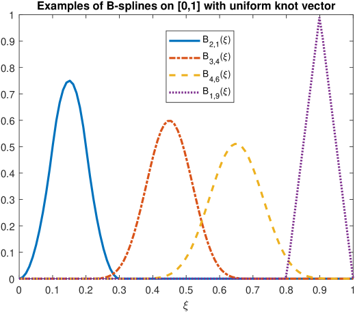
Figure 1: Examples of B-splines using the knot vector $\Xi=[0,0.1,0.2...1]$.

We also mention the recursive formula for obtaining the derivative of a B-spline [1]:

$$\frac{d}{d\xi}B_{i,p}(\xi)=\frac{p}{\xi_{i+p}-\xi_{i}}B_{i,p-1}(\xi)-\frac{p}{\xi_{i+p+1}-\xi_{i+1}}B_{i+1,p-1}(\xi).$$

We will be considering open knot vectors, having possibly repeated entries (other than the endpoints). If we assume we have $\xi_{1},...,\xi_{m}$ distinct knots, each having multiplicity $r_{i}$, then

$$\Xi=[\underset{r_{1\text{ times}}}{\underbrace{\xi_{1},...,\xi_{1}}},\underset{r_{2\text{ times}}}{\underbrace{\xi_{2},...,\xi_{2}}},...,\underset{r_{m\text{ times}}}{\underbrace{\xi_{m},...,\xi_{m}}}]$$

and there holds $\sum_{i=1}^{m}r_{i}=N+p+1$. Since we are using open knots, we have $r_{1}=r_{m}=p+1$. The regularity of the B-spline at each knot $\xi_{i}$ is determined by $r_{i}$, in that the B-spline has $p-r_{i}$ continuous derivatives at $\xi_{i}$. For this reason, we define $k_{i}=p-r_{i}+1$ as a measure of the regularity at the knot $\xi_{i}$ and set $\boldsymbol{k}=[k_{1},...,k_{m}].$ Note that $k_{1}=k_{m}=0$ due to the fact we are using an open knot vector.

B-splines form a partition of unity and they span the space of piecewise polynomials of degree $p$ on the subdivision $\left\{\xi_{1},...,\xi_{m}\right\}$. Each basis function is positive and has support in $[\xi_{i},\xi_{i+p+1}]$. In the sections that follow, we will approximate the solution to the BVP under consideration, using the space

$$S_{\boldsymbol{k}}^{p}=span\left\{B_{k,p}\right\}_{k=1}^{N},$$ (1)

with dimension

$$\mathcal{N}=\dim\left(S_{\boldsymbol{k}}^{p}\right)=mp-\sum_{i=1}^{m}k_{i}.$$ (2)

We point out that we are using a uniform polynomial degree $p$, while we allow for the regularity at each knot to (possibly) vary. A more general approach would be to allow $p$ to vary as well. We will refer to $\mathcal{N}$ as the number of degrees of freedom, DOF.

3 The model problem

We will apply isogeometric analysis to the following model SPP: Find $u$ such that

$$-\varepsilon_{1}u^{\prime\prime}(x)+\varepsilon_{2}b(x)u^{\prime}(x)+c(x)u(x) = f(x)\ \text{in }I=\left(0,1\right),$$ (3)

$$u(0)=u(1) = 0\text{ },$$ (4)

where $0<\varepsilon_{1},\varepsilon_{2}\leq 1$ are given parameters that can approach zero and the functions $b,c,f$ are given and sufficiently smooth. We assume that there exist constants $\beta,\gamma,\rho$, independent of $\varepsilon_{1},\varepsilon_{2},$ such that $\forall\;x\in\overline{I}$

$$b(x)\geq\beta\geq 0\;,\;c(x)\geq\gamma>0\;,\;c(x)-\frac{\varepsilon_{2}}{2}b^{\prime}(x)\geq\rho>0.$$ (5)

The structure of the solution to (3) depends on the roots of the characteristic equation associated with the differential operator. For this reason, we let $\lambda_{0}(x),\lambda_{1}(x)$ be the solutions of the characteristic equation and set

$$\mu_{0}=-\underset{x\in[0,1]}{\max}\lambda_{0}(x)\;,\;\mu_{1}=\underset{x\in[0,1]}{\min}\lambda_{1}(x),$$

or equivalently,

$$\mu_{0,1}=\underset{x\in[0,1]}{\min}\frac{\mp\varepsilon_{2}b(x)+\sqrt{\varepsilon_{2}^{2}b^{2}(x)+4\varepsilon_{1}c(x)}}{2\varepsilon_{1}}.$$ (6)

The values of $\mu_{0},\mu_{1}$ determine the strength of the boundary layers and since $\left|\lambda_{0}(x)\right|<\left|\lambda_{1}(x)\right|$ the layer at $x=1$ is stronger than the layer at $x=0$. Essentially, there are three regimes [6], as shown in Table 1.

Table 1: Different regimes based on the relationship between $\varepsilon_{1}$ and $\varepsilon_{2}$.

		$\mu_{0}$	$\mu_{1}$
convection-diffusion	$\varepsilon_{1}<<\varepsilon_{2}=1$	$1$	$\varepsilon_{1}^{-1}$
convection-reaction-diffusion	$\varepsilon_{1}<<\varepsilon_{2}^{2}<<1\>$	$\varepsilon_{2}^{-1}\>$	$\varepsilon_{2}/\varepsilon_{1}$
reaction-diffusion	$1>>\varepsilon_{1}>>\varepsilon_{2}^{2}$	$\varepsilon_{1}^{-1/2}$	$\varepsilon_{1}^{-1/2}$

We assume that $b,c,f$ are analytic functions satisfying, for some positive constants $\gamma_{f},\gamma_{c},\gamma_{b}$ independent of $\varepsilon_{1},\varepsilon_{2}$, and $\forall\;n=0,1,2,...$

$$\left\|f^{(n)}\right\|_{\infty,I}\leq Cn!\gamma_{f}^{n}\;,\;\left\|c^{(n)}\right\|_{\infty,I}\leq Cn!\gamma_{c}^{n}\;,\;\left\|b^{(n)}\right\|_{\infty,I}\leq Cn!\gamma_{b}^{n}.$$

Then, it was shown in [10] that the solution $u$ to (3), (4) can be decomposed into a smooth part $u_{S}$, a boundary layer part at the left endpoint $u_{BL}^{-}$, a boundary layer part at the right endpoint $u_{BL}^{+}$, and a (negligible) remainder, viz.

$$u=u_{S}+u_{BL}^{-}+u_{BL}^{+}+u_{R},$$

with

$$\left|u_{S}^{(n)}(x)\right|\leq CK^{n}n!,$$

$$\left|\left(u_{BL}^{-}\right)^{(n)}(x)\right|\leq CK_{1}^{n}\mu_{0}^{n}e^{-\ell\mu_{0}x}\;,\;\left|\left(u_{BL}^{+}\right)^{(n)}(x)\right|\leq CK_{2}^{n}\mu_{1}^{n}e^{-\ell\mu_{1}(1-x)},$$

$$\left\|u_{R}\right\|_{\infty,\partial I}+\left\|u_{R}\right\|_{0,I}+\varepsilon_{1}\left\|u_{R}^{\prime}\right\|_{0,I}\leq C\max\{e^{-\delta\varepsilon_{2}/\varepsilon_{1}},e^{-\delta/\varepsilon_{2}}\},$$

for all $x\in\overline{I}$, where the constants $C,K,K_{1},K_{2},\delta>0$ depend only on the data. Figure 2 shows the behavior of the solution to (3)–(4), in all three regimes.

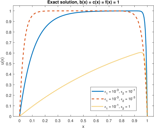
Figure 2: Exact solution for different values of $\varepsilon_{1},\varepsilon_{2}$.

If $\varepsilon_{1},\varepsilon_{2}$ are not small (see Section 5 for precise conditions), then no boundary layers are present and approximating $u$ may be done using a fixed mesh (of say one element) and increasing $p$. (For IGA, the knot vector could simply be $\Xi=[0,...,0,1,...,1]$.) If, on the other hand, $\varepsilon_{1},\varepsilon_{2}$ are small then classical techniques fail and the mesh must be chosen carefully. The challenge lies in approximating the typical boundary layer function $\exp(-x/\varepsilon)$. In the context of FDs and FEs, the mesh points must depend on $\varepsilon$, as is well documented in the literature under the name layer-adapted meshes [6]. We expect something similar to hold for IGA, in the sense that the knot vector must depend on $\varepsilon$. We will illustrate this in Section 5.

4 The Galerkin formulation and the discrete problem

Isogeometric analysis may be combined with a number of formulations; we choose to use Galerkin’s approach, i.e. we multiply (3) by a suitable test function, integrate by parts and use the boundary conditions (4).  The resulting variational formulation reads: Find $u\in H_{0}^{1}\left(I\right)$ such that

$${\mathcal{B}}\left(u,v\right)={\mathcal{F}}\left(v\right)\;\;\forall\;v\in H_{0}^{1}\left(I\right),$$ (7)

where

$${\mathcal{B}}\left(u,v\right)=\varepsilon_{1}\left\langle u^{\prime},v^{\prime}\right\rangle_{I}+\varepsilon_{2}\left\langle bu^{\prime},v\right\rangle_{I}+\left\langle cu,v\right\rangle_{I},\>\>{\mathcal{F}}\left(v\right)=\left\langle f,v\right\rangle_{I}.$$ (8)

The bilinear form ${\mathcal{B}}\left(\cdot,\cdot\right)$ given by (8) is coercive (due to (5)) with respect to the energy norm

$$\left\|u\right\|_{E,I}^{2}:=\varepsilon_{1}\left|u\right|_{1,I}^{2}+\left\|u\right\|_{0,I}^{2},$$

i.e.,

$${\mathcal{B}}\left(u,u\right)\geq\left\|u\right\|_{E,I}^{2}\;\;\forall\;u\in H_{0}^{1}\left(I\right).$$ (9)

Next, we restrict our attention to a finite dimensional subspace $S\subset H_{0}^{1}\left(I\right)$, that will be selected shortly, and obtain the discrete version of (7) as: find $u_{N}\in S$ such that

$${\mathcal{B}}\left(u_{N},v\right)={\mathcal{F}}\left(v\right)\;\;\forall\;v\in S.$$ (10)

The space $S$ is chosen as $S=S_{\boldsymbol{k}}^{p}$ , given by (1).  Thus, we may write the approximate solution as

$$u_{N}=\sum_{k=0}^{N}\alpha_{k}B_{k,p},$$

with $\overrightarrow{\alpha}=[\alpha_{1},...,\alpha_{N}]^{T}$ unknown coefficients, and subsitute in (10) to obtain the linear system of equations

$$\underset{M\in\mathbf{R}^{N\times N}}{\underbrace{\left(\varepsilon_{1}A_{1}+\varepsilon_{2}A_{2}+A_{0}\right)}}\overrightarrow{\alpha}=\overrightarrow{F},$$ (11)

where

$$[A_{1}]_{i,j}=\int_{I}B_{i,p}^{\prime}(\xi)B_{j,p}^{\prime}(\xi)d\xi\;,\;[A_{2}]_{i,j}=\int_{I}B_{i,p}^{\prime}(\xi)B_{j,p}(\xi)d\xi,$$

$$[A_{0}]_{i,j}=\int_{I}B_{i,p}(\xi)B_{j,p}(\xi)d\xi\;,\;[\overrightarrow{F}]_{i=}\int_{I}B_{i,p}(\xi)f(\xi)d\xi,$$

for $i,j=1,...,N.$ The linear system (11) has a unique solution, due to the fact that the coefficient matrix $M$ in (11) is non-singular. To see this, let $0\neq v\in S_{\boldsymbol{k}}^{p}$ be arbitrary and write it as $v=\sum_{k=0}^{N}\beta_{k}B_{k,p}$, with the coefficients $\beta_{k}$ not all zero. From (9), we have

$$0 < \left\|\sum_{k=0}^{N}\beta_{k}B_{k,p}\right\|_{E,I}^{2}\;\leq{\mathcal{B}}\left(\sum_{k=0}^{N}\beta_{k}B_{k,p},\sum_{\ell=0}^{N}\beta_{\ell}B_{\ell,p}\right)$$

$$\leq \sum_{k=0}^{N}\sum_{\ell=0}^{N}\beta_{k}{\mathcal{B}}\left(B_{k,p},B_{\ell,p}\right)\beta_{\ell}=\overrightarrow{\beta}^{T}M\overrightarrow{\beta},$$

which shows that $M$ is positive definite, hence invertible.

We close this section by mentioning that in our implementation of the method, the entries in the matrices in (11), i.e. integrals of B-splines, are computed numerically to any desired accuracy (using MATLAB’s integrate command).

5 Numerical results

In this section we present the results of numerical computations for three examples with known exact solution – this makes our results reliable. We will ‘mimic’ the FEM recommendations for such problems (see, e.g., [10] and the references therein), and select our open knot vector (for the interval $I=(0,1)$) as follows:

With $\mu_{0},\mu_{1}$ given by (6), if $p\mu_{1}^{-1}\geq 1/2$ then

$$\Xi=[\underset{p+1\text{ times}}{\underbrace{0,...,0}},\underset{p+1\text{ times}}{\underbrace{1,...,1}}\}].$$ (12)

If $p\mu_{0}^{-1}<1/2$ then, for reaction-diffusion

$$\Xi=[\underset{p+1\text{ times}}{\underbrace{0,...,0}},p_{\max}\varepsilon^{1/2}_{1},1-p_{\max}\varepsilon^{1/2}_{1},\underset{p+1\text{ times}}{\underbrace{1,...,1}}\}],$$ (13)

for convection-diffusion

$$\Xi=[\underset{p+1\text{ times}}{\underbrace{0,...,0}},1-p_{\max}\varepsilon_{1},\underset{p+1\text{ times}}{\underbrace{1,...,1}}\}],$$ (14)

and for reaction-convection-diffusion

$$\Xi=[\underset{p+1\text{ times}}{\underbrace{0,...,0}},p_{\max}\mu_{0}^{-1},1-p_{\max}\mu_{1}^{-1},\underset{p+1\text{ times}}{\underbrace{1,...,1}}\}],$$ (15)

where $p=1,2,...,p_{\max}$ is the polynomial degree, which we change to improve accuracy. The number of degrees of freedom in each case is given by $DOF=3p$ and we take $p_{max}=10$ for the computations.

We will be measuring the percentage relative error in the maximum norm,

$$Error=100\times\frac{\left\|u-u_{N}\right\|_{\infty,I}}{\left\|u\right\|_{\infty,I}},$$

which we will estimate as follows:

$$Error\approx 100\times\underset{k=1,...,K}{\max}\left|u(x_{k})-u_{N}(x_{k})\right|/\underset{k=1,...,K}{\max}\left|u(x_{k})\right|,$$

where $\left\{x_{k}\right\}_{k=1}^{K}\in I$ are points in $(0,1),$ chosen uniformly in the layer region and outside – we use $K=400$ in each region for our experiments below. We choose to use the maximum norm as an error measure, because the energy norm is ‘not balanced’ for reaction-diffusion problems (see [7] and the references therein).

The examples that follow cover all three regimes, and try to answer the question of how the method performs as $\varepsilon_{1},\varepsilon_{2}\rightarrow 0$. To reduce the error, we increase the dimension of the space by increasing $p$, hence strictly speaking, we are performing $p$-refinement. (In the FEM literature this has been referred to as $hp$-refinment [9].)

Example 1: We consider (3), (4) with $b(x)=0,c(x)=f(x)=1$, which makes the problem reaction-diffusion with $\mu_{0}=\mu_{1}=\varepsilon_{1}^{-1/2}$. Figure 3 shows the percentage relative error measured in the maximum norm, versus the number of degrees of freedom $DOF$ (cf. (2)) in a semi-log scale, and Table 2 lists the errors. The fact that we see straight lines indicates the exponential convergence of the method, while the robustness is verified since the straight lines coincide. We also show, in Figure 4, the results of using a mesh that does not depend on $\varepsilon_{1}$; in particular we use (12), $\varepsilon_{1}=10^{-j},j=1,2,3,6,9,12$ and we increase $p$. As can be seen from the figure, for large $\varepsilon_{1}$ the method yields good results, but as $\varepsilon_{1}\rightarrow 0$, the results deteriorate and we (basically) have no convegence.

Figure 3: Maximum norm convergence for Example 1, using the knot vector (13).

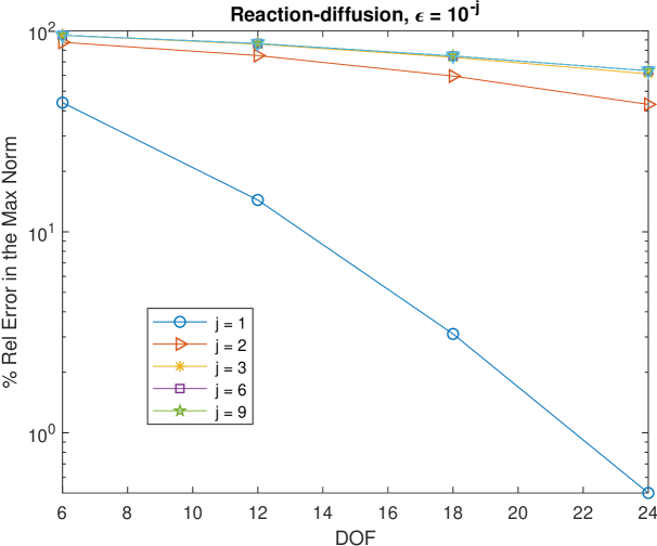
Figure 4: Maximum norm convergence for Example 1, using the knot vector (12).

Table 2: Percentage relative error in the maximum norm for Example 1, using the knot vector (13).

$\varepsilon_{1}:$	$10^{-6}$	$10^{-8}$	$10^{-10}$	$10^{-12}$	$10^{-14}$	$10^{-16}$
$DOF$
6	$44.05$	$44.19$	$44.21$	$44.22$	$44.21$	$44.21$
9	$35.96$	$36.09$	$36.11$	$36.12$	$36.11$	$36.11$
12	$28.48$	$28.78$	$28.81$	$28.82$	$28.82$	$28.82$
$15$	$21.96$	$22.23$	$22.25$	$22.26$	$22.26$	$22.26$
$18$	$15.92$	$16.31$	$16.34$	$16.35$	$16.35$	$16.35$
$21$	$10.75$	$11.01$	$11.04$	$11.04$	$11.04$	$11.04$
$24$	$6.18$	$6.37$	$6.39$	$6.39$	$6.39$	$6.39$
$27$	$2.42$	$2.41$	$2.42$	$2.41$	$2.41$	$2.41$

Example 2: We next consider (3), (4) with $b(x)=c(x)=f(x)=\varepsilon_{2}=1$, which makes the problem convection-diffusion with $\mu_{0}=1,\mu_{1}=\varepsilon_{1}^{-1}.$ In Figure 5 we show the error in the maximum norm versus the number of degrees of freedom, in a semi-log scale, for different values of $\varepsilon_{1}$. The errors are listed in Table 3. Once again we observe robust exponential convergence. The same result as Example 1 is obtained when we use the knot vector (12), hence this is not shown here.

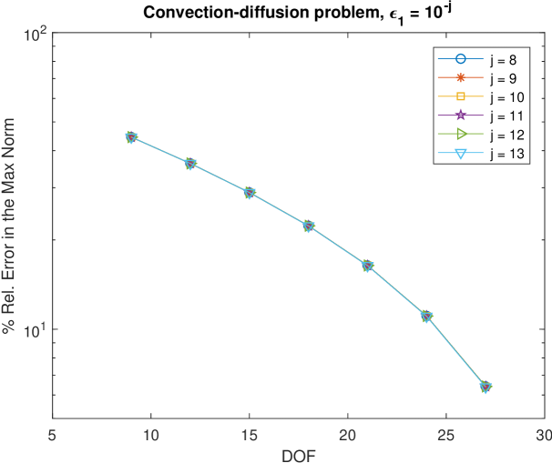
Figure 5: Maximum norm convergence for Example 2, using the knot vector (14).

Table 3: Percentage relative error in the maximum norm for Example 2, using the knot vector (14).

$\varepsilon_{1}:$	$10^{-8}$	$10^{-9}$	$10^{-10}$	$10^{-11}$	$10^{-12}$	$10^{-13}$
$DOF$
$6$	$44.44$	$44.45$	$44.45$	$44.44$	$44.44$	$44.44$
$9$	$36.23$	$36.22$	$36.22$	$36.22$	$36.22$	$36.21$
$12$	$28.91$	$28.90$	$28.91$	$28.91$	$28.90$	$28.89$
$15$	$22.32$	$22.32$	$22.33$	$22.32$	$22.32$	$22.30$
$18$	$16.40$	$16.41$	$16.40$	$16.41$	$16.40$	$16.38$
$21$	$11.08$	$11.09$	$11.08$	$11.08$	$11.08$	$11.05$
$24$	$6.41$	$6.41$	$6.41$	$6.42$	$6.41$	$6.38$
$27$	$2.42$	$2.42$	$2.42$	$2.42$	$2.42$	$2.40$
$30$	$1.92$	$1.92$	$1.92$	$1.93$	$1.93$	$1.95$

Example 3: We finally consider (3), (4) with $b(x)=c(x)=f(x)=1$, and choose the values of $\varepsilon_{1},\varepsilon_{2}$ to satisfy $\varepsilon_{1}<<\varepsilon_{2}^{2}$, so that the problem becomes convection-reaction-diffusion with $\mu_{0}=\varepsilon_{2}^{-1},\mu_{1}=\varepsilon_{2}\varepsilon_{1}^{-1}$. In Figure 6 we show the convergence of the method, measured in the maximum norm, for different values of $\varepsilon_{1},\varepsilon_{2}$. Table 4 shows the actual errors. We observe robust exponential convergence in this final case as well.

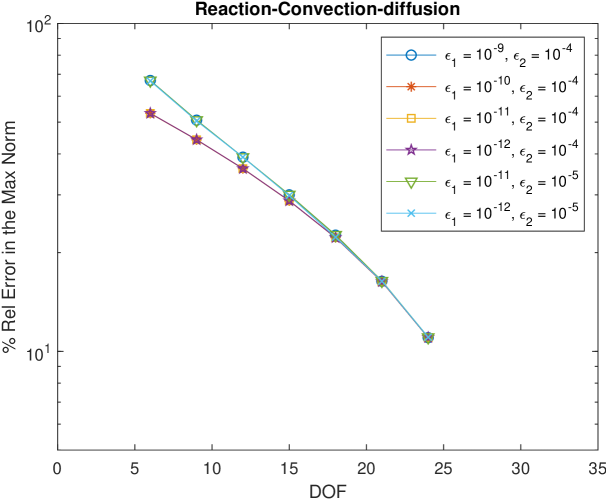
Figure 6: Maximum norm convergence for Example 3, using the knot vector (15).

Table 4: Percentage relative error in the maximum norm for Example 3, using the knot vector (15).

	$\varepsilon_{1}=10^{-9}$	$\varepsilon_{1}=10^{-10}$	$\varepsilon_{1}=10^{-11}$	$\varepsilon_{1}=10^{-12}$	$\varepsilon_{1}=10^{-11}$	$\varepsilon_{1}=10^{-12}$
$DOF$	$\varepsilon_{2}=10^{-4}$	$\varepsilon_{2}=10^{-4}$	$\varepsilon_{2}=10^{-4}$	$\varepsilon_{2}=10^{-4}$	$\varepsilon_{2}=10^{-5}$	$\varepsilon_{2}=10^{-5}$
$6$	$66.98$	$53.17$	$53.18$	$53.20$	$66.97$	$66.74$
$9$	$50.68$	$44.18$	$44.17$	$44.19$	$50.71$	$50.41$
$12$	$39.09$	$36.07$	$36.08$	$36.09$	$39.11$	$39.10$
$15$	$30.01$	$28.77$	$28.78$	$28.79$	$30.05$	$29.84$
$18$	$22.61$	$22.22$	$22.23$	$2.22$	$22.65$	$22.29$
$21$	$16.35$	$16.31$	$16.30$	$16.32$	$16.41$	$16.36$
$24$	$11.00$	$11.02$	$11.03$	$11.01$	$11.05$	$11.04$
$27$	$6.37$	$6.38$	$6.38$	$6.38$	$6.39$	$6.39$
$30$	$2.43$	$2.43$	$2.43$	$2.42$	$2.41$	$2.41$

6 Conclusions

In this article we studied the performance of IGA for one-dimensional reaction-convection-diffusion problems with two small parameters. We observed that if the knot vector is chosen appropriately and depending on the singular perturbation parameter(s), then $p$-refinement yields robust, exponential rates of convergence. The theoretical justification of what we have observed will appear in [11].

As a next step, we intend to study the two-dimensional analogs, as well as higher order operators. In particular, we are investigating the use of IGA to $4^{th}$ order SPPs in two-dimensions, where their use is one of the few available choices for obtaining an approximation, in curvilinear two-dimensional domains.

References

- [1] J. A. Cottrell, T. R. Hughes and Y. Basilevs, Isogeometric Analysis: Toward integration of CAD and FEA, Wiley and Sons (2009).
- [2] L Beirão da Veiga, A. Buffa, J Rivas and G. Sangalli, Some estimates for h-p-k refinement in Isogeometric Analysis, Numer. Math., 118, 271–305 (2011).
- [3] M. G. Cox, The numerical evaluation of B-splines, Technical report, National Physics Laboratory DNAC 4 (1971).
- [4] C. De Boor, On calculation with B-splines, Journal of Approximation Theory, 6, 50–62 (1972).
- [5] T. R. Hughes, J. A. Cottrell and Y. Basilevs, Isogeometric analysis: CAD, finite elements, NURBS, exact geometry and mesh refinement, Comput. Meth. Appl. Mech. Eng., 194 (2005) 4125–4195.
- [6] T. Linß, Layer-adapted meshes for reaction-convection-diffusion problems, Lecture Notes in Mathematics 1985, Springer-Verlag, 2010.
- [7] J. M. Melenk and C. Xenophontos, Robust exponential convergence of hp-FEM in balanced norms for singularly perturbed reaction-diffusion equations, Calcolo, 53 (2016) 105–132.
- [8] H.-G. Roos, M. Stynes, and L. Tobiska. Robust numerical methods for singularly perturbed differential equations, volume 24 of Springer Series in Computational Mathematics. Springer-Verlag, Berlin, second edition, 2008. Convection-diffusion-reaction and flow problems.
- [9] C. Schwab and M. Suri, The p and hp version of the finite element method for problems with boundary layers, Math. Comp., 65 (1996) 1404–1429.
- [10] I. Sykopetritou, An hp finite element method for a second order singularly perturbed boundary value problem with two small parameters, M.Sc Thesis, Department of Mathematics & Statistics, University of Cyprus, 2018.
- [11] C. Xenophontos and I. Sykopetritou, Isogeometric analysis for singularly perturbed problems in 1-D: error estimates, submitted (2019).