Quantum Coherence in a Quantum Heat Engine

Abstract

We identify that quantum coherence is a valuable resource in the quantum heat engine, which is designed in a quantum thermodynamic cycle assisted by a quantum Maxwell’s demon. This demon is in a superposed state. The quantum work and heat are redefined as the sum of coherent and incoherent parts in the energy representation. The total quantum work and the corresponding efficiency of the heat engine can be enhanced due to the coherence consumption of the demon. In addition, we discuss an universal information heat engine driven by quantum coherence. The extractable work of this heat engine is limited by the quantum coherence, even if it has no classical thermodynamic cost. This resource-driven viewpoint provides a direct and effective way to clarify the thermodynamic processes where the coherent superposition of states cannot be ignored.

Keywords: quantum coherence, quantum heat engine and quantum thermodynamics

1 Introduction

Quantum information theory [1, 2] plays a crucial role in thermodynamics [3, 4, 5, 6, 7, 8, 9, 10, 11, 12]. Specifically, the rigorous frameworks for the quantification of quantum coherence [13, 14, 15, 16] and quantum correlations, such as entanglement [17] and discord [18], bring new insights into our understanding about quantum effects in thermodynamics. Those new concepts created from quantum information motivate us to reconsider the physical origin of thermodynamic notions such as work, heat, efficiency of heat engine etc.

On the other hand, remarkable progress of quantum thermodynamics began with the fundamental relations in non-equilibrium statistical mechanics known as the Jarzynski equality [19, 20] or fluctuation theorems [21, 22, 23, 24], which lead to the second law of thermodynamics as a corollary. The Maxwell’s demon [28], as an intermediary, bridges information and thermodynamics [30], such as Landauer’s principle [36, 37] and generalized second laws [24, 25, 26, 27]. All of these support the view that information is a sort of physical existence, contributing to the adaptation of thermodynamics to quantum physics. Existing approaches to quantum thermodynamics are mainly based on operator formalisms [6, 21], which provides a general framework for the thermodynamics of information. Another approach to quantum thermodynamics is path integral formalism [39] based on two-point measurement scheme [20, 40]. This approach provides an effective way to calculate quantum work by utilizing various path integral techniques. However, it is still difficult to figure out where information plays an important role and what kind of information is useful in a specific case, since both classical information and quantum information facilitate thermodynamic processes. It is interesting to explore such problems [3, 38].

As is known, quantum coherence describes the departure of quantum mechanics from the classical realm. It is a natural idea to interpret fundamental thermodynamic notions of quantum system by identifying the behaviour of quantum coherence and combining it with the same basic problem—Maxwell’s demon [28]. Maxwell’s demon has been a fundamental research question and topical issues for statistical mechanics and thermodynamics. Here we consider the object of quantum Maxwell’s demon (QMD) in a quantum heat engine. This type of heat engine assisted by one quantum system has been extensively studied [30, 31, 32]. The other two types of engines are based on the parametric oscillator [33, 34] and the invasive quantum measurement without feedback control [35], respectively. In this paper, we are more concerned about that when the demon is in a superposed state, how its quantum coherence disturbs the whole thermodynamic cycle of the heat engine. The ultimate goal is to explore the behaviour and role of quantum coherence in quantum thermodynamics.

This paper is organized as follows. Firstly, we discuss briefly the resource-theoretic framework of quantum coherence and introduce the QMD with coherence as the control unit in a quantum heat engine. Subsequently, the whole thermodynamic cycle of the heat engine assisted by QMD is studied, and the effects of quantum coherence on the fundamental thermodynamic notions are investigated. In addition, we reinvestigate the information heat engine (IHE) assisted by one memory with coherence, as an universal heat engine driven by quantum coherence. Meanwhile, we calculate the maximum work extractable with the coherence consumption. Finally, more general thermodynamics involving quantum coherence is considered.

2 Quantum Coherence and Quantum Maxwell’s Demon

The rigorous framework for quantifying quantum coherence was first introduced by Baumgratz et al. who proposed four criteria for coherence measures [13]. One well-defined measure is the relative entropy of coherence, which takes the form [13, 14, 15, 16]

$$C_{r}({\rho}):=\min_{\sigma\in\mathcal{I}}S(\rho\|\sigma)=S(\rho_{\mathrm{diag}})-S(\rho),$$ (1)

where $\mathcal{I}$ denotes the set of incoherent states, $S(\rho)=-\mathrm{Tr}{(\rho\ln\rho)}$ is the von Neumann entropy [1] and $\rho_{\mathrm{diag}}$ is the state obtained from $\rho$ by deleting all the off diagonal elements. In the reference basis $|i\rangle$, $\rho_{\mathrm{diag}}$ can be expressed as $\sum_{i}\langle i|\rho|i\rangle|i\rangle\langle i|$. This entropic measure of coherence has a clear physical interpretation and many applications [15]. For instance, quantum coherence can enhance the success probability in Grover search quantum algorithm [45]. In Ref. [46], physical situations have been considered where the resource theories of coherence and thermodynamics play competing roles, especially the creation of quantum coherence comes at a cost of energy. Therefore, coherence can be viewed as a potential quantum resource in quantum physical processes. Exploring more applications of quantum coherence is of wide interests.

To investigate quantum coherence effect in quantum thermodynamics, we introduce a basic problem of statistical mechanics–the paradox of Maxwell’s demon [28], whose role of the information was firstly studied by Szilard [29, 30]. A classical Maxwell’s demon (CMD) can be described as an incoherent state, whereas a quantum Maxwell’s demon (QMD) with off-diagonal elements is in a coherent state, namely

$$\rho_{D}=p_{g}|g\rangle\langle g|+p_{e}|e\rangle\langle e|+F|g\rangle\langle e|+F^{\ast}|e\rangle\langle g|,$$ (2)

where $p_{g}$ and $p_{e}=1-p_{g}$ are the probability distributions in the ground state $|g\rangle$ and excited state $|e\rangle$, respectively. QMD can be viewed as an arbitrary single-qubit system expressed in the Bloch sphere (see Fig. 1). The off-diagonal elements $F$ and $F^{\ast}$ are introduced to embody the quantum coherence. The QMD and its related second law-like equalities (inequalities) have already been experimentally verified by using various systems in recent years [52, 53, 50, 51, 54, 55, 56].

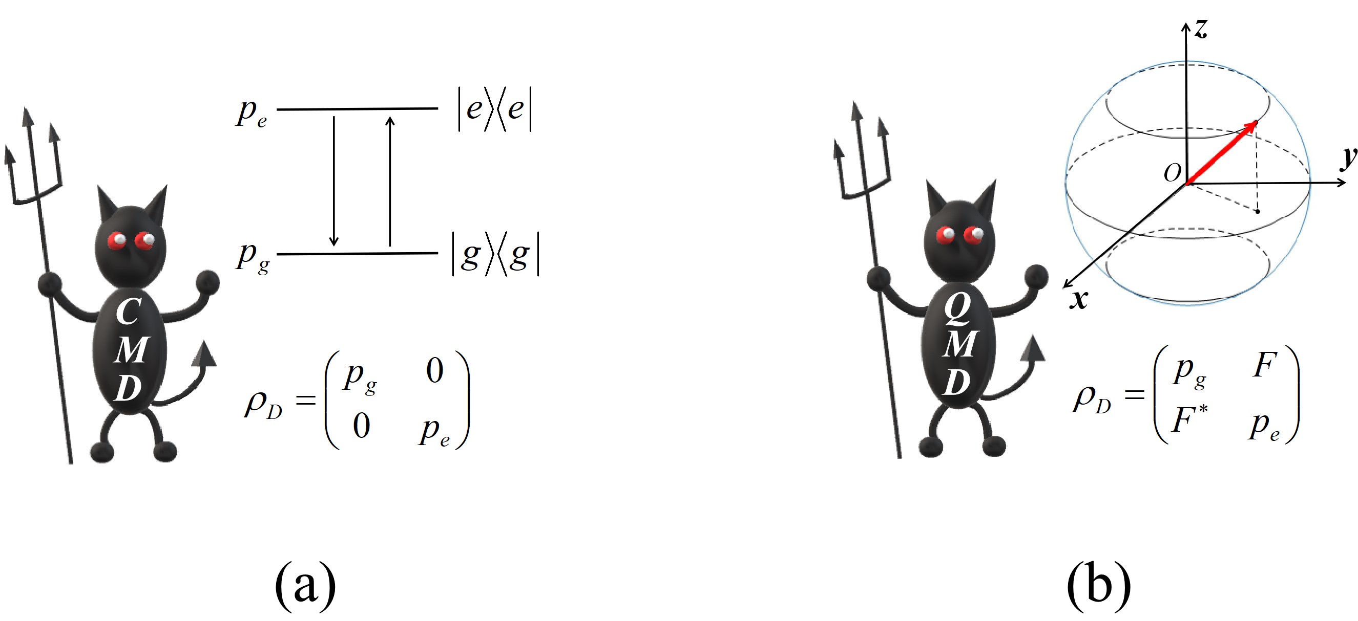
Figure 1: (color online) Classical Maxwell’s demon (CMD) vs quantum Maxwell’s demon (QMD). (a) CMD can be considered as a classical mixture of two definite eigenstates $|g\rangle$ and $|e\rangle$, while QMD with coherence should be preferred to a qubit described in the Bloch sphere, as shown in (b). Here, $p_{g}=(1+z)/2$, $p_{e}=(1-z)/2$, $F=(x-\mathrm{i}y)/2$ and $F^{\ast}=(x+\mathrm{i}y)/2$ are the classical probability distribution of ground state and excited state, and its off-diagonal elements, respectively. Note that $x^{2}+y^{2}+z^{2}\leq 1$, thus $|F|^{2}\leq p_{g}p_{e}$, where the equality is achieved if it is a pure quantum state.

According to Eqs. (1) and (2), the coherence of QMD can be written as

$$C_{r}(\rho_{D})=H(p_{g})-H(\lambda_{+}),$$ (3)

where $H(x)=H(1-x)=-x\ln{x}-(1-x)\ln{(1-x)}$ is the Shannon entropy function [1] and $\lambda_{\pm}=\frac{1}{2}(1\pm\sqrt{(p_{g}-p_{e})^{2}+4|F|^{2}})$ are the eigenvalues of $\rho_{D}$. If we set $\rho_{D}$ as the initial state of QMD in the heat engine $\rho_{D}^{i}$, the initial coherence is exactly in the form of Eq. (3).

In what follows, we will focus on the analysis of the whole quantum thermodynamic cycle assisted by QMD based on quantum Szilard engine (QSE) [43, 49] and reveal the behavior and role of quantum coherence.

3 Quantum Maxwell’s Demon with Coherence Assisted Quantum Thermodynamic Cycle

As a carrier of coherence, QMD is typically designed to drive a QSE [43, 44], which consists of a closed box with definite size $L$ and one system $S$ (such as a single molecule). The demon in our thermodynamic cycle is in contact with a lower temperature heat bath while the system’s bath is at a higher temperature. Although the system is in equilibrium, the QMD is in a nonequilibrium state, as a unit to control expansion. In the cycle, the quantum coherence of the demon is consumed continuously, contributing to the extra work.

The whole thermodynamic cycle is briefly shown in Fig. 2, which is split into five stages: (i) Initial state, (ii) Insertion, (iii) Measurement, (iv) Expansion, and (v) Removal. At the stage of insertion, a wall is isothermally inserted at location $l$. We denote $P_{L}$ as the quantum probability of the system $S$ on the left after insertion , then $P_{R}=1-P_{L}$ is the probability of $S$ on the right. What the QMD should do are performing a global measurement both on the system $S$ and itself (the controlled-NOT operation [47, 48, 49]), and then controlling the expansion of $S$. When the wall is removed and this thermodynamic cycle is completed, $S$ returns to its initial state of equilibrium. In the presence of quantum coherence, it is insufficient to know its diagonal part. Instead, we describe the evolution of the whole system in terms of the full density matrix.

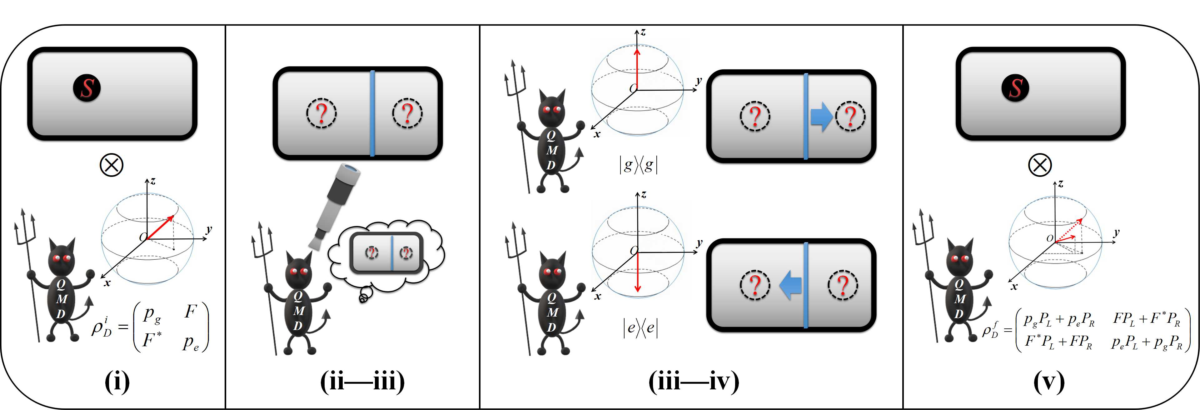
Figure 2: Schematic diagram of the quantum thermodynamic cycle assisted by quantum Maxwell’s demon (QMD). (i) A system $S$ is prepared in a closed box with size $L$ while QMD with coherence is isolated from the box. (ii—iii) A wall, depicted by a vertical blue bar, is isothermally inserted at location $l$. And the measurement is performed later to register the information of the system $S$ into QMD’s memory. (iii—iv) According to the state of the quantum memory, the wall controlled by QMD undergoes a reversible and isothermal expansion until it reaches equilibrium. (v) To complete this thermodynamic cycle, the wall is removed isothermally. At the moment, the state of QMD is overwhelmingly different from the initial state and its coherence has been consumed.

Stage (i): Initial state.— Initially, the system $S$, prepared in a closed box with size $L$, contacts with the reservoir at temperature $T=(k_{\text{B}}\beta)^{-1}$ so that it is in equilibrium. With the initial Hamiltonian $H_{S}=\sum_{n}E_{n}(L)|\psi_{n}(L)\rangle\langle\psi_{n}(L)|$, the density matrix of the initial state of the total system can be written as a product state

$$\begin{split}\rho^{i}&=\rho^{i}_{S}\otimes\rho^{i}_{D}\\ &=\sum_{n}\frac{e^{-\beta E_{n}(L)}}{Z(L)}|\psi_{n}(L)\rangle\langle\psi_{n}(L)|\otimes\rho^{i}_{D},\end{split}$$ (4)

where $Z(L)=\sum_{n}e^{-\beta E_{n}(L)}$, $E_{n}(L)$ and $|\psi_{n}(L)\rangle$ are the partition function, $n$-th eigenenergy and eigenstate of the system $S$ in this box with size $L$. Here, the initial density matrix of QMD, namely $\rho_{D}^{i}$ takes the form of Eq. (2).

The system $S$ will always be in the isothermal process with the reservoir, leading to its thermalization so that all the coherence among energy levels vanishes [43]. Even so, it is necessary to describe the dynamics of the total system in terms of the full density matrix, because our QMD with off-diagonal elements is still coherent at another temperature $T_{D}=(k_{\text{B}}{\beta_{D}})^{-1}$.

Here we emphasize that our discussion doesn’t depend on a specific model. For instance, the box doesn’t have to be an infinite potential well model, i.e., the eigenenergies and eigenfunctions of the system $S$ are $E_{n}(L)=\hbar^{2}\pi^{2}n^{2}/(2mL^{2})$ and $\langle x|\psi_{n}(L)\rangle=\sqrt{2/L}\sin(\pi nx/L)$, where the quantum number $n$ ranges from $1$ to $\infty$.

Stage (ii): Insertion.— After preparing initial state, a wall is then isothermally inserted at a certain position $l$. In the classical situation, the position of the system $S$ is definite, so either it is on the left side or stay on the right side, while in the quantum case the system is simultaneously on both sides of the wall, until its location is determined by the measurement of the observer. Therefore, when the wall insertion is completed, the total density matrix can be expressed as a mixture, namely

$$\rho^{\text{ins}}=[P_{L}\rho^{L}(l)+P_{R}\rho^{R}(L-l)]\otimes\rho^{i}_{D},$$ (5)

where $\rho^{L}(l)=\sum_{n}\frac{e^{-\beta E_{n}(l)}}{Z(l)}|\psi_{n}^{L}(l)\rangle\langle\psi_{n}^{L}(l)|$ and $\rho^{R}(L-l)=\sum_{n}\frac{e^{-\beta E_{n}(L-l)}}{Z(L-l)}|\psi_{n}^{R}(L-l)\rangle\langle\psi_{n}^{R}(L-l)|$ are the independent densities of $S$ on the left and right sides, $P_{L}=Z(l)/[Z(l)+Z(L-l)]$ and $P_{R}=1-P_{L}$ are the corresponding quantum probabilities, which differ from the classical probabilities $P_{L}^{\text{classical}}=l/L$ and $P_{R}^{\text{classical}}=(L-l)/L$ [49]. In this stage, QMD is still out of work, which is the same as CMD. And because the system $S$ has no coherence, thus the results (work, heat, etc.) in this stage only relate with diagonal part of $S$, as in the case of no coherence in Ref. [43].

Stage (iii): Measurement.— Now the demon will perform a global measurement, which can be described by the controlled-NOT operation [48, 49], namely

$$\begin{split}U&=\sum_{n}[|\psi_{n}^{L}(l)\rangle\langle\psi_{n}^{L}(l)|\otimes(|g\rangle\langle g|+|e\rangle\langle e|)\\ &\quad+|\psi_{n}^{R}(L-l)\rangle\langle\psi_{n}^{R}(L-l)|\otimes(|e\rangle\langle g|+|g\rangle\langle e|)].\end{split}$$ (6)

It is easy to verify that $U$ is a unitary operator, which is different from the positive operator valued measure (POVM) in previous discussions [58, 59, 60]. Here, the physical process corresponding to $U$ is that the demon will keep the original state if the system $S$ with $n$ levels is on the left side, while the demon flips its state when $S$ is on the right. After this operation, the total density matrix is given by

$$\begin{split}\rho^{\text{mea}}&=U\rho^{\text{ins}}U^{\dagger}\\ &=P_{L}\rho^{L}(l)\otimes(p_{g}|g\rangle\langle g|+p_{e}|e\rangle\langle e|+F|g\rangle\langle e|+F^{\ast}|e\rangle\langle g|)\\ &\quad\!+\!P_{R}\rho^{R}(L-l)\otimes(p_{e}|g\rangle\langle g|+p_{g}|e\rangle\langle e|+F^{\ast}|g\rangle\langle e|+F|e\rangle\langle g|)\\ &=[p_{g}P_{L}\rho^{L}(l)\!\!+\!\!p_{e}P_{R}\rho^{R}(L\!-\!l)]\!\otimes\!|g\rangle\langle g|\!\!+\!\![p_{e}P_{L}\rho^{L}(l)\!\!+\!\!p_{g}P_{R}\rho^{R}(L\!-\!l)]\!\otimes\!|e\rangle\langle e|\\ &\quad\!\!+\!\![F\!P_{L}\rho^{L}(l)\!\!+\!\!F^{\ast}\!P_{R}\rho^{R}(L\!-\!l)]\!\otimes\!|g\rangle\langle e|\!\!+\!\![F^{\ast}\!P_{L}\rho^{L}(l)\!\!+\!\!F\!P_{R}\rho^{R}(L\!-\!l)]\!\otimes\!|e\rangle\langle g|,\end{split}$$ (7)

which means QMD is now correlated with the system $S$, contributing to the work to the outside.

Compared with CMD, QMD seem to be “blurry-eyed”, so that it can’t exactly distinguish which side the system $S$ stays on. In the limits of $F\rightarrow 0$ and $T_{D}\rightarrow 0$, $\rho^{\text{mea}}\rightarrow P_{L}\rho^{L}(l)\otimes|g\rangle\langle g|+P_{R}\rho^{R}(L-l)\otimes|e\rangle\langle e|$, which implies that QMD is “cured”, i.e., its ground state $|g\rangle$ corresponds to the system $S$ on the left and vice versa, as the case of CMD.

For registering the information of the system $S$ into QMD’s memory, the outside agent have to do work on the total system in this process, leading to the change of the total internal energy. The mean value of this work, namely $\langle W_{\text{mea}}\rangle=\mathrm{Tr}[(H_{S}\!+\!H_{D})(\rho^{\text{mea}}\!-\!\rho^{\text{ins}})]=P_{R}(p_{g}-p_{e})\Delta$, has nothing to do with the off-diagonal elements, because the flip of off-diagonal part makes no contribution to the change of internal energy. However, the off-diagonal part has affected the total density matrix, giving rise to a more complex form about entropy and heat as the following discussions. Here, $H_{S}$ and $H_{D}$ are the Hamiltonian of the system and the demon, respectively. We assume that the demon is a two-level system so that $H_{D}=E_{g}|g\rangle\langle g|+E_{e}|e\rangle\langle e|$ and $\Delta=E_{e}-E_{g}$.

Stage (iv): Expansion.— In this stage, the expansion of the system $S$ is slowly enough to ensure the process reversible and isothermal, which is controlled by QMD according to its memory. The wall will be allowed to move to the right side at a final position $l_{g}$ if QMD is in the ground state and move to the right side at a final position $l_{e}$ if the demon is in the excited state (see intuitively in Fig. 2 (iii—iv)). In accordance with the above analysis, the evolution operator of the controlled expansion can be mathematically constructed as

$$\begin{split}O_{\text{exp}}&\!=\!\!\sum_{n}\!\textstyle\Bigg{\{}\!\bigg{[}\!\sqrt{\!\frac{P_{n}(l_{g})}{P_{n}(l)}}|\psi_{n}^{L}(l_{g})\rangle\langle\psi_{n}^{L}(l)|\!+\!\!\sqrt{\!\frac{P_{n}(L-l_{g})}{P_{n}(L-l)}}|\psi_{n}^{R}(L\!-\!l_{g})\rangle\langle\psi_{n}^{R}(L\!-\!l)|\bigg{]}\!\!\otimes\!|g\rangle\langle g|\\ &\quad+\!\textstyle\bigg{[}\!\sqrt{\!\frac{P_{n}(l_{e})}{P_{n}(l)}}|\psi_{n}^{L}(l_{e})\rangle\langle\psi_{n}^{L}(l)|\!+\!\sqrt{\!\frac{P_{n}(L-l_{e})}{P_{n}(L-l)}}|\psi_{n}^{R}(L\!-\!l_{e})\rangle\langle\psi_{n}^{R}(L\!-\!l)|\bigg{]}\!\!\otimes\!|e\rangle\langle e|\!\Bigg{\}},\end{split}$$ (8)

where $P_{n}(x)=\frac{e^{-\beta E_{n}(x)}}{Z(x)}$. We thus obtain the total density matrix after expansion:

$$\begin{split}\rho^{\text{exp}}&\!=O_{\text{exp}}\rho^{\text{mea}}O_{\text{exp}}^{\dagger}\\ &=\!\big{[}p_{g}P_{L}\rho^{L}(l_{g}\!)\!\!+\!p_{e}P_{R}\rho^{R}(L\!\!-\!\!l_{g}\!)\big{]}\!\otimes\!|g\rangle\langle g|\!\!+\!\!\big{[}p_{e}P_{L}\rho^{L}(l_{e}\!)\!\!+\!p_{g}P_{R}\rho^{R}(L\!\!-\!\!l_{e})\big{]}\!\otimes\!|e\rangle\langle e|\\ &\quad+\big{[}FP_{L}\rho^{L}_{l_{g},l_{e}}+F^{\ast}P_{R}\rho^{R}_{l_{g},l_{e}}\big{]}\otimes|g\rangle\langle e|+\big{[}F^{\ast}P_{L}\rho^{L}_{l_{e},l_{g}}+FP_{R}\rho^{R}_{l_{e},l_{g}}\big{]}\otimes|e\rangle\langle g|,\end{split}$$ (9)

where $\rho^{L}(l_{g})\!=\!\sum_{n}\!P_{n}(l_{g})|\psi_{n}^{L}(l_{g})\rangle\langle\psi_{n}^{L}(l_{g})|$ and $\rho^{R}(l_{e})\!=\!\sum_{n}\scriptstyle\!P_{n}(l_{e})|\psi_{n}^{R}(l_{e})\rangle\langle\psi_{n}^{R}(l_{e})|$ are the post-expansion densities controlled by the diagonal parts $|g\rangle\langle g|$ and $|e\rangle\langle e|$, respectively. Similarly, the items $\rho^{L}_{l_{g},l_{e}}\!=\!\sum_{n}\scriptstyle\!\sqrt{P_{n}(l_{g})P_{n}(l_{e})}|\psi_{n}^{L}(l_{g})\rangle\langle\psi_{n}^{L}(l_{e})|$ and $\rho^{R}_{l_{g},l_{e}}\!=\!\sum_{n}\scriptstyle\!\sqrt{P_{n}(L\!-\!l_{g})P_{n}(L\!-\!l_{e})}|\psi_{n}^{R}(L\!-\!l_{g})\rangle\langle\psi_{n}^{R}(L\!-\!l_{e})|$ in Eq. (9) can be viewed as the post-expansion densities controlled by the off-diagonal part $|g\rangle\langle e|$, whereas $\rho^{L}_{l_{e},l_{g}}\!=\!\sum_{n}\scriptstyle\sqrt{P_{n}(l_{e})P_{n}(l_{g})}|\psi_{n}^{L}(l_{e})\rangle\langle\psi_{n}^{L}(l_{g})|$ and $\rho^{R}_{l_{e},l_{g}}\!=\!\sum_{n}\scriptstyle\sqrt{P_{n}(L\!-\!l_{e})P_{n}(L\!-\!l_{g})}|\psi_{n}^{R}(L\!-\!l_{e})\rangle\langle\psi_{n}^{R}(L\!-\!l_{g})|$ are controlled by $|e\rangle\langle g|$.

In classical physics, the system must be on one side of the wall with another side empty after insertion, thus the wall is doomed to be moved to an end boundary of the box due to expansion. In contrast, quantum system can be simultaneously on both sides of the wall, thus the equilibrium position is somewhere in the box rather than the boundary. The condition of equilibrium, in mechanics, is that the wall has equal and opposite forces on the two sides, i.e. $F^{L}_{\text{eq}}=F^{R}_{\text{eq}}$.

Stage (v): Removal.— For purpose of the thermodynamic cycle, the system $S$ must be reset to its own initial state, i.e. $\rho^{i}_{S}=\sum_{n}\frac{e^{-\beta E_{n}(L)}}{Z(L)}|\psi_{n}(L)\rangle\langle\psi_{n}(L)|$. The corresponding physical process is the wall inserted on the stage (ii) will be removed and all the ensembles of the system $S$ will evolve into $\rho^{i}_{S}$, namely

$$\rho^{\text{rem}}=\sum_{n}\frac{e^{-\beta E_{n}(L)}}{Z(L)}|\psi_{n}(L)\rangle\langle\psi_{n}(L)|\otimes\rho_{D}^{f}.$$ (10)

where

$$\begin{split}\rho_{D}^{f}&=\big{[}(p_{g}P_{L}+p_{e}P_{R})|g\rangle\langle g|+(p_{e}P_{L}+p_{g}P_{R})|e\rangle\langle e|\\ &\quad+(FP_{L}+F^{\ast}P_{R})|g\rangle\langle e|+(F^{\ast}P_{L}+FP_{R})|e\rangle\langle g|\big{]}.\end{split}$$ (11)

In analogy with Eq. (8), we can also construct an operation $O_{\text{rem}}$ to obtain Eq. (10), i.e., $\rho^{\text{rem}}=O_{\text{rem}}\rho^{\text{exp}}O_{\text{rem}}^{\dagger}$ with

$$\begin{split}O_{\text{rem}}&\!=\!\sum_{n}\!\textstyle\Bigg{\{}\bigg{[}\!\sqrt{\!\frac{P_{n}(L)}{P_{n}(l_{g})}}|\psi_{n}(L)\rangle\langle\psi_{n}^{L}(l_{g})|\!+\!\sqrt{\!\frac{P_{n}(L)}{P_{n}(L-l_{g})}}|\psi_{n}(L)\rangle\langle\psi_{n}^{R}(L\!-\!l_{g})|\bigg{]}\!\!\otimes\!|g\rangle\langle g|\\ &\quad+\!\textstyle\bigg{[}\!\sqrt{\!\frac{P_{n}(L)}{P_{n}(l_{e})}}|\psi_{n}(L)\rangle\langle\psi_{n}^{L}(l_{e})|\!+\!\sqrt{\!\frac{P_{n}(L)}{P_{n}(L-l_{e})}}|\psi_{n}(L)\rangle\langle\psi_{n}^{R}(L-l_{e})|\bigg{]}\!\!\otimes\!|e\rangle\langle e|\Bigg{\}}.\end{split}$$ (12)

Here we emphasize that the system $S$ has been reset to thermal equilibrium state with no coherence, but this is not the requirement for QMD. The state of QMD remains coherent, but obviously it’s much less coherent than it was at the beginning. This implies that the coherence consumption may be a direct linkage to work and heat in the whole thermodynamic cycle, as discussed below.

4 Enhancing Efficiency via Coherence Consumption of Quantum Maxwell’s Demon

What we have talked above is the evolution of state of the total system. Because of the coherence, it is insufficient to know its diagonal part. Instead, we describe the evolution of our system in terms of the full density matrix, which is split into five, namely Stage (i-v). As seen in the follows, this approach is in support of studying what we are more concerned, i.e., whether the efficiency of this quantum thermodynamics cycle could be enhanced due to the coherent QMD.

First of all, let us calculate the change of total internal energy $\langle\Delta E_{\text{tot}}\rangle$ by taking $\rho^{\text{rem}}$ as the final density $\rho^{f}$ at the end of this thermodynamics cycle. Focusing on the initial and final states, we can obtain

$$\langle\Delta E_{\text{tot}}\rangle=\langle E_{f}\rangle-\langle E_{i}\rangle=\mathrm{Tr}\big{[}(\rho^{f}-\rho^{i})(H_{S}+H_{D})\big{]}=P_{R}(p_{g}-p_{e})\Delta,$$ (13)

where $H_{D}=E_{g}|g\rangle\langle g|+E_{e}|e\rangle\langle e|$ is the demon’s Hamiltonian and $\Delta=E_{e}-E_{g}$ is the gap of the two levels of QMD. Here, the result is independent of $H_{S}$, namely the form of the Hamiltonian of the system $S$ is inessential during the cycle. Note that $\langle\Delta E_{\text{tot}}\rangle=\langle W_{\text{mea}}\rangle$, i.e., the change of total internal energy merely results from the work done by the outside agent during measurement, as what mentioned before. Eq. (13) also confirms the fact that the change of internal energy does not involve the off-diagonal part at all.

Another important thermodynamic quantity is the total heat $\langle Q_{\text{tot}}\rangle$ absorbed from the outside, which is associated with the total entropy change due to the reversibility, namely

$$\begin{split}\langle Q_{\text{tot}}\rangle&\!=\!k_{\text{B}}T\big{[}S(\rho^{f})-S(\rho^{i})\big{]}\\ &\!=\!k_{\text{B}}T\!\bigg{[}S\textstyle\Big{(}\!\sum_{n}\!\frac{e^{-\beta E_{n}(L)}}{Z(L)}|\psi_{n}(L)\rangle\langle\psi_{n}(L)|\!\otimes\!\rho_{D}^{f}\!\Big{)}\!-\!S\Big{(}\!\sum_{n}\!\frac{e^{-\beta E_{n}(L)}}{Z(L)}|\psi_{n}(L)\rangle\langle\psi_{n}(L)|\!\otimes\!\rho_{D}^{i}\!\Big{)}\!\bigg{]}\\ &\!=\!k_{\text{B}}T\big{[}S(\rho_{D}^{f})-S(\rho_{D}^{i})\big{]}\\ &\!=\!T(\Delta S_{\text{c}}+k_{\text{B}}\Delta C_{r}),\end{split}$$ (14)

where the second to the last line follows from the subadditivity equality for von Neumann entropy [1] and the last line follows from the definition of the coherence consumption $\Delta C_{r}:=C_{r}(\rho^{i})-C_{r}(\rho^{f})=C_{r}(\rho^{i}_{D})-C_{r}(\rho^{f}_{D})$, and $\Delta S_{\text{c}}:=k_{\text{B}}\Delta S_{\mathrm{diag}}=k_{\text{B}}[S(\rho^{f}_{\mathrm{diag}})-S(\rho^{i}_{\mathrm{diag}})]=k_{\text{B}}[S({\rho^{f}_{D}}_{\text{diag}})-S({\rho^{i}_{D}}_{\mathrm{diag}})]$. According to what we discussed above, the initial density matrix and the final density matrix are expressed as

$$\rho^{i}_{D}=\left(\begin{array}[]{cc}p_{g}&F\\ F^{*}&p_{e}\\ \end{array}\right)$$ (15)

and

$$\rho^{f}_{D}=\left(\begin{array}[]{cc}p_{g}P_{L}+p_{e}P_{R}&FP_{L}+F^{*}P_{R}\\ F^{*}P_{L}+FP_{R}&p_{g}P_{R}+p_{e}P_{R}\\ \end{array}\right),$$ (16)

respectively. Hence, one can obtain the change of classical entropy

$$\begin{split}\Delta S_{\text{c}}&=\!k_{\text{B}}\big{[}S({\rho^{f}_{D}}_{\text{diag}})-S({\rho^{i}_{D}}_{\mathrm{diag}})\big{]}\\ &=\!k_{\text{B}}\big{[}p_{g}\!\ln{p_{g}}\!+\!p_{e}\!\ln{p_{e}}\!-\!{(p_{g}P_{L}\!\!+\!\!p_{e}P_{R})}\ln{(p_{g}P_{L}\!\!+\!\!p_{e}P_{R})}\!-\!{(p_{e}P_{L}\!\!+\!\!p_{g}P_{R})}\ln{(p_{e}P_{L}\!\!+\!\!p_{g}P_{R})}\big{]}\end{split}$$ (17)

and the coherence consumption

$$\Delta C_{r}=C_{r}(\rho^{i}_{D})-C_{r}(\rho^{f}_{D})=S({\rho^{f}_{D}})-S({\rho^{i}_{D}})-\Delta S_{\text{c}}/k_{\text{B}}.$$ (18)

Note that in the classical process, the heat without coherence can be denoted as $\langle Q_{\text{incoh}}\rangle=T\Delta S_{\mathrm{diag}}$, which just depends on the diagonal part. In general, we specify

$$\langle Q_{\text{tot}}\rangle=\langle Q_{\text{incoh}}\rangle+\langle Q_{\text{coh}}\rangle$$ (19)

as the total heat absorbed from the outside, where the coherent item $\langle Q_{\text{coh}}\rangle=k_{\text{B}}T\Delta C_{r}$ is proportional to the coherence consumption $\Delta C_{r}$.

Then if we still believe that the first law holds, i.e., $\langle\Delta E_{\text{tot}}\rangle=\langle Q_{\text{tot}}\rangle-\langle W_{\text{tot}}\rangle$, the total work $\langle W_{\text{tot}}\rangle$ done by the system to the outside will be expressed as

$$\langle W_{\text{tot}}\rangle=T(\Delta S_{\text{c}}+k_{\text{B}}\Delta C_{r})-P_{R}(p_{g}-p_{e})\Delta.$$ (20)

An alternative derivation of this result can be constructed by using $\langle W_{\text{tot}}\rangle=\Delta F$ with the standard free energy $F(\rho)=\mathrm{Tr}{(H\rho)}-TS(\rho)$ [3, 9], which is a special case of the general free energy $F_{\alpha}(\rho)=F_{\text{eq}}+TD_{\alpha}(\rho\|\rho_{\text{eq}})$ based on quantum Renyi entropies $D_{\alpha}(\rho\|\rho_{\text{eq}})$ when $\alpha\rightarrow 1$ [10, 11, 12].

In analogy to Eq. (19), the total work can be split into

$$\langle W_{\text{tot}}\rangle=\langle W_{\text{incoh}}\rangle+\langle W_{\text{coh}}\rangle,$$ (21)

where the incoherent work is $\langle W_{\text{incoh}}\rangle=\langle Q_{\text{incoh}}\rangle+\langle\Delta E_{\text{tot}}\rangle=T\Delta S_{\text{c}}-P_{R}(p_{g}-p_{e})\Delta$ and $\langle W_{\text{coh}}\rangle=\langle Q_{\text{coh}}\rangle=k_{\text{B}}T\Delta C_{r}$ represents the coherent part.

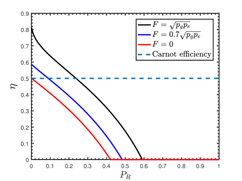
Figure 3: (color online) The efficiency $\eta$ with respect to the quantum probability $P_{R}$ of finding the system $S$ on the right side for different off-diagonal (coherent) element $F$. In the classical case, the efficiency must be limited by Carnot efficiency (the red line). However, with the coherence-assisted QMD, this limit may be allowed for a breakthrough (the case of pure sate with $F=\sqrt{p_{g}p_{e}}$ is depicted by black line and the blue line represents one of the mixed states with $F=0.7\sqrt{p_{g}p_{e}}$). Here we choose $T=1$, $T_{D}=0.5$, $\Delta=0.5$, and $F=F^{\ast}$.

Now turn to the crucial efficiency, which is defined as dividing the total work done by the system to the outside by total heat absorbed from the outside, namely

$$\eta=\frac{\langle W_{\text{tot}}\rangle}{\langle Q_{\text{tot}}\rangle}=1-\frac{P_{R}(p_{g}-p_{e})\Delta}{T(\Delta S_{\text{c}}+k_{\text{B}}\Delta C_{r})}.$$ (22)

Note that the coherence consumption appears in the denominator of the minuend, which implies the efficiency can be improved due to the coherence consumption of QMD. The more coherence consumed, the higher efficiency we can obtain. If there is no coherence being consumed, i.e. $\Delta C_{r}=0$, it will be limited by Carnot efficiency

$$\begin{split}\eta_{\max}&\geq\max\biggl{\{}\!1\!-\!\frac{P_{R}(p_{g}-p_{e})\Delta}{k_{\text{B}}T\Delta S_{\text{c}}}\biggr{\}}\\ &=\!\!\lim_{P_{R}\rightarrow 0}\!\textstyle\biggl{\{}\!1\!-\!\frac{(k_{\text{B}}T)^{-1}P_{R}(p_{g}-p_{e})\Delta}{p_{g}\ln{p_{g}}+p_{e}\ln{p_{e}}-{(p_{g}P_{L}\!+p_{e}P_{R})}\ln{(p_{g}P_{L}\!+p_{e}P_{R})}-{(p_{e}P_{L}\!+p_{g}P_{R})}\ln{(p_{e}P_{L}\!+p_{g}P_{R})}}\!\biggr{\}}\\ &=\!\!\lim_{P_{R}\rightarrow 0}\!\textstyle\biggl{\{}\!1\!-\!\frac{(k_{\text{B}}T)^{-1}P_{R}(p_{g}-p_{e})\Delta}{p_{g}\ln{p_{g}}+p_{e}\ln{p_{e}}-{(p_{g}P_{L})}\ln{(p_{g}P_{L})}-{(p_{e}P_{L})}\ln{(p_{e}P_{L})}+P_{R}(p_{g}-p_{e})\ln{(p_{g}/p_{e})})}\!\biggr{\}}\\ &=1-\frac{\Delta}{k_{\text{B}}T\ln{(p_{g}/p_{e})}}\\ &=1-\frac{T_{D}}{T},\end{split}$$ (23)

where the third line follows from the Taylor expansion $(c_{1}+c_{2}x)\ln{(c_{1}\!+\!c_{2}x)}\!=\!c_{1}\ln{c_{1}}+c_{2}(\ln{c_{1}}+1)x+o(x^{2})$ with $x\rightarrow 0$ (here $c_{1}$ and $c_{2}$ are constants), and the last line follows from the definition of $T_{D}:=\Delta/[k_{\text{B}}\ln{(p_{g}/p_{e})}]$ due to the initial probability distribution $p_{g}=1/(1+e^{-\beta_{D}\Delta})$ and $p_{e}=1-p_{g}$. This result speaks for itself, i.e., one may go beyond the classical Carnot efficiency $\eta_{\text{Carnot}}=1-T_{D}/T$ by consuming a certain amount of quantum coherence, see Fig. 3. But it is worth stressing that the quantum second law always holds though the classical Carnot bound can be violated, because the bound is defined by the diagonal elements. If we define the Carnot efficiency by considering both the diagonal and off-dagonal elements of QMD, then the total efficiency of the quantum thermodynamic cycle will be limited by this so-called quantum Carnot efficiency.

In particular, there exists a critical probability $P_{R}^{\text{cri}}$, below which the efficiency goes beyond the classical Carnot efficiency. According to Eq. (22), $P_{R}^{\text{cri}}$ satisfies $T_{D}(\Delta S_{\text{c}}+k_{\text{B}}\Delta C_{r})=P_{R}^{\text{cri}}(p_{g}-p_{e})\Delta$, which means QMD’s absorption of heat maintains balance with the energy flow of the total composite system. Furthermore, when $P_{R}$ is larger than a certain value $P_{R}^{0}$, the efficiency is zero. However, with the increase of coherence, the value of $P_{R}^{0}$ will become higher. This quirk is completely the quantum effect as it depends on how much resource of quantum coherence we expend, in the light of the quantitative resource theory of coherence.

5 Heat Engine Driven by Quantum Coherence and General Coherence-Modified Second Law

Additionally, we discuss an information heat engine (IHE) driven by quantum coherence, which is inspired by Ref. [58, 57]. The IHE is constituted by a system $S$ and a reservoir $R$, which is controlled by a demon consisting of two memories $A$ and $B$. One can extract work from this IHE by using quantum mutual information, or split into the classical correlation and quantum discord, between these two memories [58]. Then the IHE was generalized to multi-reservoirs case by Ren et al. who still discussed the work extractable in the same context of quantum discord [57]. Just according to the theme of the present work, a natural question is that whether work can be extracted from the inherent property of one quantum system—coherence, rather than the quantum correlation like discord between two or more systems. We replace the two memories with one memory $M$ in which quantum coherence exists but without any correlations, and investigate the relation between quantum coherence and work extractable from the engine. The schematic diagram of this coherent information heat engine is briefly shown in Fig. 4.

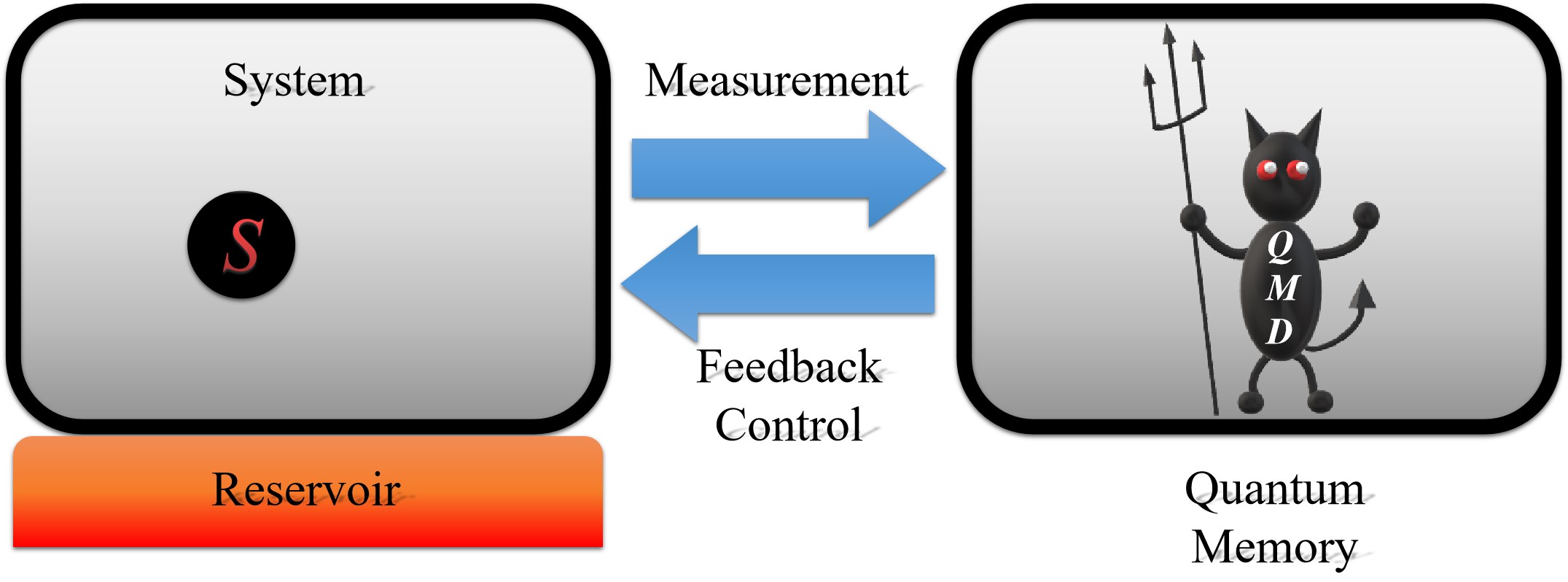
Figure 4: (color online) The schematic diagram of the information heat engine driven by quantum coherence.

Stage (i): Initial state.— Initially, the demon consisting of one memory $M$ is off-line and the system $S$ contacts with the reservoir $R$ at temperature $T=(k_{\text{B}}\beta)^{-1}$ in thermodynamic equilibrium, i.e. the total density matrix of the initial state is expressed as

$$\rho^{(i)}=\rho^{(i)}_{M}\otimes\rho^{(i)}_{SR}=\rho^{(i)}_{M}\otimes\frac{e^{-\beta H^{(i)}_{S}}}{Z^{(i)}_{S}}\otimes\frac{e^{-\beta H_{R}}}{Z_{R}},$$ (24)

where $Z^{(i)}_{S}=\mathrm{Tr}[e^{-\beta H^{(i)}_{S}}]$ and $Z_{R}=\mathrm{Tr}[e^{-\beta H_{R}}]$ are the initial partition functions of the system $S$ and the reservoir $R$, respectively. In general, there is no restriction on $\rho^{(i)}_{M}$.

Stage (ii): Unitary evolution.— The system $S$ begins to interact with $R$ (a unitary evolution), and $M$ is still off-line. Then the density matrix is given by

$$\rho^{(1)}=U^{(1)}\rho^{(i)}{U^{(1)}}^{\dagger},$$ (25)

with $U^{(1)}=I_{M}\otimes U^{(1)}_{SR}$. In this stage, the memory still doesn’t participate in the process of IHE.

Stage (iii): POVM.— This stage is where the demon consisting of $M$ started working. The measurement is performed by $M$ with POVMs (positive operator valued measures) [1, 25]. Explicitly, the measurement process is implemented by performing a unitary transformation $U^{(2)}$ on the whole system followed by a projection measurement $\{\Pi_{M}^{k}:|k\rangle_{M}\langle k|\}$ (a rank-1 projector) only on $M$, namley

$$\rho^{(2)}=\sum_{k}\Pi_{M}^{k}U^{(2)}\rho^{(1)}{U^{(2)}}^{\dagger}\Pi_{M}^{k}=\sum_{k}p_{k}|k\rangle_{M}\langle k|\otimes\rho_{SR}^{(2)k},$$ (26)

where $p_{k}=\mathrm{Tr}[\Pi_{M}^{k}U^{(2)}\rho^{(1)}{U^{(2)}}^{\dagger}\Pi_{M}^{k}]$ is the measurement outcome registered by the memory and the postmeasurement state of $SR$ is $\rho_{SR}^{(2)k}=\mathrm{Tr}_{A}[\Pi_{M}^{k}U^{(2)}\rho^{(1)}{U^{(2)}}^{\dagger}\Pi_{M}^{k}/p_{k}]$.

Stage (iv): Feedback control.— After measurement, the demon will control $SR$ according to the outcome $p_{k}$. Mathematically, this feedback control is performed by a unitary operator

$$U^{(3)}=\sum_{k}|k\rangle_{M}\langle k|\otimes U_{SR}^{k},$$ (27)

then the final state becomes

$$\rho^{(f)}=U^{(3)}\rho^{(2)}{U^{(3)}}^{\dagger}.$$ (28)

Note that the final state $\rho^{(f)}$ is not necessarily the canonical distribution, i.e. $\rho_{SR}^{(f)\text{can}}=\exp{(-\beta H_{S}^{(f)})}/Z_{S}^{(f)}\otimes\exp{(-\beta H_{R}})/Z_{R}$.

Since the POVMs increases the entropy while the unitary evolution ahead of the measurement keep it invariant, i.e., $S[\rho^{(2)}]\geq S[\rho^{(1)}]=S[U^{(1)}\rho^{(i)}{U^{(1)}}^{\dagger}]=S[\rho^{(i)}]$, one can obtain

$$S[\rho_{SR}^{(i)}]+S[\rho_{M}^{(i)}]\leq S[\rho_{M}^{(2)}]+\sum_{k}p_{k}S[\rho_{SR}^{(2)k}]\leq S[\rho_{M}^{(2)}]+S[\rho_{SR}^{(2)}],$$ (29)

where the second inequality follows from the subadditivity of von Neumann entropy [1].

Considering the final state of $SR$, i.e., $\rho_{SR}^{(f)}=\mathrm{Tr}_{M}[\rho^{(f)}]=\sum_{k}U_{SR}^{k}\rho_{SR}^{(2)k}U_{SR}^{k\dagger}$, we can obtain the following inequality by virtue of the concavity of the von Neumann entropy [1]

$$S[\rho_{SR}^{(f)}]\geq\sum_{k}p_{k}S[\rho_{SR}^{(2)k}].$$ (30)

Likewise, we have $\rho_{M}^{(f)}=\mathrm{Tr}_{SR}[\rho^{(f)}]=\sum_{k}|k\rangle_{M}\langle k|=\mathrm{Tr}_{SR}[\rho^{(2)}]=\rho_{M}^{(2)}$, thus

$$S[\rho_{M}^{(f)}]=S[\rho_{M}^{(2)}].$$ (31)

By substituting Eqs. (30) and (31) into Eq. (29), one obtains

$$S[\rho_{SR}^{(i)}]-S[\rho_{SR}^{(f)}]\leq S[\rho_{M}^{(f)}]-S[\rho_{M}^{(i)}],$$ (32)

which implies the entropy decrease of the heat engine and the reservoir cannot exceed the entropy increase of the memory, or should say, the whole system satisfies a general principle of entropy increase, i.e., $\Delta S_{SR}+\Delta S\geq 0$, where $\Delta S_{SR}=S[\rho_{SR}^{(f)}]-S[\rho_{SR}^{(i)}]$ and $\Delta S=S[\rho_{M}^{(f)}]-S[\rho_{M}^{(i)}]$. According to the quantum version of Klein’s inequality, i.e. $\mathrm{Tr}[\rho_{SR}^{(f)}\ln\rho_{SR}^{(f)\text{can}}]\leq\mathrm{Tr}[\rho_{SR}^{(f)}\ln\rho_{SR}^{(f)}]$ [25], Eq. (32) becomes

$$S[\rho_{SR}^{(i)}]+\mathrm{Tr}[\rho_{SR}^{(f)}\ln\rho_{SR}^{(f)\text{can}}]\leq\Delta S.$$ (33)

To investigate the work extractable from the heat engine, we turn the inequality above into the following form by using the canonical distributions $\rho_{SR}^{(i)}=\frac{e^{-\beta H^{(i)}_{S}}}{Z^{(i)}_{S}}\otimes\frac{e^{-\beta H_{R}}}{Z_{R}}$ and $\rho_{SR}^{(f)\text{can}}=\frac{e^{-\beta H^{(f)}_{S}}}{Z^{(f)}_{S}}\otimes\frac{e^{-\beta H_{R}}}{Z_{R}}$:

$$\langle E_{S}^{(i)}\rangle-\langle E_{S}^{(f)}\rangle+\langle E_{R}^{(i)}\rangle-\langle E_{R}^{(f)}\rangle\leq F_{S}^{(i)}-F_{S}^{(f)}+k_{\text{B}}T\Delta S$$ (34)

with $\langle E_{S}^{(i)}\rangle=\mathrm{Tr}[\rho_{S}^{(i)}H_{S}^{(i)}]$, $\langle E_{S}^{(f)}\rangle=\mathrm{Tr}[\rho_{S}^{(f)}H_{S}^{(f)}]$, $\langle E_{R}^{(i)}\rangle=\mathrm{Tr}[\rho_{R}^{(i)}H_{R}]$, $\langle E_{R}^{(f)}\rangle=\mathrm{Tr}[\rho_{R}^{(f)}H_{R}]$, $F_{S}^{(i)}=-k_{\text{B}}T\ln{Z_{S}^{(i)}}$, and $F_{S}^{(f)}=-k_{\text{B}}T\ln{Z_{S}^{(f)}}$. Here, the definition of the work extractable is $\langle W_{\text{ext}}\rangle:=-\langle\Delta E_{S}\rangle+\langle Q_{S}\rangle$, where $\langle\Delta E_{S}\rangle=\langle E_{S}^{(f)}\rangle-\langle E_{S}^{(i)}\rangle$ is the change of the internal energy of $S$ and $\langle Q_{S}\rangle=\langle E_{R}^{(f)}\rangle-\langle E_{R}^{(i)}\rangle$ is the heat exchange between $S$ and $R$, and thus we obtain

$$\langle W_{\text{ext}}\rangle\leq-\Delta F_{S}+T\Delta S_{\text{c}}+k_{\text{B}}T\Delta C_{r},$$ (35)

in which $\Delta F_{S}=F_{S}^{(f)}-F_{S}^{(i)}$ is the difference of free energy of the system, $\Delta S_{\text{c}}=k_{\text{B}}\Delta S_{\text{diag}}=k_{\text{B}}S[\rho_{M\text{diag}}^{(f)}]-k_{\text{B}}S[\rho_{M\text{diag}}^{(i)}]$ is the classical entropy change, $\Delta C_{r}=C_{r}[\rho_{M}^{(i)}]-C_{r}[\rho_{M}^{(f)}]$ is the coherence consumption of the memory. From Eq. (35), one can notice that if the contribution of $\Delta F_{S}$ is ignored, the bound of the work extractable is given by the total entropy change of the memory, which is split into the change of incoherent part and coherence consumption. Even if no classical entropy changes, i.e. $\Delta S_{\text{c}}=0$, we still find the maximum work extractable is given by coherence consumption, namely

$$\langle W_{\text{ext}}\rangle\leq k_{\text{B}}T\Delta C_{r},$$ (36)

which is also in support of the resource-driven viewpoint, specifically, one can extract work from quantum coherence, a potential quantum physical resource, to drive a heat engine.

6 Extending to More General Thermodynamics involving Quantum Coherence

We consider a general quantum system described as $H|\psi_{n}\rangle=E_{n}|\psi_{n}\rangle$, where $H$, $E_{n}$ and $|\psi_{n}\rangle$ are the Hamiltonian, $n$-th eigenenergy and eigenstate, respectively. Here, the system is not necessarily to be a single system. It might be composed of multiple subsystems. In the energy representation, a general density matrix of this system can be given by

$$\rho=\sum_{n}P_{n}|\psi_{n}\rangle\langle\psi_{n}|+\sum_{n\neq m}P_{nm}|\psi_{n}\rangle\langle\psi_{m}|,$$ (37)

then the internal energy of the system can be expressed as

$$\langle E\rangle=\mathrm{Tr}[\rho H]=\sum_{n}P_{n}E_{n}$$ (38)

where $P_{n}$ is the probability distribution of $n$-th energy eigenstate. In equilibrium $P_{n}$ obeys the canonical distribution. Note that although the density matrix contains off-diagonal part, the internal energy of the system is only connected with the diagonal part due to the energy representation.

From the derivative of $\langle E\rangle$, one obtains $\mathrm{d}\langle E\rangle=\sum_{n}(E_{n}\mathrm{d}P_{n}+P_{n}\mathrm{d}E_{n})$. Here, the previous viewpoint is analogizing it to the classical thermodynamic first law, i.e., $\mathrm{d}W_{\text{c}}=-\mathrm{d}E_{\text{c}}+\mathrm{d}Q_{\text{c}}=-\mathrm{d}E_{\text{c}}+T\mathrm{d}S_{\text{c}}$, where $E_{\text{c}}$, $W_{\text{c}}$, $Q_{\text{c}}$ and $S_{\text{c}}$ are the classical internal energy, work, heat and entropy, respectively. Then, the quantum work can be identified as $\mathrm{d}\langle W\rangle=-\sum_{n}P_{n}\mathrm{d}E_{n}$ [41, 42, 43], and quantum heat is $\mathrm{d}\langle Q\rangle=\sum_{n}E_{n}\mathrm{d}P_{n}$ associated with $T\mathrm{d}S_{\text{c}}$ since the classical entropy $S_{\text{c}}$ is defined as $S_{\text{c}}=-k_{\text{B}}\sum_{n}P_{n}\ln{P_{n}}$.

Nevertheless, one has already noticed that the classical entropy is actually the von Neumann entropy of diagonal density matrix in energy representation, namely

$$S_{\text{c}}=k_{\text{B}}S(\rho_{\text{diag}}),$$ (39)

where $k_{\text{B}}$ is the Boltzmanns constant and $\rho_{\text{diag}}=\sum_{n}\langle\psi_{n}|\rho|\psi_{n}\rangle|\psi_{n}\rangle\langle\psi_{n}|$ denotes the diagonal part of $\rho$. Therefore, with the analogy above, this quantum system must have lost part of the information concerning its non-equilibrium (off-diagonal) state. To describe the whole quantum state, the entropy must be the whole $k_{\text{B}}S(\rho)$ instead of $k_{\text{B}}S(\rho_{\text{diag}})$ which contains only the information of equilibrium (diagonal). Hence, combined with Eq. (1), it is natural to define the quantum heat as

$$\langle Q\rangle=\int\limits_{\rho\rightarrow\sigma}\sum_{n}E_{n}\mathrm{d}P_{n}+k_{\text{B}}T\Delta C_{r},$$ (40)

where $\Delta C_{r}=C_{r}(\rho)-C_{r}(\sigma)$ is the coherence consumption of the system from the initial state $\rho$ to the final state $\sigma$. Then the first term of the right-hand side of Eq. (40) only determined by the diagonal (incoherent) part $P_{n}$ can be considered as the incoherent heat, i.e., $\langle Q_{\text{incoh}}\rangle=\int_{\rho\rightarrow\sigma}\sum_{n}E_{n}\mathrm{d}P_{n}=TS_{\text{c}}=k_{\text{B}}TS(\rho_{\text{diag}})$, and the second term can be understood as the coherent heat, i.e., $\langle Q_{\text{coh}}\rangle=k_{\text{B}}T\Delta C_{r}$. Thus,

$$\langle Q\rangle=\langle Q_{\text{incoh}}\rangle+\langle Q_{\text{coh}}\rangle,$$ (41)

which gives the physical origin of quantum heat: the change of diagonal (incoherent) distribution and the coherence consumption.

By virtue of the definition of quantum heat in Eq. (40), we can define the quantum work as

$$\langle W\rangle=-\int\limits_{\rho\rightarrow\sigma}\sum_{n}P_{n}\mathrm{d}E_{n}+k_{\text{B}}T\Delta C_{r},$$ (42)

since the first law $\langle\Delta E\rangle=-\langle W\rangle+\langle Q\rangle$. Likewise, the quantum work can be written as

$$\langle W\rangle=\langle W_{\text{incoh}}\rangle+\langle W_{\text{coh}}\rangle,$$ (43)

with the incoherent work $\langle W_{\text{incoh}}\rangle=-\int_{\rho\rightarrow\sigma}\sum_{n}P_{n}\mathrm{d}E_{n}$ and the coherent work $\langle W_{\text{coh}}\rangle=k_{\text{B}}T\Delta C_{r}$. So the quantum work can be viewed as the contribution of both the change of energy level under the invariable diagonal (incoherent) distribution and the coherence consumption.

In this way, the total internal energy don’t concern the off-diagonal part. However, because the total work can be enhanced due to the coherent superposition, the efficiency of a quantum heat engine thus can be improved in the thermodynamic process involving quantum coherence.

7 Conclusions

In summary, we propose and study quantum thermodynamics by utilizing the resource theory of coherence. Two kinds of quantum heat engine assisted by a coherent QMD are discussed in details, which are based on QSE and IHE, respectively. The quantum thermodynamic cycle based on QSE is divided into five stages: initial state, insertion, measurement, expansion and removal, which are all described by the evolution of quantum ensembles. We explicitly calculated the total quantum work, heat and the corresponding efficiency of this thermodynamic cycle. From a resource-driven viewpoint, the efficiency can be enhanced due to the coherence consumption of QMD, which is one of our main results.

In addition, we discuss an universal engine driven by quantum coherence based on IHE, which is also to achieve the whole measurement and feedback control through QMD. The maximum work extractable is given by the consumption of quantum coherence, leading to a coherence-modified second law. Consequently, one can extract work from quantum coherence to drive this heat engine even without any classical resources.

Finally, the subtle connection between coherence and fundamental thermodynamic notions is extended to a more general quantum thermodynamics. The quantum work and heat can be naturally redefined as a sum of incoherent and coherent parts by considering the first and second thermodynamic laws. Our results are enlighten for the quantum information processes in thermodynamic systems where the coherent superposition of states cannot be ignored.

References

References

- [1] Nielsen M A and Chuang I L 2000 Quantum Computation and Quantum Information (Cambridge University Press, Cambridge)
- [2] Vedral V 2002 The role of relative entropy in quantum information theory Rev. Mod. Phys. 74 197
- [3] Parrondo J M R, Horowitz J M and Sagawa T 2015 Thermodynamics of information Nat. Phys. 11 131-139
- [4] Goold J, Huber M, Riera A, del Rio L and Skrzypczyk P 2016 The role of quantum information in thermodynamics–a topical review J. Phys. A 49 143001
- [5] Binder F, Vinjanampathy S, Modi K and Goold J 2015 Quantum thermodynamics of general quantum processes Phys. Rev. E 91 032119
- [6] Strasberg P, Schaller G, Brandes T and Esposito M 2017 Quantum and Information Thermodynamics: A Unifying Framework Based on Repeated Interactions Phys. Rev. X 7 021003
- [7] Horodecki M and Oppenheim J 2013 Fundamental limitations for quantum and nanoscale thermodynamics Nat. Commun. 4 2059
- [8] Brando F, Horodecki M, Ng N, Oppenheim J and Wehner S 2015 The second laws of quantum thermodynamics PNAS 112 3275-3279
- [9] wikliski P, Studziski M, Horodecki M and Oppenheim J 2015 Limitations on the Evolution of Quantum Coherences: Towards Fully Quantum Second Laws of Thermodynamics Phys. Rev. Lett. 115 210403
- [10] Alhambra M, Wehner S, Wilde M M and Woods M P 2018 Work and reversibility in quantum thermodynamics Phys. Rev. A 97 062114
- [11] Francica G, Goold J and Plastina F 2019 The role of coherence in the non-equilibrium thermodynamics of quantum systems Phys. Rev. E 99 042105
- [12] Santos J P, Cleri L C, Landi G T and Paternostro M 2017 The role of quantum coherence in non-equilibrium entropy production (arXiv:1707.08946)
- [13] Baumgratz T, Cramer M and Plenio M B 2014 Quantifying Coherence Phys. Rev. Lett. 113 140401
- [14] Streltsov A, Adesso G and Plenio M B 2017 Colloquium: Quantum Coherence as a Resource Rev. Mod. Phys. 89 041003
- [15] Hu M-L, Hu X, Wang J, Peng Y, Zhang Y-R and Fan H 2018 Quantum coherence and geometric quantum discord Phys. Rep. 762 1
- [16] Winter A and Yang D 2016 Operational Resource Theory of Coherence Phys. Rev. Lett. 116 120404
- [17] Vedral V, Plenio M B, Rippin M A and Knight P L 1997 Quantifying Entanglement Phys. Rev. Lett. 78 2275
- [18] Ollivier H and Zurek W H 2001 Quantum Discord: A Measure of the Quantumness of Correlations Phys. Rev. Lett. 88 017901
- [19] Jarzynski C 1997 Nonequilibrium Equality for Free Energy Differences Phys. Rev. Lett. 78 2690
- [20] Tasaki H 2000 Jarzynski Relations for Quantum Systems and Some Applications (arXiv: cond-mat/0009244)
- [21] Campisi M, Hnggi P and Talkner P 2011 Colloquium: Quantum fluctuation relations: Foundations and applications Rev. Mod. Phys. 83 771
- [22] Potts P P and Samuelsson P 2018 Detailed Fluctuation Relation for Arbitrary Measurement and Feedback Schemes Phys. Rev. Lett. 121 210603
- [23] Iyoda E, Kaneko K and Sagawa T 2017 Fluctuation Theorem for Many-Body Pure Quantum States Phys. Rev. Lett. 119 100601
- [24] Park J J, Kim S W and Vedral V 2017 Fluctuation Theorem for Arbitrary Quantum Bipartite Systems (arXiv:1705.01750)
- [25] Sagawa T 2013 Thermodynamics of Information Processing in Small Systems (Springer)
- [26] Mandal D, Quan H T and Jarzynski C 2013 Maxwell’s Refrigerator: An Exactly Solvable Model Phys. Rev. Lett. 111 030602
- [27] Mancino L, Cavina V, DePasquale A, Sbroscia M, Booth R I, Roccia E, Gianani I, Giovannetti V and Barbieri M 2018 Geometrical Bounds on Irreversibility in Open Quantum Systems Phys. Rev. Lett. 121 160602
- [28] Maxwell J C 1871 Theory of Heat (Longmans, London)
- [29] Szilard L 1929 ber die Entropieverminderung in einem thermodynamischen System bei Eingriffen intelligenter Wesen Z. Phys. 53 840
- [30] Maruyama K, Nori F and Vedral V 2009 Colloquium: The physics of Maxwell’s demon and information Rev. Mod. Phys. 81 1
- [31] Campisi M, Pekola J and Fazio R 2017 Feedback-controlled heat transport in quantum devices: theory and solid-state experimental proposal New. J. Phys. 19 053027
- [32] Cherubim C, Brito F, and Deffner S 2019 Non-thermal quantum engine in transmon qubits Entropy 21 545
- [33] Salamon P, Hoffmann K H, Rezek Y, and Kosloff R 2009 Maximum work in minimum time from a conservative quantum system Phys. Chem. Chem. Phys. 11 1027-1032
- [34] Stefanatos D 2017 Minimum-time transitions between thermal equilibrium states of the quantum parametric oscillator IEEE Trans. Automat. Control 62 pp. 4290-4297
- [35] Buffoni L, Solfanelli A, Verrucchi P, Cuccoli A, and Campisi M 2019 Quantum Measurement Cooling Phys. Rev. Lett. 122 070603
- [36] Landauer R 1961 Irreversibility and heat generation in the computing process IBM J. Res. Dev. 5 183
- [37] Brut A, Arakelyan A, Petrosyan A, Ciliberto S, Dillenschneider R and Lutz E 2012 Experimental verification of Landauer s principle linking information and thermodynamics Nature (London) 483 187
- [38] Vedral V 2012 Using Temporal Entanglement to Perform Thermodynamical Work (arXiv:1204.5559)
- [39] Funo K and Quan H T 2018 Path Integral Approach to Quantum Thermodynamics Phys. Rev. Lett. 121 040602
- [40] Kurchan J 2001 A Quantum Fluctuation Theorem (arXiv:cond-mat/0007360)
- [41] Kieu T D 2004 The Second Law, Maxwell’s Demon, and Work Derivable from Quantum Heat Engines Phys. Rev. Lett. 93 140403
- [42] Esposito M and Mukamel S 2006 Fluctuation theorems for quantum master equations Phys. Rev. E 73 046129
- [43] Kim S W, Sagawa T, DeLiberato S and Ueda M 2011 Quantum Szilard Engine Phys. Rev. Lett. 106 070401
- [44] Plesch M, Dahlsten O, Goold J and Vedral V 2013 Comment on Quantum Szilard Engine Phys. Rev. Lett. 111 188901
- [45] Shi H-L, Liu S-Y, Wang X-H, Yang W-L, Yang Z-Y and Fan H 2017 Coherence depletion in the Grover quantum search algorithm Phys. Rev. A 95 032307
- [46] Misra A, Singh U, Bhattacharya S and Pati A K 2016 Energy cost of creating quantum coherence Phys. Rev. A 93 052335
- [47] Zurek W H 2003 Quantum discord and Maxwell’s demons Phys. Rev. A 67 012320
- [48] Quan H T, Wang Y D, Liu Y-X, Sun C P and Nori F 2006 Maxwell’s Demon Assisted Thermodynamic Cycle in Superconducting Quantum Circuits Phys. Rev. Lett. 97 180402
- [49] Dong H, Xu D Z, Cai C Y and Sun C P 2011 Quantum Maxwell’s demon in thermodynamic cycles Phys. Rev. E 83 061108
- [50] Naghiloo M, Alonso J J, Romito A, Lutz E and Murch K W 2018 Information Gain and Loss for a Quantum Maxwell’s Demon Phys. Rev. Lett. 121 030604
- [51] Elouard C, Herrera-Marti D, Huard B and Auffves A 2017 Extracting Work from Quantum Measurement in Maxwell’s Demon Engines Phys. Rev. Lett. 118 260603
- [52] Camati P A, Peterson J P S, Batalho T B, Micadei K, Souza A M, Sarthour R S, Oliveira I S and Serra R M 2016 Experimental Rectification of Entropy Production by Maxwell’s Demon in a Quantum System Phys. Rev. Lett. 117 240502
- [53] Vidrighin M D, Dahlsten O, Barbieri M, Kim M S, Vedral V and Walmsley I A 2016 Photonic Maxwell’s Demon Phys. Rev. Lett. 116 050401
- [54] Koski J V, Kutvonen A, Khaymovich I M, Ala-Nissila T and Pekola J P 2015 On-Chip Maxwell’s Demon as an Information-Powered Refrigerator Phys. Rev. Lett. 115 260602
- [55] Koski J V, Maisi V F, Sagawa T and Pekola J P 2014 Experimental Observation of the Role of Mutual Information in the Nonequilibrium Dynamics of a Maxwell Demon Phys. Rev. Lett. 113 030601
- [56] Toyabe S, Sagawa T, Ueda M, Muneyuki E and Sano M 2010 Experimental demonstration of information-to-energy conversion and validation of the generalized Jarzynski equality Nat. Phys. 6 819-832
- [57] Ren L-H and Fan H 2017 Second law of thermodynamics with quantum memory Phys. Rev. A 96 042304
- [58] Park, J J, Kim K-H, Sagawa T and Kim S W 2013 Heat Engine Driven by Purely Quantum Information Phys. Rev. Lett. 111 230402
- [59] Sagawa T and Ueda M 2008 Second Law of Thermodynamics with Discrete Quantum Feedback Control. Phys. Rev. Lett. 100, 080403
- [60] Sagawa T and Ueda M 2009 Minimal Energy Cost for Thermodynamic Information Processing: Measurement and Information Erasure Phys. Rev. Lett. 102 250602