Time fractals and discrete scale invariance with trapped ions

Abstract

We show that a one-dimensional chain of trapped ions can be engineered to produce a quantum mechanical system with discrete scale invariance and fractal-like time dependence. By discrete scale invariance we mean a system that replicates itself under a rescaling of distance for some scale factor, and a time fractal is a signal that is invariant under the rescaling of time. These features are reminiscent of the Efimov effect, which has been predicted and observed in bound states of three-body systems. We demonstrate that discrete scale invariance in the trapped ion system can be controlled with two independently tunable parameters. We also discuss the extension to $n$-body states where the discrete scaling symmetry has an exotic heterogeneous structure. The results we present can be realized using currently available technologies developed for trapped ion quantum systems.

In this work we show how to construct a one-dimensional system of trapped ions with discrete scale invariance and fractal-like time dependence. In classical systems scale invariance arises when the scale transformation acting on spatial coordinates, $r\rightarrow\lambda r,$ is a symmetry of the dynamics. This arises naturally if the Hamiltonian transforms homogeneously under rescaling. When the Hamiltonian is quantized, however, this scale invariance cannot persist for bound state solutions with discrete energy levels. Instead, the scale invariance is broken through a quantum scale anomaly. An analogous effect occurs in relativistic field theories and is responsible for the mass gap in the spectrum of non-Abelian gauge theories such as quantum chromodynamics.

While the quantum scale anomaly spoils invariance under a general scale transformation, it may preserve the symmetry associated with a discrete set of scale transformations. This was first described by Efimov for the bound state spectrum of three bosons with short-range interactions tuned to infinite scattering length Efimov (1971, 1993); Bedaque et al. (1999a, b). See also Ref. Coon and Holstein (2002) for a review of anomalies in quantum mechanics and the attractive $1/r^{2}$ potential. Efimov trimers were first observed experimentally through the loss rate of trapped ultracold cesium atoms Kraemer et al. (2006), and a more direct observation has been made using the Coulomb explosion of helium trimers Kunitski et al. (2015). As the underlying physics is of universal character, the application and generalization of the Efimov effect has been considered in various settings, including nuclear physics Bedaque et al. (2000); Hagen et al. (2013), bound states with more than three particles Platter et al. (2004); Hammer and Platter (2007); von Stecher et al. (2009); von Stecher (2011); Carlson et al. (2017), systems with reduced dimensions Nishida and Tan (2011); Moroz et al. (2013); Happ et al. (2019), quantum magnets Nishida et al. (2013), molecules with spatially-varying interactions Nishida and Lee (2012), and Dirac fermions in graphene Ovdat et al. (2017).

We demonstrate that quantum scale anomalies can be produced with trapped ion quantum systems. We start with a one-dimensional chain of ions in a radio-frequency trap with qubits represented by two hyperfine “clock” states. Such systems have been investigated by the trapped ion group at the University of Maryland using ¹⁷¹Yb⁺ ions Zhang et al. (2017a, b). Similar efforts have been pioneered by trapped ion groups at ETH Zürich, Freiburg, Innsbruck, Mainz, Stockholm, and the Weizmann Institute. Off-resonant laser beams are used to drive stimulated Raman transitions for all ions in the trap. This induces effective interactions between all qubits with a power-law dependence on separation distance. We define the vacuum state as the state with $\sigma^{z}_{i}=1$ for all $i$. We use interactions of the form $\sigma^{x}_{i}\sigma^{x}_{j}+\sigma^{y}_{i}\sigma^{y}_{j}$, to achieve the hopping of spin excitations. We then use a $\sigma^{z}_{i}\sigma^{z}_{j}$ interaction to produce a two-body potential felt by pairs of spin excitations, and we also consider an external one-body potential coupled to $\sigma^{z}_{i}$.

We can view each spin excitation with $\sigma^{z}_{i}=-1$ as a bosonic particle at site $i$ with hardcore interactions preventing multiple occupancy. In this language, the Hamiltonian we consider has the form

$$H=\frac{1}{2}\sum_{i}\sum_{j\neq i}J_{ij}[b^{\dagger}_{i}b_{j}+b^{\dagger}_{j}b_{i}] +\frac{1}{2}\sum_{i}\sum_{j\neq i}V_{ij}b^{\dagger}_{i}b_{i}b^{\dagger}_{j}b_{j}$$

$$+\sum_{i}U_{i}b^{\dagger}_{i}b_{i}+C,$$ (1)

where $b_{i}$ and $b^{\dagger}_{i}$ are annihilation and creation operators for the hardcore bosons on site $i$. See the Supplemental Materials for a derivation of this Hamiltonian. The parameter $C$ is just an overall energy constant. The hopping coefficients $J_{ij}$ have the asymptotic form $J_{ij}=J_{0}/|r_{i}-r_{j}|^{\alpha}$, where $r_{i}$ is the position of qubit $i$. For the purposes of this study, we assume $J_{ij}$ to have exactly this form for $i\neq j.$ Similarly, the two-body potential coefficients $V_{ij}$ have the asymptotic form $V_{ij}=V_{0}/|r_{i}-r_{j}|^{\beta}$. In this work we assume $V_{ij}$ to have exactly this form for $i\neq j$. We consider the case where the lattice of ions is uniform and large, and we start with a constant potential $U_{i}$ chosen so that bosons with zero momentum have zero energy. Both positive (anti-ferromagnetic) and negative (ferromagnetic) values can be realized for $J_{0}$ and $V_{0}$. The exponents $\alpha$ and $\beta$ can in principle vary in the range between $0$ and $3$. However, in practice the range between $0.5$ and $1.8$ is favored in order to enhance coherence times and reduce experimental drifts Zhang et al. (2017b).

We now add to $U_{i}$ a deep attractive potential at some chosen site $i_{0}$ that traps and immobilizes one boson at that site. Without loss of generality, we take the position of that site to be the origin and add a constant to the Hamiltonian so that the energy of the trapped boson is zero. We then consider the dynamics of a second boson that feels the interactions with this fixed boson at the origin. In order to produce a Hamiltonian with classical scale invariance, we choose $\beta=\alpha-1$. Then at low energies, our low-energy Hamiltonian for the second boson has the form

$$H(p,r)=2J_{0}\sin(\alpha\pi/2)\Gamma(1-\alpha)|p|^{\alpha-1}+\frac{V_{0}}{|r|^{\alpha-1}},$$ (2)

where we omit corrections of size $O(p^{2})$. We are interested in the case where both $J_{0}$ and $V_{0}$ are negative. In that case we find an infinite tower of even parity and odd parity bound states. We label the bound state energies as $E^{(n)}_{+}$ and $E^{(n)}_{-}$, respectively, for nonnegative integers $n$. As expected, our quantized system has a quantum scale anomaly and we are left with two discrete scale symmetries, $r\rightarrow\lambda_{+}r$ for even parity and $r\rightarrow\lambda_{-}r$ for odd parity. Correspondingly, the bound state energies follow a simple geometrical progression, $E^{(n)}_{+}=E^{(0)}_{+}\lambda_{+}^{-n}$ and $E^{(n)}_{-}=E^{(0)}_{-}\lambda_{-}^{-n}$. In the Supplemental Materials we provide details of the discrete scale invariance for general $\alpha$. For the special case $\alpha=2$, the scale factors are $\lambda_{\pm}=\exp(\pi/\delta_{\pm}),$ where

$$\delta_{+}=\frac{V_{0}}{J_{0}\pi}\coth(\delta_{+}\pi/2),\;\;\delta_{-}=\frac{V_{0}}{J_{0}\pi}\tanh(\delta_{-}\pi/2).$$ (3)

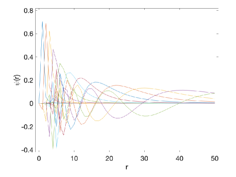
Figure 1: Bound state wave functions. Plot of the normalized wave functions for the first twelve even-parity bound states for the case $\alpha=2$, $\beta=1$, $J_{0}=-1$, and $V_{0}=-30$. We plot the region $r>0$. All quantities are in dimensionless lattice units.

In contrast with most other systems with a quantum scale anomaly, we note that the properties of our ion trap system can be tuned using two different adjustable parameters, $V_{0}/J_{0}$ and $\alpha$. This is convenient for probing a wide range of different phenomena exhibiting discrete scaling symmetry. In the following we will work in lattice units where physical quantities are multiplied by powers of the lattice spacing to make the combination dimensionless and have set $\hbar=1$. As an example, consider a system with $\alpha=2$, $\beta=1$, $J_{0}=-1$, and $V_{0}=-30$. The wave functions for the first twelve even-parity bound states are shown in Fig. 1. We plot the normalized wave function for $r>0$. We see clear evidence of discrete scale invariance emerging as we approach zero energy. In Table 1 we show the energies for the first fourteen even-parity and odd-parity bound states and the ratios between consecutive energies. For comparison, at the bottom we show the predictions for these ratios as we approach zero energy at infinite volume. We see that the agreement is quite good.

$n$	$E^{(n)}_{+}$	$E^{(n-1)}_{+}/E^{(n)}_{+}$	$E^{(n)}_{-}$	$E^{(n-1)}_{-}/E^{(n)}_{+}$
$0$	$-27.05304149$	$-$	$-26.5188669$	$-$
$1$	$-11.93067205$	$2.267520336$	$-11.79861873$	$2.247624701$
$2$	$-6.977774689$	$1.709810446$	$-6.919891389$	$1.705029468$
$3$	$-4.553270276$	$1.5324754$	$-4.521425357$	$1.530466798$
$4$	$-3.139972298$	$1.450098869$	$-3.120231851$	$1.449067112$
$5$	$-2.233327278$	$1.405961557$	$-2.220194049$	$1.405386998$
$6$	$-1.617052389$	$1.381110033$	$-1.607920414$	$1.380786033$
$7$	$-1.182654461$	$1.367307563$	$-1.176124883$	$1.367134084$
$8$	$-0.869406941$	$1.360300229$	$-0.864656962$	$1.360221377$
$9$	$-0.640405903$	$1.357587332$	$-0.636916042$	$1.357568195$
$10$	$-0.471738446$	$1.357544438$	$-0.469161911$	$1.357561276$
$11$	$-0.347112043$	$1.359037968$	$-0.345207121$	$1.359073675$
$12$	$-0.254996818$	$1.361240684$	$-0.253589633$	$1.361282464$
$13$	$-0.187011843$	$1.363532996$	$-0.18597462$	$1.363571189$
theory	–	$\lambda_{+}=1.3895595319$	–	$\lambda_{-}=1.3895595319$

Table 1: Bound state energies. Energies for the first fourteen even-parity and odd-parity bound states and ratios between consecutive energies for the case $\alpha=2$, $\beta=1$, $J_{0}=-1$, and $V_{0}=-30$. For comparison we show the theoretical predictions for the ratios $\lambda_{+}$ and $\lambda_{-}$ as we approach zero energy at infinite volume.

One intriguing question is how discrete scale invariance could persist in quantum many-body systems. It has been demonstrated numerically that the Efimov effect extends beyond bosonic trimers and describes the properties of $n$-boson systems with the same discrete scaling factor Platter et al. (2004); Hammer and Platter (2007); von Stecher et al. (2009); von Stecher (2011); Carlson et al. (2017) . As we will see, something quite different happens in the trapped ion system. Let us start from a particular bound state of the two-body system and ask what happens when we introduce a third boson that is weakly bound and very far from the origin. The effective Hamiltonian for the third boson contains a potential energy that is doubled due to interactions of the weakly-bound third boson with the two other bosons. As a result of the stronger attractive interaction, the geometric scaling factors $\lambda_{\pm}$ for the third boson will be smaller than for the two-body system. This argument can be generalized to describe weakly-bound states for the general $n$-body system. The effective potential for the $n^{\rm th}$ boson will be a factor of $n-1$ times larger, and thus the scaling of the $n$-body energies relative to each $(n-1)$-body threshold is different from the scaling of the $k$-body bound states for each $k$ between $1$ and $n$. The properties of these exotic systems with heterogeneous discrete invariance will be investigated further in future work.

Let us now consider an initial state $|S\rangle=\sum_{n=0}^{N-1}|\psi^{(n)}_{+}\rangle,$ where we sum over the first $N$ even-parity two-boson bound states $|\psi^{(n)}_{+}\rangle$ with equal weight. We choose the even-parity states, but we could just as easily choose odd-parity states. The phase convention for each $|\psi^{(n)}_{+}\rangle$ is chosen so that the tail of the wave function is real and positive at large $r$. We note that the time dependent amplitude $A(t)={\rm Re}[\langle S|\exp(-iHt)|S\rangle]$ is invariant under the rescaling $t\rightarrow\lambda^{\alpha-1}_{+}t$, thus endowing it with the properties of a time fractal.  The time fractal is particularly interesting for the case when $\lambda^{\alpha-1}_{+}$ is an integer so that each of the higher frequencies in $A(t)$ are integer multiples of the lower frequencies.

For the case $\alpha=2$ and $J_{0}=-1$, we can produce the time scaling factor $\lambda^{\alpha-1}_{+}=\lambda_{+}=2$ by setting $V_{0}=-14.2388293$. In Fig. 2 we show the amplitude $A(t)$ ranging from $t=0$ to $80$ in the upper left, $t=0$ to $160$ in the upper right, $t=0$ to $320$ in the lower left, and $t=0$ to $640$ in the lower right. Aside from small deviations, we see that the time dependence shows fractal-like self-similarity when we zoom in or out by a scale factor very close to $2$. The best fit for the scale factor is approximately $1.9$. In the Supplemental Materials we show how a time fractal can be realized experimentally using quantum interference on a trapped ion quantum system.

The time fractals that we have discussed are closely related to the Weierstrass function $w(x)=\sum_{n=0}^{\infty}a^{n}\cos(b^{n}\pi x)$. Weierstrass showed that this function is continuous everywhere but differentiable nowhere when $0<a<1$, $b$ is an odd integer, and $ab>1+3\pi/2$ Weierstrass (1886). Hardy extended the proof to any $0<a<1<b$ and $ab\geq 1$  Hardy (1916). We note that $aw(bx)$ equals $w(x)$ plus the smooth function $\cos(\pi x)$, and this suggests that the fractal dimension of the Weierstrass function should given by Hunt (1998)

$$D=2+\frac{\log a}{\log b}.$$ (4)

This result for the fractal dimension is confirmed by the box-counting method for determining fractal dimensions Kaplan et al. (1984).

Our initial state $|S\rangle=\sum_{n=0}^{N-1}|\psi^{(n)}_{+}\rangle$ produces the fractal-like amplitude

$$A(t)=\sum_{n=0}^{N-1}\cos(E^{(n)}_{+}t)=\sum_{n=0}^{N-1}\cos(\epsilon_{+}\lambda_{+}^{-n}t).$$ (5)

In the limit of large $N$, our choice of parameters corresponds to the limiting case $a\rightarrow 1$ and $b=\lambda_{+}$, with $x=\epsilon_{+}\lambda_{+}^{-N+1}t/{\pi}$. Therefore, the fractal dimension for our time fractal will be $D=2$. If we instead choose the initial state to have the form $|S(a)\rangle=\sum_{n=0}^{N-1}a^{n/2}|\psi^{(n)}_{+}\rangle$ for $a<1,$ then in the limit $N\rightarrow\infty$, the fractal dimension will be

$$D=2+\frac{\log a}{\log\lambda_{+}}.$$ (6)

There are many interesting related phenomena that one can explore in connection with time fractals and the dynamics of systems with discrete scale invariance. One fascinating topic is the adiabatic evolution of a system with discrete invariance as the interactions are varied slowly. Another is the response of a system with discrete scale invariance when driven in resonance with one of its bound state energies. In this letter we have shown that the intrinsic power-law interactions of the trapped ion system make it an ideal system for exploring the physics of quantum scale anomalies, discrete scale invariance, and time fractals. There are clearly many directions that one can explore in this new area, and we look forward to working with others to develop further applications and experimental realizations of many of these concepts.

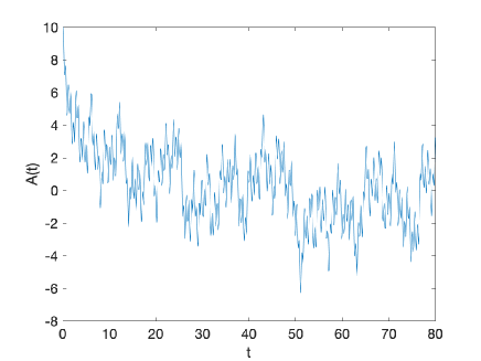
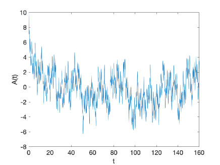
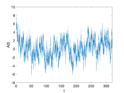
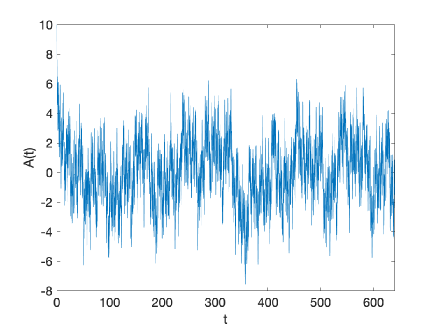
Figure 2: Time fractals. The amplitude $A(t)$ is displayed over the range from $t=0$ to $80$ in the upper left, $t=0$ to $160$ in the upper right, $t=0$ to $320$ in the lower left, and $t=0$ to $640$ in the lower right. All quantities are in dimensionless lattice units.

We are grateful for discussions with Zohreh Davoudi, Chao Gao, Pavel Lougovski, Titus Morris, Thomas Papenbrock, and Raphael Pooser. We acknowledge financial support from the U.S. Department of Energy (DE-SC0018638 and DE-AC52-06NA25396). Computational resources were provided by the Julich Supercomputing Centre at Forschungszentrum Jülich, Oak Ridge Leadership Computing Facility, RWTH Aachen, and Michigan State University.

I Supplemental Material

Trapped ion Hamiltonian

For our one-dimensional trapped ion system, the Hamiltonian we consider is

$$H=T+V_{2}+U+C,$$ (7)

where

$$T =\frac{1}{4}\sum_{i}\sum_{j\neq i}J_{ij}(\sigma^{x}_{i}\sigma^{x}_{j}+\sigma^{y}_{i}\sigma^{y}_{j}),$$ (8)

$$V_{2} =\frac{1}{8}\sum_{i}\sum_{j\neq i}V_{ij}(1-\sigma^{z}_{i})(1-\sigma^{z}_{j}),$$ (9)

$$U =\frac{1}{2}\sum_{i}U_{i}(1-\sigma^{z}_{i}),$$ (10)

and $C$ is a constant. We regard each spin configuration with $\sigma^{z}=-1$ as a particle excitation. Thus $T$ corresponds to the hopping of a single particle, $V_{2}$ is a two-particle interaction, and $U$ is a one-particle potential. In Fig. S1 we show a sketch of the action of the hopping coefficient $J_{ij}$. In Fig. S2 we show a sketch of the two-body interaction potential $V_{ij}$. Without loss of generality, we assume that both $J_{ij}$ and $V_{ij}$ are symmetric in the indices $i,j.$

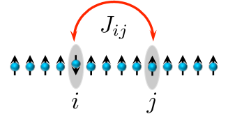
Figure S1: Hopping coefficient $J_{ij}$. This sketch shows the action of the hopping coefficient $J_{ij}$ for a single particle between sites $i$ and $j$. Particle excitations correspond with sites where $\sigma^{z}=-1$.

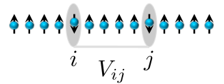
Figure S2: Interaction potential $V_{ij}$. This sketch shows the two-body interaction potential $V_{ij}$ between two particles at sites $i$ and $j$. Particle excitations correspond with sites where $\sigma^{z}=-1.$

We can reorganize the $\sigma^{z}$ terms as

$$V_{2}+U=\frac{1}{8}\sum_{i}\sum_{j\neq i}V_{ij}\sigma^{z}_{i}\sigma^{z}_{j}-\frac{1}{2}\sum_{i}U^{\prime}_{i}\sigma^{z}_{i}+C^{\prime},$$ (11)

where

$$U^{\prime}_{i}=U_{i}+\frac{1}{2}\sum_{i\neq j}V_{ij},$$ (12)

and

$$C^{\prime}=\frac{1}{8}\sum_{i}\sum_{j\neq i}V_{ij}+\frac{1}{2}\sum_{i}U_{i}.$$ (13)

We can view each spin excitation with $\sigma^{z}_{i}=-1$ as a bosonic particle at site $i$ with hardcore interactions preventing multiple occupancy. When expressed in terms of hardcore boson annihilation and creation operators, the Hamiltonian becomes

$$H=\frac{1}{2}\sum_{i}\sum_{j\neq i}J_{ij}[b^{\dagger}_{i}b_{j}+b^{\dagger}_{j}b_{i}]+\frac{1}{2}\sum_{i}\sum_{j\neq i}V_{ij}b^{\dagger}_{i}b_{i}b^{\dagger}_{j}b_{j}+\sum_{i}U_{i}b^{\dagger}_{i}b_{i}+C.$$ (14)

Dispersion relation

We assume that the ions lie on a one-dimensional lattice with uniform spacing. There will be some distortion at the edges of the trap, but since our interest is in bound states with some degree of spatial localization, these edge effects can be minimized by placing the system at the middle of a trap with many ions. We work in lattice units where physical quantities are multiplied by powers of the lattice spacing to make the combination dimensionless and have also set $\hbar=1$. We start with the case where the potential $U_{i}$ is set to equal

$$U_{i}=-\sum_{j\neq i}J_{ij}=-\sum_{j\neq i}\frac{J_{0}}{|r_{i}-r_{j}|^{\alpha}}.$$ (15)

By computing the expectation value of the Hamiltonian for a single boson with momentum $p$, we find that the energy of a single boson with momentum $p$ is

$$E(p)=2J_{0}\sum_{n>0}\frac{\cos(pn)-1}{n^{\alpha}}=J_{0}\left[{\rm Li}_{\alpha}(e^{ip})+{\rm Li}_{\alpha}(e^{-ip})-{\rm 2Li}_{\alpha}(1)\right],$$ (16)

where ${\rm Li}_{\alpha}$ is the polylogarithm function of order $\alpha$. We find that for $\alpha<3$,

$$E(p)=2J_{0}\sin(\alpha\pi/2)\Gamma(1-\alpha)|p|^{\alpha-1}+J_{0}\zeta(\alpha-2)p^{2}+O(p^{4}),$$ (17)

where $\zeta$ is the Riemann zeta function. We note that the special case $\alpha=2$ corresponds with a linear dispersion relation, which has important theoretical connections to relativistic fermions as well as electrons in graphene. In Fig. S3 we plot the dispersion relation $E(p)$ versus $p$ for $J_{0}=-1$ and $\alpha=1.5,2.0,2.5$.

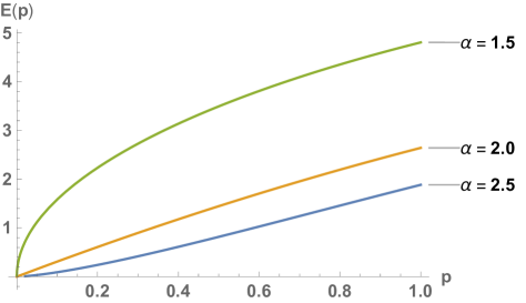
Figure S3: Dispersion relation. Plot of the dispersion relation $E(p)$ versus $p$ for $J_{0}=-1$.

Two-body system

We now introduce a single-site deep trapping potential with large coefficient $u>0$ at some site $i_{0}$ that traps and immobilizes one hardcore boson at that site,

$$U_{i}=-\sum_{j\neq i}\frac{J_{0}}{|r_{i}-r_{j}|^{\alpha}}-u\delta_{i,i_{0}}.$$ (18)

We also subtract a constant from the Hamiltonian so that the energy of the trapped boson is exactly zero. We then consider the dynamics of a second boson that feels the interactions with this fixed boson at $i_{0}$. In order to simplify our notation, let the position of the fixed boson be $r_{i_{0}}=0$. Let us now set $\beta=\alpha-1$. Then at low energies, our low-energy Hamiltonian for the second boson has the form

$$H(p,r)=2J_{0}\sin(\alpha\pi/2)\Gamma(1-\alpha)|p|^{\alpha-1}+\frac{V_{0}}{|r|^{\alpha-1}},$$ (19)

with corrections of size $O(p^{2})$. This follows from the result for $E(p)$ in Eq. (17) and that the interaction between the particles has the form $V_{ij}=V_{0}/|r_{i}-r_{j}|^{\beta}=V_{0}/|r_{i}-r_{j}|^{\alpha-1}$. We note that this Hamiltonian has classical scale invariance.

We define by analytic continuation the Fourier transforms of the functions $|r|^{\eta}$,

$$\frac{1}{\sqrt{2\pi}}\int_{-\infty}^{\infty}dre^{ipr}|r|^{\eta}=-\sqrt{\frac{2}{\pi}}|p|^{-1-\eta}\Gamma(1+\eta)\sin(\eta\pi/2).$$ (20)

We also compute the Fourier transforms of $\operatorname{sgn}(r)|r|^{\eta}$, where $\operatorname{sgn}(r)$ is the sign function,

$$\frac{1}{\sqrt{2\pi}}\int_{-\infty}^{\infty}dre^{ipr}\operatorname{sgn}(r)|r|^{\eta}=i\sqrt{\frac{2}{\pi}}\operatorname{sgn}(p)|p|^{-1-\eta}\Gamma(1+\eta)\cos(\eta\pi/2).$$ (21)

In the zero energy limit, the quantum Hamiltonian $H(p,r)$ exhibits a renormalization-group limit cycle with even-parity $(+)$ and odd-parity $(-)$ wave functions at zero energy,

$$\psi_{\rm+}(r) =\frac{1}{2}\left(|r|^{i\delta_{+}}+|r|^{-i\bar{\delta}_{+}}\right),$$ (22)

$$\psi_{\rm-}(r) =\frac{1}{2}\operatorname{sgn}(r)\left(|r|^{i\delta_{-}}+|r|^{-i\bar{\delta}_{-}}\right),$$ (23)

where $\delta_{\pm}$ are solutions to the constraints,

$$2J_{0}\delta_{+}\Gamma(1-\alpha)\sin(\alpha\pi/2)\Gamma(i\delta_{+})\sinh(\delta_{+}\pi/2) =V_{0}\Gamma(2-\alpha+i\delta_{+})\cos((\alpha-i\delta_{+})\pi/2),$$ (24)

$$2J_{0}\delta_{-}\Gamma(1-\alpha)\sin(\alpha\pi/2)\Gamma(i\delta_{-})\cosh(\delta_{-}\pi/2) =iV_{0}\Gamma(2-\alpha+i\delta_{-})\sin((\alpha-i\delta_{-})\pi/2).$$ (25)

For the particular case $\alpha=2$, this constraint simplifies to

$$\delta_{+}=\frac{V_{0}}{J_{0}\pi}\coth(\delta_{+}\pi/2),\;\;\delta_{-}=\frac{V_{0}}{J_{0}\pi}\tanh(\delta_{-}\pi/2).$$ (26)

These solutions for the case $\alpha=2$ are real whenever $V_{0}/J_{0}$ is positive. When $V_{0}/J_{0}\gg\pi$, these are both very well approximated by

$$\delta_{+}\approx\delta_{-}\approx\frac{V_{0}}{J_{0}\pi}.$$ (27)

In the cases where $\delta_{+}$ and $\delta_{-}$ are real, the discrete scale invariance of the renormalization-group limit cycle can be seen by writing

$$\psi_{\rm{+}}(r)=\cos[\delta_{+}\ln(|r|)],\;\;\;\psi_{\rm{-}}(r)=\operatorname{sgn}(r)\cos[\delta_{-}\ln(|r|)].$$ (28)

Under the scale transformations $r\rightarrow\lambda_{\pm}r,$ we have

$$\psi_{\rm{+}}(r) \rightarrow\cos[\delta_{+}\ln(|r|)+\delta_{+}\ln(\lambda_{+})],$$ (29)

$$\psi_{\rm{-}}(r) \rightarrow\operatorname{sgn}(r)\cos[\delta_{-}\ln(|r|)+\delta_{-}\ln(\lambda_{-})].$$ (30)

The wave functions remain invariant up to an overall minus sign if we let

$$\lambda_{+}=\exp(\pi/\delta_{+}),\;\;\lambda_{-}=\exp(\pi/\delta_{-}).$$ (31)

The bound state energies also respect this discrete scale symmetry. Under the scale transformation $r\rightarrow\lambda_{\pm}r$, the energy scales as $E_{\pm}\rightarrow\lambda_{\pm}^{-1}E_{\pm}$. We therefore get an infinite tower of states $E^{(n)}_{+/-}$ obeying the geometric progression

$$E^{(n)}_{+}=\epsilon_{+}\lambda_{+}^{-n},\;\;E^{(n)}_{-}=\epsilon_{-}\lambda_{-}^{-n},$$ (32)

for some negative energy constants $\epsilon_{+/-}$. We note that the case $\alpha=2$ corresponds to a Hamiltonian of the form

$$H(p,r)=-\pi J_{0}|p|+\frac{V_{0}}{|r|},$$ (33)

which, for $J_{0}<0$ and $V_{0}<0$, is analogous to a relativistic fermion with attractive Coulomb interactions. This system is therefore directly related to the scale anomaly recently proposed in graphene for Dirac fermions and attractive Coulomb interactions Ovdat et al. (2017).

For the cases where $\delta_{+}$ and $\delta_{-}$ are not real, the wave functions at zero energy are

$$\psi_{\rm{+}}(r)=|r|^{-{\rm Im}\,\delta_{+}}\cos[{\rm Re}\,\delta_{+}\ln(|r|)],\;\;\;\psi_{\rm{-}}(r)=|r|^{-{\rm Im}\,\delta_{-}}\operatorname{sgn}(r)\cos[{\rm Re}\,\delta_{-}\ln(|r|)].$$ (34)

Under the scale transformations $r\rightarrow\lambda_{\pm}r$, the wave functions scale homogeneously if we let

$$\lambda_{+}=\exp(\pi/{\rm Re}\,\delta_{+}),\;\;\lambda_{-}=\exp(\pi/{\rm Re}\,\delta_{-}).$$ (35)

Time fractals

For the purposes of this discussion, we consider the immobile boson localized at $r=0$ as a static source and consider only the wave function of the second boson, which can occupy sites $r\neq 0$. We start with an initial state

$$|S\rangle=\sum_{n=0}^{N-1}|\psi^{(n)}_{+}\rangle,$$ (36)

where we sum over the lowest $N$ even-parity bound states $|\psi^{(n)}_{+}\rangle$ with equal weight. The phase convention for each $|\psi^{(n)}_{+}\rangle$ is chosen so that the tail of the wave function is real and positive at large $r$. This state can be decomposed into position eigenstates

$$|S\rangle=\sum_{r\neq 0}S(r)|r\rangle.$$ (37)

On a classical computer we can produce time fractals by computing the amplitude

$$A(t) ={\rm Re}[Z(t)],$$ (38)

where

$$Z(t) =\langle S|\exp(-iHt)|S\rangle.$$ (39)

The experimental realization of time fractals on a trapped ion quantum system requires more effort. In order to compute the time evolution of the state $|S\rangle$, we define a product of single-qubit rotations

$$U(\epsilon)=\prod_{r\neq 0}\exp[-i\epsilon\sigma^{y}_{r}S(r)],$$ (40)

for some infinitesmal real parameter $\epsilon$. With the immobile boson still fixed at $r=0$, let us denote the normalized state with no mobile bosons at all as $|o\rangle$. The action of $U$ on the state $|o\rangle$ produces a wave function with an indefinite number of mobile bosons. We find that

$$U(\epsilon)|o\rangle=\left[1-\frac{\epsilon^{2}}{2}\langle S|S\rangle+O(\epsilon^{3})\right]|o\rangle+\epsilon|S\rangle+O(\epsilon^{2})|X\rangle,$$ (41)

As mentioned in the main text, we have subtracted a constant from the Hamiltonian so that the energy of $|o\rangle$ is zero. Hence,

$$\langle o|\exp[-iHt]|o\rangle=\langle o|o\rangle=1.$$ (42)

We now measure

$$B(\epsilon,t)=|\langle o|U^{\dagger}(\epsilon)\exp[-iHt]U(\epsilon)|o\rangle|^{2},$$ (43)

This can be viewed as a quantum measurement of the projection operator $|o\rangle\langle o|$ on the state

$$U^{\dagger}(\epsilon)\exp[-iHt]U(\epsilon)|o\rangle.$$ (44)

If we deconstruct $B(\epsilon,t)$ into powers of $\epsilon,$ we get

$$B(\epsilon,t)=\left|1-\epsilon^{2}\langle S|S\rangle+\epsilon^{2}Z(t)+O(\epsilon^{3})\right|^{2}.$$ (45)

We then obtain

$$B(\epsilon,t) =1-2\epsilon^{2}\langle S|S\rangle+\epsilon^{2}[Z(t)+Z^{*}(t)]+O(\epsilon^{3})$$

$$=1-2\epsilon^{2}\langle S|S\rangle+2\epsilon^{2}A(t)+O(\epsilon^{3}),$$ (46)

and we can thus determine the desired amplitude $A(t)$.

To our knowledge this is the first instance of the concept of time fractals appearing in the literature. However a recent preprint Gao et al. (2019) appeared a few weeks after our preprint was posted discussing a similar concept which they called dynamical fractals.

References

- Efimov (1971) V. N. Efimov, Sov. J. Nucl. Phys. 12, 589 (1971).
- Efimov (1993) V. N. Efimov, Phys. Rev. C47, 1876 (1993).
- Bedaque et al. (1999a) P. F. Bedaque, H.-W. Hammer, and U. van Kolck, Phys. Rev. Lett. 82, 463 (1999a), eprint nucl-th/9809025.
- Bedaque et al. (1999b) P. F. Bedaque, H.-W. Hammer, and U. van Kolck, Nucl. Phys. A646, 444 (1999b), eprint nucl-th/9811046.
- Coon and Holstein (2002) S. A. Coon and B. R. Holstein, Am. J. Phys. 70, 513 (2002), eprint quant-ph/0202091.
- Kraemer et al. (2006) T. Kraemer, M. Mark, P. Waldburger, J. G. Danzl, C. Chin, B. Engeser, A. D. Lange, K. Pilch, A. Jaakkola, H.-C. Naegerl, et al., Nature 440, 315 (2006), eprint cond-mat/0512394.
- Kunitski et al. (2015) M. Kunitski et al., Science 348, 551 (2015), eprint 1512.02036.
- Bedaque et al. (2000) P. F. Bedaque, H.-W. Hammer, and U. van Kolck, Nucl. Phys. A676, 357 (2000), eprint nucl-th/9906032.
- Hagen et al. (2013) G. Hagen, P. Hagen, H. W. Hammer, and L. Platter, Phys. Rev. Lett. 111, 132501 (2013), eprint 1306.3661.
- Platter et al. (2004) L. Platter, H.-W. Hammer, and U.-G. Meißner, Phys. Rev. A70, 052101 (2004), eprint cond-mat/0404313.
- Hammer and Platter (2007) H. W. Hammer and L. Platter, Eur. Phys. J. A32, 113 (2007), eprint nucl-th/0610105.
- von Stecher et al. (2009) J. von Stecher, J. P. D’Incao, and C. H. Greene, Nat. Phys. 5, 417 (2009).
- von Stecher (2011) J. von Stecher, Phys. Rev. Lett. 107, 200402 (2011), eprint 1106.2319.
- Carlson et al. (2017) J. Carlson, S. Gandolfi, U. van Kolck, and S. A. Vitiello, Phys. Rev. Lett. 119, 223002 (2017), eprint 1707.08546.
- Nishida and Tan (2011) Y. Nishida and S. Tan, Few Body Syst. 51, 191 (2011), eprint 1104.2387.
- Moroz et al. (2013) S. Moroz, Y. Nishida, and D. T. Son, Phys. Rev. Lett. 110, 235301 (2013), eprint 1301.4473.
- Happ et al. (2019) L. Happ, M. Zimmermann, S. I. Betelu, W. P. Schleich, and M. A. Efremov, arXiv e-prints arXiv:1904.07544 (2019), eprint 1904.07544.
- Nishida et al. (2013) Y. Nishida, Y. Kato, and C. D. Batista, Nature Phys. 9, 93 (2013), eprint 1208.6214.
- Nishida and Lee (2012) Y. Nishida and D. Lee, Phys. Rev. A86, 032706 (2012), eprint 1202.3414.
- Ovdat et al. (2017) O. Ovdat, J. Mao, Y. Jiang, E. Y. Andrei, and E. Akkermans, Nat. Comm. 8, 507 (2017), eprint 1701.04121.
- Zhang et al. (2017a) J. Zhang, P. W. Hess, A. Kyprianidis, P. Becker, A. Lee, J. Smith, G. Pagano, I. D. Potirniche, A. C. Potter, A. Vishwanath, et al., Nature 543, 217 (2017a), URL http://dx.doi.org/10.1038/nature21413.
- Zhang et al. (2017b) J. Zhang, G. Pagano, P. W. Hess, A. Kyprianidis, P. Becker, H. Kaplan, A. V. Gorshkov, Z. X. Gong, and C. Monroe, Nature 551, 601 (2017b), URL http://dx.doi.org/10.1038/nature24654.
- Weierstrass (1886) K. Weierstrass, Abhandlungen aus der Functionenlehre (Springer, Berlin, 1886).
- Hardy (1916) G. H. Hardy, Trans. Amer. Math. Soc. 17, 301 (1916).
- Hunt (1998) B. R. Hunt, Proc. Amer. Math. Soc. 126, 791 (1998), ISSN 0002-9939, URL https://doi.org/10.1090/S0002-9939-98-04387-1.
- Kaplan et al. (1984) J. L. Kaplan, J. Mallet-Paret, and J. A. Yorke, Ergod. Th. Dynam. Sys. 4, 261 (1984).
- Gao et al. (2019) C. Gao, H. Zhai, and Z.-Y. Shi, arXiv e-prints arXiv:1901.06983 (2019), eprint 1901.06983.