A convergence analysis of Generalized Multiscale Finite Element Methods

Abstract

In this paper, we consider an approximation method, and a novel general analysis, for second-order elliptic differential equations with heterogeneous multiscale coefficients. We obtain convergence of the Generalized Multi-scale Finite Element Method (GMsFEM) method that uses local eigenvectors in its construction. The analysis presented here can be extended, without great difficulty, to more sophisticated GMsFEMs. For concreteness, the obtained error estimates generalize and simplify the convergence analysis of [J. Comput. Phys. 230 (2011), 937-955]. The GMsFEM method construct basis functions that are obtained by multiplication of (approximation of) local eigenvectors by partition of unity functions. Only important eigenvectors are used in the construction. The error estimates are general and are written in terms of the eigenvalues of the eigenvectors not used in the construction. The error analysis involve local and global norms that measure the decay of the expansion of the solution in terms of local eigenvectors. Numerical experiments are carried out to verify the feasibility of the approach with respect to the convergence and stability properties of the analysis in view of the good scientific computing practice.

1 Introduction

Approximation of partial differential equations posed on domains with multiscale and heterogeneous properties appear in variety of applications. For instance, when modeling subsurface flow scenarios, subsurface properties typically vary several orders of magnitude over multiple scales. In this case, the high-contrast in the properties such as permeability raises additional issues to be consider when constructing approximation of solutions. Several multiscale models to efficiently solve flow and transport processes have been considered. In despite of many contributions, the design and mathematical analysis of high-contrast multiscale problems continue being a challenging problem; See for instance [1, 2, 3, 4, 5, 6, 7, 8, 9, 10, 11, 12, 13, 14, 15, 16, 17, 18]. These approaches approximate the effects of the fine-scale features using a coarse mesh. They attempt to capture the fine scale effects on a coarse grid via localized basis functions. The main idea of Multiscale Finite Element Methods (MsFEMs) is to construct basis functions that are used to approximate the solution on a coarse grid. The accuracy of MsFEMs is found to be very sensitive to the particularities of the construction of the basis functions (e.g., boundary conditions of local problems). See for instance [13, 19, 20]).

It is known that the construction of the basis functions need to be carefully designed in order to obtain accurate coarse-scale approximations of the solution (e.g., [13]). In particular, the resulting basis functions need to have similar oscillatory behavior as the fine-scale solution. In classical multiscale methods, a number of approaches are proposed to construct basis functions, e.g., oversampling techniques or the use of limited global information (e.g., [1, 13]) that employs solutions in larger regions to reduce localization errors. Recently, a new and promising methodology was introduced for the construction of basis function. This methodology is referred as to Generalized Multiscale Finite Element Method (GMsFEM). The main goal of GMsFEMs is to construct coarse spaces for MsFEMs that result in accurate coarse-scale solutions. This methodology was first developed in [14, 15, 21] in connections with the robustness of domains decomposition iterative methods for solving the elliptic equation with heterogeneous coefficients subjected to appropriate boundary conditions

$$-\mbox{div}(\kappa(x)\nabla u)=f,$$ (1)

where $\kappa(x)$ is a heterogeneous scalar field with high-contrast. In particular, it is assumed that $\kappa(x)\geq c_{0}>0$ (bounded below), while $\kappa(x)$ can have very large values.

A main ingredient in the construction was the use of local generalize eigenvalue problems and (possible multiscale) partition of unity functions to construct the coarse spaces. Besides using one coarse function per coarse node, in the GMsFEM it was proposed to use several multiscale basis functions per coarse node. These basis functions represent important features of the solution within a coarse-grid block and they are computed using eigenvectors of an eigenvalue problem. Then, in the works [22, 23, 24, 25], some studies of the coarse approximation properties of the GMsFEM were carried out. In these works and for applications to high-contrast problems, methodologies to keep small the dimension of the resulting coarse space were successfully proposed. The use of coarse spaces that somehow incorporates important modes of a (local) energy related to the problem motivated the general version of the GMsFEM. Thus,a more general and practical GMsFEM was then developed in [26] where several (more practical) options to compute important modes to be include in the coarse space was used. See also [27] for an earlier construction. It is important to mention that the methodology in [26] was designed for parametric and nonlinear problems and can be applied for variety of applications as it have been shown in recent developments not review here.

In this paper, we prove convergence of the GMsFEM method that uses local eigenvectors as developed in [23, 14, 15, 21]. The analysis presented here can be extended, without great difficulty, to more sophisticated GMsFEMs. Some convergence analysis of the GMsFEM, using local eigenvectors or approximation of them was obtained in [22]. The prove, as usual in finite element analysis, focuses on constructing interpolation operator to the coarse finite element space. The a priory error is obtained for square integrable right hand side $f$ in (2). Additionally, in [22] the authors make some assumptions concerning integrability of residuals and also concerning boundedness of the quotients of local energy norms with weight $\kappa$ and $\kappa\chi^{2}$ where $\chi^{2}$ is a especial partition of unity function. These assumptions are hard to verify in practice. Moreover, in the analysis they use a Caccioppoli inequality to write energy estimates from a region to a bigger region. Therefore, extensions of the analysis in [22] to other equations and/or different discretization is not straightforward.

In this paper, we substantially simplify the analysis of GMsFEM methods and remove the assumptions used in [22] to obtain convergence, yielding a general convergence proof and more suited for computational practice. We assume square integrability of the right hand side $f$. In order to obtain error bounds in terms of the decay of the eigenvalues used in the construction we assume that the problem is regular in the sense that the solution can be well approximated by local eigenvectors which in the case of smooth coefficients, square integrable right hand side and convex domains, is implied by the classical regularity of the problem.

It is worth to mention a main difference between the classical finite element analysis and the analysis of GMsFEM procedures for the case of heterogeneous multiscale coefficients. In the usual finite element analysis, to write the interpolation error estimates, it is assumed that the solution is smooth enough or regular enough in the classical (Sobolev) sense. This is done while using Hilbert norms (at least for elliptic problems). In the case of discontinuous multiscale coefficients, it is well know that solutions are not smooth in the classical sense. Then, the classical finite element analysis arguments do not work. In this paper, we are able to write interpolation error estimates using norms suitable for the problem at hand. In particular, to measure the “smoothness” of the solution we use the decay of the expansion of the solution in terms of global eigenvectors. This is motivated by the fact that, for a given elliptic operator, the eigenvectors are a good model for smooth functions in the scale of norms generated by powers of the operator. We define then global norms, using the decay of the expansion over global eigenvectors. We also define local norms using the decay of the expansion in terms of local eigenvectors (computed locally in a coarse node neighborhood). The main result of this paper is that we can compare the new local and global norms. With this new norms, we are able to write approximation results for the interpolation of functions that solve (2) with square integrable right hand side. We also prove error estimates in terms of the eigenvalues of the eigenvalue problem used in the construction.

The rest of the paper is organized as follow. In Section 2 we present some preliminaries on multiscale methods. In Section 3 we collect some facts on the global eigenvalue problem related to the problem. Here we introduce a scale of global norms used for the analysis. These norms measure the decay of the expansion in terms of global eigenvectors. In Sections 5 and 4 we study the local eigenvalue problems also using norms that measure the decay of the expansion in terms of the local eigenvectors. We also relate local norms to the boundary values of the eigenvalue problem. In Section 6 we review a very particular realization of the GMsFEM methodology that is the one analyzed in this paper. In Section 8 we obtain our interpolation error for the resulting method. We also write our convergence result. We present some numerical experiments in Section 9. Our numerical results verify our theoretical findings for smooth coefficients. We also consider a more practical case with heterogeneous multiscale coefficients. Finally, in Section 10 we draw some conclusions and make some final comments.

2 Preliminaries on multiscale finite element methods

In this section, we describe multiscale finite element method framework. In general terms, the MsFEMs compute the coarse-scale solution by using multiscale basis functions. It can be casted as a numerical upscaling procedure. Also as a numerical homogenization method where, instead of effective parameters representing small scale effects, basis functions are constructed that capture the small scale effects on solutions.

Multiscale techniques can be applied to variety of problems. In this paper, in order to fix ideas, we consider a second order elliptic problem with a possible multiscale high-contrast coefficient. More precisely, let $\Omega\subset\mathbb{R}^{2}$ (or $\mathbb{R}^{3}$) be a polygonal domain. We consider the elliptic equation with heterogeneous coefficients

$$-\mbox{div}(\kappa(x)\nabla u)=f,$$

where $\kappa(x)$ is a heterogeneous scalar field with high-contrast. In particular, we assume that $\kappa(x)\geq c_{0}>0$ (bounded below), while $\kappa(x)$ can have very large values. We assume that $\kappa\ inL^{\infty}({\Omega})$ and therefore $\kappa$ might be discontinuous. The variational formulation of this problem is: Find $u\in H_{0}({\Omega})$ such that

$$a(u,v)=f(v)\quad\mbox{ for all }v\in H_{0}^{1}({\Omega}).$$ (2)

Here the bilinear form $a$ and the linear functional $f$ are defined by

$$a(u,v)=\int_{\Omega}\kappa(x)\nabla u(x)\nabla v(x)dx\quad\mbox{ for all }u,v\in H_{0}^{1}({\Omega})$$

and

$$f(v)=\int_{\Omega}f(x)v(x)dx\quad\mbox{ for all }v\in H_{0}^{1}({\Omega}).$$

Let $\mathcal{T}^{H}$ be a triangulation composed by elements $K$. We refer to the triangulation $\mathcal{T}^{H}$ as a coarse triangulation in the sense that does not necessarily resolve all the scales in the model (in our case that would be all variations and discontinuities of $\kappa$). We denote $\{y_{i}\}_{i=1}^{N_{v}}$ the vertices of the coarse mesh $\mathcal{T}^{H}$ and define the neighborhood of the node $y_{i}$ by

$$\omega_{i}=\bigcup\{K\in\mathcal{T}^{H};\leavevmode\nobreak\ \leavevmode\nobreak\ \leavevmode\nobreak\ y_{i}\in\overline{K}\}.$$

and the neighborhood of an element $K$ by,

$$\omega^{K}=\bigcup\{w_{i}\leavevmode\nobreak\ \leavevmode\nobreak\ ;\leavevmode\nobreak\ \leavevmode\nobreak\ \leavevmode\nobreak\ K\subset w_{i}\}.$$ (3)

Using the coarse mesh $\mathcal{T}^{H}$ we introduce coarse basis functions $\{\Phi_{i}\}_{i=1}^{N_{c}}$, where $N_{c}$ is the number of coarse basis functions. In our paper, the basis functions are supported in $\omega_{i}$; however, for $\omega_{i}$, there may be multiple basis functions. MsFEMs approximate the solution on a coarse grid as $u_{0}=\sum c_{i}\Phi_{i}$, where $c_{I}$ are determined from

$$a(u_{0},v)=f(v),\quad\text{for all}\ v\in\text{span}\{\Phi_{i}\}_{i=1}^{N_{c}}.$$

Once $c_{i}$’s are determined, one can define a fine-scale approximation of the solution by reconstructing via basis functions, $u_{0}=\sum_{i=1}^{N_{c}}c_{i}\Phi_{i}$.

3 Global eigenvalue problem

In this section, we recall some facts about the global eigenvalue problem associated to problem (1). We stress that the global eigenvalue problem is used in the analysis only and it is not use in the computations.

We start the presentation by introducing the global mass bilinear form. This is given by

$$m(v,w)=\int_{\Omega}\kappa vw\quad\mbox{ for all }v,w\in H^{1}_{0}(\Omega).$$

Note that we use the coefficient $\kappa$ in the mass matrix. The reason is that our main application in mind is on high-contrast problems and, as show in [25, 28, 14, 15], it is important to define the mass matrix with the coefficient $\kappa$. Moreover, more complicated bilinear forms can be also used as in recent developments in GMsFEM; see [26, 29].

We consider the eigenvalue problem (in weak form) that seeks to find eigenfunctions $\phi$ and scalars $\mu$ such that

$$a(\phi,z)=\mu m(\phi,z)\quad\mbox{ for all }z\in H_{0}^{1}({\Omega}).$$ (4)

Denote it’s eigenvalues and eigenfunctions by $\{\mu_{\ell}\}$ and $\{\phi_{\ell}\}$, respectively. We order eigenvalues as

$$\mu_{1}\leq\mu_{2}\leq\dots\leq\mu_{\ell}\dots.$$ (5)

We have $\mu_{1}>0$. The eigenvalue problem (4) is the weak form of the eigenvalue problem

$$-\mbox{div}(\kappa\nabla\phi)=\mu\kappa\phi$$ (6)

in ${\Omega}$ with homogeneous Dirichlet boundary condition on $\partial{\Omega}$.

We recall that the eigenvectors form a complete ($m$)-orthonormal system of $L^{2}({\Omega})$ that is also orthogonal with respect to the bilinear form $a$. Given any $v\in H^{1}_{0}(\Omega)$ we can write

$$v=\sum_{\ell=1}^{\infty}m(v,\phi_{\ell})\phi_{\ell}$$

and compute the bilinear form $a$ as

$$a(v,v)=\sum_{\ell=1}^{\infty}\mu_{\ell}m(v,\phi_{\ell})\phi_{\ell}$$ (7)

and the bilinear form $m$ as

$$m(v,v)=\sum_{\ell=1}^{\infty}m(v,\phi_{\ell})^{2}.$$ (8)

It is important to recall that the expansion of the solution can be explicitly given. In fact, from the weak form (2) we see that

$$\mu_{\ell}m(u,\phi)=a(u,\phi)=f(\phi).$$

Then we have

$$u=\sum_{\ell=1}^{\infty}\frac{1}{\mu_{\ell}}f(\phi_{\ell})\phi_{\ell}.$$ (9)

The eigenvector are the regular functions par excellence when working with the differential operator $-\mbox{div}(\kappa\nabla\cdot)$. In particular we stress the following fact.

Remark 1

We have that $\kappa\nabla\phi_{\ell}$ has a square integrable divergence. That is, $-\mbox{div}(\kappa\nabla\phi_{\ell})\in L^{2}({\Omega})$. This follows by observing that, in a generalize sense, $-\mbox{div}(\nabla\phi_{\ell})=\mu_{\ell}\kappa\phi_{\ell}$.

3.1 Global Norms based on eigenvalue expansion decay

In this section, we introduce a scale of norms that help measuring the decay of the expansions in terms of eigenvectors of the global eigenvalue problem. These norms are used in the a priori error estimates of our GMsFEM method. We note that, without assuming some sort of regularity of the solution of (2), it is difficult to measure the rate of the error in finite element approximations and give error estimates. For this paper, we only assume that the forcing term is square integrable in order to obtain approximation using global eigenvector. Later we consider the case of approximation using locally constructed basis functions with small support that employ local eigenvector in its design.

For any $v\in L^{2}({\Omega})$ written as $v=\sum_{\ell=1}^{\infty}m(v,\phi_{\ell})\phi_{\ell}$ and $s>0$, we introduce the norm $|||\cdot|||_{s;{\Omega}}$ defined by,

$$|||v|||_{s;{\Omega}}^{2}=\sum_{\ell=1}^{\infty}\mu_{\ell}^{s}m(v,\phi_{\ell})^{2}.$$

We note that these norms depend on the bilinear forms $a$ and $m$ but, in order to make notation simpler, we do not stress this dependence in our notation. Note that

$$|||v|||_{0;{\Omega}}^{2}=m(v,v)=\int_{\Omega}\kappa v^{2}\quad\mbox{ and }\quad|||v|||_{1;{\Omega}}^{2}=a(v,v)=\int_{\Omega}\kappa|\nabla v|^{2}.$$

In this paper, we mainly use the norm $|||\cdot|||_{s;{\Omega}}$ with $s=2$. We have that

$$|||u|||_{2;{\Omega}}^{2}=\sum_{\ell=1}^{\infty}\mu_{\ell}^{2}m(v,\phi_{\ell})^{2}.$$

Then, if $|||u|||_{2;{\Omega}}<\infty$ we can define the operator $\mathcal{A}$ applied to $u$ by

$$\mathcal{A}u=\sum_{\ell=1}^{\infty}\mu_{\ell}m(u,\phi_{\ell})\phi_{\ell}.$$

We readily have $\mathcal{A}u\in L^{2}({\Omega})$ since,

$$|||\mathcal{A}u|||_{0;{\Omega}}^{2}=m(\mathcal{A}u,\mathcal{A}u)=\sum_{\ell=1}^{\infty}\mu_{\ell}^{2}m(u,\phi_{\ell})^{2}=|||u|||_{2;{\Omega}}^{2}<\infty.$$

Furthermore, if $|||u|||_{2;{\Omega}}<\infty$ we also have the following integration by parts relation, that can be verified by straightforward calculations,

$$a(u,v)=m(\mathcal{A}u,v)\quad\mbox{ for all }v\in H_{0}^{1}({\Omega}).$$ (10)

We now present a characterization of $\mathcal{A}$ using the divergence operator div and the coefficient $\kappa$. This implies that for even integer values of $s$ (in particular for $s=2$), the norm $|||\cdot|||_{s}$ is computed by subassembly of similar norms in subdomains.

Theorem 2

The operator $\mathcal{A}$ is a locally defined operator. More precisely, if $|||u|||_{2;{\Omega}}<\infty$ we have that $-\kappa^{-1}\mbox{div}(\kappa\nabla u)$ belongs to the space $L^{2}({\Omega})$ and we have

$$\mathcal{A}u=-\kappa^{-1}\mbox{div}(\kappa\nabla u).$$

Moreover, we have

$$|||u|||^{2}_{2;{\Omega}}=\|\mathcal{A}u\|_{0}^{2}=\int_{\Omega}\kappa^{-1}|\mbox{div}(\kappa\nabla u)|^{2}.$$

Proof. Recall that for $u\in L^{2}({\Omega})$, we have the expansion $u=\sum_{\ell=1}^{\infty}m(u,\phi_{\ell})\phi_{\ell}.$ For an integer $N$ define the truncated approximation of $u$ as,

$$u^{N}=\sum_{\ell=1}^{N}m(u,\phi_{\ell})\phi_{\ell}.$$

We construct the $-\kappa^{-1}\mbox{div}(\kappa\nabla u)$ as a limit in the $m-$norm of the sequence of rescaled divergences given by $\{\kappa^{-1}\mbox{div}(\kappa\nabla u^{N})\}_{N=1}^{\infty}$. To this end, we prove that the sequence $\{\kappa^{-1}\mbox{div}(\kappa\nabla u^{N})\}_{N=1}^{\infty}$ is a Cauchy sequence in the $m-$norm. Indeed, we have, by using the eigenvalue problem (6) and Remark 1, the following identity,

$$\kappa^{-1}\mbox{div}(\kappa\nabla u^{N})=\sum_{\ell=1}^{N}m(u,\phi_{\ell})\mu_{\ell}\phi_{\ell}.$$

So that, using the orthogonality of the eigenvectors, we conclude that for every $M>N$ we have,

$$\|\kappa^{-1}\mbox{div}(\kappa\nabla u^{M})-\kappa^{-1}\mbox{div}(\kappa\nabla u^{N})\|_{0}^{2}=\sum_{\ell=N+1}^{M}m(u,\phi_{\ell})^{2}\mu_{\ell}^{2}.$$

This implies the claim since the series $|||u|||^{2}_{2;{\Omega}}=\sum_{\ell=1}^{\infty}m(u,\phi_{\ell})^{2}\mu_{\ell}^{2}<\infty$. We conclude that there exist an $L^{2}({\Omega})$ function, denoted by $U$, such that we have $\|U+\kappa^{-1}\mbox{div}(\kappa\nabla u^{N})\|\to 0$ when $N\to\infty$. We also have that for any $z\in H^{1}_{0}({\Omega})$ it holds,

$$\int_{\Omega}\kappa Uz=-\lim_{N\to\infty}\int_{\Omega}\kappa\kappa^{-1}\mbox{div}(\kappa\nabla u^{N})z=\int_{\Omega}\kappa\nabla u\nabla z,$$

which proves that $U=-\kappa^{-1}\mbox{div}(\kappa\nabla u^{N})z$.

Finally note that, by using (10), for every function $z\in H^{1}_{0}({\Omega})$ we have,

$$\int_{\Omega}\kappa\mathcal{A}uz=m(\mathcal{A}u,v)=a(u,z)=\int_{\Omega}\kappa\nabla u\nabla z.$$

 

Remark 3

Notice that if $u$ is the solution of (2) with $f\in L^{2}({\Omega})$, then, we have $\mathcal{A}u=\kappa^{-1}f$.

Lemma 4

Assume that $|||f|||_{s}^{2}<\infty$ and let $u$ be the solution of (2). Consider $t\geq 1$ such that $t-s-2\leq 0$ we have

$$|||u|||^{2}_{t}\leq\mu^{t-s-2}_{1}|||f|||_{s}^{2}$$

In particular, if $|||f|||_{0}<\infty$ we have that $|||u|||_{2}=|||\kappa^{-1}f|||_{0}=\int_{\Omega}\kappa^{-1}f^{2}$.

Proof. Using the explicit expansion in (9), the definition of the norm $\|\cdot\|_{t}$ and then increasing the order of eigenvalues we have

$$|||u|||^{2}_{t} =\sum_{\ell=1}^{\infty}\mu^{t}_{\ell}\frac{1}{\mu_{\ell}^{2}}f(\phi_{\ell})^{2}=\sum_{\ell=1}^{\infty}\mu^{t-s-1}_{\ell}\mu^{s}_{\ell}f(\phi_{\ell})^{2}$$

$$\leq\mu^{t-s-2}_{0}\sum_{\ell=1}^{\infty}\mu^{s}_{\ell}f(\phi_{\ell})^{2}$$

$$=\mu^{t-s-2}_{0}\sum_{\ell=1}^{\infty}\mu^{s}_{\ell}\left(\int_{\Omega}f\phi_{\ell}\right)^{2}$$

$$=\mu^{t-s-2}_{0}\sum_{\ell=1}^{\infty}\mu^{s}_{\ell}\left(\int_{\Omega}\kappa(\kappa^{-1}f)\phi_{\ell}\right)^{2}=\mu^{t-s-2}_{0}|||\kappa^{-1}f|||_{s}^{2}.$$

This finishes the proof.  

3.2 Approximation using global eigenvectors

In this section, we show how to obtain a priori error estimates if we use the space spanned by the first eigenvectors. Given an integer $L$ and $v\in H^{1}_{0}(\Omega)$, we define

$$\mathcal{J}_{L}v=\sum_{\ell=1}^{L}m(v,\phi_{\ell})\phi_{\ell}.$$

From (5), (7), and (8) it is easy to prove the following inequality

$$\int_{\Omega}\kappa(v-\mathcal{J}_{L}v)^{2}\leq\frac{1}{\mu_{L+1}}a(v-\mathcal{J}_{L}v,v-\mathcal{J}_{L}v)\leq\frac{1}{\mu_{L+1}}a(v,v).$$ (11)

When ${L}=1$ and $\kappa=1$ we obtain the usual Friedrichs’ inequality.

If $u$ is the solution of (2) and $|||f|||_{s}<\infty$ we have the following a priori estimate.

Lemma 5

Let $u$ be the solution of (2). If if $t-s-2<0$ we have

$$|||u-\mathcal{J}_{L}u|||^{2}_{t}\leq\mu^{t-s-2}_{L+1}|||f|||_{s}^{2}.$$

Proof. Using the explicit expansion in (9), the definition of the norm $\|\cdot\|_{t}$ and then increasing oder of eigenvalues we have

$$|||u-\mathcal{J}_{L}u|||^{2}_{t} =\sum_{\ell={L}+1}^{\infty}\mu^{t}_{\ell}\frac{1}{\mu_{\ell}^{2}}f(\phi_{\ell})^{2}=\sum_{\ell=L+1}^{\infty}\mu^{t-s-2}_{\ell}\mu^{s}_{\ell}f(\phi_{\ell})^{2}$$

$$\leq\mu^{t-s-2}_{L+1}\sum_{\ell=1}^{\infty}\mu^{s}_{\ell}f(\phi_{\ell})^{2}=\mu^{t-s-2}_{L+1}|||f|||_{s}^{2}.$$

This finishes the proof.  

We observe that, in particular, we have the following a priori error estimates.

$$a(u-\mathcal{J}_{L}u,u-\mathcal{J}_{L}u)=|||u-\mathcal{J}_{L}u|||^{2}_{1}\leq\lambda^{-(s+1)}_{L+1}|||f|||_{s}^{2}.$$

The space generated by the first eigenvalues gives good approximation spaces and the analysis becomes easy.

4 Dirichlet eigenvalue problem in coarse blocks

In this section, we study the local Dirichlet eigenvalue problem associated to problem (1). For any $K$, we define the following bilinear forms

$$a^{K}(v,w)=\int_{K}\kappa\nabla v\nabla w\quad\mbox{ for all }v,w\in H^{1}(K),\quad i=1,\dots,N,$$

and

$$m^{K}(v,w)=\int_{K}\kappa vw\quad\mbox{ for all }v,w\in H^{1}(K).$$

We consider the eigenvalue problems that seek eigenfunctions $\phi\in H^{1}_{0}(K)$ and scalars $\mu$ such that

$$a^{K}(\phi,z)=\mu m^{K}(\phi,z)\quad\mbox{ for all }z\in H^{1}_{0}(K).$$

and denote its eigenvalues and eigenvectors by $\{\mu_{\ell}^{K}\}$ and $\{\phi_{\ell}^{K}\}$, respectively. Note that the eigenvectors $\{\phi^{K}_{\ell}\}$ form an orthonormal basis of $L^{2}(K)$ with respect to the $m^{K}$ inner product. We order eigenvalues as

$$\mu_{1}^{K}<\mu_{2}^{K}\leq\dots\leq\mu_{\ell}^{K}\dots.$$

The eigenvalue problem above corresponds to the approximation of the eigenvalue problem

$$-\mbox{div}(\kappa\nabla\phi)=\mu\kappa\phi\quad\mbox{ in }K,$$ (12)

with homogeneous Dirichlet boundary condition on $\partial K$. These eigenvectors are the model of regular functions working with the differential operator $-\mbox{div}(\kappa\nabla\cdot)$. In particular, the operator is well defined and well behaved over these functions. We have that $\kappa\nabla\phi^{K}_{\ell}$ has a square integrable divergence. That is, $-\mbox{div}(\nabla\phi^{K}_{\ell})\in L^{2}(K)$. This follows by observing that, in a generalize sense, $-\mbox{div}(\nabla\phi_{\ell})=\mu_{\ell}\kappa\phi_{\ell}$.

Now we use the expansion in terms of local eigenvectors and define norms based on the decay of the eigenexpansion. These local norms are the ones that naturally appear in the local interpolation errors for our interpolation operator. A main issue is to compare this local norms with the global norms defined in Section 3.1 for $s>1$. For the case $s=2$, we prove in Theorem 6 that the local norms can be assembled to obtain a global norms equivalent to the norm $|||\cdot|||_{2,\Omega}$ only for functions that have zero value on block boundaries.

Given any $v\in L^{2}(K)$ we can write

$$v=\sum_{\ell=1}^{\infty}m^{K}(v,\phi_{\ell}^{K})\phi_{\ell}^{K}$$

and compute the local energy bilinear form by

$$a^{K}(v,v)=\sum_{\ell=1}^{\infty}m^{K}(v,\phi_{\ell}^{K})^{2}\mu_{\ell}^{K}.$$

We can also compute the local mass bilinear as,

$$m^{K}(v,v)=\sum_{\ell=1}^{\infty}m^{K}(v,\phi_{\ell}^{K})^{2}.$$

The local norm to measure the decay of the expansion is introduced as follows. We introduce the norm,

$$|||v|||_{s,K}^{2}=\sum_{\ell=1}^{\infty}(\mu_{\ell}^{K})^{s}m^{K}(v,\phi_{\ell}^{K})^{2}.$$

Note that

$$|||v|||_{0;K}^{2}=m(v,v)=\int_{K}\kappa v^{2}\quad\mbox{ and }\quad|||v|||_{1;K}^{2}=\int_{K}\kappa|\nabla v|^{2}.$$

We consider the case $s=2$. If $|||u|||_{2,K}<\infty$ we can define the operator $\mathcal{A}^{K}$ by,

$$\mathcal{A}^{K}u=\sum_{\ell=1}^{\infty}\mu_{\ell}^{K}m^{K}(u,\phi_{\ell}^{K})\phi_{\ell}^{K}$$

which is square integrable since

$$|||\mathcal{A}^{K}u|||_{0,K}^{2}=\sum_{\ell=1}^{\infty}(\mu_{\ell}^{K})^{2}m^{K}(u,\phi_{\ell}^{K})^{2}=|||u|||_{2,K}^{2}.$$

Additionally if $|||u|||_{2,K}<\infty$, we have the following local integration by parts relation that can be verified by direct calculations,

$$a^{K}(u,v)=m^{K}(\mathcal{A}^{K}u,v)\mbox{ for all }v\in H^{1}_{0}(K).$$

We have the following result. This result reveals that the local norms $|||u|||_{2,K}$ is related to the $L^{2}$ integrability of $\mbox{div}(\kappa\nabla\cdot u)$. The proof of the following theorem follows the proof of Theorem 2 but we presented in the local setting in the interest of completeness.

Theorem 6

The operator $\mathcal{A}^{K}$ is a locally defined operator. More precisely, if $|||u|||^{2}_{2,K}<\infty$ we have that $-\kappa^{-1}\mbox{div}(\kappa\nabla u)$ belongs to the space $L^{2}(K)$ and we have

$$a^{K}(u,v)=-\int_{K}\kappa^{-1}\mbox{div}(\kappa\nabla u)v\quad\mbox{ for all }v\in H_{0}^{1}(K).$$

Moreover, we have

$$|||u|||^{2}_{2,K}=\|\mathcal{A}^{K}u\|_{0,K}^{2}=\int_{K}\kappa^{-1}|\mbox{div}(\kappa\nabla u)|^{2}.$$

Proof. Since $u\in L^{2}(K)$ we have the expansion $u=\sum_{\ell=1}^{\infty}m^{K}(u,\phi_{\ell}^{K})\phi_{\ell}^{K}$. For any integer $N$, truncate this expansion to get,

$$u^{N}:=\sum_{\ell=1}^{N}m^{\omega_{i}}(u,\phi_{\ell}^{K})\phi_{\ell}^{K}.$$

The sequence of rescaled divergences, $\{\kappa^{-1}\mbox{div}(\kappa\nabla u^{N})\}_{N=1}^{\infty}$, is a Cauchy sequence in the $m^{K}-$norm. Indeed, we have, by using the eigenvalue problem (12), the following identity,

$$\kappa^{-1}\mbox{div}(\kappa\nabla u^{N})=\sum_{\ell=1}^{N}m^{K}(u,\phi_{\ell}^{K})\mu_{\ell}^{K}\phi_{\ell}^{K}.$$

So that, using the orthogonality of the eigenvectors we conclude that for every $M>N$ we have,

$$|||\kappa^{-1}\mbox{div}(\kappa\nabla u^{M})-\kappa^{-1}\mbox{div}(\kappa\nabla u^{N})|||_{0,{K}}^{2}=\sum_{\ell=N+1}^{M}m^{K}(u,\phi_{\ell}^{K})^{2}(\mu_{\ell}^{K})^{2}.$$

Then, there exists an $L^{2}(K)$ function, say $U$, such that $\|U+\kappa^{-1}\mbox{div}(\kappa\nabla\mu)\|_{0,{K}}\to 0$ when $N\to\infty$.

We also have that for any $z\in H^{1}_{0}(K)$ it holds,

$$\int_{K}\kappa Uz=-\lim_{N\to\infty}\int_{K}\kappa\kappa^{-1}\mbox{div}(\kappa\nabla\mu)z=\int_{K}\kappa\nabla u\nabla z,$$

which proves that $U=-\kappa^{-1}\mbox{div}(\kappa\nabla\mu)$.

Finally note that for every function $z\in H^{1}_{0}(K)$ we have,

$$\int_{K}\kappa\mathcal{A}^{K}uz=m(\mathcal{A}^{K}u,v)=a(u,z)=\int_{K}\kappa\nabla u\nabla z.$$

 

Given an integer $L$ and $v\in H^{1}_{0}(K)$, we define

$$\mathcal{J}_{L}^{K}v=\sum_{\ell=1}^{L}m(v,\phi_{\ell})\phi_{\ell}.$$

From the analogous to (5), (7), and (8) it is easy to prove the following inequality

Lemma 7

Assume that $u\in H^{1}_{0}(K)$ and $|||u|||_{s,K}\leq\infty$ with $s>1$. We have for $1\leq s\leq t\leq 2$,

$$|||u-\mathcal{J}_{L}^{K}u|||^{2}_{t,K}\leq(\mu^{K}_{L+1})^{t-s}|||u|||_{s,K}^{2}.$$

In particular,

$$|||u-\mathcal{J}_{L}^{K}u|||^{2}_{1,K}\leq\mu^{K}_{L+1}|||\mathcal{A}^{K}u|||_{0,K}^{2}.$$

5 Local Neumann eigenvalue problem in coarse neighborhoods

In this section, we study local eigenvalue problem associated to problem (1). For any $\omega_{i}$, we define the following bilinear forms

$$a^{\omega_{i}}(v,w)=\int_{\omega_{i}}\kappa\nabla v\nabla w\quad\mbox{ for all }v,w\in H^{1}(\omega_{i}),\quad i=1,\dots,N,$$

and

$$m^{\omega_{i}}(v,w)=\int_{\omega_{i}}\kappa vw\quad\mbox{ for all }v,w\in H^{1}(\omega_{i}).$$

Define $\widetilde{V}(\omega_{i})=\{v\in H^{1}(\omega_{i})\leavevmode\nobreak\ :\leavevmode\nobreak\ v=0\mbox{ on }\partial\omega_{i}\cap\partial\Omega\}$ if $\partial\omega_{i}\cap\partial\Omega$ is non-empty and $\widetilde{V}(\omega_{i})=\{v\in H^{1}(\omega_{i})\leavevmode\nobreak\ :\leavevmode\nobreak\ \int_{\omega_{i}}v=0\}$ otherwise. We consider the eigenvalue problems that seek eigenfunctions $\psi\in\widetilde{V}(\omega_{i})$ and scalars $\lambda$ such that

$$a^{\omega_{i}}(\psi,z)=\lambda m^{\omega_{i}}(\psi,z)\quad\mbox{ for all }z\in\widetilde{V}(\omega_{i}),$$

and denote its eigenvalues and eigenvectors by $\{\lambda_{\ell}^{\omega_{i}}\}$ and $\{\psi_{\ell}^{\omega_{i}}\}$, respectively. Note that the eigenvectors $\{\psi^{\omega_{i}}_{\ell}\}$ form an orthonormal basis of of $L^{2}(\omega_{i})$ with respect to the $m^{\omega_{i}}$ inner product. Note that $\lambda_{1}^{\omega_{i}}=0$ when $\partial\omega_{i}\cap\partial{\Omega}$ is empty, that is, when $\omega_{i}$ is a floating subdomain. We order eigenvalues as

$$\lambda_{1}^{\omega_{i}}<\lambda_{2}^{\omega_{i}}\leq\dots\leq\lambda_{\ell}^{\omega_{i}}\dots.$$

The eigenvalue problem above corresponds to the approximation of the eigenvalue problem

$$-\mbox{div}(\kappa\nabla v)=\lambda\kappa v\quad\mbox{ in }\omega_{i}$$ (13)

with homogeneous Neumann boundary condition on $\partial\omega_{i}\cap\Omega$ and homogeneous Dirichlet boundary condition on $\partial\omega_{i}\cap\partial\Omega$ (when non-empty).

As mentioned before when studying the global eigenvalue problem, these eigenvectors are the model of regular functions working with the differential operator $-\mbox{div}(\kappa\nabla\cdot)$. In particular the operator is well defined and well behaved over these functions. We have that $\kappa\nabla\psi_{\ell}$ has a square integrable divergence. That is, $-\mbox{div}(\nabla\psi_{\ell})\in L^{2}(\omega_{i})$. This follows by observing that, in a generalize sense, $-\mbox{div}(\nabla\psi_{\ell})=\lambda_{\ell}\kappa\psi_{\ell}$.

Given any $v\in\widetilde{V}(\omega_{i})$ we can write

$$v=\sum_{\ell=1}^{\infty}m^{\omega_{i}}(v,\psi_{\ell}^{\omega_{i}})\psi_{\ell}^{\omega_{i}}$$

and compute the local energy bilinear form by

$$a^{\omega_{i}}(v,v)=\sum_{\ell=1}^{\infty}m^{\omega_{i}}(v,\psi_{\ell}^{\omega_{i}})^{2}\lambda_{\ell}^{\omega_{i}}.$$

We can also compute the local mass bilinear as,

$$m^{\omega_{i}}(v,v)=\sum_{\ell=1}^{\infty}m^{\omega_{i}}(v,\psi_{\ell}^{\omega_{i}})^{2}.$$

The local norm to measure the decay of the expansion is introduced as follows. We introduce the semi-norm,

$$|||v|||_{s,\omega_{i}}^{2}=\sum_{\ell=1}^{\infty}(\lambda_{\ell}^{\omega_{i}})^{2s}m^{\omega_{i}}(v,\psi_{\ell}^{\omega_{i}})^{2}.$$

Note that for $s=0$ we have a norm and for $s=1$ the semi-norms becomes a norm when restricted to non-constant functions on $\omega_{i}$, more precisely,

$$|||v|||_{0;\omega_{i}}^{2}=m(v,v)=\int_{\omega_{i}}\kappa v^{2}\quad\mbox{ and }\quad|||v|||_{1;\omega_{i}}^{2}=\int_{\omega_{i}}\kappa|\nabla v|^{2}.$$

We consider the case $s=2$. If $|||u|||_{2,\omega_{i}}<\infty$ we can define the operator $\mathcal{A}^{\omega_{i}}$ by,

$$\mathcal{A}^{\omega_{i}}u=\sum_{\ell=1}^{\infty}\lambda_{\ell}^{\omega_{i}}m^{\omega_{i}}(v,\psi_{\ell}^{\omega_{i}})\psi_{\ell}^{\omega_{i}}.$$

which is square integrable since

$$|||\mathcal{A}^{\omega_{i}}u|||_{0,\omega_{i}}^{2}=\sum_{\ell=1}^{\infty}(\lambda_{\ell}^{\omega_{i}})^{2}m^{\omega_{i}}(v,\psi_{\ell}^{\omega_{i}})^{2}=|||u|||_{2,\omega_{i}}^{2}.$$

Additionally, if $|||u|||_{2,\omega_{i}}<\infty$, we have the following local integration by parts relation (that can be verified directly by the series expansion of both sides),

$$a^{\omega_{i}}(u,v)=m^{\omega_{i}}(\mathcal{A}^{\omega_{i}}u,v)\mbox{ for all }v\in H^{1}(\omega_{i}).$$ (14)

We have the following result.

Theorem 8

The operator $\mathcal{A}^{\omega_{i}}$ is a locally defined operator. More precisely, if $|||u|||^{2}_{2,\omega_{i}}<\infty$ we have that $-\kappa^{-1}\mbox{div}(\kappa\nabla u)$ belongs to the space $L^{2}(\omega_{i})$ and we have

$$a^{\omega_{i}}(u,v)=-\int_{\omega_{i}}\kappa^{-1}\mbox{div}(\kappa\nabla u)v\quad\mbox{ for all }v\in H_{0}^{1}(\omega_{i}).$$

Moreover, we have

$$|||u|||^{2}_{2,\omega_{i}}=\|\mathcal{A}^{\omega_{i}}u\|_{0,\omega_{i}}^{2}=\int_{\omega_{i}}\kappa^{-1}|\mbox{div}(\kappa\nabla u)|^{2}.$$

Proof. Since $u\in L^{2}(\omega_{i})$ we have the expansion $u=\sum_{\ell=1}^{\infty}m^{\omega_{i}}(u,\psi_{\ell}^{\omega_{i}})\psi_{\ell}^{\omega_{i}}$. For any integer $N$, truncate this expansion to get,

$$u^{N}:=\sum_{\ell=1}^{N}m^{\omega_{i}}(u,\psi_{\ell}^{\omega_{i}})\psi_{\ell}^{\omega_{i}}.$$

The sequence of rescaled divergences, $\{\kappa^{-1}\mbox{div}(\kappa\nabla u^{N})\}_{N=1}^{\infty}$, is a Cauchy sequence in the $m^{\omega_{i}}-$norm. Indeed, we have, by using the eigenvalue problem (13), the following identity,

$$\kappa^{-1}\mbox{div}(\kappa\nabla u_{N})=\sum_{\ell=1}^{N}m^{\omega_{i}}(u,\psi_{\ell}^{\omega_{i}})\lambda_{\ell}^{\omega_{i}}\psi_{\ell}^{\omega_{i}}.$$

So that, using the orthogonality of the eigenvectors we conclude that for every $M>N$ we have,

$$|||\kappa^{-1}\mbox{div}(\kappa\nabla u_{M})-\kappa^{-1}\mbox{div}(\kappa\nabla u_{N})|||_{0,{\omega_{i}}}^{2}=\sum_{\ell=N+1}^{M}m^{\omega_{i}}(u,\psi_{\ell}^{\omega_{i}})^{2}(\lambda_{\ell}^{\omega_{i}})^{2}.$$

Then, there exists an $L^{2}(\omega_{i})$ function, say $U$, such that $\|U+\kappa^{-1}\mbox{div}(\kappa\nabla u_{N})\|_{0,{\omega_{i}}}\to 0$ when $N\to\infty$. We also have that for any $z\in H^{1}_{0}(\omega_{i})$ it holds,

$$\int_{\omega_{i}}\kappa Uz=-\lim_{N\to\infty}\int_{\omega_{i}}\kappa\kappa^{-1}\mbox{div}(\kappa\nabla u_{N})z=\int_{\omega_{i}}\kappa\nabla u\nabla z,$$

which proves that $U=-\kappa^{-1}\mbox{div}(\kappa\nabla u_{N})$. Finally, note that for every function $z\in H^{1}_{0}(\omega_{i})$ we have,

$$\int_{\omega_{i}}\kappa\mathcal{A}^{\omega_{i}}uz=m(\mathcal{A}^{\omega_{i}}u,v)=a(u,z)=\int_{\omega_{i}}\kappa\nabla u\nabla z.$$

 

Remark 9

In virtue of Theorem 8 and the equality (14) we see that a necessary condition for the $L^{2}$ integrability of $\mbox{div}(\kappa\nabla u)$ is that $\kappa\partial_{\eta}u=0$ on $\partial\omega_{i}$. Note that in general, if we are not sure $|||u|||^{2}_{2,\omega_{i}}<\infty$ and we do not assume $\partial_{\eta}u=0$ then, the integration by parts become

$$a^{\omega_{i}}(u,v)-\int_{\partial\omega_{i}}\kappa\partial_{\eta}uv=-\int_{D}\mbox{div}(\kappa\nabla u)v\mbox{ for all }v\in H^{1}(\omega_{i}).$$

Therefore, doing estimates about the eigenvalue decay is harder in this case. We also mention that in the analysis presented in [22], it is assume the square integrability of $\mbox{div}(\kappa\nabla u)$ that, as mentioned above, implies $\kappa\partial_{\eta}u=0$. Assuming that the solution has zero flux across boundaries neighborhoods is not a general assumption. A main contribution of this paper is to clarify this main assumption of [22] and to present an analysis valid for the general case where the solution $u$ does not have null fluxes across neighborhood boundaries. As we show in our numerical experiments, for the case of a solution that is not close to a function with null flux across neighborhood boundaries, the convergence rate of the GMsFEM as introduced in [22] is not optimal and additional basis functions constructed from local Dirichlet eigenvalues must be introduced to recover good convergence.

Lemma 10

Assume that $u\in H^{1}(\omega_{i})$, $\partial_{n}u=0$ and $|||u|||_{s,\omega_{i}}\leq\infty$ with $s>1$. We have for $1\leq s\leq t\leq 2$,

$$|||u-\mathcal{I}_{L}^{\omega_{i}}u|||^{2}_{t,\omega_{i}}\leq(\lambda_{L+1}^{\omega_{i}})^{t-s}|||u|||_{s,\omega_{i}}^{2}.$$

In particular,

$$|||u-\mathcal{I}_{L}^{\omega_{i}}u|||^{2}_{1,\omega_{i}}\leq\lambda_{L+1}^{\omega_{i}}|||\mathcal{A}^{\omega_{i}}u|||_{0,\omega_{i}}^{2}.$$

6 GMsFEM space construction using local eigenvalue problems

In this section, we summarize the construction of coarse scale finite element spaces using a GMsFEM framework. In order to focus in the analysis of convergence we consider a particular case of the construction of spaces using the GMsFEM framework as introduced in [22, 28]. This construction evolved to the GMsFEM method as described in [26]. The method presented in this paper to obtain convergence can be also carried out for the constructions in [26] under appropriate assumptions of the local spectral problems used for the construction of coarse spaces.

We choose the basis functions that span the eigenfunctions corresponding to small eigenvalues. We note that $\{\omega_{i}\}_{y_{i}\in\mathcal{T}^{H}}$ is a covering of $\Omega$. Let $\{\chi_{i}\}_{i=1}^{N_{v}}$ be a partition of unity subordinated to the covering $\{\omega_{i}\}$ such that $\chi_{i}\in V^{h}(\Omega)$ and $|\nabla\chi_{i}|\leq\frac{1}{H}$, $i=1,\dots,N_{v}$. Define the set of coarse basis functions

$$\Phi_{i,\ell}=\chi_{i}\psi_{\ell}^{\omega_{i}}\quad\mbox{ for }1\leq i\leq N_{v}\mbox{ and }1\leq\ell\leq L_{i},$$ (15)

where $L_{i}$ is the number of eigenvalues that will be chosen for the node $i$; see [30, 31] for more details on the generalized finite element method using partitions of unity. Denote by $V_{0}$, as before, the local spectral multiscale space

$$V_{N}=\mbox{span}\{\Phi_{i,\ell}:1\leq i\leq N_{v}\mbox{ and }1\leq\ell\leq L_{i}\}.$$

Define also

$$V_{D}=\mbox{span}\{\phi_{\ell}^{K}:K\in\mathcal{T}^{H}\mbox{ and }1\leq\ell\leq L_{K}\}.$$

Finally define,

$$V_{0}=V_{N}+V_{D}.$$

In practice, the computation of the multiscale basis functions have to be done. For instance, the computation of the multiscale basis functions can be performed in a fine grid (local to each region) that is sufficiently fine to resolve and represent the scales of the problem. In our case, this means that the fine-grid have to be sufficiently fine to represent the variations and discontinuities of the coefficient $\kappa$. The computations of the basis functions are local to each coarse region and can be done in a preprocessing step (taking advantage of parallel computations). For more details and related concepts, we refer to [26].

We define $u_{H}$ as the Galerkin approximation using the space $V_{0}$, that is,

$$a(u_{H},v)=f(v),\quad\text{for all}\ v\in V_{0}.$$ (16)

7 A technical assumption

In order to get convergence rates we assume that we can decompose the exact solution $u$ as $u\approx u_{D}+u_{N}$ where the $u_{D}$ can be approximated using the space $V_{D}$ and $u_{N}$ can be approximated using the space $V_{D}$. This requires that $u_{N}$ and $u_{D}$ have the right boundary condition on the coarse block edges. See Remark 9. More precisely we estate the following assumption.

Assumption 11

Let $u$ be the exact solution, that is $-\mbox{div}(\kappa\nabla u)=f$. We assume that there exists $u_{D}$, $u_{N}$ and $\epsilon\preceq H$ such that

1. We have

   $$\int_{\Omega}\kappa|\nabla(u-u_{D}-u_{N})|^{2}\preceq\epsilon^{2}\int_{\Omega}\kappa^{-1}f^{2}\preceq H^{2}\int_{\Omega}\kappa^{-1}f^{2}$$ (17)

2. We have the boundary data given by

   $$\partial_{\eta}u_{N}=0\mbox{ on }\partial K\mbox{ for all }K.$$

   and

   $$u_{D}=0\mbox{ on }\partial K\mbox{ for all }K.$$

3. We have the bounds,

   $$\int_{\Omega}\kappa^{-1}|\mbox{div}(\kappa\nabla u_{N})|^{2}\preceq\int_{\Omega}\kappa^{-1}|\mbox{div}(\kappa\nabla u)|^{2}\mbox{ and }\int_{\Omega}\kappa^{-1}|\mbox{div}(\kappa\nabla u_{D})|^{2}\preceq\int_{\Omega}\kappa^{-1}|\mbox{div}(\kappa\nabla u)|^{2}$$ (18)

Note that 2. in the case $\epsilon=0$ implies that $u_{N}=u$ on $\partial K$ and that $\partial_{\eta}u_{D}=\partial_{\eta}u$ on $\partial K$ and therefore we should be able to split the Neumann and Dirichlet boundary data into different functions with regular divergece. This allows us to approximate each part by the rightly constructed subspace with eigenvalues with Nuemann and Dirichlet data. We can think of Assumption 11 as a natural extension (to the case of variable coefficient) of a regularity assumption. If fact we can give a following example for the case of regular coefficient.

Remark 12

In the case of regular coefficient $\kappa$ and regular right hand side $f$ it is known that, given any $\epsilon>0$ we can approximate the solution $u$ by $C^{1}$ finite elements defined on a sufficiently fine triangulation with square $H^{1}$-error smaller than $\epsilon^{2}\int_{\Omega}f^{2}$ so we can get the Assumption 11. In fact, for the case of $C^{1}$ (Hermite) finite element spaces defined on a triangulation we can relate $u_{D}$ to the derivative value degrees of freedom while $u_{N}$ will correspond to the nodal values of the function $u$.

Remark 13

In the case of regular coefficient, say $\kappa=1$, with regular right hand side it is known that the solution $u$ is regular $u\in H^{2}({\Omega})$. In this case, using standard regularity results we can show that Assumption 11 holds with $\epsilon=0$. We can construct $u_{D}$ and $u_{N}$ by solving a forth order problem. In fact, consider

$$\begin{array}[]{cl}-\mbox{div}(\kappa\nabla(\mbox{div}\kappa\nabla u_{K,D}))=0&\mbox{ in }K,\\ \partial_{\eta}u_{K,D}=\partial_{\eta}u&\mbox{ on }\partial K,\\ u_{K,D}=0&\mbox{ on }\partial K.\\ \end{array}$$

Define the global function $u_{D}$ by $u_{D}|_{K}=u_{K,D}$. Note that $u_{D}\in H^{1}_{0}(\Omega)$. Define also $u_{N}=u-u_{D}$. We have

$$\begin{array}[]{cl}\partial_{\eta}u_{N}=0&\mbox{ on }\partial K\\ u_{N}=u&\mbox{ on }\partial K.\\ \end{array}$$

Note also that $u_{D}+u_{N}=u$.

8 Approximation properties of the coarse space

We mention that, in the presence of high-contrast multiscale coefficient $\kappa$, if $L$ is large enough then $\lambda_{L+1}^{\omega_{i}}$ is contrast independent and in this case we refer to (11) as a contrast independent weighted Poincaré inequality. The basis function encode information of the behavior of solutions due to the high-contrast in the multiscale coefficient and then allow us to compute using a coarse grid size $H$that does not need to resolve all discontinuities of the coefficient $\kappa$. This is a main motivation for the construction of the space presented above. For many recent developments using these ideas we refer the interested reader to [26] and references there in. In this paper, in order to focus in the convergence analysis, we work with the coarse space presented above. We also note that, more involved and sophisticated coarse space can be constructed as in [26]. The ideas developed in this paper also apply to variety of cases proposed in [26].

8.1 A coarse-scale interpolation operator

Given an integer $L$, and $v\in V^{h}(\Omega)$, we define

$$I^{\omega_{i}}_{L}v=\sum_{\ell=1}^{L}m^{\omega_{i}}(v,\psi_{\ell}^{\omega_{i}})\psi_{\ell}^{\omega_{i}}.$$ (19)

From Lemma 10 the following inequality holds for $1\leq s\leq 2$,

$$\int_{\omega_{i}}\kappa(v-I_{L}^{\omega_{i}}v)^{2}\leq\frac{1}{(\lambda_{L+1}^{\omega_{i}})^{s}}|||v-I_{L}^{\omega_{i}}v|||_{s,\omega_{i}}^{2}\leq\frac{1}{(\lambda_{L+1}^{\omega_{i}})^{s}}|||v|||_{s,\omega_{i}}^{2}$$ (20)

and, if $\partial_{\eta}v=0$ on $\partial\omega_{i}$, we have

$$\int_{\omega_{i}}\kappa|\nabla(v-I_{L}^{\omega_{i}}v)|^{2}\leq\frac{1}{(\lambda_{L+1}^{\omega_{i}})^{(s-1)}}|||v-I_{L}^{\omega_{i}}v|||_{s,\omega_{i}}^{2}\leq\frac{1}{(\lambda_{L+1}^{\omega_{i}})^{(s-1)}}|||v|||_{s,\omega_{i}}^{2}.$$ (21)

Recall that we assume that $\partial_{\eta}v=0$ on $\partial\omega_{i}$, otherwise the term $\sum_{\ell=1}^{\infty}\int_{\partial\omega_{i}}\partial_{\eta}v\psi^{\omega_{i}}_{\ell}$ will come on the right hand side. These last term is harder to bound.

Define the coarse interpolation $I_{N}$ by

$$I_{N}v =\sum_{i=1}^{N_{c}}\sum_{\ell=1}^{L_{i}}\left(\int_{\omega_{i}}\kappa v\psi_{\ell}^{\omega_{i}}\right)\chi_{i}\psi_{\ell}^{\omega_{i}}=\sum_{i=1}^{N_{c}}(I^{\omega_{i}}_{L_{i}}u_{N})\chi_{i}$$

where $I^{\omega_{i}}_{L_{i}}$ is defined in (19). Note that we have

$$v-I_{N}v=\sum_{i=1}^{N_{c}}\chi_{i}(v-I^{\omega_{i}}_{L_{i}}v).$$

This interpolation was analyzed in [14, 15] for high-contrast problems, there, it was used to obtain a robust two level domain decomposition method and no approximation in energy norm was needed. Later, in [22] an analysis to obtain approximation results in $H^{1}$ norm was carried out. The analysis was rather complex and difficult to extend to other applications. The analysis we present in this paper simplifies that of [22]. Indeed and it is easier to extend and to combine with different techniques to analyze different realizations of the GMsFEM methodology.

In order to avoid the assumption of square integrable residuals in the approximation result as it is done in [22] (which implies assuming that the solution has zero flux across neighborhood boundaries - see Remark 9) we introduce an additional interpolation operator into $V_{D}$. Given $L_{K}$ and $v$ define

$$J^{K}v=\sum_{\ell=1}^{L_{K}}m^{K}(v,\phi_{\ell}^{K})\phi_{\ell}^{K}.$$

and

$$J_{D}v=\sum_{K\in\mathcal{T}^{H}}J^{K}v$$

where we extend $J_{L_{K}}^{K}v$ by zero outside the block $K_{j}$.

8.2 Interpolation approximation

We note that the analysis presented in this section is closely related to the analysis in [14, 15, 22]. In particular we simplify and the analysis presented in [22].

Lemma 14

Consider $v\in H^{1}_{0}(\Omega)$. We have the following weighted $L^{2}$ approximation

$$\int_{K}\kappa(v-I_{N}v)^{2}\preceq\frac{1}{\lambda_{K,L+1}}\sum_{y_{i}\in K}||v-I_{L_{i}}^{\omega_{i}}v||_{H^{1}(\omega_{i})}^{2}$$ (22)

where $\lambda_{K,L+1}=\min_{y_{i}\in K}\lambda_{L_{i}+1}^{\omega_{i}}$ and therefore $\int_{\Omega}\kappa(v-I_{0}v)^{2}\preceq\frac{1}{\lambda_{L+1}}||v||_{H^{1}(\Omega)}^{2}$ where $\lambda_{L+1}=\min_{K}\lambda_{K,L+1}$.

Proof. First we prove (22). Using that $\chi_{i}\leq 1$ we have

$$\int_{K}\kappa(v-I_{0}v)^{2} \preceq \sum_{y_{i}\in K}\int_{K}\kappa(\chi_{i}(v-I^{\omega_{i}}_{L_{i}}v))^{2}$$

$$\preceq \sum_{y_{i}\in K}\int_{\omega_{i}}\kappa(v-I^{\omega_{i}}_{L_{i}}v)^{2}$$

and using (20) to estimate the last term above, we obtain the result.  

We now present the result in the $H^{1}$-norm. Here we are more explicit in the assumption than in the analogous result in [22] where they assume that in each neighborhood the residual is square integrable. See [22]. The proof is analogous to the one presented in [22] and we presented here for completeness.

Lemma 15

Assume that $f=\mbox{div}(\kappa\nabla u)\in L^{2}(w^{K})$ and also assume that for each $i$, $y_{i}\in K$ we have $\partial_{\eta}u=0$ on $\partial\omega_{i}$. Then, the following energy approximation holds,

$$\int_{K}\kappa|\nabla u-\nabla I_{N}u|^{2}\preceq\max\left\{\frac{1}{H^{2}\lambda_{K,L+1}^{2}},\frac{1}{\lambda_{K,L+1}}\right\}||f||_{L^{2}(w^{K})}^{2}$$ (23)

where $\lambda_{K,L+1}=\min_{y_{i}\in K}\lambda_{L_{i}+1}^{\omega_{i}}$ and $\omega^{K}$ is defined in (3).

Proof. We note that $\sum_{y_{i}\in K}\nabla\chi_{i}=0$ in $K$, and then we can fix $y_{j}\in K$ and write $\nabla\chi_{j}=-\sum_{y_{i}\in K\setminus\{y_{j}\}}\nabla\chi_{i}$. We obtain,

$$\nabla\sum_{y_{i}\in K}(v-I^{\omega_{i}}_{L_{i}}v)\chi_{i} = \sum_{y_{i}\in K}\nabla\chi_{i}(v-I^{\omega_{i}}_{L_{i}}v)+\sum_{y_{i}\in K}\chi_{i}\nabla(v-I^{\omega_{i}}_{L_{i}}v)$$

$$= \sum_{y_{i}\in K\setminus\{y_{j}\}}(I^{\omega_{i}}_{L_{i}}v-I^{\omega_{j}}_{L_{j}}v)\nabla\chi_{i}+\sum_{y_{i}\in K}\chi_{i}\nabla(v-I^{\omega_{i}}_{L_{i}}v)$$

which gives the following bound valid on $K$,

$$|\nabla\sum_{y_{i}\in K}(v-I^{\omega_{i}}_{L_{i}}v)\chi_{i}|^{2}\preceq\frac{1}{H^{2}}\sum_{y_{i}\in K\setminus\{y_{j}\}}(I^{\omega_{i}}_{L_{i}}v-I^{\omega_{j}}_{L_{j}}v)^{2}+\sum_{y_{i}\in K}|\nabla(v-I^{\omega_{i}}_{L_{i}}v)|^{2}.$$ (24)

From (24) we get

$$\int_{K}\kappa|\nabla(v-I_{0}v)|^{2}\preceq\int_{K}\kappa|\nabla\sum_{y_{i}\in K}(v-I^{\omega_{i}}_{L_{i}}v)\chi_{i}|^{2}$$ (25)

$$\preceq \sum_{y_{i}\in K}\frac{1}{H^{2}}\int_{K}\kappa(I^{\omega_{i}}_{L_{i}}v-I^{\omega_{j}}_{L_{j}}v)^{2}+\sum_{y_{i}\in K}\int_{K}\kappa|\nabla(v-I^{\omega_{i}}_{L_{i}}v)|^{2}.$$

To bound the first term above we use (20) as follows,

$$\int_{K}\kappa(I^{\omega_{i}}_{L_{i}}v-I^{\omega_{j}}_{L_{j}}v)^{2}\preceq\int_{\omega_{i}}\kappa(v-I^{\omega_{i}}_{L_{i}}v)^{2}+\int_{\omega_{j}}\kappa(v-I^{\omega_{i}}_{L_{i}}v)^{2}$$ (26)

$$\preceq \frac{1}{(\lambda_{L+1}^{\omega_{i}})^{2}}|||v-I_{L_{i}}^{\omega_{i}}v|||_{2,\omega_{i}}^{2}+\frac{1}{(\lambda_{L+1}^{\omega_{j}})^{2}}|||v-I_{L_{j}}^{\omega_{j}}v|||_{2,\omega_{j}}^{2}$$

$$\preceq \frac{1}{(\lambda_{K,L+1})^{2}}\sum_{y_{i}\in K}|||v-I_{L_{i}}^{\omega_{i}}v|||_{2,\omega_{i}}^{2}.$$

The second term in (25) is estimated using (21)

$$\int_{K}\kappa|\nabla(v-I^{\omega_{i}}_{L_{i}}v)|^{2}\leq\int_{\omega_{i}}\kappa|\nabla(v-I^{\omega_{i}}_{L_{i}}v)|^{2}\preceq\frac{1}{\lambda_{L+1}^{\omega_{i}}}|||v-I_{L_{i}}^{\omega_{i}}v|||_{2,\omega_{i}}^{2}.$$ (27)

By combining (26), (27) and (25) we obtain (23).  

A similar lemma for the case of Dirichlet boundary conditions on $K$ is presented next. This is direct consequence of Lemma 7.

Lemma 16

Assume that $f=\mbox{div}(\kappa\nabla u)\in L^{2}(\Omega)$ and also assume that for each $K\in\mathcal{T}^{H}$, we have $u=0$ on $\partial K$. Then, the following energy approximation holds,

$$\int_{K}\kappa|\nabla u-\nabla J_{D}u|^{2}\preceq\frac{1}{\mu^{K}_{L+1}}||f||_{L^{2}(K)}^{2}.$$

The idea is to use the Assumption 11 and then to apply $I_{N}$ to $u_{N}$ and the other part, that is $u_{D}$ will be approximated by a truncated expansion on $V_{D}$. Under Assumption 11 and for the solution $u$ define the coarse interpolation $I_{0}$ by

$$I_{0}u =\sum_{i=1}^{N_{c}}\sum_{\ell=1}^{L_{i}}\left(\int_{\omega_{i}}\kappa u_{N}\psi_{\ell}^{\omega_{i}}\right)\chi_{i}\psi_{\ell}^{\omega_{i}}+\sum_{K\in\mathcal{T}^{H}}\sum_{\ell=1}^{L_{K}}\left(\int_{K}\kappa u_{D}\phi_{\ell}^{K}\right)\phi_{\ell}^{K}$$

$$=\sum_{i=1}^{N_{c}}(I^{\omega_{i}}_{L_{i}}u_{N})\chi_{i}+\sum_{K\in\mathcal{T}^{H}}(J^{K}u_{D})=I_{N}u_{N}+J_{D}u_{D}.$$ (28)

Recall that $L_{i}$ is the number of Newmann eigenfunctions considered in the neighborhood $w_{i}$ and $L_{K}$ is the number of Dirichlet eigenfunctions considered on the element $K$. We finally present our main approximation result.

Theorem 17

Assume that $|||u|||_{2,\Omega}<\infty$ where $u$ is the solution of (1) and that Assumption 11 holds, the following approximation for the energy interpolation error holds,

$$\int_{\Omega}\kappa|\nabla u-\nabla I_{0}u|^{2}\preceq\left(\max\left\{\frac{1}{H^{2}(\lambda_{L+1})^{2}},\frac{1}{\lambda_{L+1}}\right\}+\frac{1}{\mu_{L+1}}+\epsilon^{2}\right)|||\kappa^{-1/2}f|||_{0}^{2}$$ (29)

where $\lambda_{L+1}=\min_{K}\lambda_{K,L+1}^{\omega_{i}}$ and $\mu_{L+1}=\min_{K}\mu_{L+1}^{K}$.

Proof. By definition (28), our technical assumption and using the triangular inequality we have

$$\int_{\Omega}\kappa|\nabla u-\nabla I_{0}u|^{2} =\int_{\Omega}\kappa|\nabla(u+u_{N}+u_{D}-(u_{N}+u_{D}))-\nabla(I_{N}u_{N}+J_{D}u_{D})|^{2}$$

$$\preceq\int_{\Omega}\kappa|\nabla(u_{N}-I_{N}u_{N})|^{2}+\int_{\Omega}\kappa|\nabla(u_{D}-J_{D}u_{D})|^{2}+\int_{\Omega}\kappa|\nabla(u-u_{N}-u_{D})|^{2}.$$ (30)

Using Lemma 15 and noting that $\bigcup K\subset\bigcup w^{K}$ we have for the firs term in (30)

$$\int_{\Omega}\kappa|\nabla(u_{N}-I_{N}u_{N})|^{2} =\sum_{K\in\mathcal{T}^{H}}\int_{K}\kappa|\nabla(u_{N}-I_{N}u_{N})|^{2}$$

$$\leq\sum_{w^{K}}\max\left\{\frac{1}{H^{2}\lambda_{K,L+1}^{2}},\frac{1}{\lambda_{K,L+1}}\right\}||k^{-1}\mbox{div}(\kappa\nabla u_{N})||_{L^{2}(w^{K})}^{2}$$

$$\preceq\max_{K\in\mathcal{T}^{H}}\left\{\max\left\{\frac{1}{H^{2}\lambda_{K,L+1}^{2}},\frac{1}{\lambda_{K,L+1}}\right\}\right\}\sum_{w^{K}}||k^{-1}\mbox{div}(\kappa\nabla u_{N})||_{L^{2}(w^{K})}^{2}$$

$$\preceq\max\left\{\frac{1}{H^{2}\lambda_{L+1}^{2}},\frac{1}{\lambda_{L+1}}\right\}||k^{-1}\mbox{div}(\kappa\nabla u_{N})||_{L^{2}(\Omega)}^{2}$$ (31)

Now using Lemma 16 for the second term in (30) we get

$$\int_{\Omega}\kappa|\nabla(u_{D}-J_{D}u_{D})|^{2} =\sum_{K\in\mathcal{T}^{H}}\int_{K}\kappa|\nabla(u_{D}-J_{D}u_{D})|^{2}\preceq\sum_{K\in\mathcal{T}^{H}}\frac{1}{\mu^{K}_{L+1}}||k^{-1}\mbox{div}(\kappa\nabla u_{D})||_{L^{2}(K)}^{2}$$

$$\preceq\max_{K\in\mathcal{T}^{H}}\left\{\frac{1}{\mu_{K,L+1}}\right\}\sum_{K\in\mathcal{T}^{H}}||k^{-1}\mbox{div}(\kappa\nabla u_{D})||_{L^{2}(K)}^{2}$$

$$\preceq\frac{1}{\mu_{L+1}}||k^{-1}\mbox{div}(\kappa\nabla u_{D})||_{L^{2}(\Omega)}^{2}$$ (32)

using (17) we obtain the bounds for the third term in (30)

$$\int_{\Omega}\kappa|\nabla(u-u_{N}-u_{D})|^{2}\preceq\epsilon^{2}\int_{\Omega}\kappa^{-1}f^{2}$$ (33)

with (33) and using (18) in (31) and (32) we obtain (29) from (30).  

With the tools we have at hand we can obtain the convergence of the GMsFEM method of Section 6. Under Assumption 11, by combining the Cea’s lemma with our interpolation approximation result (Lemma 17 ) and the estimates in Lemma 4 we obtain the following error estimates.

Theorem 18

Let $u$ be the solution of problem (2) with $f$ being square integrable and let $u_{H}$ the solution of (16) using the coarse basis functions constructed in (15). Suppose Assumption 11 holds. We have,

$$\int_{\Omega}\kappa|\nabla(u-u_{H})|^{2}\preceq\left(\max\left\{\frac{1}{H^{2}(\lambda_{L+1})^{2}},\frac{1}{\lambda_{L+1}}\right\}+\frac{1}{\mu_{L+1}}+\epsilon^{2}\right)\int_{\Omega}\kappa^{-1}f^{2}$$

where ${\lambda_{L+1}}$ is the minimum left-out eigenvalue and was introduced in Theorem 17

It is easy to see that if we map the local eigenvalue problem posed in $\omega_{i}$ (of diameter $H$) to a size one domain, then, the resulting eigenvalues scale with $H^{-2}$. If we re-scale all the eigenvalue problem to size one domains, we can then write the estimates in terms of eigenvalue problems posed in one size domains. In this way it is clear the $H$ dependence of our estimate. We have the following result.

Corollary 19

Under the assumptions of Theorem 18 we have,

$$\int_{\Omega}\kappa|\nabla(u-u_{H})|^{2}\preceq H^{2}\int_{\Omega}\kappa^{-1}f^{2},$$

where the hidden constant involves eigenvalues of re-scaled eigenvalue problems posed on the unit square.

9 Numerical experiments

Our aim is to show that, when applying GMsFEM, including Dirichlet’s basis functions is necessary in some cases. So let’s consider problem (1) on a square domain $\Omega$ subject to homogeneous Dirichlet’s boundary conditions. Define a fine rectangular $512\times 512$ mesh $\mathcal{T}^{h}$ and a coarse rectangular $4\times 4$ mesh $\mathcal{T}^{H}$. Coarse basis functions are associated to each nodal point of $\mathcal{T}^{H}$ and supported on it’s $4$ adjacent rectangles. We apply the GMsFEM method to problem (1) with homogeneous medium ($\kappa\equiv 1$) considering $2$ different smooth sources.

Experiment $1$: Apply GMsFEM to problem (1) with source $f_{1}$ being a smooth function composed by product of polynomials and sines which correspond to the exact solution $u_{1}$

$$\begin{cases}u_{1}(x,y)=\mbox{sin}(\pi x)\mbox{sin}(\pi y)(-x+3y)\\ f_{1}(x,y)=2\pi\mbox{cos}(\pi x)\mbox{sin}(\pi y)-6\pi\mbox{sin}(\pi x)\mbox{cos}(\pi y)+2\pi^{2}\mbox{sin}(\pi x)\mbox{sin}(\pi y)(-x+3y)\end{cases}$$ (34)

Experiment $2$: Apply GMsFEM to problem (1) with source $f_{2}$ being a linear combination of sines that correspond to the exact solution $u_{2}$ also constructed by the linear combination of the $\mathbb{R}^{2}$ tonsorial product of functions $\{\mbox{sin}(4k\pi)\}_{k=1,2}$

$$\begin{cases}u_{2}(x,y)=\sum_{k,l=1}^{2}c_{k,l}\leavevmode\nobreak\ \mbox{sin}(4k\pi)\mbox{sin}(4l\pi)\\ f_{2}(x,y)=\sum_{k,l=1}^{2}16(k+l)\leavevmode\nobreak\ c_{k,l}\leavevmode\nobreak\ \mbox{sin}(4k\pi)\mbox{sin}(4l\pi)\end{cases}$$ (35)

with $c_{ij}=1/(i+2(j-1))$ decreasing as $i$ and $j$ grow.

We vary the number of Newman function $N_{N}=1\cdots 40$ while fixing the number of Dirichlet function by element ($N_{D}=0\cdots 20$ in Experiment $1$ and $N_{D}=0\cdots 3$ in Experiment $2$), . The errors in the energy norm are presented in Figure 1 while in Figures 2 and 3 we can see the evolution of solution $u_{1}$ and $u_{2}$ respectively.

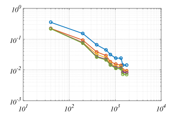
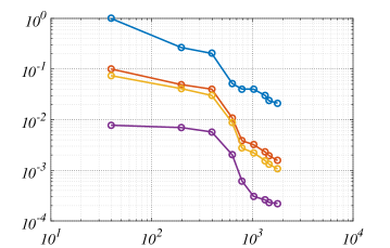
Figure 1: Log-Log plots of errors in the energy norm vs. first eigenvalue out of the expansion after applying GMsFEM to Examples $1$ and $2$. (Left) source term and exact solution in (34). (Right) source term and exact solution in (35). Each color correspond to a fixed $N_{D}=\{0,5,10,15,20\}$ and ($N_{D}=\{0,1,2,3\}$ (right)) and each circle correspond to $N_{N}=\{1,5,10,...,40\}$.

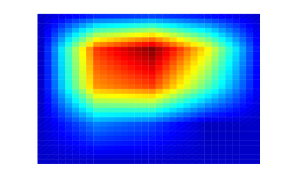
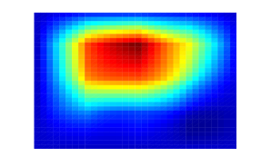
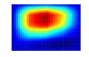
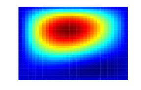
Figure 2: Level plots of $3$ approximations of exact solution $u_{1}$ in (34). (Up-Left 2-$N_{N}$, 2-$N_{D}$), (Up-Right 3-$N_{N}$, 3-$N_{D}$) and (Down-Left 4-$N_{N}$, 4-$N_{D}$) evolving to exact solution (Down-Right).

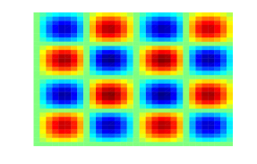
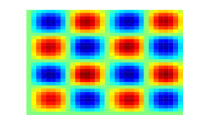
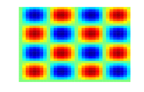
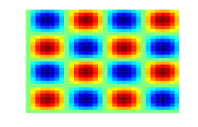
Figure 3: Level plots of $3$ approximations of exact solution $u_{2}$ in (35). (Up-Left 1-$N_{N}$, 0-$N_{D}$), (Up-Right 2-$N_{N}$, 0-$N_{D}$) and (Down-Left 3-$N_{N}$, 0-$N_{D}$) evolving to exact solution (Down-Right).

In the first example, including Dirichlet functions doesn’t have much impact in the approximation, the error in the energy norm decreases faster by including more Newmann functions. While in the second example by including Dirichlet functions the energy norm decreases faster than by including Newman functions as we can see in Figure 1

Now let us consider two different heterogeneous fields. The first is shown is composed by 3 chanels of high permeability in $64\times 64$ fictitious geological mesh shown in Figure 4. The second heterogeneous medium to be consider will be the last $64\times 64$ block of the geological permeability $SPE10$ porous medium taken from [32] (see Figure 5). This is a widely used heterogeneous porous medium for simulations (see for example [33])

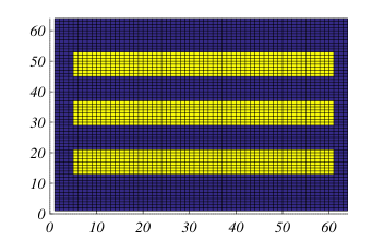
Figure 4: Heterogenous high permeability $3$-channels medium in a $64\times 64$ mesh.

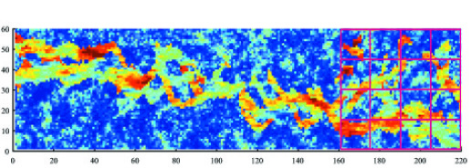
Figure 5: A 2D layer of the $SPE10$ 2D porous medium sample from [32].

Next we perform two numerical experiments to evaluate the performance of including Dirichlet basis when heterogeneity of the medium is present.

Experiment $3$: Let us consider a source taking alternating values $1$ and $-1$ on the $4\times 4$ coarse mesh $\mathcal{T}^{H}$ of $\Omega$

$$f_{3}(x,y)=\begin{cases}1&if\leavevmode\nobreak\ \leavevmode\nobreak\ (x,y)\in K_{2j}\\ -1&if\leavevmode\nobreak\ \leavevmode\nobreak\ (x,y)\in K_{2j-1}\end{cases}$$ (36)

with $K_{j}\in\mathcal{T}^{H}$ and $j\in\{1,..,16\}$. The coarse mesh basis are computed on the fine $512\times 512$ mesh $\mathcal{T}^{h}$ and approximated reference solution is computed in a $1024\times 1024$ finner mesh using classical finite element $\mathcal{Q}^{1}$. As we did in Examples $1$ and $2$ we fix the number of Dirichlet coarse basis in the expansion $N_{D}$ from $1$ to $20$ and vary the number of Newmann coarse basis $N_{N}$ from $1$ to $40$. We use the $3$-channels heterogeneous medium shown in Figure 4

Experiment $4$: Exactly the same parameters in Experiment $3$ except for the medium which will be taken from SPE10 as previously described and shown in Figure 5.

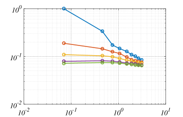
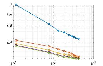
Figure 6: Log-Log plots of errors in the energy norm Vs. first eigenvalue out of the expansion after applying GMsFEM to Experiments $3$ and $4$ using source term in (36).(Left) Heterogenous $3-chanels$ medium (Figure 4). (Right) heterogeneous $SPE10$ medium (Figure 5). Each color correspond to a fixed $N_{D}=\{0,5,10,15,20\}$ and each circle correspond to $N_{N}=\{1,5,10,...,40\}$.

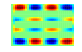
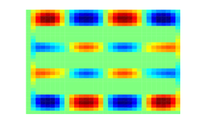
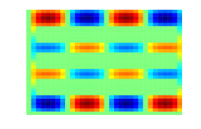
Figure 7: Level plots of $3$ approximations of solution of Experiment $3$ (Up-Left 1-$N_{N}$, 0-$N_{D}$), (Up-Right 5-$N_{N}$, 0-$N_{D}$) and (Down-Left 10-$N_{N}$, 0-$N_{D}$) evolving to reference solution (Down-Right) computed in a finner mesh $1024\times 1024$.

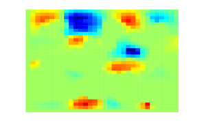
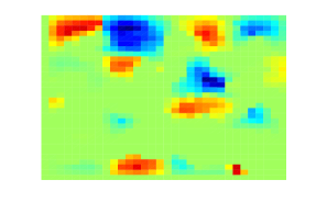
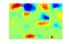
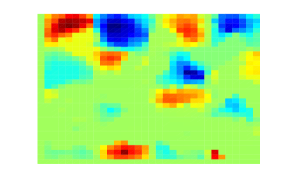
Figure 8: Level plots of $3$ approximations of solution of Experiment $4$. (Up-Left 40-$N_{N}$, 0-$N_{D}$), (Up-Right 10-$N_{N}$, 5-$N_{D}$) and (Down-Left 40-$N_{N}$, 20-$N_{D}$) evolving to reference solution (Down-Right) computed in a finner mesh $1024\times 1024$.

Both for Experiment $3$ and $4$ the approximated solution benefits from including Dirichlet basis in the expansion.

10 Discussions and final comments

In this paper, we obtained error estimates for GMsFEM approximation of high-contrast multiscale problems. This construction uses local Neumann eigenvectors on neighborhoods and Dirichlet eigenvectors on elements to construct finite element basis function. The analysis is based on eigenfunction expansions and the norms used for the error estimates measure the decay of the expansion of the solution in terms of local eigenfunctions. The norms in the interpolation error estimates can be bounded by the $L^{2}$ norm of a rescaling of the forcing term. For the analysis we assume that the solution can be approximated by a sum of two functions, one with zero flux across coarse blocks boundaries, and the other with zero value on coarse blocks boundaries. This assumption is easily verified for classical regular problems. The introduction of this assumption allowed us to extend and simplify the convergence analysis presented in [22]. The error estimates derived here can be applied to several situations that are under current research. For instance, it is possible to obtain error estimates for general bilinear forms using the analysis presented here combined with the construction of coarse spaces in [34].

Notation

In general we use the letters $\mu$ and $\phi$ to refer to Dirichlet eigenvalues and eigenvectors; and we use letters $\lambda$ and $\psi$ to refer to Newmann eigenvalues and eigenvectors. Letter $\Phi$ is reserved to generalized basis.

Table 1: Table of Notation

$\Omega$	pag.4	Definition domain of the elliptic problem
$H^{1}(\Omega)$	pag.9	Sobolev space of functions with continuous first derivatives on $\Omega$
$H_{0}^{1}(\Omega)$	pag.4	Sobolev space of functions with continuous first derivatives on $\Omega$ and vanishing on $\partial\Omega$
$w_{i}$	pag.5	Neighborhood of the node $y_{i}$ of a triangulation.
$w^{K}$	pag.5	Union of all neighborhood containing the element $K$
$\mu^{K}_{l}$	pag.10	$l-th$ Dirichlet eigenvalue of the local eigenvalue problem on $K$
$\phi^{K}_{l}$	pag.10	$l-th$ Dirichlet eigenfunction of the local eigenvalue problem on $K$.
$\lambda^{w_{i}}_{l}$	pag.12	$l-th$ Newmann eigenvalue of the local eigenvalue problem on $w_{i}$.
$\psi^{w_{i}}_{l}$	pag.12	$l-th$ Newmann eigenfunction of the local eigenvalue problem on $w_{i}$.
$\Phi_{i}$	pag.12	Generalased basis function associated to the neighborhood $w_{i}$
$\mathcal{A}$	pag.7	Elliptic operator on $\Omega$.
$\mathcal{A}^{K}$	pag.11	Elliptic operator on the coarse block $K$.
$\mathcal{A}^{w_{i}}$	pag.13	elliptic operator defined on the neighborhood $w_{i}$.
$\mathcal{J}_{L}$	pag.9	Dirichlet projection operator truncated at $L$.
$\mathcal{J}_{L}^{K}$	pag.13	Dirichlet projection operator on element $K$ truncated at $L$.
$I^{\omega_{i}}_{L}$	pag.18	Newmann projection operator in on neighborhood $\omega_{i}$ truncated at $L$.
$I_{N}$	pag.19	Generalized basis coarse interpolation operator
$J_{D}$	pag.19	Dirichlet basis coarse interpolation operator
$\widetilde{V}(\omega_{i})$	pag.12	Space of functions in $H^{1}(w_{i})$ which are zero on $\partial w_{i}\cap\partial\Omega$.
$|||v|||_{s;{D}}$	pag.6	Norms based on the eigenvalue expansion decay on an set $D$.

References

References

- [1] T. Hou, X. Wu, A multiscale finite element method for elliptic problems in composite materials and porous media, J. Comput. Phys. 134 (1997) 169–189.
- [2] J. Aarnes, T. Hou, Multiscale domain decomposition methods for elliptic problems with high aspect ratios, Acta Math. Appl. Sin. Engl. Ser. 18 (2002) 63–76.
- [3] J. Aarnes, Y. Efendiev, L. Jiang, Analysis of multiscale finite element methods using global information for two-phase flow simulations, SIAM J. Multiscale Modeling and Simulation 7 (2008) 2177–2193.
- [4] L. Berlyand, H. Owhadi, A new approach to homogenization with arbitrary rough high contrast coeffcients for scalar and vectorial problems, Submitted.
- [5] J. Aarnes, S. Krogstad, K.-A. Lie, A hierarchical multiscale method for two-phase flow based upon mixed finite elements and nonuniform grids, SIAM J. Multiscale Modeling and Simulation 5 (2) (2006) 337–363.
- [6] T. Arbogast, Implementation of a locally conservative numerical subgrid upscaling scheme for two-phase Darcy flow, Comput. Geosci 6 (2002) 453–481.
- [7] T. Arbogast, G. Pencheva, M. Wheeler, I. Yotov, A multiscale mortar mixed finite element method, SIAM J. Multiscale Modeling and Simulation 6 (1) (2007) 319–346.
- [8] Y. Chen, L. Durlofsky, M. Gerritsen, X. Wen, A coupled local-global upscaling approach for simulating flow in highly heterogeneous formations, Advances in Water Resources 26 (2003) 1041–1060.
- [9] Y. Efendiev, V. Ginting, T. Hou, R. Ewing, Accurate multiscale finite element methods for two-phase flow simulations, Journal of Computational Physics 220 (2006) 155–174.
- [10] P. Jenny, S. Lee, H. Tchelepi, Multi-scale finite volume method for elliptic problems in subsurface flow simulation, J. Comput. Phys. 187 (2003) 47–67.
- [11] C. Chu, I. Graham, T. Hou, A new multiscale finite element methods for high-contrast elliptic interface problem, Mathematics of Computation 79 (2010) 1915–1955.
- [12] T. Hughes, G. Feijoo, L. Mazzei, J. Quincy, The variational multiscale method - a paradigm for computational mechanics, Comput. Methods Appl. Mech. Engrg. 166 (1998) 3–24.
- [13] Y. Efendiev, T. Hou, Multiscale Finite Element Methods: Theory and Applications, Vol. 4 of Surveys and Tutorials in the Applied Mathematical Sciences, Springer, New York, 2009.
- [14] J. Galvis, Y. Efendiev, Domain decomposition preconditioners for multiscale flows in high contrast media, SIAM J. Multiscale Modeling and Simulation 8 (2010) 1461–1483.
- [15] J. Galvis, Y. Efendiev, Domain decomposition preconditioners for multiscale flows in high contrast media. reduced dimension coarse spaces, SIAM J. Multiscale Modeling and Simulation 8 (2010) 1621–1644.
-
[16]
E. Burman, J. Guzmán, M. A. Sánchez, M. Sarkis,
Robust flux error estimation of
an unfitted Nitsche method for high-contrast interface problems, IMA J.
Numer. Anal. 38 (2) (2018) 646–668.
doi:10.1093/imanum/drx017.
URL https://doi.org/10.1093/imanum/drx017 -
[17]
E. Burman, J. Guzmán, M. A. Sánchez, M. Sarkis,
Robust flux error estimation of
an unfitted Nitsche method for high-contrast interface problems, IMA J.
Numer. Anal. 38 (2) (2018) 646–668.
doi:10.1093/imanum/drx017.
URL https://doi.org/10.1093/imanum/drx017 -
[18]
E. T. Chung, Y. Efendiev, W. T. Leung,
An adaptive generalized multiscale
discontinuous Galerkin method for high-contrast flow problems, Multiscale
Model. Simul. 16 (3) (2018) 1227–1257.
doi:10.1137/140986189.
URL https://doi.org/10.1137/140986189 - [19] Y. Efendiev, T. Hou, V. Ginting, Multiscale finite element methods for nonlinear problems and their applications, Comm. Math. Sci. 2 (2004) 553–589.
- [20] Y. Efendiev, T. Hou, X. Wu, Convergence of a nonconforming multiscale finite element method, SIAM J. Numer. Anal. 37 (2000) 888–910.
- [21] Y. Efendiev, J. Galvis, R. Lazarov, J. Willems, Robust domain decomposition preconditioners for abstract symmetric positive definite bilinear forms, ESIAM : M2AN 46 (2012) 1175–1199.
- [22] Y. Efendiev, J. Galvis, X. Wu, Multiscale finite element methods for high-contrast problems using local spectral basis functions, Journal of Computational Physics 230 (2011) 937–955.
-
[23]
V. M. Calo, Y. Efendiev, J. Galvis,
Asymptotic expansions for
high-contrast elliptic equations, Math. Models Methods Appl. Sci. 24 (3)
(2014) 465–494.
doi:10.1142/S0218202513500565.
URL http://dx.doi.org/10.1142/S0218202513500565 - [24] Y. Efendiev, J. Galvis, E. Gildin, Local-global multiscale model reduction for flows in highly heterogeneous media, Submitted.
- [25] Y. Efendiev, J. Galvis, Coarse-grid multiscale model reduction techniques for flows in heterogeneous media and applications, Chapter of Numerical Analysis of Multiscale Problems, Lecture Notes in Computational Science and Engineering, Vol. 83. 97–125.
- [26] Y. Efendiev, J. Galvis, T. Hou, Generalized multiscale finite element methods, Journal of Computational Physics 251 (2013) 116–135.
- [27] Y. Efendiev, J. Galvis, F. Thomines, A systematic coarse-scale model reduction technique for parameter-dependent flows in highly heterogeneous media and its applications, Multiscale Model. Simul. 10 (2012) 1317–1343.
- [28] Y. Efendiev, J. Galvis, Domain decomposition preconditioner for multiscale high-contrast problems, in: Proceedings of DD19, 2009.
-
[29]
Y. Efendiev, J. Galvis, R. Lazarov, J. Willems,
Robust domain decomposition
preconditioners for abstract symmetric positive definite bilinear forms,
ESAIM Math. Model. Numer. Anal. 46 (5) (2012) 1175–1199.
doi:10.1051/m2an/2011073.
URL http://dx.doi.org/10.1051/m2an/2011073 - [30] I. Babuška, V. Nistor, N. Tarfulea, Generalized finite element method for second-order elliptic operators with Dirichlet boundary conditions, J. Comput. Appl. Math. 218 (2008) 175–183.
- [31] K. C. T. Strouboulis, I. Babuška, The design and analysis of the generalized finite element method, Comput. Methods Appl. Mech. Engrg. 181 (2000) 43–69.
- [32] S. of petrleum ingeneers, Spe comparative solution project, https://www.spe.org/web/csp/.
-
[33]
M. Christie, M. Blunt, Tenth spe
comparative solution project: A comparison of upscaling techniques, Society
of Petroleum Engineersdoi:10.2118/72469-PA.
URL https://doi.org/10.2118/72469-PA - [34] Y. Efendiev, J. Galvis, R. Lazarov, J. Willems, Robust domain decomposition preconditioners for abstract symmetric positive definite bilinear forms, ESAIM: Mathematical Modelling and Numerical Analysis (2012) 1175–1199.