Jarzynski equality for superconducting optical cavities: an alternative path to determine Helmholtz free energy

Abstract

A superconducting cavity model was proposed as a way to experimentally investigate the work performed in a quantum system. We found a simple mathematical relation between the free energy variation and visibility measurement in quantum cavity context. If we consider the difference of Hamiltonian at time $t_{0}$ and $t_{\lambda}$ (protocol time) as a quantum work, then the Jarzynski equality is valid and the visibility can be used to determine the work done on the cavity.

1 Introduction

Fluctuation theorems have been developed to describe systems far from equilibrium, that is the case of Jarzynski equality (JE) [1, 2, 3, 4] and Crooks relation [5] and Bochkov-Kuzovlev [6]. The classical JE is a relation between the free energy difference of two equilibrium states ($\Delta F$) and the work ($W$) averaged over all possible paths of a nonequilibrium process linking them. Mathematically the JE is

$$e^{-\beta\Delta F}=\langle e^{-\beta W}\rangle.$$ (1)

The JE was developed assuming that the system is isolated from the reservoir while the protocol is performed. Morgado and Pinto [7] have obtained JE for a massive Brownian particle connected to internal and external springs, their result does not depend on the decoupling of system and bath along the protocol time, a Brownian particle was also experimentally investigated in context of JE [8]. Minh and Adib [9] have used path integral formalism and demonstrated that the validity of JE in the context of Brownian particle subject a class of harmonic potential.

Experimentally some important results were achieved, Liphardt and collaborators [10] demonstrated the validity of JE by mechanically stretching a single molecule of RNA reversibly and irreversibly between two conformations. Toyabe and collaborators [2] have investigated experimentally the JE for a dimeric particle comprising polystyrene beads by attaching it to a glass surface of a chamber filled with a buffer solution, they have found a discrepancy smaller than $3\%$ between the observed result and what was expected with JE. Douarche and collaborators [11] have experimentally checked the Jarzynski equality and the Crooks [5] relation on the thermal fluctuations of a macroscopic mechanical oscillator in contact with a heat reservoir and found a good agreement with JE and crooks relation. Hoang et al. [12] have performed an experimental test of JE and Hummer-Szabo relation [13] using an optically levitated nanosphere. These, among many others experimental investigation consolidates the JE in the classical domain

In this work, we use the quantum analog of Jarzynski equality (JE) to propose a way to obtain experimentally the work performed in a quantum system. The Quantum version of (JE) is a controversy area, the first attempts to derive Jarzynski equalities for quantum systems failed [6, 15, 14] leading to misleadingly believed that the equality was not valid for quantum systems. In some of this earlier derivations of Jarzynski equation for quantum systems a work operator was defined [6, 14, 15, 16, 17], but this work definition is not, in general, a quantum observable [18] this is due to the fact that work characterize a process rather than an instantaneous state of the system. This earlier attempts had led to quantum corrections to the classical Jarzynski result and the classical result was recovered only when the Hamiltonian in a time $t$ commutes with itself in a time $t^{\prime}$ [16].

Recently the discussion has been changed to how to define operational ways of measuring work since Jarzynski’s equality has already been obtained for closed quantum systems [25, 26, 18, 19, 22] for open systems [27, 5, 23] even for systems with strong couplings [24]. Most of these proposals are linked to the question of measuring energy in two moments, which from a quantum point of view introduce several questions since a quantum systems have a dynamical behavior that is affected by the measurements, thus since one performs energy measurements the system state changes, this problem is circumvented if one use non-demolition measurements, in reference [28] they show that POVM (positive operator valued measure) can be used to sample the work probability distribution. Experimentally, some advances have been achieved, An and collaborators [29] have investigated experimentally the JE in the quantum domain. They have used ${}^{171}Yb_{+}$ ion trapped in a harmonic potential and perform projective measurements to obtain phonon distributions of the initial thermal state, they have concluded that JE still valid, a similar result was obtained by measuring a single-molecule [30].

In this work, we study a transition between two equilibrium states of a quantum system, namely a quantum harmonic oscillator coupled to a thermal bath. This model can be implemented with a cavity quantum electrodynamics (CQED) [31]. The protocol can be executed by injecting a coherent field in the cavity. The CQED experimental setup was widely used to explore quantum mechanical foundations with many interesting results (see [32, 33, 34, 35] and references therein). Even for a more realistic model [36], that consider environment action, the quantum nature of the electromagnetic field was demonstrated. Experimentally, the initial state was prepared in a pure state [34], usually in a vacuum. We consider a thermal state, as the initial state, and the work is given by the difference of cavity’s Hamiltonian $\Delta H=H(\tau)-H(0)$ where $\tau$ is a time bigger than the protocol time. The thermal state is not a guarantee of a “classical state” [38], but surprisingly, for the work as defined above, the JE is valid in all quantum domain [28, 18, 20, 21]. Cerisola and collaborators [39] have shown that JE is valid in quantum domain for a more general measurement class named “a quantum work meter”. Assuming that JE is valid, we show that the free energy variation and also the mean $\langle e^{-\beta W}\rangle$ can be simply inferred by a measurement of fringes visibility in the context of CQED.

2 Quantum Jarzynski Equality

We consider a Quantum analog of the model studied by [40]. It consists of $N$ non-interacting harmonic oscillators all initially in thermal equilibrium at temperature $T$, then the partition function is

$$Z(0)=\prod_{n=1}^{N}Z_{n}(0)$$ (2)

with

$$Z_{n}(0)=\frac{\exp\left(-\frac{1}{2}\beta\hbar\omega_{0}\right)}{1-\exp\left(-\beta\hbar\omega_{0}\right)}.$$ (3)

After the action of the protocol, the equivalent quantum Hamiltonian of $n$th oscillator for $t^{\prime}<t$ is

$$\hat{H}_{n}(t^{\prime})=\frac{\hat{p}_{n}^{2}}{2m}+\frac{1}{2}m\omega_{0}^{2}\hat{x}_{n}^{2}+l\hat{x}_{n}L\left(t^{\prime}\right).$$ (4)

Then its eigenvectors are the same of harmonic oscillator and the energies are

$$E_{n}(t^{\prime})=\left(j+\frac{1}{2}\right)\hbar\omega_{0}-\frac{1}{2}\frac{l^{2}L^{2}(t^{\prime})}{m\omega_{0}^{2}},$$ (5)

where $j$ are positive integers. Thus the partition function reads

$$Z(t^{\prime})=\prod_{n=1}^{N}Z_{n}(t^{\prime}),$$ (6)

with

$$Z_{n}(t^{\prime})=\exp\left[\frac{\beta l^{2}L^{2}(t^{\prime})}{2m\omega_{0}^{2}}\right]\left[\frac{\exp\left(-\frac{1}{2}\beta\hbar\omega_{0}\right)}{1-\exp\left(-\beta\hbar\omega_{0}\right)}\right],$$

and Helmholtz free energy to the $n$-th oscillator of the system is

$$F_{n}=\dfrac{\hbar\omega_{0}}{2}-\dfrac{l^{2}L^{2}(t^{\prime})}{2m\omega_{0}}+\dfrac{1}{\beta}\ln\left[1-\exp\left(-\beta\hbar\omega_{0}\right)\right].$$ (7)

Again, the protocol changes $L$ parameter from $L_{0}$ to $L_{1}$. Thus,

$$\Delta F_{n}=\frac{l^{2}}{2m\omega_{0}^{2}}\left(L_{0}^{2}-L_{1}^{2}\right).$$ (8)

It is easy to see that the variation of the Helmholtz free energy to the system will be

$$\Delta F=\sum_{n=1}^{N}\Delta F_{n}.$$ (9)

Since we are dealing with $N$ non-interacting harmonic oscillators, without loss of generality, we can restrict our analysis to a single oscillator of system. We will do this from now on.

2.1 Quantum work

The Hamiltonian ($\hat{H}(t^{\prime})$) to a single oscillator of system is

$$\hat{H}_{n}(t^{\prime})=\frac{\hat{p_{n}}^{2}}{2}+\frac{\omega_{0}^{2}}{2}\left[\hat{x_{n}}^{2}+\frac{2l\hat{x_{n}}L(t^{\prime})}{\omega_{0}^{2}}\right].$$ (10)

where we set $m=\hbar=1$. We can also write the Hamiltonian in terms of creation and annihilation operators, and it will be useful in the next sections, it is given by

$$\hat{H}_{n}(t^{\prime})=\omega_{0}\left(\hat{a_{n}}^{\dagger}\hat{a_{n}}+\frac{1}{2}\right)+\tilde{L}(t^{\prime})\left(\hat{a}+\hat{a}^{\dagger}\right).$$ (11)

where $\tilde{L}(t^{\prime})=\sqrt{\frac{\hbar}{2m\omega_{0}}}L(t^{\prime})$.

We assume that the system environment coupling is not relevant during the protocol time, if we assume that the necessary work [40] to change $L_{0}\longmapsto L_{1}$ is the same as the system energy variation $\Delta E$, then at $t=0$ we find an energy $E_{n}^{(0)}$ with a probability given by

$$P_{n}^{(0)}=\frac{\exp\left(-\beta E_{n}^{(0)}\right)}{Z}\text{ .}$$ (12)

After a time $t_{f}$ the system is in a state $\hat{U}(t_{f})\left|\psi_{n}^{0}\right\rangle$ and the transition probability is

$$w_{mn}=\left|\left\langle\psi_{m}^{(f)}\right|\hat{U}(t_{f})\left|\psi_{n}^{(0)}\right\rangle\right|^{2}.$$ (13)

Here, $\hat{U}(t_{f})$ is

$$\hat{U_{n}}(t_{f})=T_{>}\exp\left[-\frac{i}{\hbar}\int_{0}^{t_{f}}dt^{\prime}\hat{H}_{n}(t^{\prime})\right],$$ (14)

where $T_{>}$ denotes time ordering operator. Finally, we obtain

$$\left\langle\exp(-\beta\Delta E)\right\rangle=\underset{n}{\sum}P_{n}^{(0)}\underset{m}{\sum}w_{mn}\exp(-\beta\Delta E)$$ (15)

with $\Delta E=E_{m}^{\left(f\right)}-E_{n}^{\left(0\right)}$. After some manipulations [40] we get

$$\left\langle\exp(-\beta\Delta E)\right\rangle=\exp\left[\frac{N\beta l^{2}}{2\omega_{0}^{2}}\left(L_{1}^{2}-L_{0}^{2}\right)\right].$$ (16)

Comparing (16) with (8) its clear that JE is verified, what was expected (see Ref. [16]).

3 Visibility of Interference Fringes and its connection with JE

In this section, we verify the possibility of an experimental realization procedure. We assume that the harmonic oscillator is a microwave field stored in a high-$Q$ superconducting cavity. The field state can be monitored by establishing an interaction with a Rydberg atom [31, 35, 41]. Rydberg atoms have suitable properties for use as probes of even weak electromagnetic fields, such as high dipole moments, which ensure high coupling strengths, and high mean lifetimes. We consider a non-demolition measurement procedure [42] of the number of photons contained in the electromagnetic field by setting a dispersive interaction between it and each Rydberg atom. The number of photons in the cavity is probed by Ramsey interferometry [43], and this measure allows obtaining some information about the field state inside the cavity.

A schematic representation of the experimental setup is illustrated in FIG. 1.

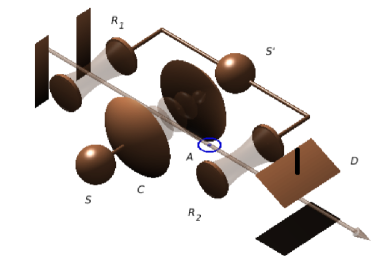
Figure 1: Schematic representation of the apparatus used in a typical Ramsey interferometry with Rydberg atoms. A Rydberg atom $A$, in general, an atom of an alkali element, is prepared a highly excited electronic level $\left|g\right\rangle$ and it is sent through the apparatus. The two Ramsey zones, $R_{1}$ and $R_{2}$, are low-$Q$ cavities devised to change the atomic states as $\left|g\right\rangle\rightarrow\left(\left|g\right\rangle+\left|f\right\rangle\right)/\sqrt{2}$ and $\left|f\right\rangle\rightarrow\left(-\left|g\right\rangle+\left|f\right\rangle\right)/\sqrt{2}$. Despite the low mean number of photons inside the two Ramsey zones, from the practical point of view, the atom sees a classical field there, so much that the atom leaves the Ramsey zones in a non-entangled state. In the superconducting microwave cavity $C$ the atom interacts dispersively with the cavity field. This interaction glues different phase shifts in each atomic state that depends on the number of photons of the cavity field. So, right after the atom leaves the superconducting cavity $C$, the global state of atom plus the field inside it remains entangled. The detector $D$ measures the atom at $\left|f\right\rangle$. Repeating the process under slight different conditions (for example, changing the frequency of the mode inside the Ramsey zones) a interferometric pattern is produced, and the information about the number of photons of the mode inside the cavity $C$ can be extracted.

We consider a three-level Rydberg atom, as illustrated in Fig. 2.

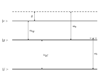
Figure 2: Three-level atom. The states $|e\rangle$ and $|f\rangle$ have the same parity and are opposed to the parity of $|g\rangle$. The field in the superconducting cavity has frequency $\omega_{0}$ and is de-tuned of $\delta=\omega_{0}-\omega_{eg}$ from transition frequency $\omega_{eg}=(E_{e}-E_{g})/\hbar$ between levels $|e\rangle$ and $|g\rangle$. The Ramsey zones [43] have frequencies $\omega_{r}$ and are close to the transition transition sintony frequency $\omega_{gf}=(E_{g}-E_{f})/\hbar$ between levels $|g\rangle$ and $|f\rangle$.

The three-level atom is sent through an apparatus as schematized in FIG. 1. The atom, when passing through $C$, will interact dispersively with the atom inside it and the interest Hamiltonian is

$$\hat{H}=\hbar\omega_{0}\biggl{(}\hat{a}^{\dagger}\hat{a}+\frac{1}{2}\biggr{)}+E_{e}|e\rangle\langle e|+E_{g}|g\rangle\langle g|+E_{f}|f\rangle\langle f|+\hbar\omega\Bigl{[}\bigl{(}\hat{a}^{\dagger}\hat{a}+1\bigr{)}|e\rangle\langle e|-\hat{a}^{\dagger}\hat{a}|g\rangle\langle g|\Bigr{]},$$ (17)

where $\hat{a}^{\dagger}$ ($\hat{a}$) is the creation (annihilation) operator acting on the field state inside the cavity $C$, $|i\rangle$ is the $i$-th atomic level, defined as $i=e$, $g$ and $f$, $E_{i}$ is the corresponding energy of the $i$th level and $\omega_{0}$ is the field frequency in $C$, $\omega=\Omega_{0}^{2}/4\delta$ is the coupling constant in the dispersive regime, $\Omega_{0}$ is the vacuum Rabi frequency inside cavity $C$ and $\delta$ is the atom-field detuning between transition frequency of the energy levels $|e\rangle$ and $|g\rangle$, $\omega_{eg}=(E_{e}-E_{g})/\hbar$, and the frequency of the stored mode in $C$, $\omega_{0}$.

Without lost of generality, equation (17) can be presented as

$$\hat{H}=\hat{H}_{0}+\hat{H}_{I},$$ (18)

where

$$\hat{H}_{0} = \hbar\omega_{0}\biggl{(}\hat{a}^{\dagger}\hat{a}+\frac{1}{2}\biggr{)}+(E_{e}+\hbar\omega)|e\rangle\langle e|+E_{g}|g\rangle\langle g|+E_{f}|f\rangle\langle f|,$$ (19)

$$\hat{H}_{I} = \hbar\omega\,\hat{a}^{\dagger}\hat{a}\,\bigl{(}|e\rangle\langle e|-|g\rangle\langle g|\bigr{)}.$$ (20)

We observe that $[\hat{H}_{0},\hat{H}_{I}]=0$, then, in the interaction picture we have an arbitrary state of the field in cavity $C$, it is given by

$$\rho_{F}(0)=\sum_{i,j}\rho_{i,j}|i\rangle\langle j|,$$ (21)

an atom is sent to interact with the field in cavity $C$, this atom is previously prepared in the state

$$\rho_{A}(0)=g|g\rangle\langle g|+f|f\rangle\langle f|+\bigl{[}\,x|g\rangle\langle f|+c.h.\bigr{]},$$ (22)

with $g+f=1$ and $|x|^{2}\leq gf$. After a time interval $\Delta t$, the atom-field state in the interaction picture, is given by

$$\rho(\Delta t)=e^{-iH_{I}\Delta t/\hbar}\rho_{F}(0)\rho_{A}(0)e^{iH_{I}\Delta t/\hbar}$$ (23)

taking the trace in field variables in time $\Delta t$ we obtain the atomic state that is

$$\rho_{A}(\Delta t)=\mathrm{Tr}_{F}\bigl{[}\rho(\Delta t)\bigr{]}.$$ (24)

As the atom goes through $R_{2}$ the states $|g\rangle$ and $|f\rangle$ will be entangled with a relative phase $\phi$, as we can observe in FIG. 1. After that, the atom is measured in $D$ and as we change $\phi$, the Ramsey interference fringes appear. The visibility $\mathcal{V}$ of the interference fringes pattern is proportional to the absolute value of coherence’s term of the state (24) and can be obtained by

$$\mathcal{V}(\Delta t)=2\Bigl{|}\mathrm{Tr}\bigl{[}\rho_{A}(\Delta t)|g\rangle\langle f|\bigr{]}\Bigr{|},$$ (25)

as we can see in reference [44].

The visibility $\mathcal{V}$ depends on field state eq.(21), then the interference fringes carries field state information, it becomes clear as we analyze equation (24) in deeper, we have:

$$\rho_{A}(\Delta t) = \sum_{m}\langle m|e^{-iH_{I}\Delta t/\hbar}\rho_{F}(0)\rho_{A}(0)e^{iH_{I}\Delta t/\hbar}|m\rangle$$ (26)

$$= \sum_{m}\langle m|e^{-iH_{I}\Delta t/\hbar}\rho_{F}(0)e^{iH_{I}\Delta t/\hbar}e^{-iH_{I}\Delta t/\hbar}\rho_{A}(0)e^{iH_{I}\Delta t/\hbar}|m\rangle$$

$$= \sum_{m,n}\langle m|e^{-iH_{I}\Delta t/\hbar}\rho_{F}(0)e^{iH_{I}\Delta t/\hbar}|n\rangle\langle n|e^{-iH_{I}\Delta t/\hbar}\rho_{A}(0)e^{iH_{I}\Delta t/\hbar}|m\rangle.$$

Taking (21) into (26), we obtain

$$\rho_{A}(\Delta t) = \sum_{m,n}\rho_{m,n}e^{-i\omega\Delta t(m-n)\bigl{(}|e\rangle\langle e|-|g\rangle\langle g|\bigr{)}}\delta_{n,m}e^{-i\omega\Delta t(n-m)|e\rangle\langle e|}e^{i\omega\Delta tn|g\rangle\langle g|}\rho_{A}(0)e^{-i\omega\Delta tm|g\rangle\langle g|}$$ (27)

$$= \sum_{n,n}\rho_{n,n}e^{i\omega\Delta tn|g\rangle\langle g|}\rho_{A}(0)e^{-i\omega\Delta tn|g\rangle\langle g|}$$

$$= g|g\rangle\langle g|+f|f\rangle\langle f|+\bigl{[}\,x\sum_{n}\rho_{n,n}e^{in\omega\Delta t}|g\rangle\langle f|+c.h.\bigr{]}.$$

We observe that the term $\sum_{n}\rho_{n,n}e^{in\omega\Delta t}$ in the equation (27) can be written as

$$\sum_{n}\rho_{n,n}e^{in\omega\Delta t} = \sum_{n}\langle n|\rho_{F}(0)e^{i\omega\Delta ta^{\dagger}a}|n\rangle$$ (28)

$$= \mathrm{Tr}\Bigl{[}\rho_{F}(0)e^{i\omega\Delta ta^{\dagger}a}\Bigr{]}.$$

Now, introducing (28) into 27) the field state is given by

$$\rho_{A}(0)=g|g\rangle\langle g|+f|f\rangle\langle f|+\bigl{[}\,\bar{x}|g\rangle\langle f|+c.h.\bigr{]},$$ (29)

where $\bar{x}=x\,\mathrm{Tr}\Bigl{[}\rho_{F}(0)e^{i\omega\Delta ta^{\dagger}a}\Bigr{]}$. We can obtain the Ramsey interference fringes visibility, equation (25) for the atom in the state(29), then

$$\mathcal{V}(\Delta t)=\mathcal{V}_{0}\biggl{|}\mathrm{Tr}\Bigl{[}\rho_{F}(0)e^{i\omega\Delta ta^{\dagger}a}\Bigr{]}\biggr{|}.$$ (30)

The visibility clearly depends on field initial state. In equantion (30) we defined $\mathcal{V}_{0}=2|x|$, it is the visibility of the vacuum state. Form now on, we consider the optimum case where$\mathcal{V}_{0}=1$. This occurs when $|x|=1/2$ and the atom state is $(|g\rangle+e^{i\theta}|f\rangle)/\sqrt{2}$, and $\theta$ is a arbitrary relative phase.

3.1 The field state in a equilibrium Thermal State

Following the previous mathematical procedure, easily we can obtain the visibility when we have in $C$ a field initially in a thermal given by

$$\rho_{Th}=\frac{e^{-\beta\bar{H}}}{Z},$$ (31)

where $\bar{H}=\hbar\omega_{0}\bigl{(}a^{\dagger}a+1/2\bigr{)}$ is the field Hamiltonian that is in thermal equilibrium and $Z=\mathrm{Tr}\bigl{(}e^{-\beta\bar{H}}\bigr{)}$ , as usual, is the partition function. Then, after some algebra we obtain

$$\mathcal{V}_{Th}(\Delta t)=\dfrac{\sinh(\beta\hbar\omega_{0}/2)}{\sqrt{\sinh^{2}(\beta\hbar\omega_{0}/2)+\sin^{2}(\omega\Delta t/2)}}.$$ (32)

For practical proposes, the perfect choice of the interaction time can be obtained if we adopt $\omega\Delta t=\pi$, then equation(32) can now be written as

$$\mathcal{V}_{Th}(\pi/\omega)=\tanh(\beta\hbar\omega_{0}/2).$$ (33)

It is interesting to note that equation (32) can be simplified in two limiting cases

$$\mathcal{V}_{Th}(\pi/\omega)\approx\left\{\begin{array}[]{rcc}\beta\hbar\omega_{0}/2,&\mathrm{se}&\beta\hbar\omega_{0}\ll 1,\\ &&\\ 1,&\mathrm{se}&\beta\hbar\omega_{0}\gg 1.\end{array}\right.$$ (34)

3.2 The field state in a Displaced Thermal State

The Hamiltonian for a displaced field in a cavity $C$ is given by

$$\tilde{H}=\hbar\omega_{0}\Bigl{(}a^{\dagger}a+\frac{1}{2}\Bigr{)}+\hbar\omega_{0}\bigl{(}\alpha a^{\dagger}+\alpha^{*}a\bigr{)}.$$ (35)

where $\alpha$ is the displacement magnitude, observe that it is directly related with the protocol term $\tilde{L}$ in equation (11). The Hamiltonian (35) can be written as

$$\tilde{H}=D^{{\dagger}}(\alpha)\bar{H}D(\alpha)-\hbar\omega_{0}|\alpha|^{2},$$ (36)

where $D$ is the displacement operator defined as $D(\alpha)=\exp\bigl{(}\alpha a^{\dagger}-\alpha^{*}a\bigr{)}$. In this case, the thermal equilibrium state is

$$\rho^{(\alpha)}_{Th}=\frac{e^{-\beta\tilde{H}}}{Z^{(\alpha)}},$$ (37)

now the partition function is $Z^{(\alpha)}=\mathrm{Tr}\bigl{(}e^{-\beta\tilde{H}}\bigr{)}$. Easily we can show that

$$\rho^{(\alpha)}_{Th} = D^{{\dagger}}(\alpha)\rho_{Th}D(\alpha),$$ (38)

$$Z^{(\alpha)} = Z\,e^{\beta\hbar\omega_{0}|\alpha|^{2}}.$$ (39)

Now we can obtain the new visibility in the same way we obtained for the Thermal State (previous subsection), but now we consider the state (37). Just replacing $\rho_{F}(0)$ with $\rho^{(\alpha)}_{Th}$ in eq.(30), then, after some algebra we find the visibility as

$$\mathcal{V}^{(\alpha)}_{Th}(\Delta t)=\mathcal{V}_{Th}(\Delta t)\exp\Bigl{\{}-2|\alpha|^{2}\frac{\sin^{2}(\omega\Delta t/2)\sinh(\beta\hbar\omega_{0}/2)\cosh(\beta\hbar\omega_{0}/2)}{\sinh^{2}(\beta\hbar\omega_{0}/2)+\sin^{2}(\omega\Delta t/2)}\Bigr{\}}.$$ (40)

Again, assuming a interaction time as $\Delta t=\pi/\omega$, then the equation (40) can be simplified as

$$\mathcal{V}^{(\alpha)}_{Th}(\pi/\omega)=\mathcal{V}_{Th}(\pi/\omega)\,e^{-2|\alpha|^{2}\tanh(\beta\hbar\omega_{0}/2)}.$$ (41)

Now we will investigate the limiting cases, as in the previous subsection. The main difference is that the displacement magnitude plays an important role. We have now four situations, they are

1. For $|\alpha|\sim 1$ we have:

   $$\frac{\mathcal{V}^{(\alpha)}_{Th}(\pi/\omega)}{\mathcal{V}_{Th}(\pi/\omega)}=\left\{\begin{array}[]{rcc}1-|\alpha|^{2}\beta\hbar\omega_{0},&\mathrm{if}&\beta\hbar\omega_{0}\ll 1,\\ &&\\ e^{-2|\alpha|^{2}},&\mathrm{if}&\beta\hbar\omega_{0}\gg 1.\end{array}\right.$$

2. For $|\alpha|\gg 1$ we have:

   $$\frac{\mathcal{V}^{(\alpha)}_{Th}(\pi/\omega)}{\mathcal{V}_{Th}(\pi/\omega)}=\left\{\begin{array}[]{rcc}e^{-|\alpha|^{2}\beta\hbar\omega_{0}},&\mathrm{if}&\beta\hbar\omega_{0}\ll 1,\\ &&\\ e^{-2|\alpha|^{2}},&\mathrm{se}&\beta\hbar\omega_{0}\gg 1.\end{array}\right.$$

This can be summarized by

$$\frac{\mathcal{V}^{(\alpha)}_{Th}(\pi/\omega)}{\mathcal{V}_{Th}(\pi/\omega)}=\left\{\begin{array}[]{rcc}e^{-|\alpha|^{2}\beta\hbar\omega_{0}},&\mathrm{if}&\beta\hbar\omega_{0}/2\ll 1\\ &&\\ e^{-2|\alpha|^{2}},&\mathrm{if}&\beta\hbar\omega_{0}/2\gg 1\end{array}\right.$$ (42)

and this is the limiting case form the displaced Thermal State.

3.3 Mathematical relationship between the variation in Helmholtz free energy and the variation of visibility

The Helmholtz free energy can be defined as

$$F=-\frac{1}{\beta}\ln(Z_{0})$$ (43)

where $Z_{0}$ is the state partition function. The variation in Helmholtz free energy $\Delta F$ from the initial state given (31 to the final displaced state given by (37), can be obtained by the respective partition functions, given by

$$Z = \mathrm{Tr}\bigl{(}e^{-\beta\bar{H}}\bigr{)}$$

$$Z^{(\alpha)} = Z\,e^{\beta\hbar\omega_{0}|\alpha|^{2}},$$

then we obtain

$$\Delta F=-\hbar\omega_{0}|\alpha|^{2}.$$ (44)

Now, the term $e^{-\beta\Delta F}$ can be represented as

$$e^{-\beta\Delta F}=e^{|\alpha|^{2}\beta\hbar\omega_{0}}.$$ (45)

From the equation (32) we can write

$$\sin^{2}(\omega\Delta t/2)=\dfrac{1-\bigl{[}\mathcal{V}_{Th}(\Delta t)\bigr{]}^{2}}{\bigl{[}\mathcal{V}_{Th}(\Delta t)\bigr{]}^{2}}\sinh^{2}(\beta\hbar\omega_{0}/2).$$ (46)

Substituting (46) into (40) we get the relation

$$\Biggl{[}\dfrac{\mathcal{V}_{Th}}{\mathcal{V}_{Th}^{(\alpha)}}\Biggr{]}^{1/(1-\mathcal{V}_{Th}^{2})}=e^{|\alpha|^{2}\sinh(\beta\hbar\omega_{0})}$$ (47)

between the visibilities independent of the interaction time $\Delta t$. In case that $\beta\hbar\omega_{0}\ll 1$ it is immediate that

$$e^{-\beta\Delta F}=\Biggl{[}\dfrac{\mathcal{V}_{Th}}{\mathcal{V}_{Th}^{(\alpha)}}\Biggr{]}^{1/(1-\mathcal{V}_{Th}^{2})}.$$ (48)

This result shows that the variation in Helmholtz free energy, for this experimental set-up, can be obtained in terms of visibility, it means that the term $e^{-\beta\Delta F}$ from Jarzynski [1] equality can be experimentally obtained from visibility measurements.

3.4 Quantum work measurement

There are many possibilities for choosing the quantum work operator [48, 52, 20], and the best definition still an open question [51, 49, 48, 52, 20]. If we consider the definition $\Delta E$ then the JE is validly and we can use the visibility to estimate the work done on the cavity, in this case we have

$$e^{-\beta\Delta F}=\Biggl{[}\dfrac{\mathcal{V}_{Th}}{\mathcal{V}_{Th}^{(\alpha)}}\Biggr{]}^{1/(1-\mathcal{V}_{Th}^{2})}=\langle e^{-\beta\Delta W}\rangle.$$ (49)

The Cavity quality factor plays an important role on this case, since the calculations where carried out without considering dissipation. That means that the protocol time should be small comparing with the life time [46] of the field in the cavity.

Another quantum work definition is constructed in [20], and it gives an different result from $\Delta E$, they demonstrate that quantum correlation function

$$G(u)=\mathrm{Tr}\Bigl{[}U^{{\dagger}}(t)e^{iuH(t)}U(t)e^{-iuH(0)}\rho(0)\Bigr{]},$$ (50)

with $U(t)$ solution of the equation $i\hbar\partial U(t)/\partial t=H(t)U(t)$ and $U(0)=\mathbf{1}$, when $u=i\beta$ contains all available statistical information about the work such as the averaged exponentiated work $\langle\exp(-\beta W)\rangle$. When we calculate the eq.(50) for our experimental proposal, again we find precisely that $e^{-\beta\Delta F}=\langle e^{-\beta W}\rangle$, again the visibility is a useful tool to determine the free energy variation and consequently the averaged exponential work.

4 Conclusions

We have shown that Jarzynski’s theorem can be tested experimentally in the context of superconducting cavities. In particular, we find a direct relationship between the visibility and the free energy variation. Considering the work operator $\Delta E$ we have shown that it is possible to use de Jarzynzki equality to determine the work done or extracted at a superconducting cavity by measuring the fringes visibility, that is commonly used in cavity experiments. In terms of JE, we can also obtain the state of field in the cavity with the visibility measure, since we know the initial state. Taking into account that visibility measurement is simpler than usual state measurements, this approach is very efficient.

References

• [1] C. Jarzynski, Phys. Rev. Lett. 78, 2690 (1997).
• [2] C. Jarzynski, Eur. Phys. J B 64, 331 (2008).
• [3] C. Jarzynski, Annu. Rev. Condens. Matter Phys. 2, 329 (2011).
• [4] E. Boksenbojm, B. Wynants and C. Jarzynski, Physica A 389, 4406 (2010).
• [5] G. E. Crooks, J. Stat. Mech.: Theor. Exp., P10023 (2008).
• [6] G. N. Bochkov and Y. E. Kuzovlev, Sov. Phys. JETP, 45, 125 (1977)
• [7] W.A.M. Morgado and D.O. Soares-Pinto, Phys. Rev. E 82, 021112 (2010).
• [8] Shoichi Toyabe, Takahiro Sagawa, Masahito Ueda, Eiro Muneyuki and Masaki Sano, Nature Physics 6, 988?992 (2010) doi:10.1038/nphys1821
• [9] D.D.L. Minh and A.B. Adib, Phys. Rev. E 79, 021122 (2009).
• [10] Liphardt J, Dumont S, Smith S B, Tinoco I Jr and Bustamante C 2002 Equilibrium information from nonequilibrium measurements in an experimental test of Jarzynskis equality Science 296 1832 5.
• [11] F. Douarche, S. Ciliberto, A. Petrosyan and I. Rabbiosi, EPL, 70, Number 5 (2005).
• [12] Hoang, Thai M. and Pan, Rui and Ahn, Jonghoon and Bang, Jaehoon and Quan, H. T. and Li, Tongcang, Experimental Test of the Differential Fluctuation Theorem and a Generalized Jarzynski Equality for Arbitrary Initial States, Phys. Rev. Lett. 120, 080602 (2018).
• [13] Hummer G, Szabo A. Free-energy reconstruction from nonequilibrium single molecule experiments. Proc Natl Acad Sci USA. v 98, p 3658-3661, (2001).
• [14] S. Yukawa, J. Phys. Soc. Jpn. 69, 2367, (2000)
• [15] A. E. Allahverdyan and T. M. Nieuwenhuizen, Phys. Rev. E 71, 066102 (2005)
• [16] A. Engel and R. Nolte, EPL 79, 10003 (2007).
• [17] M. F. Gelin and D. S. Kosov, Phys. Rev. E, 78 011116 (2008).
• [18] P. Talkner, E. Lutz and P. Hänggi, Phys. Rev. E 75, 050102(R) (2007).
• [19] P. Talkner and P. Hänggi, J. Phys. A: Math. Theor. 40, F569 (2007).
• [20] P. Talkner and P. Hänggi, Phys. Rev. E 93, 022131 (2016).
• [21] P.Hänggi and P. Talkner, Nat. Phys., 11, 108 (2015).
• [22] P. Talkner, P.Hänggi and and M. Morillo, Phys. Rev. E, 77, 051131 (2008).
• [23] P. Talkner, M. Campisi and P. Hänggi, J. Stat. Mech: Theor. Exp. P02025, (2009).
• [24] M. Campisi, P. Talkner and
• [25] J. Kurchan e-print arXiv:cond-mat/0007360 (2000).
• [26] H. Tasaki e-print arXiv:cond-mat/0009244 (2000).
• [27] M. Esposito and S. Mukamel, Phys. Rev. E, 73, 046129 (2006).
• [28] Augusto J. Roncaglia and Federico Cerisola and Juan Pablo Paz, Phys. Rev. Lett. 113, 250601 (2014).
• [29] Shuoming An, Jing-Ning Zhang, Mark Um, Dingshun Lv,Yao Lu, Junhua Zhang, Zhang-Qi Yin, H. T. Quan and Kihwan Kim Nature Physics 11, 193?199 (2015) doi:10.1038/nphys3197
• [30] Nolan C. Harris, Yang Song, and Ching-Hwa Kiang Phys. Rev. Lett. 99, 068101 (2007).
• [31] J. M. Raimond, M. Brune, & S. Haroche, Rev. Mod. Phys. 73, 565 (2001).
• [32] G. Nogues, A. Rauschenbeutel, S. Osnaghi, P. Bertet, M. Brune, J. M. Raimond, S. Haroche, L. G. Lutterbach, and L. Davidovich Phys. Rev. A 62, 054101 (2000).
• [33] L Davidovich, Physica Scripta, 91, 6 (2016).
• [34] S. Haroche, M. Brune and J. M. Raimond, EPL (Europhysics Letters), 14, 1, 19 (1991).
• [35] R. G. Hulet, & D. Kleppner, Phys. Rev. Lett. 51, 1430 (1983);
P. Nussenzveig, F. Bernardot, M. Brune, J. Hare, J. M. Raimond, S. Haroche & W. Gawlik, Phys. Rev. A 48, 3991 (1993).
• [36] J. G. Peixoto de Faria and M. C. Nemes Phys. Rev. A 59, 3918 (1999).
• [37] Oliveira, A. C. and Nemes,M.C. and Romero,K.M.Fonseca, Phys Rev. E 68, 036214 (2003).
• [38] Humberto C.F.Lemos, Alexandre C.L.Almeida, Barbara Amaral, Adelcio C.Oliveira, Physics Letters A , 382 (2018), 823-836.
• [39] Cerisola, F. and Margalit, Y. and Machluf, S. and Roncaglia, A. J. and Paz, J. P., Folman, R., Using a quantum work meter to test non-equilibrium fluctuation theorems, Nature Communications, 1241, v. 8 (2017).
• [40] Híjar, H. and de Zárate, J. M. O. Jarzynski’s equality illustrated by simple examples, European Journal of Physics, (2010), 31, 1097.
• [41] S. Haroche, & J. M. Raimond, Exploring the Quantum: Atoms, Cavities and Photons (Oxford Univ. Press, New York, 2006).
• [42] M. Brune, S. Haroche, J. M. Raimond, L. Davidovich, & N. Zagury, Phys. Rev. A 45, 5193 (1992).
• [43] N. F. Ramsey, Molecular Beams (Oxford Univ. Press, Oxford, 1985);
J. I. Kim, K. M. Fonseca Romero, A. M. Horiguti, L. Davidovich, M. C. Nemes, & A. F. R. de Toledo Piza, Phys. Rev. Lett. 82, 4737 (1999).
• [44] M. Jakob, and J. Bergou, Opt. Commun, 283, 827(2010).
M. Jakob, and J. Bergou, e–print arXiv:quant-ph/0302075 (2003).
• [45] Felipe Mondaini and L. Moriconi, Physics Letters A 378, 1767-1772 (2014).
• [46] M. Brune, J. Bernu, Guerlin, S. Deléglise, Sayrin, S. Gleyzes, S. Kuhr,I. Dotsenko, J. M. Raimond, and S. Haroche, Phys. Rev. Lett. 101, 240402 (2008).
• [47] V. A. Ngo, I. Kim, T. W. Allen, and S. Y. Noskov, J. Chem. Theory Comput. 12, 1000 (2016).
• [48] S. Deffner, J. P. Paz, and W. H. Zurek, PHYSICAL REVIEW E 94, 010103(R) (2016).
• [49] L. Mazzola, G. De Chiara, and M. Paternostro, Phys. Rev. Lett. 110, 230602 (2013).
• [50] D. Collin, F. Ritort, C. Jarzynski, S. B. Smith, I. Tinoco, and C. Bustamante, Nature (London) 437, 231 (2005).
• [51] R. Dorner, S. R. Clark, L. Heaney, R. Fazio, J. Goold, and V. Vedral,Phys. Rev. Lett. 110, 230601 (2013).
• [52] D. Valente, F. Brito, R. Ferreira, T. Werlang, arXiv:1709.09677v1 (2017).