Statistical inference for Bures-Wasserstein barycenters

Abstract

In this work we introduce the concept of Bures-Wasserstein barycenter $\,Q_{*}\,$, that is essentially a Fréchet mean of some distribution $\,\mathbb{P}\,$ supported on a subspace of positive semi-definite Hermitian operators $\,\mathbb{H}_{+}(d)\,$. We allow a barycenter to be constrained to some affine subspace of $\,\mathbb{H}_{+}(d)\,$ and provide conditions ensuring its existence and uniqueness. We also investigate convergence and concentration properties of an empirical counterpart of $\,Q_{*}\,$ in both Frobenius norm and Bures-Wasserstein distance, and explain, how obtained results are connected to optimal transportation theory and can be applied to statistical inference in quantum mechanics.

and

1 Introduction

Space of finite-dimensional Hermitian operators $\,\mathbb{H}(d)\,$ provides a powerful toolbox for data representation. For instance, in quantum mechanics it is used for mathematical description of physical properties of a quantum system, also known as observables. The reason is due to the fact that the measurements obtained in a physical experiment should be associated to real-valued quantities. Hermitian operators posses real-valued spectrum and satisfy the above requirement. A subspace $\,\mathrm{Sym}(d)\subset\mathbb{H}(d)\,$ of real-valued symmetric matrices is also of great interest: points in $\,\mathrm{Sym}(d)\,$ are widely used for description of systems in engineering applications, medical studies, neural sciences, evolutionary biology e.t.c. Usually such data sets are considered to be randomly sampled from an unknown distribution $\,\mathbb{P}\,$ (Goodnight and Schwartz (1997); Calsbeek and Goodnight (2009); Álvarez-Esteban et al. (2015); del Barrio et al. (2017); Gonzalez et al. (2017)), and statistical characteristics of $\,\mathbb{P}\,$ such as, in particular, mean and variance, appear to be of interest for further planning of an experiment and analysis of obtained results fur further development of natural science models. The current study focuses on a space of positive semi-definite Hermitian matrices $\,\mathbb{H}_{+}(d)\subset\mathbb{H}(d)\,$ and presents a possible approach to analysis and aggregation of relevant statistical information from data-sets, for which the linearity assumption might be violated. This makes classical Euclidean definitions of mean and variance not sensitive enough to capture effects of interest. This case appears extremely often in multiple contexts. As an example one can consider a data set that is represented as probability measures which belong to the same scale-location family, e.g. some astronomic measurements Alvarez-Esteban et al. (2018), Example 4.6. Non-linearity assumption requires the development of a novel toolbox suitable for further statistical analysis. In order to detect non-linear effects, we suggest to endow $\,\mathbb{H}_{+}(d)\,$ with the Bures-Wasserstein distance $\,d_{BW}\,$ which is recently introduced in a seminal paper Bhatia et al. (2018). It is defined as follows. For any pair of positive matrices $\,Q,S\in\mathbb{H}_{+}(d)\,$ it is written as:

$$d_{BW}^{2}(Q,S)=\operatorname{tr}Q+\operatorname{tr}S-2\operatorname{tr}\left(Q^{1/2}SQ^{1/2}\right)^{1/2}.$$ (1.1)

It is worth noting that being restricted to the space of symmetric positive definite matrices $\,\mathrm{Sym}_{++}(d)\,$, $\,d_{BW}\,$ boils down to a classical 2-Wasserstein distance between measures that belong to the same scale-location family (see e.g. Agueh and Carlier (2011), Section 6 or Álvarez-Esteban et al. (2015)). A more detailed discussion on this particular choice of the distance is presented in Section 2.1.

After choosing a proper distance, we are now ready to introduce a model of information aggregation the statistical properties of which are investigated in the current study. Let $\,\mathbb{P}\,$ be a probability distribution supported on some set $\,\mathcal{S}\subseteq\mathbb{H}_{+}(d)\,$. Further without loss of generality we assume, that $\,\mathbb{P}\,$ assigns positive probability to the intersection of $\,\mathcal{S}\,$ with space of positive definite Hermitian matrices $\,\mathbb{H}_{++}(d)\,$, and that the spectrum of its elemnts $\,S\in\mathcal{S}\,$ is on average bounded away from infinity:

Assumption 1.

$$\mathbb{P}\left(\mathcal{S}\cap\mathbb{H}_{++}(d)\right)>0,\quad\mathbb{E}\operatorname{tr}S<+\infty.$$

Two statistically important characteristics of $\,\mathbb{P}\,$ are Fréchet mean and Fréchet variance. The former one can be regarded as a typical representative of a data-set in hand, whereas the latter appears in analysis on data variability, see e.g. Del Barrio et al. (2015). We briefly recall both concepts below. For an arbitrary point $\,Q\in\mathbb{H}_{+}(d)\,$ Fréchet variance of $\,\mathbb{P}\,$ is defined as

$$\mathcal{V}(Q)\stackrel{{\scriptstyle\operatorname{def}}}{{=}}\int_{\mathcal{S}}d_{BW}^{2}(Q,S)d\mathbb{P}(S).$$

Classical Fréchet mean of $\,\mathbb{P}\,$ is a set of global minimizers of $\,\mathcal{V}(Q)\,$:

$$Q_{*}\in\operatorname*{argmin}_{Q\in\mathbb{H}_{+}(d)}\mathcal{V}(Q).$$ (1.2)

However, in many cases we are interested in a minimizer, that belongs to some affine sub-space $\,\mathbb{A}\,$:

$$Q_{*}\in\operatorname*{argmin}_{Q\in\mathbb{H}_{+}(d)\cap\mathbb{A}}\mathcal{V}(Q).$$ (1.3)

For instance, such a necessity may arise while considering a random set of quantum density operators. For introduction to density operators theory one may look through Fano (1957). This example is considered in more details in Section 3.2. Note, that the setting (1.3) covers the setting (1.2). So without loss of generality we further address only (1.3). Obviously, the first crucial question concerns existence and uniqueness of $\,Q_{*}\,$. And positive answers on both issues, along with necessary conditions, are presented in Theorem 2.1. This immediately allows us to define the global Fréchet variance of $\,\mathbb{P}\,$ as $\,\mathcal{V}_{*}\stackrel{{\scriptstyle\operatorname{def}}}{{=}}\mathcal{V}(Q_{*})\,$.

Given an i.i.d. sample $\,S_{1},...,S_{n}\,$, $\,S_{i}\overset{iid}{\sim}\mathbb{P}\,$, one constructs an empirical analogue of $\,\mathcal{V}(Q)\,$:

$$\mathcal{V}_{n}(Q)\stackrel{{\scriptstyle\operatorname{def}}}{{=}}\frac{1}{n}\sum^{n}_{i=1}d_{BW}^{2}(Q,S_{i}).$$

An empirical Fréchet mean and global empirical variance also exist and unique:

$$Q_{n}=\operatorname*{argmin}_{Q\in\mathbb{H}_{+}(d)\cap\mathbb{A}}\mathcal{V}_{n}(Q),\quad\mathcal{V}_{n}\stackrel{{\scriptstyle\operatorname{def}}}{{=}}\mathcal{V}_{n}(Q_{n}).$$ (1.4)

These facts follow from Theorem 2.1. This work studies convergence of the estimators $\,Q_{n}\,$ and $\,\mathcal{V}_{n}\,$ and investigate concentration properties of both quantities. The discussion of practical applicability of the obtained results is postponed to Section 3. There we explain their relation to optimal transportation theory and present a possible application to statistical analysis in quantum mechanics.

1.1 Contribution of the present study

Central limit theorem and concentration of $\,Q_{n}\,$

The first main result of this study concerns asymptotic normality of the approximation error of population Fréchet mean by its empirical counterpart:

$$\sqrt{n}\left(Q_{n}-Q_{*}\right)\rightharpoonup\mathscr{N}\left(0,\bm{\Upxi}\right),$$

where “$\,\rightharpoonup\,$” stands for weak convergence, and $\,\bm{\Upxi}\,$ is some covariance operator acting on the linear subspace $\,\mathbb{M}\subset\mathbb{H}(d)\,$ associated with affine subspace $\,\mathbb{A}\,$. From now on we use bold symbols e.g. $\,\bm{A},\bm{B}\,$, to denote operators, wheres classical ones i.e.$\,{A},{B}\,$ stand for matrices or vectors. This convergence result cannot be directly used for construction of asymptotic confidence sets because it relies on the unknown covariance matrix $\,\bm{\Upxi}\,$. However, Theorem 2.2 ensures, that this covariance matrix can be replaced by its empirical counterpart $\,\bm{\hat{\Upxi}_{n}}\,$:

$$\sqrt{n}\,\bm{\hat{\Upxi}_{n}}^{-1/2}\left(Q_{n}-Q_{*}\right)\rightharpoonup\mathscr{N}\left(0,\bm{Id}\right),$$

where $\,\bm{Id}\,$ denotes an identity operator. Along with asymptotic normality of $\,(Q_{n}-Q_{*})\,$, we are interested in the limiting distribution of $\,\mathcal{L}\left(\sqrt{n}d_{BW}(Q_{n},Q_{*})\right)\,$. Corollary 2.1 shows, that

$$\mathcal{L}\left(\sqrt{n}d_{BW}(Q_{n},Q_{*})\right)\rightharpoonup\mathcal{L}\left(\norm{\xi}_{F}\right),$$

where $\,\xi\,$ is some normally distributed vector. Data-driven asymptotic confidence sets for $\,\sqrt{n}d_{BW}(Q_{n},Q_{*})\,$ are obtained by replacement of $\,\xi\,$ by its empirical counterpart $\,\xi_{n}\,$:

$${d_{w}\left(\mathcal{L}\left(\sqrt{n}d_{BW}(Q_{n},Q_{*})\right),\mathcal{L}\left(\norm{\xi_{n}}_{F}\right)\right)\rightarrow 0},$$

where $\,d_{w}\,$ is a metric which induces weak convergence. Furthermore, we investigate concentration properties of $\,Q_{n}\,$ in both Frobenius norm and $\,d_{BW}\,$ metric. The following two bounds hold with h.p.:

$$\norm{Q^{-1/2}_{*}Q_{n}Q^{-1/2}_{*}-I}_{F}\leq\frac{\mathtt{C}(d+t)}{\sqrt{n}},\quad d_{BW}(Q_{n},Q_{*})\leq\frac{\mathtt{C}(d+t)}{\sqrt{n}},$$

where $\,\mathtt{C}\,$ stands for some generic constant. A more detailed discussion is presented in Theorem 2.3 and Corollary 2.2 respectively. It is worth noting that concentration results are obtained under assumption of sub-Gaussianity of $\,S\,$ in the following sense:

Assumption 2 (Sub-Gaussianity of $\,\sqrt{\operatorname{tr}S}\,$).

Let $\,\sqrt{\operatorname{tr}S}\,$ be sub-Gaussian, i.e.

$$\mathbb{P}\left\{\sqrt{\operatorname{tr}S}\geq t\right\}\leq Be^{-bt^{2}}\quad\text{for any}~{}t\geq 0,$$

with some constants $\,B,b>0\,$.

All above-mentioned results are closely connected to convergence and concentration of empirical $\,2\,$-Wasserstein barycenters. For the sake of transparency we postpone this discussion to Section 3.1.

CLT and concentration for $\,\mathcal{V}_{n}\,$

We also show asymptotic normality of approximation error of $\,\mathcal{V}_{*}\,$ by $\,\mathcal{V}_{n}\,$ and prove concentration of $\,\mathcal{V}_{n}\,$:

$$\sqrt{n}\left(\mathcal{V}_{n}-\mathcal{V}_{*}\right)\rightharpoonup\mathscr{N}\left(0,\operatorname{Var}d_{BW}^{2}(Q_{*},S)\right),$$

$$\left|\mathcal{V}_{n}-\mathcal{V}_{*}\right|\leq\max\left(\frac{c_{1}(B,b,t,d)}{\sqrt{n}},\frac{c_{2}(B,b,t,d)}{{n}}\right),$$

where the latter result holds with h.p., and $\,c_{1}(B,b,t,d)\,$, $\,c_{2}(B,b,t,d)\,$ are constants which depend on sub-Gaussianity parameters $\,B,b\,$, dimension $\,d\,$, and parameter $\,t\,$. See Theorem 2.4 and Theorem 2.5 respectively.

The paper is organised as follows. Section 2 explains the obtained results in more details. Section 3 illustrates the connection to other scientific problems. Finally, Section 4 contains simulations and experiments on both artificial and real data-sets.

2 Results

This section presents obtained results in more details, and the first question we address is the particular choice of the distance.

2.1 Bures-Wasserstein distance

The original Bures metric appears in quantum mechanics in relation to fidelity measure between two quantum states and is used for measurement of quantum entanglement Marian and Marian (2008); Dajka et al. (2011). Let $\,\rho\,$, $\,\sigma\,$ be two quantum states. Mathematically speaking, this means that

$$\rho,\sigma\in\mathbb{H}_{+}(d),\quad\operatorname{tr}\rho=1,\quad\operatorname{tr}\sigma=1.$$ (2.1)

Fidelity of these states is defined as $\,\mathcal{F}(\rho,\sigma)=\left(\operatorname{tr}\sqrt{\rho^{1/2}\sigma\rho^{1/2}}\right)^{2}\,$. It quantifies “closeness” of $\,\rho\,$ and $\,\sigma\,$, see  Jozsa (1994). It is obvious, that in case of (2.1) Bures-Wasserstein distance turns into

$$d^{2}_{B}(\rho,\sigma)=2\left(1-\mathcal{F}^{1/2}(\rho,\sigma)\right).$$ (2.2)

It is interesting to note, that the $\,d_{BW}\,$ distance appears not only one of the central distances, used in quantum mechanics, but also an object of extensive investigation in transportation theory Takatsu et al. (2011). Let $\,\mathscr{N}(0,Q)\,$ and $\,\mathscr{N}(0,S)\,$ be two centred Gaussian distributions. Then 2-Wasserstein distance between them is written as

$$d^{2}_{W_{2}}\left(\mathscr{N}(0,Q),\mathscr{N}(0,S)\right)=\operatorname{tr}Q+\operatorname{tr}S-2\operatorname{tr}\left(Q^{1/2}SQ^{1/2}\right)^{1/2}.$$

The case of Gaussian measures is naturally extended to measures that belong to a same scale-location family Alvarez-Esteban et al. (2018). In the last few years Wasserstein distance attracts a lot of attention of data scientists and machine learning community, as it takes into account geometrical similarities between objects, see e.g.  Gramfort et al. (2015); Flamary et al. (2018); Montavon et al. (2016). Due to this fact $\,d_{BW}\,$ satisfies the requirement of taking into account non-linearity of a data set under consideration. For more information on optimal transportation theory we recommend  Villani (2009).

Following Bhatia et al. (2018), we continue to investigate properties of $\,d_{BW}(Q,S)\,$. The next lemma presents an alternative analytical expression for the distance.

Lemma 2.1.

Let $\,Q,S\in\mathbb{H}_{+}(d)\,$ and $\,Q\succ 0\,$. Then (1.1) can be rewritten as

$$d_{BW}^{2}(Q,S)=\norm{\left(T_{Q}^{S}-I\right)Q^{1/2}}_{F}^{2}=\operatorname{tr}\left(T_{Q}^{S}-I\right)Q\left(T_{Q}^{S}-I\right),$$

where

$$T_{Q}^{S} \stackrel{{\scriptstyle\operatorname{def}}}{{=}}\operatorname*{argmin}_{T:TQT^{*}=S}\norm{(T-I)Q^{1/2}}_{F}$$

$$=S^{1/2}\bigl{(}S^{1/2}QS^{1/2}\bigr{)}^{-1/2}S^{1/2}=Q^{-1/2}\bigl{(}Q^{1/2}SQ^{1/2}\bigr{)}^{1/2}Q^{-1/2}.$$ (2.3)

By $\bigl{(}S^{1/2}QS^{1/2}\bigr{)}^{-1/2}$ we denote the pseudo-inverse matrix $\left(\bigl{(}S^{1/2}QS^{1/2}\bigr{)}^{1/2}\right)^{+}$.

Note, that in optimal transportation theory $\,T_{Q}^{S}\,$ is referred to as an optimal push-forward (optimal transportation map) between two centred normal distributions $\,\mathcal{N}(0,Q)\,$ and $\,\mathcal{N}(0,S)\,$. Following optimal transport notations it is denoted as $\,T^{S}_{Q}\#\mathcal{N}(0,Q)=\mathcal{N}(0,S)\,$.

For general notes on optimal transportation maps see Brenier (1991); for a particular case of scale-location and Gaussian families one may refer to Alvarez-Esteban et al. (2018); Takatsu et al. (2011). Lemma A.2 presents differentiability of the optimal map $\,T^{S}_{Q}\,$. It is one of the key-ingredients in the proof of main results of the present study. Note, that in case of $\,\mathbb{A}=\mathrm{Sym}_{++}(d)\,$ differentiability of $\,T^{S}_{Q}\,$ is obtained in Rippl et al. (2016). More technical details on properties of $\,d_{BW}\,$ are presented in Section A.2. However, for better understanding of the proofs of main results we highly recommend to at least look through Section A.1 which is dedicated to investigation of properties of $\,T^{S}_{Q}\,$ and its differential $\,\bm{dT}_{Q}^{S}\,$.

2.2 Existence and uniqueness of $\,Q_{*}\,$ and $\,Q_{n}\,$

Along with investigation of properties of the distance in hand and before moving to more general statistical questions, one should ask her- or himself, whether Fréchet mean $\,Q_{*}\,$ exists and, if so, is it unique or not? Let $\,\mathbb{M}\,$ be a linear subspace of $\,\mathbb{H}(d)\,$ associated to $\,\mathbb{A}\,$, i.e. the following representation holds: $\,\mathbb{A}=Q_{0}+\mathbb{M}\,$ for some $\,Q_{0}\in\mathbb{H}(d)\,$. We further assume that $\,\mathbb{A}\,$ has a non-empty intersection with the space of positive definite operators:

Assumption 3.

$\,\mathbb{H}_{++}(d)\cap\mathbb{A}\neq\emptyset\,$,

The next theorem ensures existence and uniqueness of the Fréchet mean (1.3).

Theorem 2.1 (Existence and uniqueness of Fréchet mean $\,Q_{*}\,$).

Under Assumptions 1 and 3 there exists a unique positive-definite barycenter $\,Q_{*}\,$ of $\,\mathbb{P}\,$: $\,Q_{*}\succ 0\,$. Moreover, it is characterised as the unique solution of the equation

$$\bm{\varPi_{\mathbb{M}}}\mathbb{E}T_{Q}^{S}=\bm{\varPi_{\mathbb{M}}}I,\quad Q\in\mathbb{H}_{++}(d),$$ (2.4)

where $\,\bm{\varPi_{\mathbb{M}}}\,$ is the orthogonal projector onto $\,\mathbb{M}\,$.

Note, that this result generalises the result for scale-location families in 2-Wasserstein space, presented in Álvarez-Esteban et al. (2015), Theorem 3.10 and originally obtained in a seminal work  Agueh and Carlier (2011), Theorem 6.1. Namely, if $\,\mathbb{A}=\mathrm{Sym}_{++}(d)\,$, then $\,Q_{*}\,$ exists, is unique, and is characterised as the unique solution of a fixed-point equation similar to (2.4)

$$Q_{*}=\mathbb{E}\left(Q^{1/2}_{*}SQ^{1/2}_{*}\right)^{1/2}~{}\Longleftrightarrow~{}\mathbb{E}T^{S}_{Q_{*}}=I.$$

Existence, uniqueness, and measurability of the estimator $\,Q_{n}\,$ defined in (1.4) is a direct corollary of the above theorem. The proof of Theorem 2.1 is presented in Section A.3.

2.3 Convergence of $\,Q_{n}\,$ and $\,d_{BW}(Q_{n},Q_{*})\,$

Armed with the knowledge about properties of $\,d_{BW}\,$, $\,Q_{*}\,$, and $\,Q_{n}\,$, we are now equipped enough, so that to introduce the main results of the current study. Theorem 2.2 presents asymptotic convergence of $\,Q_{n}\,$ to $\,Q_{*}\,$.

Theorem 2.2 (Central limit theorem for the Fréchet mean).

Under Assumptions 1 and 3 an approximation error rate of the Fréchet mean $\,Q_{*}\,$ by its empirical counterpart $\,Q_{n}\,$ is

$$\sqrt{n}\left(Q_{n}-Q_{*}\right)\rightharpoonup\mathscr{N}\left(0,\bm{\Upxi}\right)~{}$$

where $\,\bm{\Upxi}\,$ is a self-adjoint linear operator acting from $\,\mathbb{M}\,$ to $\,\mathbb{M}\,$ defined in (A.7). Moreover, if $\,\operatorname{Var}\left(T^{S}_{Q_{*}}\right)\,$ is non-degenerated, then

$${\sqrt{n}\,\bm{\hat{\Upxi}}^{-1/2}_{n}\left(Q_{n}-Q_{*}\right)\rightharpoonup\mathscr{N}\left(0,(\bm{Id})_{\mathbb{M}}\right)},~{}$$

with $\,\bm{\hat{\Upxi}_{n}}\,$ is a data-driven empirical counterpart of $\,\bm{\Upxi}\,$ defined in (A.8).

Remark 1.

Here $\,(\bm{A})_{\mathbb{M}}\,$ denotes a restriction of a quadratic form $\,\bm{A}\,$ to a subspace $\,\mathbb{M}\,$:

$$(\bm{A})_{\mathbb{M}}\colon\mathbb{M}\to\mathbb{M},\quad(\bm{A})_{\mathbb{M}}(X)=\bm{\varPi}_{\mathbb{M}}\bm{A}(X),\;X\in\mathbb{M}.$$

We intentionally postpone the explicit definitions of $\,\bm{\Upxi}\,$ and $\,\bm{\hat{\Upxi}_{n}}\,$, as they require an introduction of many technical details. This would make the description of main results less transparent. The proof of the theorem relies on the Fréchet differentiablilty of $\,T_{Q}^{S}\,$ in the vicinity of $\,Q_{*}\,$:

$$T^{S}_{Q_{n}}=S^{1/2}\left(S^{1/2}Q_{n}S^{1/2}\right)^{-1/2}S^{1/2},\quad T^{S}_{Q_{n}}\approx T_{Q_{*}}^{S}+\bm{dT}_{Q_{*}}^{S}(Q_{n}-Q_{*}),$$

where $\,\bm{dT}_{Q_{*}}^{S}\,$ is a differential of $\,T_{Q}^{S}\,$ at point $\,Q_{*}\,$. Here we imply differentiability of $\,T_{Q}^{S}\,$ by the lower argument $\,Q\,$.

It is worth noting that the result (B) obtained in CLT enables construction of data-driven asymptotic confidence sets. However, there might appear technical problems with inversion of the empirical covariance. For instance, numerical simulations show, that $\,\bm{\Upxi}\,$ can be degenerated if $\,\mathbb{P}\,$ is supported on a set of diagonal matrices. This immediately raises a question concerning the development of some other confidence set construction methodology based on re-sampling techniques which would simplify the process from computational point of view. We consider this as a subject for further research.

As soon as the Bures-Wasserstein distance is the main tool for the analysis in $\,\mathbb{H}_{+}(d)\,$, the convergence properties of $\,d_{BW}(Q_{n},Q_{*})\,$ are also of great interest. The next lemma is almost a straightforward corollary of Theorem 2.2.

Corollary 2.1 (Asymptotic distribution of $\,d_{BW}(Q_{n},Q_{*})\,$).

Under conditions of Theorem 2.2 it holds

$$\mathcal{L}\left(\sqrt{n}d_{BW}(Q_{n},Q_{*})\right)\rightharpoonup\mathcal{L}\left(\norm{Q^{1/2}_{*}\bm{dT}_{Q_{*}}^{Q_{*}}(Z)}_{F}\right),$$

where $\,Z\in\mathbb{M}\subset\mathbb{H}(d)\,$ is random matrix, s.t. $\,Z\sim\mathscr{N}\left(0,\bm{\Upxi}\right)\,$. Moreover,

$$d_{w}\Bigl{(}\mathcal{L}\left(\sqrt{n}d_{BW}(Q_{n},Q_{*})\right),\mathcal{L}\left(\norm{Q^{1/2}_{n}\bm{dT}_{Q_{n}}^{Q_{n}}(Z_{n})}_{F}\right)\Bigr{)}\rightarrow 0,$$

where $\,Z_{n}\in\mathbb{M}\,$ and $\,Z_{n}\sim\mathscr{N}\left(0,\bm{\Upxi_{n}}\right)\,$.

To illustrate the result, we consider the case of diagonal $\,Q_{*}\,$. This setting allows us to write down the explicit form of the limiting distribution. If $\,Q_{*}=\operatorname{diag}(q_{1},...,q_{d})\,$, then right-hand side of the above corollary for $\,Z\,$-case is:

$$\mathcal{L}\left(\sqrt{n}d_{BW}(Q_{n},Q_{*})\right)\rightharpoonup\mathcal{L}\left(\sum_{i,j=1}^{d}\frac{Z_{ij}^{2}}{2(q_{i}+q_{j})}\right),$$

where $\,(Z_{ij})^{d}_{i,j=1}=Z\,$. All proofs are collected in Section A.3. Section 4 illustrates asymptotic behaviour of $\,\mathcal{L}\left(\sqrt{n}\norm{Q_{n}-Q_{*}}_{F}\right)\,$ and $\,\mathcal{L}\left(\sqrt{n}d_{BW}(Q_{n},Q_{*})\right)\,$ on both artificial and real data sets.

2.4 Concentration of $\,Q_{n}\,$

The next important issue is concentration properties of $\,Q_{n}\,$ under the assumption of sub-Gaussianity of $\,\mathbb{P}\,$ (Assumption 2).

Theorem 2.3 (Concentration of $\,Q_{n}^{\prime}\,$).

Let

$$Q^{\prime}_{n}\stackrel{{\scriptstyle\operatorname{def}}}{{=}}Q^{-1/2}_{*}Q_{n}Q^{-1/2}_{*}.$$ (2.4)

It holds under Assumptions 2 and 3, that

$$\mathbb{P}\left\{\norm{Q_{n}^{\prime}-I}_{F}\geq\frac{c_{Q}}{\sqrt{n}}(d+t)\right\}\leq 2me^{-nt_{F}}+e^{-t^{2}/2}+(1-p)^{n}$$

for any $\,t\geq 0\,$ and $\,n\geq n_{0}\stackrel{{\scriptstyle\operatorname{def}}}{{=}}c_{Q}^{2}(d+t)^{2}\,$, where

$$m\stackrel{{\scriptstyle\operatorname{def}}}{{=}}\dim(\mathbb{M}),\quad p\stackrel{{\scriptstyle\operatorname{def}}}{{=}}\mathbb{P}\bigl{(}\mathbb{H}_{++}(d)\bigr{)},$$

$$c_{Q}\stackrel{{\scriptstyle\operatorname{def}}}{{=}}\frac{4\norm{Q_{*}}\sigma_{T}}{\lambda_{min}(\bm{F^{\prime}})},\quad t_{F}\stackrel{{\scriptstyle\operatorname{def}}}{{=}}\mathtt{C}\min\left(\frac{\lambda_{min}(\bm{F^{\prime}})}{U\log^{1/2}\left(U/\sigma_{F}\right)},\frac{\lambda_{min}^{2}(\bm{F^{\prime}})}{\sigma_{F}^{2}}\right),$$

operator $\,\bm{F^{\prime}}\,$ is defined in (B.3), $\,\sigma_{T}\,$ comes from Proposition 1, and $\,\sigma_{F}\,$ and $\,U\,$ are defined in Lemma B.3.

Concentration of $\,d_{BW}(Q_{n},Q_{*})\,$ is a corollary of the above theorem.

Corollary 2.2 (Concentration of $\,Q_{n}\,$ in $\,d_{BW}\,$ distance).

Under conditions of Theorem 2.3 the following result holds

$$\mathbb{P}\left\{d_{BW}(Q_{n},Q_{*})\geq\tfrac{c_{Q}\norm{Q_{*}}^{1/2}}{\sqrt{n}}(d+t)\right\}\leq 2me^{-nt_{F}}+e^{-t^{2}/2}+(1-p)^{n}.$$

Proofs are collected in Section B.

2.5 Central limit theorem and concentration for $\,\mathcal{V}_{n}\,$

In this section we investigate properties of the Fréchet variance $\,\mathcal{V}_{n}\,$, defined in (1.4). The next theorem presents central limit theorem for empirical variance $\,\mathcal{V}_{n}\,$.

Theorem 2.4 (Central limit theorem for $\,\mathcal{V}_{n}\,$).

Let $\,\mathbb{P}\,$ be s.t. $\,\mathbb{E}(\operatorname{tr}S)^{2}<\infty\,$ and $\,\mathbb{P}\left(\mathbb{H}_{++}(d)\right)=1\,$. Then

$$\sqrt{n}\left(\mathcal{V}_{n}-\mathcal{V}_{*}\right)\rightharpoonup\mathscr{N}\left(0,\operatorname{Var}d_{BW}^{2}(Q_{*},S)\right).$$

The last important result of the current study describes concentration properties of $\,\mathcal{V}_{n}\,$.

Theorem 2.5 (Concentration of $\,\mathcal{V}_{n}\,$).

Let Assumption 2 be fulfilled. Then under conditions of Theorem 2.4 it holds:

$$\mathbb{P}\left\{\left|\mathcal{V}_{n}-\mathcal{V}_{*}\right|\geq z(b,\nu,d,n,t)\right\}\leq 2me^{-nt_{F}}+3e^{-t^{2}/2}+(1-p)^{n}$$

with

$$z(b,\nu,d,n,t)\stackrel{{\scriptstyle\operatorname{def}}}{{=}}\max\left(\tfrac{bt^{2}}{n},\tfrac{\nu t}{\sqrt{n}}\right)+3\tfrac{c_{Q}^{2}\norm{\bm{F^{\prime}}}}{n}(d+t)^{2}.$$

There$\,(\nu,b)\,$ are parameters of sub-exponential r.v. $\,d^{2}_{BW}(Q_{*},S)\,$.

Proofs of these two theorems are collected in Section B.1.

3 Connection to other problems

In this section we explain the connection of obtained results to some other problems. Section 3.1 investigates the relation between Bures-Wasserstein barycenter and 2-Wasserstein barycenter of some scale-location family. Section 3.2 illustrates the idea of search of a barycenter on some affine subspace $\,\mathbb{A}\subset\mathbb{H}(d)\,$.

3.1 Connection to scale-location families of measures

We first present the concept of a scale-location family of absolutely continuous measures supported on $\,\mathbb{R}^{d}\,$.

Definition 3.1.

Let $\,X\sim\mu\,$ be a random variable that follows law $\,\mu\,$: $\,\mu\in\mathcal{P}^{ac}_{2}(\mathbb{R}^{d})\,$, where $\,\mathcal{P}^{ac}_{2}(\mathbb{R}^{d})\,$ is a set of all continuous measures with finite second moment. A set of all affine transformations of $\,X\,$ is

$$\mathcal{SL}(\mu)\stackrel{{\scriptstyle\operatorname{def}}}{{=}}\Bigl{\{}\mathcal{L}\bigl{(}PX+p\bigr{)}:~{}P\in\mathrm{Sym}_{+}(d),~{}p\in\mathbb{R}^{d}\Bigr{\}}.$$

It is referred to as a scale-location family.

Scale-location families attract lots of attention in modern data analysis and appear in many practical applications, as this concept is user-friendly in terms of theoretical analysis and, at the same time, possess very high modelling power. For example, it is widely used in medical imaging Wassermann et al. (2010), modelling of molecular dynamic Gonzalez et al. (2017), clustering procedures del Barrio et al. (2017), climate modelling Mallasto and Feragen (2017), embedding of complex objects in low dimensional spaces Muzellec and Cuturi (2018) and so on.

A possible metric that takes into account non-linearity of the underlying data-set is $\,2\,$-Wasserstein distance $\,d_{W_{2}}\,$. Let $\,\mu_{1},\mu_{2}\,$ be elements of $\,\mathcal{SL}(\mu)\,$ and let $\,X\sim\mu_{1}\,$, $\,Y\sim\mu_{2}\,$. We denote their first and second moments as

$$\mathbb{E}X=m_{1},\quad\mathbb{E}Y=m_{2},\quad\operatorname{Var}(X)=S_{1},\quad\operatorname{Var}(Y)=S_{2}.$$ (3.1)

It is a well-known fact, that in case of scale-location families $\,d_{W_{2}}\,$ depends only on the first and second moments of observed measures:

$$d^{2}_{W_{2}}(\mu_{1},\mu_{2})=\norm{m_{1}-m_{2}}^{2}+d^{2}_{BW}(S_{1},S_{2}).$$

For more details on general class of optimal transportation distances we recommend excellent books Ambrosio and Gigli (2013) or Villani (2009).

Distribution over scale-location family

In many cases we are interested in scale-location families generated at random. Let $\,\mathbb{P}\,$ be a probability measure supported on some $\,\mathcal{SL}(\mu)\,$. And let $\,\left(\varOmega,F,\mathbb{P}\right)\,$ be a generic probability space, s.t. for any $\,\omega\in\varOmega\,$ there exists an image in $\,\mu_{\omega}\stackrel{{\scriptstyle\operatorname{def}}}{{=}}\mathcal{L}\bigl{(}P_{\omega}X+p_{\omega}\bigr{)}\,$, where $\,P_{\omega}\in\mathrm{Sym}_{+}(d)\,$ is a scaling parameter and $\,p_{\omega}\in\mathbb{R}^{d}\,$ is a shift parameter. A randomly sampled measure $\,\mu_{\omega}\,$ belongs to $\,\mathcal{SL}(\mu)\,$ by construction, and its first and second moments $\,(m_{\omega},S_{\omega})\,$ are written as

$$m_{\omega}\stackrel{{\scriptstyle\operatorname{def}}}{{=}}P_{\omega}r+p_{\omega},\quad S_{\omega}\stackrel{{\scriptstyle\operatorname{def}}}{{=}}P_{\omega}QP^{\top}_{\omega},$$

where $\,(r,Q)\,$ denote the first and the second moments of $\,\mu\,$.

Fréchet variance of $\,\mathbb{P}\,$ at any arbitrary point $\,\mu\,$ is written as

$$\mathcal{V}(\mu)\stackrel{{\scriptstyle\operatorname{def}}}{{=}}\int_{\text{supp}(\mathbb{P})}d^{2}_{W_{2}}(\mu,\nu_{\omega})\mathbb{P}(d\omega).$$

Given an i.i.d. sample $\,\nu_{1},...,\nu_{n}\,$ from $\,\mathbb{P}\,$, we define an empirical analogon of $\,\mathcal{V}\,$:

$$\mathcal{V}_{n}(\mu)\stackrel{{\scriptstyle\operatorname{def}}}{{=}}\frac{1}{n}\sum^{n}_{i=1}d^{2}_{W_{2}}(\mu,\nu_{i}).$$

Then population and empirical barycenters $\,\mu_{*}\,$ and $\,\mu_{n}\,$ are

$$\mu_{*}=\operatorname*{argmin}_{\mu\in\mathcal{P}_{2}(\mathbb{R}^{d})}\mathcal{V}(\mu),\quad\mu_{n}=\operatorname*{argmin}_{\mu\in\mathcal{P}_{2}(\mathbb{R}^{d})}\mathcal{V}_{n}(\mu).$$

Note, that $\,\mu_{*}\,$ and $\,\mu_{n}\,$ belong to $\,\mathcal{SL}(\mu)\,$ and are uniquely characterised by their first and second moments $\,(r_{*},Q_{*})\,$ and $\,(r_{n},Q_{n})\,$ respectively, see e.g. Theorem 3.10 Álvarez-Esteban et al. (2015):

$$r_{*}=\int_{\text{supp}(\mathbb{P})}m_{\omega}\mathbb{P}(d\omega),\quad Q_{*}=\int_{\text{supp}(\mathbb{P})}\left(Q^{1/2}_{*}S_{\omega}Q^{1/2}_{*}\right)^{1/2}\mathbb{P}(d\omega),$$ (3.2)

$$r_{n}=\frac{1}{n}\sum^{n}_{i=1}m_{i},\quad Q_{n}=\frac{1}{n}\sum^{n}_{i=1}\left(Q^{1/2}_{n}S_{i}Q^{1/2}_{n}\right)^{1/2}.$$ (3.3)

It is worth noting that the concept of Wasserstein barycenter originally presented in a seminal work by  Agueh and Carlier (2011) becomes a topic of extensive scientific interest in the last few years. A work Bigot et al. (2012) focuses on convergence of parametric class of barycenters, while Bigot et al. (2017) investigate asymptotic properties of regularised barycenters. The most general results on limiting distribution of convergence of empirical barycenters are obtained in Ahidar-Coutrix et al. (2018). This work provides rates of convergence for empirical barycentres of a Borel probability measure on a metric space either under assumptions on weak curvature constraint of the underlying space or for a case of a non-negatively curved space on which geodesics, emanating from a barycenter, can be extended. Theorem 2.2 specifies the results, obtained in Ahidar-Coutrix et al. (2018) for the case of scale-location families. Corollary 2.1 partially answers an (implicit) question, raised by work
Le Gouic and Loubes (2015), concerned the rate of convergence of $\,d_{W_{2}}(\mu_{n},\mu_{*})\,$. Namely, for the case of scale-location families it is of order $\,\frac{1}{\sqrt{n}}\,$. However, the above mentioned work covers only (1.2) case. The paper Kroshnin (2018) obtains an analog of law of large numbers for the case of arbitrary cost functions for barycenters on some affine sub-space $\,\mathbb{A}\,$ (1.3). A result, similar in spirit to Theorem 2.5 is obtained in Del Barrio et al. (2016). However, there authors consider only the space of probability measures supported on the real line (i.e. $\,d=1\,$) endowed with 2-Wasserstein distance. To the best of our knowledge, there are no results similar to concentration Theorem 2.3 and Theorem 2.2 in case of 2-Wasserstein distance.

3.2 Connection to quantum mechanics

This section illustrates the idea of barycenter restricted to some affine sub-space $\,\mathbb{A}\,$. We first briefly recall the concept of quantum densities. Quantum density operator is used in quantum mechanics as a possible way of description of statistical state of a quantum system. It might be considered as an analogue to a phase-space density in classical statistical mechanics. The formalism was introduced by John von Neumann in 1927. In essence a density matrix $\,\rho\,$ is a Hermitian positive semi-definite operator with the unit trace, $\,\rho\in\mathbb{H}_{+}(d)\,$, $\,\operatorname{tr}\rho=1\,$.

Given a random ensemble of density matrices, one is able to recovery the mean using averaging in classical Euclidean sense. However, Bures-Wasserstein barycenter suggests an alternative way to define the “most typical” representant (1.3) in terms of fidelity measure (2.2). We consider a following statistical setting. Let $\,(\varOmega,F,\mathbb{P})\,$ be some mechanism which generates quantum states $\,\rho_{\omega}\,$. Given an i.i.d sample $\,\rho_{1},...,\rho_{n}\,$ we write population and empirical variance of $\,\mathbb{P}\,$ as

$$\mathcal{V}(\sigma)=\int_{\text{supp}(\mathbb{P})}d^{2}_{BW}(\sigma,\rho_{\omega})\mathbb{P}(d\omega),\quad\mathcal{V}_{n}(\sigma)=\frac{1}{n}\sum^{n}_{i=1}d^{2}_{BW}(\sigma,\rho_{i}).$$

Then population and empirical barycenters in the class of all $\,d\times d\,$-dimensional density operators are defined as

$$\rho_{*}=\operatorname*{argmin}_{\sigma:~{}\operatorname{tr}\sigma=1}\mathcal{V}(\sigma),\quad\rho_{n}=\operatorname*{argmin}_{\sigma:~{}\operatorname{tr}\sigma=1}\mathcal{V}_{n}(\sigma).$$

It can be easily shown, that “taking global Fréchet barycenter” or, in other words neglecting the condition $\,\sigma:~{}\operatorname{tr}\sigma=1\,$, we end up with the global baryceneter, which is the solution of the fixed point equation which is already mentioned in Section 2: $\,\rho=\int\left(\rho^{1/2}\rho_{\omega}\rho^{1/2}\right)^{1/2}\mathbb{P}(d\omega)\,$. This is a contraction mapping. Thus $\,\operatorname{tr}\rho_{*}<1\,$ and $\,\rho_{*}\,$ is not a density operator. In other words condition $\,\operatorname{tr}\sigma=1\,$ ensures, that $\,\rho_{*}\,$ and $\,\rho_{n}\,$ also belong to the class of density operators. Taking into account the results obtained in Section 2, $\,\rho_{n}\,$ is a natural consistent estimator of $\,\rho_{*}\,$ with known rate of convergence and deviation properties.

4 Experiments on simulated and real data sets

4.1 Simulated data

In this section we consider a simulated data set. So as to generate a covariance matrix $\,S=U^{*}\varLambda U\,$, $\,S\in\mathrm{Sym}_{++}(d)\,$ we generate at random an orthogonal matrix $\,U\,$ and a diagonal matrix $\,\varLambda=\text{diag}(\lambda_{1},...,\lambda_{d})\,$, s.t. $\,\lambda_{i}\sim\text{Unif}[18,22]\,$. The following images Fig.1 - Fig.3 illustrate convergence of $\,\mathcal{L}\left(\sqrt{n}\|Q_{n}-Q_{*}\|_{F}\right)\,$, $\,\mathcal{L}\left(\sqrt{n}d_{BW}(Q_{n},Q_{*})\right)\,$, and $\,\mathcal{L}\left(\sqrt{n}(\mathcal{V}_{*}-\mathcal{V}_{n})\right)\,$ presented in Theorem 2.2, Corollary 2.1, and Theorem 2.4 respectively. The following numerical experiments were performed using  R . The population barycenter $\,Q_{*}\,$ was computed using a sample of $\,20000\,$ observed covariance matrices. A solid line depicts the density of a limiting distribution, whereas dashed lines correspond to densities for different sample sizes for Bures-Wasserstein barycenter $\,Q_{n}\,$ with $\,n=\{3,10,100,1000\}\,$. Simulation were carried out for matrices of size $\,d=5\,$ and $\,d=10\,$.

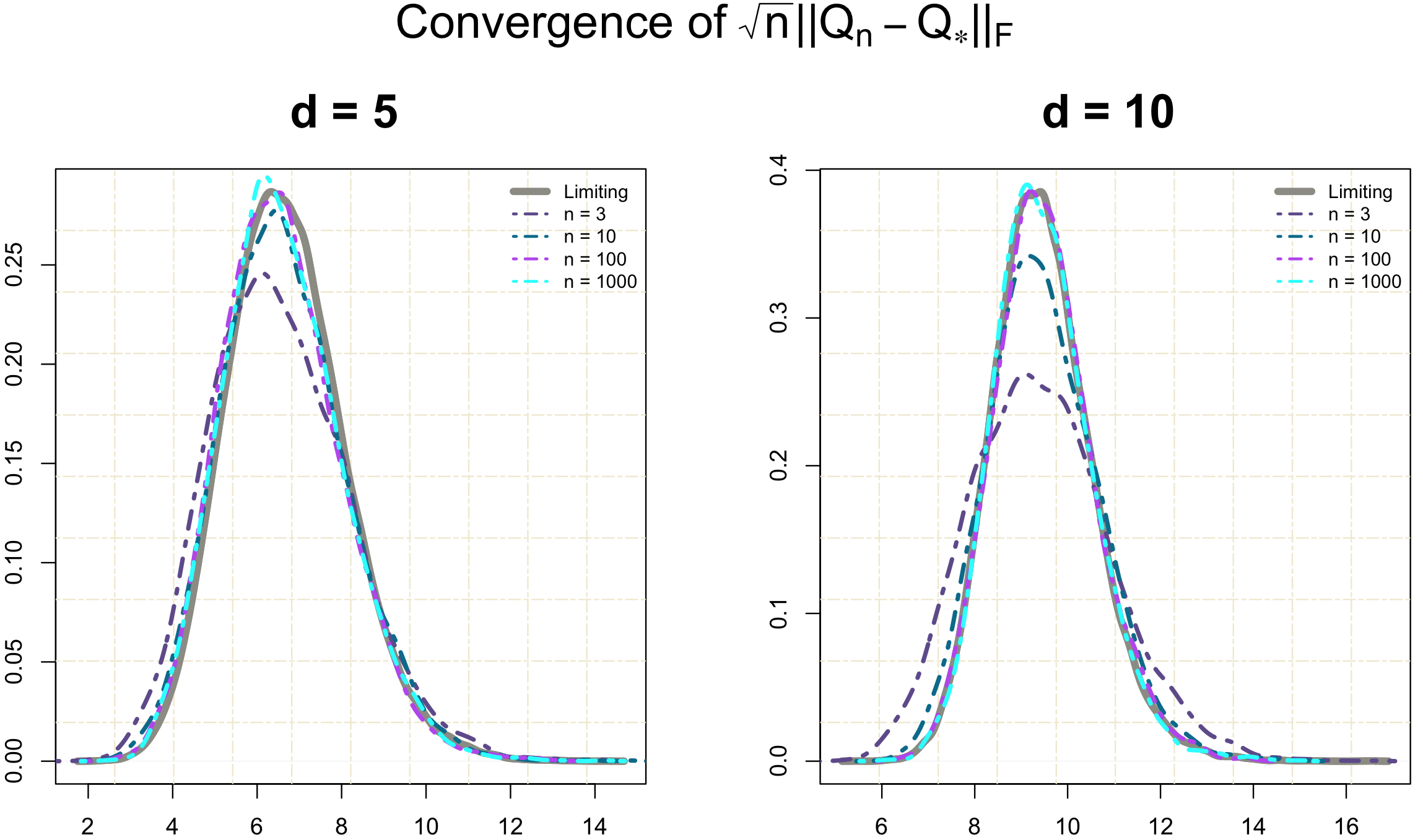
Figure 1: Densities of $\,\mathcal{L}(\sqrt{n}\norm{Q_{n}-Q_{*}}_{F})\,$

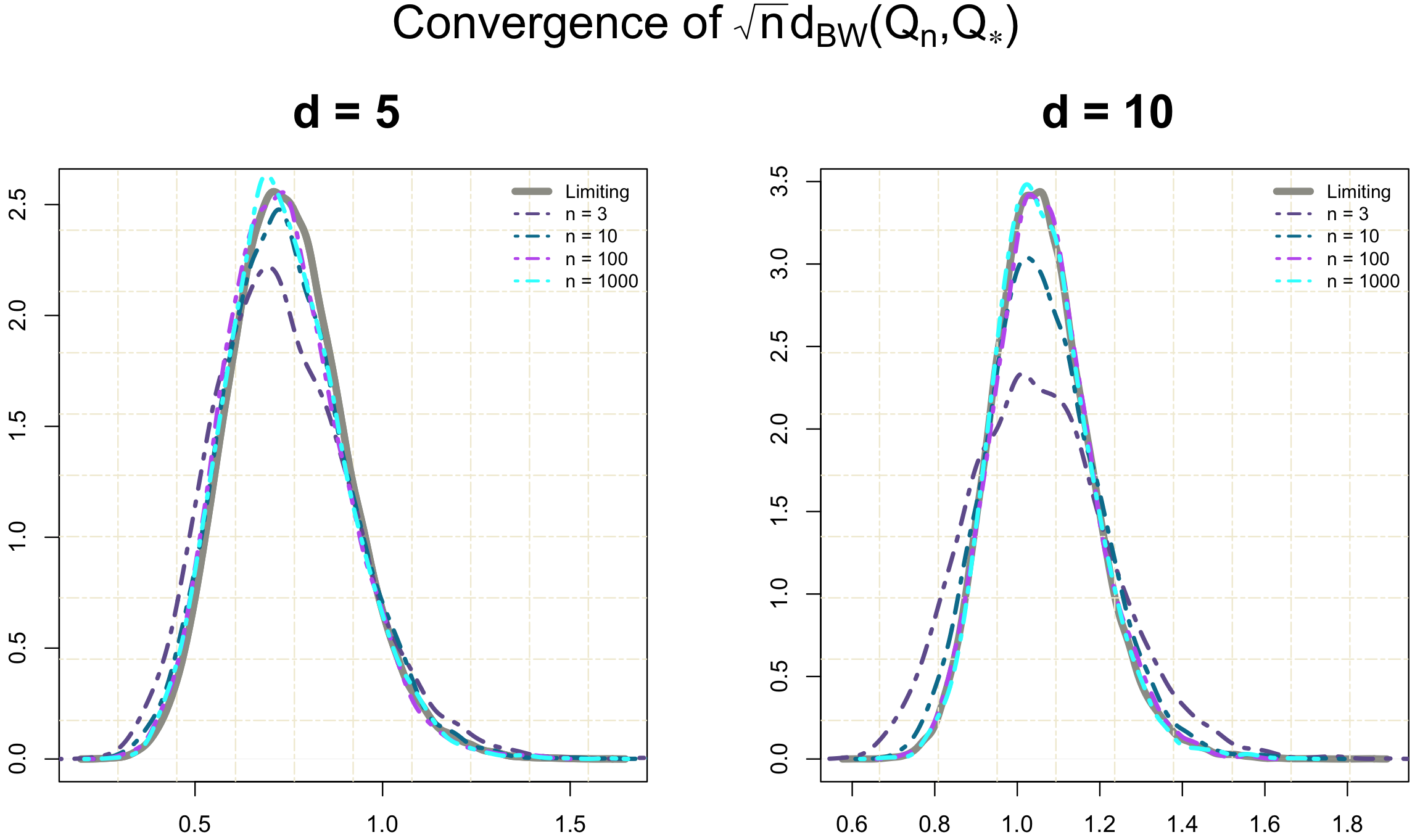
Figure 2: Densities of $\,\mathcal{L}\left(\sqrt{n}d_{BW}(Q_{n},Q_{*})\right)\,$

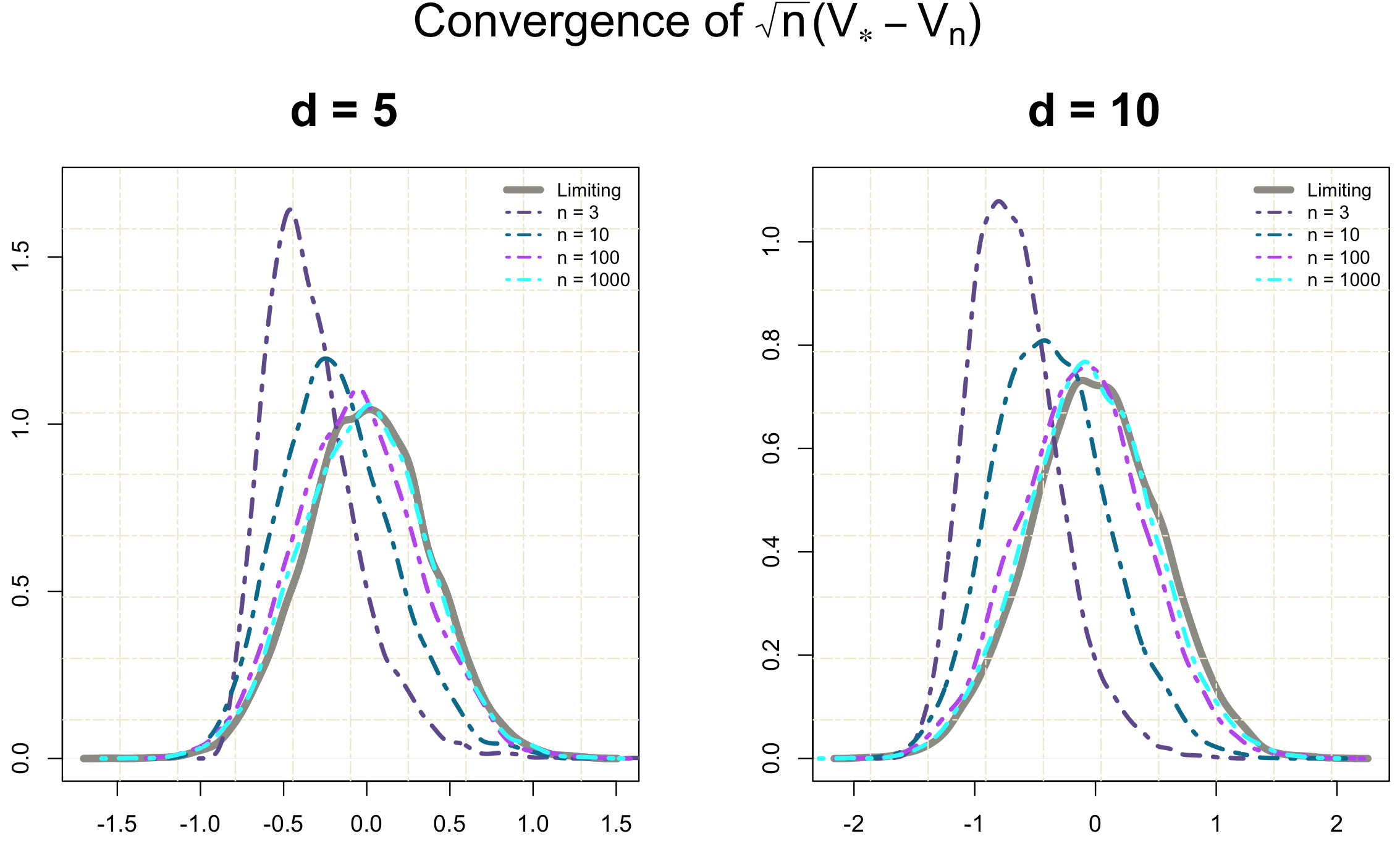
Figure 3: Densities of $\,\mathcal{L}\left(\sqrt{n}(\mathcal{V}_{n}-\mathcal{V}_{*})\right)\,$

4.2 Data aggregation in climate modelling

In this section we carry out the experiments on a family of Gaussian process, using a climate-related data set, collected in Siberia (Russia) between 1930 and 2009 Bulygina and Razuvaev (2012); Tatusko (1990). We set $\,\mathcal{SL}(\mu)\,$ to be a family of Gaussian curves, that describe the daily minimum temperatures within one year, measured at a set of 30 randomly sampled meteorological stations. Each curve is obtained by means of regression and maximum likelihood estimation and is sampled in $\,50\,$ points. More details on this data set are provided in Mallasto and Feragen (2017). The scale-location family under consideration is written as

$$\mathcal{SL}(\mu)=\left\{\nu_{t}=GP(m_{t},S_{t}),~{}m_{t}\in\mathbb{R}^{50},~{}S_{t}\in\mathrm{Sym}_{++}(50),~{}t=1,...,71\right\},$$

where $\,\nu_{t}=GP(m_{t},S_{t})\,$ is a Gaussian process, characterised by mean $\,m_{t}\,$ and covariance $\,S_{t}\,$ inherent to a year $\,t\,$, $\,t\in\{1933,...,2009\}\,$. We let $\,m_{t}=0\,$ for all $\,t\,$. A Gaussian process $\,\mu_{*}=GP(r_{*},Q_{*})\,$ is the population Wasserstein barycenter of $\,\mathcal{SL}(\mu)\,$. It is characterised by $\,(r_{*},Q_{*})\,$

$$r_{*}=0,\quad Q_{*}=\frac{1}{71}\sum^{71}_{t=1}\left(Q^{1/2}_{*}S_{t}Q^{1/2}_{*}\right)^{1/2}.$$

A family of approximating processes$\,\mu_{n}=GP(r_{n},Q_{n})\,$ with parameters $\,(r_{n},Q_{n})\,$ (3.3) is constructed by means of re-sampling with replacement of the original data set. Sample size $\,n\,$ varies in range $\,n=\{3,10,70\}\,$. Fig. 5 and Fig. 5 present densities of $\,\mathcal{L}\left(\sqrt{n}\norm{Q_{n}-Q_{*}}_{F}\right)\,$ and $\,\mathcal{L}\left(\sqrt{n}d_{BW}(Q_{n},Q_{*})\right)\,$ respectively.

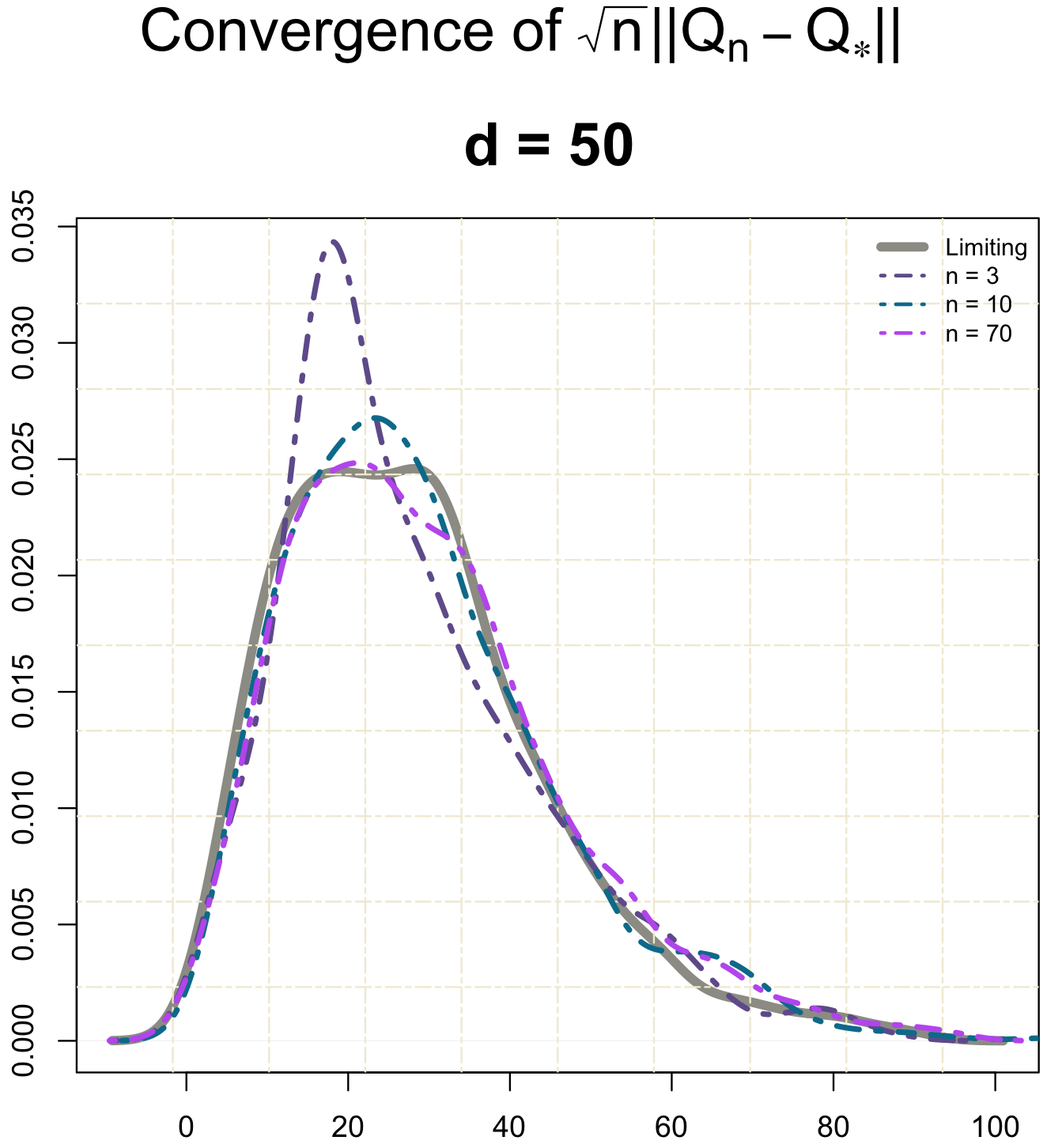
Figure 4: $\,\mathcal{L}\left(\sqrt{n}\norm{Q_{n}-Q_{*}}_{F}\right)\,$

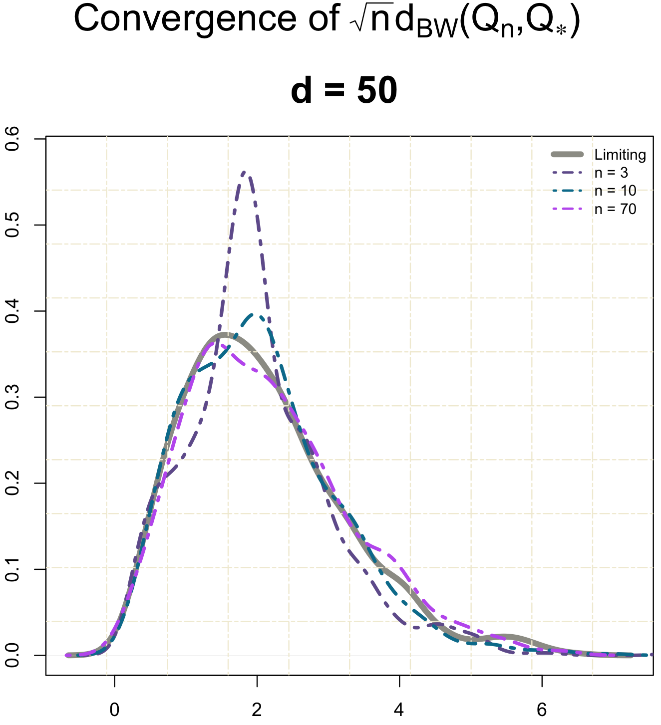
Figure 5: $\,\mathcal{L}\left(\sqrt{n}d_{BW}(Q_{n},Q_{*})\right)\,$

Appendix A Proof of Central Limit Theorem

A.1 Properties of $T_{Q}^{S}$

Proof of Lemma 2.1.

First, we prove that optimal $\,T\,$ is self-adjoint. Indeed, assume the opposite, then

$$Q^{1/2}TQT^{*}Q^{1/2}=\left(Q^{1/2}TQ^{1/2}\right)\left(Q^{1/2}TQ^{1/2}\right)^{*}=Q^{1/2}SQ^{1/2}$$

and thus $\,\operatorname{tr}Q^{1/2}TQ^{1/2}<\operatorname{tr}\left(Q^{1/2}SQ^{1/2}\right)^{1/2}\,$. Therefore

$$\operatorname{tr}(T-I)Q(T^{*}-I) =\operatorname{tr}S+\operatorname{tr}Q-2\operatorname{tr}TQ=\operatorname{tr}S+\operatorname{tr}Q-2\operatorname{tr}Q^{1/2}TQ^{1/2}$$

$$>\operatorname{tr}S+\operatorname{tr}Q-2\operatorname{tr}\left(Q^{1/2}SQ^{1/2}\right)^{1/2}=d_{BW}^{2}(Q,S).$$

If $\,T\,$ is Hermitian but not positive semi-definite, then $\,Q^{1/2}TQ^{1/2}\preccurlyeq\left(Q^{1/2}SQ^{1/2}\right)^{1/2}\,$, $\,Q^{1/2}TQ^{1/2}\neq\left(Q^{1/2}SQ^{1/2}\right)^{1/2}\,$, hence again $\,\operatorname{tr}Q^{1/2}TQ^{1/2}<\operatorname{tr}\left(Q^{1/2}SQ^{1/2}\right)^{1/2}\,$.

Finally, if $\,T\in\mathbb{H}_{+}(n)\,$, then it is straightforward to check that $\,T=T_{Q}^{S}\,$ given by (2.3) and

$$\operatorname{tr}(T-I)Q(T^{*}-I)=\operatorname{tr}S+\operatorname{tr}Q-2\operatorname{tr}\left(Q^{1/2}SQ^{1/2}\right)^{1/2}=d_{BW}^{2}(Q,S).$$

∎

The proof of the Central Limit theorem mainly relies on the differentiability of the map (2.3). Lemma A.2 shows that $\,T_{Q}^{S}\,$ can be linearised in the vicinity of $\,Q\,$:

$$T_{Q+X}^{S}=T_{Q}^{S}+\bm{dT}_{Q}^{S}(X)+o\bigl{(}\norm{X}\bigr{)},$$

where $\,\bm{dT}_{Q}^{S}\colon\mathbb{H}(d)\to\mathbb{H}(d)\,$ is a self-adjoint negative-definite operator and $\,\norm{\cdot}\,$ stands for an operator norm. Properties of $\,\bm{dT}_{Q}^{S}\,$ are investigated in Lemma A.3. Let us introduce some notation: if $\,G(A)\,$ is a functional of a matrix $\,A\,$, then we denote its differential as $\,\bm{d_{A}}G\,$.

Lemma A.1.

Map $\,Q\mapsto g(Q)=Q^{1/2}\,$ is differentiable on $\,\mathbb{H}_{++}(d)\,$, and its differential is given by

$$\bm{d_{Q}}g(X)=U^{*}\left(\frac{(UXU^{*})_{ij}}{\sqrt{q_{i}}+\sqrt{q_{j}}}\right)_{i,j=1}^{d}U,\quad X\in\mathbb{H}(d),$$

where $\,Q=U^{*}\operatorname{diag}(q)U\,$ is the eigenvalue decomposition.

Proof.

First, let us consider the map $\,P\mapsto f(P)=P^{2}\,$. It is smooth and its differential

$$\bm{d_{P}}f(X)=PX+XP,\quad X\in\mathbb{H}(d)$$

is non-degenerated:

$$\langle\bm{d_{P}}f(X),X\rangle=2\operatorname{tr}XPX>0,\quad X\neq 0,$$

whenever $\,P\in\mathbb{H}_{++}(d)\,$. From now on $\,\langle\cdot,\cdot\rangle\,$ denotes a scalar product associated to Frobenius norm.

Now applying the inverse function theorem we obtain that the inverse map $\,g(\cdot)\,$ is also smooth and its differential enjoys the following equation

$$X=\left(\left.\bm{d_{P}}f\right|_{P=Q^{1/2}}\right)\left(\bm{d_{Q}}g(X)\right)=Q^{1/2}\bm{d_{Q}}g(X)+\bm{d_{Q}}g(X)Q^{1/2},$$

thus

$$UXU^{*}=(\operatorname{diag}(q))^{1/2}U\bm{d_{Q}}g(X)U^{*}+U\bm{d_{Q}}g(X)U^{*}(\operatorname{diag}(q))^{1/2},$$

$$(UXU^{*})_{ij}=(\sqrt{q_{i}}+\sqrt{q_{j}})(U\bm{d_{Q}}g(X)U^{*})_{ij},\quad 1\leq i,j\leq d,$$

and

$$\bm{d_{Q}}g(X)=U^{*}\left(\frac{(UXU^{*})_{ij}}{\sqrt{q_{i}}+\sqrt{q_{j}}}\right)_{i,j=1}^{d}U.$$

∎

Lemma A.2 (Fréchet-differentiability of the map $\,T^{S}_{Q}\,$).

For any $\,S\in\mathbb{H}_{+}(d)\,$ the map $\,T_{Q}^{S}\,$ can be linearised in the vicinity of $\,Q\in\mathbb{H}_{++}(d)\,$ as

$$T_{\widetilde{Q}}^{S}=T_{Q}^{S}+\bm{dT}_{Q}^{S}\left(\widetilde{Q}-Q\right)+o\left(\norm{\widetilde{Q}-Q}\right),\quad\text{as}\quad\widetilde{Q}\to Q,$$

where

$$\bm{dT}_{Q}^{S}(X)\stackrel{{\scriptstyle\operatorname{def}}}{{=}}-S^{1/2}U^{*}\varLambda^{-1/2}\delta\varLambda^{-1/2}US^{1/2},\quad X\in\mathbb{H}(d),$$ (A.1)

$\,U^{*}\varLambda U\,$ is an eigenvalue decomposition of $\,S^{1/2}QS^{1/2}\,$

$$U^{*}\varLambda U=S^{1/2}QS^{1/2},\quad U^{*}U=UU^{*}=I,\quad\varLambda=\operatorname{diag}\left(\lambda_{1},\dots,\lambda_{\operatorname{rank}(S)},0,\dots,0\right),$$

$$\varLambda^{-1/2}=\left(\varLambda^{1/2}\right)^{+}=\operatorname{diag}(\lambda_{1}^{-1/2},\dots,\lambda_{\operatorname{rank}(S)}^{-1/2},0,\dots,0),$$

$$\delta=(\delta_{ij})_{i,j=1}^{d},\quad\delta_{ij}=\begin{cases}\frac{\varDelta_{ij}}{\sqrt{\lambda_{i}}+\sqrt{\lambda_{j}}},&i,j\leq\operatorname{rank}(S)\\ 0,&\text{ otherwise}\end{cases},\quad\varDelta=US^{1/2}XS^{1/2}U^{*}.$$

Proof.

The proof mainly relies on the differentiation of the pseudo-inverse term $\,\bigl{(}S^{1/2}QS^{1/2}\bigr{)}^{-1/2}\,$, as soon as

$$\bm{dT}_{Q}^{S}(X)=S^{1/2}\bm{d_{Q}}\left(S^{1/2}QS^{1/2}\right)^{-1/2}(X)S^{1/2}.$$

Obviously we can consider only restriction to $\operatorname{range}(S)$ and therefore assume w.l.o.g. $S\succ 0$. As $\,\left(S^{1/2}(Q+X)S^{1/2}\right)^{-1/2}=U^{*}\left(\varLambda+\varDelta\right)^{-1/2}U\,$, by Lemma A.1 and von Neumann series expansion we obtain for infinitesimal $\,X\in\mathbb{H}(d)\,$ and corresponding $\,\varDelta\,$ that

$$\left(\varLambda+\varDelta\right)^{-1/2} =\left(\varLambda^{1/2}+\delta+o(\norm{\varDelta})\right)^{-1}$$

$$=\Bigl{(}\varLambda^{1/4}\left(I+\varLambda^{-1/4}\delta\varLambda^{-1/4}+o(\norm{\varDelta})\right)\varLambda^{1/4}\Bigr{)}^{-1}$$

$$=\varLambda^{-1/4}\left(I-\varLambda^{-1/4}\delta\varLambda^{-1/4}+o(\norm{\varDelta})\right)\varLambda^{-1/4}$$

$$=\varLambda^{-1/2}-\varLambda^{-1/2}\delta\varLambda^{-1/2}+o(\norm{\varDelta}).$$

Then the differential $\,\bm{d_{Q}}\left(S^{1/2}QS^{1/2}\right)^{-1/2}(X)\,$ is written as

$$\bm{d_{Q}}\left(S^{1/2}QS^{1/2}\right)^{-1/2}(X)=-U^{*}\varLambda^{-1/2}\delta\varLambda^{-1/2}U.$$

Therefore,

$$T^{S}_{Q+X}=T^{S}_{Q}+\bm{dT}_{Q}^{S}(X)+o(\norm{X}),$$

where $\,\bm{dT}_{Q}^{S}(X)\,$ is defined by (A.1). ∎

Lemmas A.3 and A.4 are technical and explore properties of $\,\bm{dT}_{Q}^{S}\,$.

Lemma A.3.

For any $\,S\in\mathbb{H}_{+}(d)\,$, $\,Q\in\mathbb{H}_{++}(d)\,$, the properties of operator $\,\bm{dT}_{Q}^{S}\,$ defined in (A.1) are following:

1. it is self-adjoint;

2. it is negative semi-definite;

3. it enjoys the following bounds:

   $$-\left\langle\bm{dT}_{Q}^{S}(X),X\right\rangle \leq\frac{\lambda_{max}^{1/2}\left(S^{1/2}QS^{1/2}\right)}{2}\norm{Q^{-1/2}XQ^{-1/2}}_{F}^{2},$$

   $$-\left\langle\bm{dT}_{Q}^{S}(X),X\right\rangle \geq\frac{\lambda_{min}^{1/2}\left(S^{1/2}QS^{1/2}\right)}{2}\norm{Q^{-1/2}XQ^{-1/2}}_{F}^{2};$$

4. it is homogeneous w.r.t. $Q$ with degree $-\frac{3}{2}$ and w.r.t. $S$ with degree $\frac{1}{2}$, i.e. $\,\bm{dT}_{aQ}^{S}=a^{-3/2}\bm{dT}_{Q}^{S}\,$ and $\,\bm{dT}_{Q}^{aS}=a^{1/2}\bm{dT}_{Q}^{S}\,$ for any $a>0$;

5. it is monotone w.r.t. $S^{1/2}QS^{1/2}$ (once range $S$ is fixed): $\,\bm{dT}_{Q_{0}}^{S_{0}}\preccurlyeq\bm{dT}_{Q_{1}}^{S_{1}}\,$ in the sense of self-adjoint operators on $\mathbb{H}(d)$ whenever $\,S_{0}^{1/2}Q_{0}S_{0}^{1/2}\preccurlyeq S_{1}^{1/2}Q_{1}S_{1}^{1/2}\,$ and $\,\operatorname{range}(S_{0})=\operatorname{range}(S_{1})\,$; in particular, $\bm{dT}_{Q}^{S}$ is monotone w.r.t. $Q\in\mathbb{H}_{++}(d)$ for fixed $S$.

Proof.

Slightly changing notations, we rewrite (A.1) as

$$\bm{dT}_{Q}^{S}(X)=-S^{1/2}U^{*}\varLambda^{-1/2}\delta^{X}\varLambda^{-1/2}US^{1/2},$$

where matrices $\,U,U^{*}\,$ and $\,\varLambda\,$ come from Lemma A.2 and

$$\delta^{X}=(\delta^{X}_{ij})_{i,j=1}^{d},\quad\delta^{X}_{ij}=\frac{\varDelta^{X}_{ij}}{\sqrt{\lambda_{i}}+\sqrt{\lambda_{j}}},\quad\varDelta^{X}=US^{1/2}XS^{1/2}U^{*}.$$

(I) Self-adjointness

Consider a scalar product

$$\langle\bm{dT}_{Q}^{S}(X),Y\rangle=\operatorname{tr}\bigl{(}\bm{dT}_{Q}^{S}(X)Y\bigr{)} =-\operatorname{tr}\bigl{(}S^{1/2}U^{*}\varLambda^{-1/2}\delta^{X}\varLambda^{-1/2}US^{1/2}Y\bigr{)}$$

$$=-\operatorname{tr}\bigl{(}\varLambda^{-1/2}\delta^{X}\varLambda^{-1/2}US^{1/2}YS^{1/2}U^{*}\bigr{)}.$$

We now introduce a following notation

$$\varDelta^{Y}\stackrel{{\scriptstyle\operatorname{def}}}{{=}}US^{1/2}YS^{1/2}U^{*}.$$

Then the above equality can be continued as follows:

$$- \operatorname{tr}\bigl{(}\varLambda^{-1/2}\delta^{X}\varLambda^{-1/2}US^{1/2}YS^{1/2}U^{*}\bigr{)}=-\operatorname{tr}\bigl{(}\varLambda^{-1/2}\delta^{X}\varLambda^{-1/2}\varDelta^{Y}\bigr{)}$$

$$\qquad=-\sum_{i,j=1}^{r}\frac{\delta^{X}_{ij}}{\sqrt{\lambda_{i}\lambda_{j}}}\varDelta^{Y}_{ij}=-\sum_{i,j=1}^{r}\frac{\varDelta^{X}_{ij}\varDelta^{Y}_{ij}}{\sqrt{\lambda_{i}\lambda_{j}}(\sqrt{\lambda_{i}}+\sqrt{\lambda_{j}})}$$

$$\qquad=\operatorname{tr}\bigl{(}\bm{dT}_{Q}^{S}(Y)X\bigr{)}=\operatorname{tr}\bigl{(}X\bm{dT}_{Q}^{S}(Y)\bigr{)}=\langle X,\bm{dT}_{Q}^{S}(Y)\rangle,$$

where $\,r=\operatorname{rank}(S)\,$. Thus the operator is self-adjoint.

(II) Boundedness and (III) eigenvalues

Denoting $\,\varDelta^{X}\,$ by $\,\varDelta\,$ (i.e. now $\,\varDelta=US^{1/2}XS^{1/2}U^{*}\,$) and taking into account the above expansion of an inner product, one obtains

$$-\langle\bm{dT}_{Q}^{S}(X),X\rangle=\sum_{i,j=1}^{r}\frac{\varDelta^{2}_{ij}}{\sqrt{\lambda_{i}\lambda_{j}}(\sqrt{\lambda_{i}}+\sqrt{\lambda_{j}})}=\sum_{i,j=1}^{r}\left(\frac{\varDelta_{ij}}{\sqrt{\lambda_{i}\lambda_{j}}}\right)^{2}\frac{\sqrt{\lambda_{i}\lambda_{j}}}{\sqrt{\lambda_{i}}+\sqrt{\lambda_{j}}}.$$ (A.2)

Note, that the function $\,f(\lambda_{i},\lambda_{j})\stackrel{{\scriptstyle\operatorname{def}}}{{=}}\frac{\sqrt{\lambda_{i}\lambda_{j}}}{\sqrt{\lambda_{i}}+\sqrt{\lambda_{j}}}\,$ is monotonously increasing in both arguments $\,\lambda_{i}\,$ and $\,\lambda_{j}\,$, thus

$$\max_{i,j}f(\lambda_{i},\lambda_{j})=\frac{\lambda_{max}^{1/2}(\varLambda)}{2},\quad\min_{i,j}f(\lambda_{i},\lambda_{j})=\frac{\lambda_{min}^{1/2}(\varLambda)}{2}.$$ (A.3)

For the sake of simplicity we introduce a new variable

$$\zeta\stackrel{{\scriptstyle\operatorname{def}}}{{=}}Q^{-1/2}XQ^{-1/2},$$

its Frobenius norm is written as

$$\norm{\zeta}_{F}^{2}=\operatorname{tr}\bigl{(}XQ^{-1}XQ^{-1}\bigr{)}.$$

Moreover, the following inequality for trace holds:

$$\operatorname{tr}\bigl{(}XQ^{-1}XQ^{-1}\bigr{)} \geq\operatorname{tr}\bigl{(}\varPi_{S}X\varPi_{S}Q^{-1}\varPi_{S}X\varPi_{S}Q^{-1}\varPi_{S}\bigr{)}$$

$$=\operatorname{tr}\bigl{(}\varDelta\varLambda^{+}\varDelta\varLambda^{+}\bigr{)}=\norm{\varLambda^{-1/2}\varDelta\varLambda^{-1/2}}_{F}^{2}=\sum_{i,j=1}^{r}\frac{\varDelta_{ij}^{2}}{\lambda_{i}\lambda_{j}}.$$

Here $\,\varPi_{S}\,$ is the orthogonal projector onto range of $\,S\,$.

Then combining (A.2) with (A.3), the upper and lower bounds can be obtained as follows:

$$-\langle\bm{dT}_{Q}^{S}(X),X\rangle \leq\max_{i,j}f(\lambda_{i},\lambda_{j})\sum_{i,j=1}^{r}\left(\frac{\varDelta_{ij}}{\sqrt{\lambda_{i}\lambda_{j}}}\right)^{2}\leq\frac{\lambda_{max}^{1/2}(\varLambda)}{2}\norm{\zeta}_{F}^{2},$$

$$-\langle\bm{dT}_{Q}^{S}(X),X\rangle \geq\min_{i,j}f(\lambda_{i},\lambda_{j})\sum_{i,j=1}^{r}\left(\frac{\varDelta_{ij}}{\sqrt{\lambda_{i}\lambda_{j}}}\right)^{2}=\frac{\lambda_{min}^{1/2}(\varLambda)}{2}\norm{\zeta}_{F}^{2}.$$

Note, that if $\,S\,$ is degenerated, the lower bound becomes trivial.

(IV) Homogeneity and (V) monotonicity

Homogeneity follows directly from definition (A.1). Now we prove monotonicity. As range of $\,S^{1/2}QS^{1/2}\,$ is fixed, we may assume $\,S\succ 0\,$. Consider

$$\langle\bm{dT}_{Q}^{S}(X),X\rangle =\operatorname{tr}\left(S^{1/2}U^{*}\varLambda^{-1/2}\delta\varLambda^{-1/2}US^{1/2},X\right)$$

$$=\left\langle U^{*}\varLambda^{-1/2}\delta\varLambda^{-1/2}U,S^{1/2}XS^{1/2}\right\rangle$$

$$=\left\langle\bm{d_{Q}}\left(S^{1/2}QS^{1/2}\right)^{-1/2}(X),S^{1/2}XS^{1/2}\right\rangle$$

$$=\left\langle\bm{d_{M}}M^{-1/2}\left(S^{1/2}XS^{1/2}\right),S^{1/2}XS^{1/2}\right\rangle,$$

with replacement $\,M=S^{1/2}QS^{1/2}\,$ to be change of variables. As soon as $\,X\,$ is supposed to be fixed, it is enough to show that the differential $\,\bm{d_{M}}M^{-1/2}\,$ is monotone in $\,M\,$. Notice that the operator $\,\left(\bm{d_{M}}M^{-1/2}\right)^{-1}\,$ at point $M$ is equal to the differential of the inverse map $\,P\mapsto P^{-2}\,$ at point $\,P=M^{-1/2}\,$:

$$\bm{d_{M}}M^{-1/2}=\left(\left.\bm{d_{P}}P^{-2}\right|_{P=M^{-1/2}}\right)^{-1}.$$

In turn, $\,\bm{d_{P}}P^{-2}\,$ can be expressed as

$$\bm{d_{P}}P^{-2}(X)=-P^{-1}\left(P^{-1}X+XP^{-1}\right)P^{-1},$$

the right part of the above equation is self-adjoint, negative-definite and

$$\left\langle-P^{-1}\left(P^{-1}X+XP^{-1}\right)P^{-1},X\right\rangle=-2\operatorname{tr}P^{-2}XP^{-1}X.$$

Choose $\,M_{1}\succcurlyeq M_{0}\succ 0\,$ (thus $\,M_{1}^{1/2}\succcurlyeq M_{0}^{1/2}\,$) and let $\,P_{i}=M_{i}^{-1/2}\,$ for $\,i=0,1\,$. Then for any fixed $\,X\in\mathbb{H}(d)\,$

$$-\operatorname{tr}P_{1}^{-2}XP_{1}^{-1}X=-\operatorname{tr}M_{1}XM_{1}^{1/2}X\leq-\operatorname{tr}M_{0}XM_{0}^{1/2}X=-\operatorname{tr}P_{0}^{-2}XP_{0}^{-1}X,$$

i.e. $\,\left.\bm{d_{P}}P^{-2}\right|_{P_{1}}\preccurlyeq\left.\bm{d_{P}}P^{-2}\right|_{P_{0}}\,$ and hence for the differential of $\,M\mapsto M^{-1/2}\,$ the inverse inequality holds: $\,\left.\bm{d_{M}}M^{-1/2}\right|_{M_{0}}\preccurlyeq\left.\bm{d_{M}}M^{-1/2}\right|_{M_{1}}\,$. This entails monotonicity of $\,\bm{dT}_{Q}^{S}\,$. ∎

Corollary A.1.

We define a following rescaled operator

$$\bm{dt}_{Q}^{S}(\zeta)\stackrel{{\scriptstyle\operatorname{def}}}{{=}}Q^{1/2}\bm{dT}_{Q}^{S}\left(Q^{1/2}\zeta Q^{1/2}\right)Q^{1/2},\quad\zeta\in\mathbb{H}(d).$$ (A.4)

Then a following bound on its eigenvalues hold:

$$\lambda_{min}\left(-\bm{dt}_{Q}^{S}\right)=\frac{1}{2}\lambda_{min}^{1/2}\left(S^{1/2}QS^{1/2}\right),$$

$$\lambda_{max}\left(-\bm{dt}_{Q}^{S}\right)=\frac{1}{2}\lambda_{max}^{1/2}\left(S^{1/2}QS^{1/2}\right).$$

Proof.

Notice that inequalities

$$\lambda_{min}\left(-\bm{dt}_{Q}^{S}\right)\geq\frac{1}{2}\lambda_{min}^{1/2}\left(S^{1/2}QS^{1/2}\right),$$

$$\lambda_{max}\left(-\bm{dt}_{Q}^{S}\right)\leq\frac{1}{2}\lambda_{max}^{1/2}\left(S^{1/2}QS^{1/2}\right),$$

are a trivial consequence of Lemma A.3 (III). Now defining for any $\,1\leq k\leq\operatorname{rank}(S)\,$

$$\varDelta_{ij}^{k}=\begin{cases}1,&i=j=k,\\ 0,&\text{otherwise},\end{cases},\quad X^{k}=S^{-1/2}U\varDelta^{k}U^{*}S^{-1/2},\quad\zeta^{k}=Q^{-1/2}X^{k}Q^{-1/2}$$

we obtain from (A.2) that

$$-\left\langle\bm{dt}_{Q}^{S}(\zeta^{k}),\zeta^{k}\right\rangle=-\left\langle\bm{dT}_{Q}^{S}(X^{k}),X^{k}\right\rangle=\frac{\lambda_{k}^{1/2}}{2}\norm{\zeta^{k}}_{F}^{2}.$$

Therefore, the above inequalities are sharp. ∎

Lemma A.4.

For any $\,Q_{0},Q_{1}\in\mathbb{H}_{++}(d)\,$, $\,S\in\mathbb{H}_{+}(d)\,$ consider

$$Q_{t}\stackrel{{\scriptstyle\operatorname{def}}}{{=}}(1-t)Q_{0}+tQ_{1},\quad Q^{\prime}\stackrel{{\scriptstyle\operatorname{def}}}{{=}}Q_{0}^{-1/2}Q_{1}Q_{0}^{-1/2}.$$ (A.5)

Then

$$\frac{2}{\lambda_{min}(Q^{\prime})+{\lambda_{min}^{1/2}(Q^{\prime})}}\bm{dT}_{Q_{0}}^{S} \preccurlyeq\int_{0}^{1}\bm{dT}_{Q_{t}}^{S}\,dt$$ (I)

$$\preccurlyeq\frac{2}{\lambda_{max}(Q^{\prime})+{\lambda_{max}^{1/2}(Q^{\prime})}}\bm{dT}_{Q_{0}}^{S}$$

$$\preccurlyeq\frac{1}{1+3\norm{Q^{\prime}-I}/4}\bm{dT}_{Q_{0}}^{S}.$$

Moreover, if $\,\norm{Q^{\prime}-I}<1\,$, then

$$\int_{0}^{1}\bm{dT}_{Q_{t}}^{S}\,dt\succcurlyeq\frac{1}{1-\norm{Q^{\prime}-I}}\bm{dT}_{Q_{0}}^{S}.$$ (II)

Remark 2.

The above inequality might seem confusing due to the fact that $\,\lambda_{min}(\cdot)\leq\lambda_{max}(\cdot)\,$, however this is explained by the fact that $\,\bm{dT}_{Q}^{S}\,$ is negative definite.

Proof.

Notice that

$$Q_{t}=Q_{0}^{1/2}\bigl{(}(1-t)I+tQ^{\prime}\bigr{)}Q_{0}^{1/2}.$$

Monotonicity and homogeneity with degree $\,-\frac{3}{2}\,$ of $\,\bm{dT}_{Q}^{S}(\cdot)\,$ (see Lemma A.3) yield

$$\bm{dT}_{Q_{t}}^{S} \preccurlyeq\bm{dT}_{((1-t)+t\lambda_{max}(Q^{\prime}))Q_{0}}^{S}$$

$$=\bigl{(}(1-t)+t\lambda_{max}(Q^{\prime})\bigr{)}^{-3/2}\bm{dT}_{Q_{0}}^{S}$$

and

$$\bm{dT}_{Q_{t}}^{S} \succcurlyeq\bm{dT}_{((1-t)+t\lambda_{min}(Q^{\prime}))Q_{0}}^{S}$$

$$=\bigl{(}(1-t)+t\lambda_{min}(Q^{\prime})\bigr{)}^{-3/2}\bm{dT}_{Q_{0}}^{S}.$$

Therefore,

$$\int_{0}^{1}\bm{dT}_{Q_{t}}^{S}\,dt \preccurlyeq\bm{dT}_{Q_{0}}^{S}\int_{0}^{1}\bigl{(}(1-t)+t\lambda_{max}(Q^{\prime})\bigr{)}^{-3/2}\,dt$$

$$=\frac{2}{\lambda_{max}(Q^{\prime})+{\lambda_{max}^{1/2}(Q^{\prime})}}\bm{dT}_{Q_{0}}^{S}$$

and respectively,

$$\int_{0}^{1}\bm{dT}_{Q_{t}}^{S}\,dt\succcurlyeq\frac{2}{\lambda_{min}(Q^{\prime})+{\lambda_{min}^{1/2}(Q^{\prime})}}\bm{dT}_{Q_{0}}^{S}.$$

The rest of the Lemma follow from the fact that

$$\lambda_{min}(Q^{\prime})\geq 1-\norm{Q^{\prime}-I},\quad\lambda_{max}(Q^{\prime})\leq 1+\norm{Q^{\prime}-I}$$

and inequalities

$$\sqrt{1+x}\leq 1+\frac{x}{2}\text{~{}~{}for~{}~{}}x\geq 0,$$

$$\sqrt{1-x}\geq 1-x\text{~{}~{}for~{}~{}}0\leq x\leq 1.$$

∎

A.2 Properties of $\,d_{BW}(Q,S)\,$

The next lemma ensures strict convexity of $\,d_{BW}(Q,S)\,$. In essence, the proof mainly relies on Theorem 7 Bhatia et al. (2018).

Lemma A.5.

For any $\,S\in\mathbb{H}_{+}(d)\,$ function $\,Q\mapsto d_{BW}^{2}(Q,S)\,$ is convex on $\,\mathbb{H}_{+}(d)\,$. Moreover, if $\,S\succ 0\,$, then it is strictly convex.

Proof.

According to (Bhatia et al., 2018, Theorem 7) function $\,h(X)=\operatorname{tr}X^{1/2}\,$ is strictly concave on $\,\mathbb{H}_{+}(d)\,$, hence function

$$Q\mapsto d_{BW}^{2}(Q,S)=\operatorname{tr}S+\operatorname{tr}Q-2\operatorname{tr}\left(S^{1/2}QS^{1/2}\right)^{1/2}$$

is convex on $\,\mathbb{H}_{+}(d)\,$ for any positive semi-definite $\,S\,$. Moreover, if $\,S\succ 0\,$, then $\,Q\mapsto S^{1/2}QS^{1/2}\,$ is an injective linear map, and therefore $\,d_{BW}^{2}(Q,S)\,$ is strictly convex. ∎

Further we present differentiability of $\,d_{BW}(Q,S)\,$ and its quadratic approximation.

Lemma A.6.

For any $\,Q\in\mathbb{H}_{++}(d)\,$, $\,S\in\mathbb{H}_{+}(d)\,$ function $\,d_{BW}^{2}(Q,S)\,$ is twice differentiable in $Q$ with

$$\bm{d_{Q}}d_{BW}^{2}(Q,S)(X)=\langle I-T_{Q}^{S},X\rangle, X\in\mathbb{H}(d),$$

$$\bm{d^{2}_{Q}}d_{BW}^{2}(Q,S)(X,Y)=-\langle X,\bm{dT}_{Q}^{S}(Y)\rangle, X,Y\in\mathbb{H}(d).$$

Moreover, the following quadratic approximation holds: for any $\,Q_{0},Q_{1}\in\mathbb{H}_{++}(d)\,$

$$-\tfrac{2}{\left(1+\lambda_{max}^{1/2}(Q^{\prime})\right)^{2}} \left\langle\bm{dT}_{Q_{0}}^{S}(Q_{1}-Q_{0}),Q_{1}-Q_{0}\right\rangle$$

$$\leq d_{BW}^{2}(Q_{1},S)-d_{BW}^{2}(Q_{0},S)+\langle T_{Q_{0}}^{S}-I,Q_{1}-Q_{0}\rangle$$

$$\leq-\tfrac{2}{\left(1+\lambda_{min}^{1/2}(Q^{\prime})\right)^{2}}\left\langle\bm{dT}_{Q_{0}}^{S}(Q_{1}-Q_{0}),Q_{1}-Q_{0}\right\rangle.$$

with $\,Q^{\prime}\,$ defined in (A.5).

Proof.

Note that

$$\bm{d_{Q}}\left(S^{1/2}QS^{1/2}\right)^{1/2}(X)=U^{*}\delta U,$$

where $\,\delta\,$ comes from Lemma A.2. Furthermore, Lemma A.1 implies that

$$\bm{d_{Q}}\operatorname{tr}\left(S^{1/2}QS^{1/2}\right)^{1/2}(X) =\operatorname{tr}\bm{d_{Q}}\left(S^{1/2}QS^{1/2}\right)^{1/2}(X)=\operatorname{tr}\delta$$

$$=\sum_{i=1}^{\operatorname{rank}(S)}\frac{\varDelta_{ii}}{2\sqrt{\lambda_{i}}}=\frac{1}{2}\operatorname{tr}\varDelta\varLambda^{-1/2}$$

$$=\frac{1}{2}\operatorname{tr}S^{1/2}XS^{1/2}\left(S^{1/2}QS^{1/2}\right)^{-1/2}=\frac{1}{2}\left\langle T_{Q}^{S},X\right\rangle.$$

Consequently, $\,d_{BW}^{2}(Q,S)\,$ is differentiable and

$$\bm{d_{Q}}d_{BW}^{2}(Q,S)(X)=\operatorname{tr}X-2\bm{d_{Q}}\operatorname{tr}\left(S^{1/2}QS^{1/2}\right)^{1/2}(X)=\left\langle I-T_{Q}^{S},X\right\rangle.$$

Applying Lemma A.2 one obtains

$$\bm{d^{2}_{Q}}d_{BW}^{2}(Q,S)(X,Y)=\bm{d_{Q}}\left\langle I-T_{Q}^{S},X\right\rangle=-\left\langle\bm{dT}_{Q}^{S}(Y),X\right\rangle(Y).$$

Quadratic approximation

Let $\,Q_{0},Q_{1}\in\mathbb{H}_{++}(d)\,$, $\,Q_{t}\stackrel{{\scriptstyle\operatorname{def}}}{{=}}(1-t)Q_{0}+tQ_{1}\,$, $\,t\in[0,1]\,$. The Taylor expansion in integral form applied to $\,d_{BW}^{2}(Q_{t},S)\,$ implies

$$d_{BW}^{2}(Q_{1},S) =d_{BW}^{2}(Q_{0},S)+\left\langle I-T_{Q_{0}}^{S},Q_{1}-Q_{0}\right\rangle$$

$$\quad\quad+\int_{0}^{1}(1-t)\left\langle-\bm{dT}_{Q_{t}}^{S}(Q_{1}-Q_{0}),Q_{1}-Q_{0}\right\rangle\,dt$$

$$=d_{BW}^{2}(Q_{0},S)-\left\langle T_{Q_{0}}^{S}-I,Q_{1}-Q_{0}\right\rangle$$

$$\quad\quad-\left\langle\left[\int_{0}^{1}(1-t)\bm{dT}_{Q_{t}}^{S}\,dt\right](Q_{1}-Q_{0}),Q_{1}-Q_{0}\right\rangle.$$

Following the same ideas as in the proof of Lemma A.4 one obtains that

$$\int_{0}^{1}(1-t)\bm{dT}_{Q_{t}}^{S}\,dt \preccurlyeq\int_{0}^{1}(1-t)\bigl{(}(1-t)+t\lambda_{max}(Q^{\prime})\bigr{)}^{-3/2}\bm{dT}_{Q_{0}}^{S}\,dt$$

$$=\tfrac{2}{\left(1+\lambda_{max}^{1/2}(Q^{\prime})\right)^{2}}\bm{dT}_{Q_{0}}^{S}$$

and

$$\int_{0}^{1}(1-t)\bm{dT}_{Q_{t}}^{S}\,dt\succcurlyeq\tfrac{2}{\left(1+\lambda_{min}^{1/2}(Q^{\prime})\right)^{2}}\bm{dT}_{Q_{0}}^{S}.$$

Thus

$$-\tfrac{2}{\left(1+\lambda_{max}^{1/2}(Q^{\prime})\right)^{2}} \left\langle\bm{dT}_{Q_{0}}^{S}(Q_{1}-Q_{0}),Q_{1}-Q_{0}\right\rangle$$

$$\leq d_{BW}^{2}(Q_{1},S)-d_{BW}^{2}(Q_{0},S)+\langle T_{Q_{0}}^{S}-I,Q_{1}-Q_{0}\rangle$$

$$\leq-\tfrac{2}{\left(1+\lambda_{min}^{1/2}(Q^{\prime})\right)^{2}}\left\langle\bm{dT}_{Q_{0}}^{S}(Q_{1}-Q_{0}),Q_{1}-Q_{0}\right\rangle.$$

∎

A.3 Central limit theorem for $\,Q_{n}\,$

First let us prove uniqueness and positive-definiteness of Bures–Wasserstein barycenter.

Proof of Theorem 2.1.

Since

$$\mathbb{E}d_{BW}^{2}(0,S)=\mathbb{E}\operatorname{tr}S<\infty$$

and $\,d_{BW}(Q,S)\to\infty\,$ as $\,\norm{Q}\to\infty\,$, the barycenter $\,Q_{*}\,$ always exists by continuity and compactness argument. In case $\,\mathbb{P}(\mathbb{H}_{++}(d))>0\,$ applying Lemma A.5 we obtain strict convexity of the integral

$$Q\mapsto\mathbb{E}d_{BW}^{2}(Q,S)=\mathcal{V}(Q),\quad Q\in\mathbb{H}_{+}(d),$$

and therefore, uniqueness of the minimizer $\,Q_{*}\,$.

To prove that $\,Q_{*}\succ 0\,$ consider arbitrary degenerated $\,Q_{0}\in\mathbb{H}_{+}(d)\cap\mathbb{A}\,$, $\,Q_{1}\in\mathbb{H}_{++}(d)\cap\mathbb{A}\,$ (which exists by Assumption 3) and $\,S\in\mathbb{H}_{++}(d)\,$. Let us define $\,Q_{t}=(1-t)Q_{0}+tQ_{1}\in\mathbb{A}\,$. We are going to show, that

$$\frac{d}{dt}d_{BW}^{2}(Q_{t},S)=\langle I-T_{Q_{t}}^{S},Q_{1}-Q_{0}\rangle\to-\infty\quad\text{as}\quad t\to 0.$$

Consider eigen-decomposition $\,S^{1/2}Q_{0}S^{1/2}=U^{*}\varLambda U\,$, $\,\varLambda=\operatorname{diag}(\lambda_{1},\dots,\lambda_{r},0,\dots,0)\,$, where $\,r=\operatorname{rank}(Q_{0})\,$. Respectively, we write $\,C=US^{1/2}Q_{1}S^{1/2}U^{*}\,$ in a block form

$$C=\begin{pmatrix}C_{11}&C_{12}\\ C_{21}&C_{22}\end{pmatrix},\quad C_{11}\in\mathbb{H}_{++}(r),\;C_{12}=C_{21}^{*}\in\mathbb{C}^{r\times(d-r)},\;C_{22}\in\mathbb{H}_{++}(d-r).$$

Cramer’s rule for inverse matrix and Laplace’s formula yield

$$U\left(S^{1/2}Q_{t}S^{1/2}\right)^{-1}U^{*}=\bigl{(}(1-t)\varLambda+tC\bigr{)}^{-1}=\begin{pmatrix}O(1)&O(1)\\ O(1)&C_{22}^{-1}/t+O(1)\end{pmatrix},\text{ as }t\to 0,$$

therefore

$$\sqrt{t}U\left(S^{1/2}Q_{t}S^{1/2}\right)^{-1/2}U^{*}\to\begin{pmatrix}0&0\\ 0&C_{22}^{-1/2}\end{pmatrix}.$$

Consequently,

$$\sqrt{t}\left\langle T_{Q_{t}}^{S},Q_{0}\right\rangle =\sqrt{t}\left\langle\left(S^{1/2}Q_{t}S^{1/2}\right)^{-1/2},S^{1/2}Q_{0}S^{1/2}\right\rangle$$

$$=\left\langle\sqrt{t}U\left(S^{1/2}Q_{t}S^{1/2}\right)^{-1/2}U^{*},US^{1/2}Q_{0}S^{1/2}U^{*}\right\rangle$$

$$=\left\langle\begin{pmatrix}o(1)&o(1)\\ o(1)&C_{22}^{-1/2}\end{pmatrix},\begin{pmatrix}\operatorname{diag}(\lambda_{1},\dots,\lambda_{r})&0\\ 0&0\end{pmatrix}\right\rangle=o(1).$$

In the same way one can obtain

$$\sqrt{t}\left\langle T_{Q_{t}}^{S},Q_{1}\right\rangle=\left\langle\begin{pmatrix}o(1)&o(1)\\ o(1)&C_{22}^{-1/2}\end{pmatrix},\begin{pmatrix}C_{11}&C_{12}\\ C_{21}&C_{22}\end{pmatrix}\right\rangle=\operatorname{tr}C_{22}^{1/2}+o(1).$$

Consequently,

$$\frac{d}{dt}d_{BW}^{2}(Q_{t},S)=\langle I-T_{Q_{t}}^{S},Q_{1}-Q_{0}\rangle=\operatorname{tr}Q_{1}-\operatorname{tr}Q_{0}-\frac{\operatorname{tr}C_{22}^{1/2}+o(1)}{\sqrt{t}}\to-\infty.$$

Since $\,\mathbb{P}(\mathbb{H}_{++}(d))>0\,$ by Assumption 3 and $\,d_{BW}^{2}(Q,S)\,$ is convex, we conclude that

$$\frac{d}{dt}\mathcal{V}(Q_{t})=\mathbb{E}\frac{d}{dt}d_{BW}^{2}(Q_{t},S)\to-\infty\quad\text{as}\quad t\to 0,$$

thus $\,Q_{0}\,$ cannot be a barycenter of $\mathbb{P}$. This yields $\,Q_{*}\succ 0\,$.

Since $\mathcal{V}(\cdot)$ is convex and barycenter of $\mathbb{P}$ is positive-definite and unique, it is characterized as a stationary point of Fréchet variation on subspace $\mathbb{A}$, i.e. as a solution to equation

$$\bm{\varPi}_{\mathbb{M}}\nabla\mathcal{V}(Q)=\bm{\varPi}_{\mathbb{M}}(I-\mathbb{E}T_{Q}^{S})=0,\quad Q\in\mathbb{A}\cap\mathbb{H}_{++}(d),$$

as required. ∎

The proof of CLT widely uses the concept of covariance operators on the space of optimal transportation maps and on the space of covariance matrices.

Covariance operator on the space of optimal maps

Consider $\,T_{i}\stackrel{{\scriptstyle\operatorname{def}}}{{=}}T_{Q_{*}}^{S_{i}}\,$ and $\,T^{n}_{i}\stackrel{{\scriptstyle\operatorname{def}}}{{=}}T_{Q_{n}}^{S_{i}}\,$. We define covariance $\,\bm{\varSigma}\,$ of $\,T_{i}\,$, its empirical counterpart $\,\bm{\varSigma_{n}}\,$, and its data-driven estimator $\,\bm{\hat{\varSigma}_{n}}\,$ as follows

$$\bm{\varSigma}\stackrel{{\scriptstyle\operatorname{def}}}{{=}}\operatorname{Var}(T_{i}),\quad\bm{\varSigma_{n}}\stackrel{{\scriptstyle\operatorname{def}}}{{=}}\frac{1}{n}\sum_{i=1}^{n}\left(T_{i}-I\right)\otimes\left(T_{i}-I\right),$$

$$\bm{\hat{\varSigma}_{n}}\stackrel{{\scriptstyle\operatorname{def}}}{{=}}\frac{1}{n}\sum_{i=1}^{n}\left(T^{n}_{i}-I\right)\otimes\left(T^{n}_{i}-I\right).$$ (A.6)

Covariance operators on the space of covariance matrices

Let $\,Q_{n}\,$ be an empirical barycenter. The covariance of $\,Q_{n}\,$ and its empirical counterpart are defined as

$$\bm{\Upxi}\stackrel{{\scriptstyle\operatorname{def}}}{{=}}\bm{F}^{-1}(\bm{\varSigma})_{\mathbb{M}}\bm{F}^{-1},\quad\bm{\Upxi}\colon\mathbb{M}\rightarrow\mathbb{M},$$ (A.7)

$$\bm{\hat{\Upxi}_{n}}\stackrel{{\scriptstyle\operatorname{def}}}{{=}}\bm{\hat{F}_{n}}^{-1}(\bm{\hat{\varSigma}_{n}})_{\mathbb{M}}\bm{\hat{F}_{n}}^{-1},\quad\bm{\hat{\Upxi}_{n}}\colon\mathbb{M}\rightarrow\mathbb{M},$$ (A.8)

where

$$\bm{F}\stackrel{{\scriptstyle\operatorname{def}}}{{=}}-\mathbb{E}\left(\bm{dT}_{Q_{*}}^{S}\right)_{\mathbb{M}}\quad\bm{F_{n}}\stackrel{{\scriptstyle\operatorname{def}}}{{=}}-\frac{1}{n}\sum_{i=1}^{n}\left(\bm{dT}_{Q_{*}}^{S_{i}}\right)_{\mathbb{M}},$$ (A.9)

$$\bm{\hat{F}_{n}}\stackrel{{\scriptstyle\operatorname{def}}}{{=}}-\frac{1}{n}\sum_{i=1}^{n}\left(\bm{dT}_{Q_{n}}^{S_{i}}\right)_{\mathbb{M}}.$$ (A.10)

Now we are ready to prove the central limit theorem for the empirical barycenter $\,Q_{n}\,$ (Theorem 2.2). However, for the sake of transparency we provide below a complete statement.

Theorem (Central limit theorem for the covariance of empirical barycenter).

The approximation error rate of the Fréchet mean $\,Q_{*}\,$ by its empirical counterpart $\,Q_{n}\,$ is

$$\sqrt{n}\left(Q_{n}-Q_{*}\right)\rightharpoonup\mathscr{N}\left(0,\bm{\Upxi}\right),$$ (A)

Moreover, if $\,(\bm{\varSigma})_{\mathbb{M}}\,$ is non-degenerated, then

$$\sqrt{n}\bm{\hat{\Upxi}}^{-1/2}_{n}\left(Q_{n}-Q_{*}\right)\rightharpoonup\mathscr{N}\left(0,(\bm{Id})_{\mathbb{M}}\right).$$ (B)

Proof of Theorem 2.2.

The proof consists of two parts: proof of (A) and (B).

Proof of (A)

As $\,\mathcal{V}_{n}(\cdot)\,$ are convex functions, they a.s. uniformly converge to strictly convex function $\,\mathcal{V}(\cdot)\,$ on any compact set by the uniform law of large numbers. Therefore, their minimizers also converge a.s. $\,Q_{n}\to Q_{*}\,$. In particular, $\,Q_{n}\succ 0\,$ with dominating probability.

Applying the expansion from Lemma A.2 at point $\,Q_{*}\,$ implies

$$T^{n}_{i} =T_{i}+\int_{0}^{1}\bm{dT}_{Q_{t}}^{S_{i}}(Q_{n}-Q_{*})\,dt$$ (A.11)

$$=T_{i}+\bm{dT}_{Q_{*}}^{S_{i}}(Q_{n}-Q_{*})+\alpha\bigl{(}Q_{n}-Q_{*};Q_{n},S_{i}\bigr{)},$$

where $\,Q_{t}=(1-t)Q_{*}+tQ_{n}\,$ and $\,\alpha(\cdot;Q_{n},S_{i})\,$ is a self-adjoint operator on $\,\mathbb{H}(d)\,$ s.t. $\,\left\langle X,\alpha\bigl{(}X;Q_{n},S\bigr{)}\right\rangle=o\bigl{(}\bigl{\langle}X,\bm{dT}_{Q_{*}}^{S}(X)\bigr{\rangle}\bigr{)}\,$ as $\,Q_{n}^{\prime}\to I\,$ uniformly in $\,S\,$ and $\,X\,$ according to Lemma A.4. Note, that the condition for $\,Q_{n}\,$ being a barycenter is $\,\bm{\varPi}_{\mathbb{M}}\left(\frac{1}{n}\sum_{i}T^{n}_{i}-I\right)=0\,$. This fact together with averaging of (A.11) over $\,i\,$ give:

$$\bm{\varPi}_{\mathbb{M}}I=\bm{\varPi}_{\mathbb{M}}\overline{T}_{n}-\bm{F}_{n}(Q_{n}-Q_{*})+\bm{\varPi}_{\mathbb{M}}\alpha_{n}\bigl{(}Q_{n}-Q_{*}\bigr{)},$$ (A.12)

where

$$\overline{T}_{n}\stackrel{{\scriptstyle\operatorname{def}}}{{=}}\frac{1}{n}\sum_{i=1}^{n}T_{i},\quad\alpha_{n}(X)\stackrel{{\scriptstyle\operatorname{def}}}{{=}}\frac{1}{n}\sum^{n}_{i=1}\alpha(X;Q_{n},S_{i}),$$ (A.13)

and $\,\bm{F}_{n}\,$ is defined in (A.9). Recall that $\,\bm{F}\,$ (A.9) is a population counterpart of $\,\bm{F_{n}}\,$. This operator is correctly defined since by Lemma A.3 one can show that it is self-adjoint, positive definite and bounded:

$$\norm{\bm{F}}\leq\mathbb{E}\norm{\bm{dT}_{Q_{*}}^{S}}\leq\mathbb{E}\frac{\norm{S^{1/2}Q_{*}S^{1/2}}}{2\lambda_{min}^{2}(Q_{*})}<\infty.$$

Since by the law of large numbers $\,\bm{F}_{n}\to\bm{F}\,$ and $\,\alpha_{n}(X)=o\bigl{(}\norm{\bm{F}_{n}(X)}\bigr{)}\,$, we obtain from (A.12)

$$Q_{n}=Q_{*}+\bm{F}^{-1}\bm{\varPi}_{\mathbb{M}}\left(\overline{T}_{n}-I\right)+o\left(\norm{\bm{\varPi}_{\mathbb{M}}\left(\overline{T}_{n}-I\right)}\right),$$ (A.14)

where $\,\bm{F}^{-1}\,$ is a bounded linear operator, because $\,\bm{dT}_{Q_{*}}^{S}\,$ is negative definite for any $\,S\succ 0\,$ by Lemma A.3. The result (A) follows immediately from the CLT for $\,\bm{\varPi}_{\mathbb{M}}\overline{T}_{n}\,$.

Proof of (B)

Note that result (A) is equivalent to the fact, that

$$\sqrt{n}\bm{\Upxi}^{-1/2}\left(Q_{n}-Q_{*}\right)\rightharpoonup\mathscr{N}\left(0,(\bm{Id})_{\mathbb{M}}\right).$$

To ensure convergence of $\,\bm{\hat{\Upxi}_{n}}\rightarrow\bm{\Upxi}\,$ we need to show that

• $\,\bm{\hat{\varSigma}_{n}}\rightarrow\bm{\varSigma}\,$ (is proved in Lemma B.2);

• $\,\bm{\hat{F}_{n}}\rightarrow\bm{F}\,$.

Convergence of $\,\bm{\hat{F}_{n}}\,$ to $\,\bm{F}\,$

Monotonicity and homogeneity with degree $\,-\frac{3}{2}\,$ of $\,\bm{dT}_{Q}^{S}\,$ (see Lemma A.3) yield

$$\bigl{(}\lambda_{max}(Q^{\prime}_{n})\bigr{)}^{-3/2}\bm{dT}_{Q_{*}}^{S}\succcurlyeq\bm{dT}_{Q_{n}}^{S}\succcurlyeq\bigl{(}\lambda_{min}(Q^{\prime}_{n})\bigr{)}^{-3/2}\bm{dT}_{Q_{*}}^{S},$$

where $\,Q^{\prime}_{n}\,$ comes from (A.5). This naturally leads to the following relation:

$$\frac{1}{\lambda_{max}^{3/2}(Q^{\prime}_{n})}(\bm{Id})_{\mathbb{M}}\preccurlyeq\bm{F_{n}}^{-1/2}\bm{\hat{F}_{n}}\bm{F_{n}}^{-1/2}\preccurlyeq\frac{1}{\lambda_{min}^{3/2}(Q^{\prime}_{n})}(\bm{Id})_{\mathbb{M}}.$$

Note, that $\,\lambda_{min}(Q^{\prime}_{n})\geq 1-\norm{Q^{\prime}_{n}-I}\,$ and $\,\lambda_{max}(Q^{\prime}_{n})\leq 1+\norm{Q^{\prime}_{n}-I}\,$. This immediately implies

$$\norm{\bm{F^{-1/2}_{n}}\bm{\hat{F}_{n}}\bm{F^{-1/2}_{n}}-(\bm{Id})_{\mathbb{M}}}\leq\left(1-\norm{Q^{\prime}_{n}-I}\right)^{-3/2}-1\rightarrow 0.$$

Since $\,\bm{F_{n}}\to\bm{F}\,$ this implies $\,\bm{\hat{F}_{n}}\to\bm{F}\,$.

The above results ensures validity of substitution $\,\bm{\Upxi}\,$ by $\,\bm{\hat{\Upxi}_{n}}\,$. This yields (B). ∎

The asymptotic convergence results for $\,d_{BW}(Q_{n},Q_{*})\,$ is a straightforward corollary of the above theorem. Here is the proof.

Proof of Corollary 2.1.

Since $\,Q_{n}\to Q_{*}\,$ a.s., Lemma A.6 implies

$$d_{BW}(Q_{n},Q_{*})=\frac{1+o(1)}{2}\left\langle\bm{dT}_{Q_{*}}^{Q_{*}}(Q_{n}-Q_{*}),Q_{n}-Q_{*}\right\rangle.$$

By Theorem 2.2 $\,\sqrt{n}(Q_{n}-Q_{*})\,$ is asymptotically normal and centred, therefore

$$\mathcal{L}\left(\sqrt{n}d_{BW}(Q_{n},Q_{*})\right)\rightharpoonup\mathcal{L}\left(\norm{Q^{1/2}_{*}\bm{dT}_{Q_{*}}^{Q_{*}}(Z)}_{F}\right).$$

where $\,Z\in\mathbb{M}\subset\mathbb{H}(d)\,$ and $\,Z\sim\mathscr{N}\left(0,\bm{\Upxi}\right)\,$.

Note, that $\,Q_{n}\rightarrow Q_{*}\,$, $\,\bm{\hat{\Upxi}}_{n}\rightarrow\bm{\Upxi}\,$, and $\,\bm{dT}_{Q_{n}}^{Q_{n}}\rightarrow\bm{dT}_{Q_{*}}^{Q_{*}}\,$. The latter result follows from Lemma A.3 (IV, V):

$$\bm{dT}_{Q_{n}}^{Q_{n}}\preccurlyeq\bm{dT}_{\lambda_{max}(Q_{n}^{\prime})Q_{*}}^{\lambda_{max}(Q_{n}^{\prime})Q_{*}}=\frac{1}{\lambda_{max}(Q_{n}^{\prime})}\bm{dT}_{Q_{*}}^{Q_{*}}\to\bm{dT}_{Q_{*}}^{Q_{*}},$$

$$\bm{dT}_{Q_{n}}^{Q_{n}}\succcurlyeq\bm{dT}_{\lambda_{min}(Q_{n}^{\prime})Q_{*}}^{\lambda_{min}(Q_{n}^{\prime})Q_{*}}=\frac{1}{\lambda_{min}(Q_{n}^{\prime})}\bm{dT}_{Q_{*}}^{Q_{*}}\to\bm{dT}_{Q_{*}}^{Q_{*}}.$$

This yields

$$\mathcal{L}\left(\norm{Q^{1/2}_{n}\bm{dT}_{Q_{n}}^{Q_{n}}(Z_{n})}_{F}\right)\rightharpoonup\mathcal{L}\left(\norm{Q^{1/2}_{*}\bm{dT}_{Q_{*}}^{Q_{*}}(Z)}_{F}\right),$$

where $\,Z_{n}\sim\mathscr{N}\left(0,\bm{\hat{\Upxi}}_{n}\right)\,$. This, in turn, entails

$$d_{w}\Bigl{(}\mathcal{L}\left(\sqrt{n}d_{BW}(Q_{n},Q_{*})\right),\mathcal{L}\left(\norm{Q^{1/2}_{n}\bm{dT}_{Q_{n}}^{Q_{n}}(Z_{n})}_{F}\right)\Bigr{)}\rightarrow 0.\qed$$

Appendix B Concentration of barycenters

The next lemma is a key ingredient in the proof of concentration result for $\,Q_{n}\,$.

Lemma B.1.

Consider

$$\eta_{n}\stackrel{{\scriptstyle\operatorname{def}}}{{=}}\frac{1}{\lambda_{min}(\bm{F^{\prime}}_{n})}\norm{Q_{*}^{1/2}\bm{\varPi}_{\mathbb{M}}\left(\overline{T}_{n}-I\right)Q_{*}^{1/2}}_{F}$$ (B.1)

where

$$\bm{F^{\prime}}_{n}(X)\stackrel{{\scriptstyle\operatorname{def}}}{{=}}Q_{*}^{1/2}\bm{F}_{n}\left(Q_{*}^{1/2}XQ_{*}^{1/2}\right)Q_{*}^{1/2}\quad\text{for}\quad X\in\left\{Q_{*}^{-1/2}YQ_{*}^{-1/2}|Y\in\mathbb{M}\right\}.$$ (B.2)

Then

$$\norm{Q_{n}^{\prime}-I}_{F}\leq\frac{\eta_{n}}{1-\tfrac{3}{4}\eta_{n}}$$

whenever $\,\eta_{n}<\frac{4}{3}\,$ and $\,Q_{n}\succ 0\,$.

Proof.

Let us define $\,Q_{t}\stackrel{{\scriptstyle\operatorname{def}}}{{=}}tQ_{n}+(1-t)Q_{*}\,$ for $\,t\in[0,1]\,$. Due to Lemmas A.3 and A.4 we have for any $\,S\in\mathbb{H}_{+}(d)\,$

$$\left\langle\bm{\varPi}_{\mathbb{M}}\left(T_{Q_{*}}^{S}-T_{Q_{n}}^{S}\right),Q_{n}-Q_{*}\right\rangle =\left\langle T_{Q_{*}}^{S}-T_{Q_{n}}^{S},Q_{n}-Q_{*}\right\rangle$$

$$=\int_{0}^{1}\bigl{\langle}-\bm{dT}_{Q_{t}}^{S}(Q_{n}-Q_{*}),Q_{n}-Q_{*}\bigr{\rangle}\,dt$$

$$\geq\frac{1}{1+\tfrac{3}{4}\norm{Q_{n}^{\prime}-I}}\bigl{\langle}-\bm{dT}_{Q_{*}}^{S}(Q_{n}-Q_{*}),Q_{n}-Q_{*}\bigr{\rangle}.$$

Therefore,

$$\left\langle\bm{\varPi}_{\mathbb{M}}\left(\overline{T}_{n}-I\right),Q_{n}-Q_{*}\right\rangle \geq\frac{1}{1+\tfrac{3}{4}\norm{Q_{n}^{\prime}-I}}\bigl{\langle}\bm{F}_{n}(Q_{n}-Q_{*}),Q_{n}-Q_{*}\bigr{\rangle}$$

$$=\frac{1}{1+\tfrac{3}{4}\norm{Q_{n}^{\prime}-I}}\bigl{\langle}\bm{F^{\prime}}_{n}(Q_{n}^{\prime}-I),Q_{n}^{\prime}-I\bigr{\rangle}$$

$$\geq\frac{\lambda_{min}(\bm{F^{\prime}}_{n})}{1+\tfrac{3}{4}\norm{Q_{n}^{\prime}-I}}\norm{Q_{n}^{\prime}-I}_{F}^{2}.$$

At the same time,

$$\left\langle\bm{\varPi}_{\mathbb{M}}\left(\overline{T}_{n}-I\right),Q_{n}-Q_{*}\right\rangle =\left\langle Q_{*}^{1/2}\bm{\varPi}_{\mathbb{M}}\left(\overline{T}_{n}-I\right)Q_{*}^{1/2},Q_{n}^{\prime}-I\right\rangle$$

$$\leq\norm{Q_{*}^{1/2}\bm{\varPi}_{\mathbb{M}}\left(\overline{T}_{n}-I\right)Q_{*}^{1/2}}_{F}\norm{Q_{n}^{\prime}-I}_{F}.$$

Hence

$$\norm{Q_{n}^{\prime}-I}_{F}\leq\frac{1+\tfrac{3}{4}\norm{Q_{n}^{\prime}-I}}{\lambda_{min}(\bm{F^{\prime}}_{n})}\norm{Q_{*}^{1/2}\bm{\varPi}_{\mathbb{M}}\left(\overline{T}_{n}-I\right)Q_{*}^{1/2}}_{F}=\left(1+\tfrac{3}{4}\norm{Q_{n}^{\prime}-I}\right)\eta_{n}.$$

Rewriting the inequality above we obtain

$$\norm{Q_{n}^{\prime}-I}_{F}\leq\frac{\eta_{n}}{1-\tfrac{3}{4}\eta_{n}}$$

provided that $\,\eta_{n}<\frac{4}{3}\,$. ∎

Proposition 1 (Concentration of $\,\overline{T}_{n}\,$; Hsu et al. (2012), Theorem 1).

Under Assumption 2 it holds

$$\mathbb{P}\left\{\norm{\overline{T}_{n}-I}_{F}\geq\tfrac{\sigma_{T}}{\sqrt{n}}\left(d+t\right)\right\}\leq e^{-t^{2}/2}\quad\text{for any}\quad t\geq 0.$$

Before proving concentration results, we define operator $\,\bm{F^{\prime}}(X)\,$ as:

$$\bm{F^{\prime}}(X)\stackrel{{\scriptstyle\operatorname{def}}}{{=}}Q_{*}^{1/2}\bm{F}\left(Q_{*}^{1/2}XQ_{*}^{1/2}\right)Q_{*}^{1/2}\text{ for }X\in\left\{Q_{*}^{-1/2}YQ_{*}^{-1/2}|Y\in\mathbb{M}\right\}.$$ (B.3)

Proof of Theorem 2.3.

Let $\,t_{n}\,$ be s.t. the following upper bound on $\,\gamma_{n}(t_{n})\,$ from Lemma B.3 holds:

$$\gamma_{n}(t_{n})\leq\frac{1}{2}\lambda_{min}(\bm{F^{\prime}}).$$ (B.4)

It is easy to see that this condition is fulfilled for $t_{n}=nt_{F}-\log(m)$ under a proper choice of generic constant in definition of $t_{F}$. Then with $\,\mathbb{P}\geq 1-2me^{-nt_{F}}\,$ a following bound holds

$$\lambda_{min}(\bm{F^{\prime}}_{n})\geq\lambda_{min}(\bm{F^{\prime}})-\norm{\bm{F^{\prime}}_{n}-\bm{F^{\prime}}}\geq\frac{1}{2}\lambda_{min}(\bm{F^{\prime}}).$$

The above facts together with definition of $\,\eta_{n}\,$ B.1 yield

$$\eta_{n} \stackrel{{\scriptstyle\operatorname{def}}}{{=}}\frac{\norm{Q_{*}^{1/2}\bm{\varPi}_{\mathbb{M}}\left(\overline{T}_{n}-I\right)Q_{*}^{1/2}}_{F}}{\lambda_{min}(\bm{F^{\prime}}_{n})}$$

$$\leq\frac{2\norm{Q_{*}}}{\lambda_{min}(\bm{F^{\prime}})}\norm{\bm{\varPi}_{\mathbb{M}}\left(\overline{T}_{n}-I\right)}_{F}=\frac{c_{Q}}{2\sigma_{T}}\norm{\bm{\varPi}_{\mathbb{M}}\left(\overline{T}_{n}-I\right)}_{F}.$$

Combining the above bounds with Proposition 1, we obtain:

$$\mathbb{P}\left\{\eta_{n}\geq\frac{c_{Q}}{2\sqrt{n}}(d+t)\right\}\leq 2me^{-nt_{F}}+e^{-t^{2}/2}.$$

Now it follows from Lemma B.1 that

$$\mathbb{P}\left\{\norm{Q_{n}^{\prime}-I}_{F}\geq\frac{c_{Q}}{\sqrt{n}}(d+t)\right\} \leq\mathbb{P}\left\{2\eta_{n}\geq\frac{c_{Q}}{\sqrt{n}}(d+t)\right\}+\mathbb{P}\bigl{\{}Q_{n}\nsucc 0\bigr{\}}$$

$$\leq 2me^{-nt_{F}}+e^{-t^{2}/2}+(1-p)^{n}$$

whenever $\,\frac{c_{Q}}{2\sqrt{n}}(d+t)\leq\frac{2}{3}\,$. Here we used that $\,Q_{n}\succ 0\,$ if at least one of matrices $\,S_{1},\dots,S_{n}\,$ is non-degenerated. ∎

Proof of Corollary 2.2.

To prove this result we use Lemma A.6 and choose $\,Q_{0}=S=Q_{*}\,$, $\,Q_{1}=Q_{n}\,$. Thus we obtain

$$d_{BW}^{2}(Q_{n},Q_{*}) \leq-\tfrac{2}{\left(1+\lambda_{min}^{1/2}(Q^{\prime}_{n})\right)^{2}}\left\langle\bm{dT}_{Q_{*}}^{Q_{*}}(Q_{n}-Q_{*}),Q_{n}-Q_{*}\right\rangle$$

$$\overset{Def.~{}\ref{def:dt}}{=}\tfrac{2}{\left(1+\lambda_{min}^{1/2}(Q^{\prime}_{n})\right)^{2}}\left\langle-\bm{dt}_{Q_{*}}^{Q_{*}}(Q^{\prime}_{n}-I),Q^{\prime}_{n}-I\right\rangle$$

$$\leq 2\lambda_{max}\left(-\bm{dt}_{Q_{*}}^{Q_{*}}\right)\norm{Q^{\prime}_{n}-I}_{F}^{2}\overset{C.\ref{corollary:dt}}{\leq}\lambda_{max}(Q_{*})\norm{Q^{\prime}_{n}-I}_{F}^{2}$$

Hence by Theorem 2.3

$$d_{BW}(Q_{n},Q_{*})\leq\norm{Q_{*}}^{1/2}\frac{c_{Q}}{\sqrt{n}}(d+t)$$

with probability at least $\,1-2me^{-nt_{F}}-e^{-t^{2}/2}-(1-p)^{n}\,$. ∎

B.1 Central limit theorem and concentration for $\,\mathcal{V}_{n}\,$

Proof of Theorem 2.4.

By definition empirical Fréchet variance is

$$\mathcal{V}_{n}(Q)=\frac{1}{n}\sum_{i=1}^{n}d_{BW}^{2}(Q,S_{i}).$$

Lemma A.6 ensures the following bound on $\,\mathcal{V}_{n}(Q_{*})-\mathcal{V}_{n}(Q_{n})\,$:

$$0\leq\mathcal{V}_{n}(Q_{*})-\mathcal{V}_{n}(Q_{n})\leq\tfrac{2}{\left(1+\lambda_{min}^{1/2}(Q_{n}^{\prime})\right)^{2}}\langle\bm{F}_{n}(Q_{n}-Q_{*}),Q_{n}-Q_{*}\rangle$$

with $\,Q^{\prime}_{n}\,$ defined in (2.4). The above quadratic bound together with $\,Q_{n}\to Q_{*}\,$, $\,\bm{F}_{n}\to\bm{F}\,$ and $\,\sqrt{n}(Q_{n}-Q_{*})\rightharpoonup\mathscr{N}(0,\bm{\Upxi})\,$ yield:

$$\mathcal{V}_{n}(Q_{n})-\mathcal{V}(Q_{*})=\mathcal{V}_{n}(Q_{*})-\mathcal{V}(Q_{*})+O\left(\frac{1}{n}\right).$$

On the other hand, by classical central limit theorem we obtain:

$$\sqrt{n}\left(\mathcal{V}_{n}(Q_{*})-\mathcal{V}(Q_{*})\right) =\sqrt{n}\left(\frac{1}{n}\sum_{i}d_{BW}^{2}(Q_{*},S_{i})-\mathbb{E}d_{BW}^{2}(Q_{*},S)\right)$$

$$\rightharpoonup\mathscr{N}\left(0,\operatorname{Var}d_{BW}^{2}(Q_{*},S)\right).$$

∎

Proof of Theorem 2.5.

Following the proof of Theorem 2.4 we consider $\,\mathcal{V}_{n}(Q_{*})-\mathcal{V}_{n}(Q_{n})\,$:

$$0\leq\mathcal{V}_{n}(Q_{*})-\mathcal{V}_{n}(Q_{n}) \leq\tfrac{2}{\left(1+\lambda_{min}^{1/2}(Q_{n}^{\prime})\right)^{2}}\langle\bm{F}_{n}(Q_{n}-Q_{*}),Q_{n}-Q_{*}\rangle$$

$$=\tfrac{2}{\left(1+\lambda_{min}^{1/2}(Q_{n}^{\prime})\right)^{2}}\langle\bm{F^{\prime}}_{n}(Q_{n}^{\prime}-I),Q_{n}^{\prime}-I\rangle$$

$$\leq 2\norm{\bm{F^{\prime}}_{n}}\norm{Q_{n}^{\prime}-I}_{F}^{2}.$$ (B.5)

Following the proof of Theorem 2.3, we obtain that with $\,\mathbb{P}\geq 1-2me^{-t_{F}n}-e^{-t^{2}/2}-(1-p)^{n}\,$ the following upper bounds hold:

$$\norm{Q^{\prime}_{n}-I}_{F}\leq\frac{c_{Q}}{\sqrt{n}}(d+t),\quad\norm{\bm{F^{\prime}}_{n}-\bm{F^{\prime}}}\leq\frac{1}{2}\lambda_{min}(\bm{F^{\prime}}).$$

Thus

$$\norm{\bm{F^{\prime}}_{n}}\leq\norm{\bm{F^{\prime}}}+\norm{\bm{F^{\prime}}_{n}-\bm{F^{\prime}}}\leq\frac{3}{2}\norm{\bm{F^{\prime}}}$$

and consequently

$$0\leq\mathcal{V}_{n}(Q_{*})-\mathcal{V}_{n}(Q_{n})\leq 3\norm{\bm{F^{\prime}}}\frac{c_{Q}^{2}}{n}(d+t)^{2}.$$

Now we consider a difference $\,\mathcal{V}_{n}(Q_{*})-\mathcal{V}(Q_{*})\,$. According to Assumption 2 $\,S\,$ and therefore $\,d_{BW}^{2}(Q_{*},S)\,$ are sub-exponential r.v. with some parameters $\,(\nu,b)\,$. Then Lemma B.4 ensures

$$\left|\mathcal{V}_{n}(Q_{*})-\mathcal{V}(Q_{*})\right|\leq\max\left(\frac{2bt^{\prime}}{n},\nu\left(\frac{2t^{\prime}}{n}\right)^{1/2}\right)$$

with probability $\,1-2e^{-t^{\prime}}\,$. Combining two above bounds, we obtain:

$$\left|\mathcal{V}_{n}(Q_{n})-\mathcal{V}(Q_{*})\right|\leq\max\left(\frac{2bt^{\prime}}{n},\nu\sqrt{\frac{2t^{\prime}}{n}}\right)+3\norm{\bm{F^{\prime}}}\frac{c_{Q}^{2}}{n}(d+t)^{2}$$

with probability

$$\mathbb{P}\geq 1-2e^{-t^{\prime}}-2me^{-nt_{F}}-e^{-t^{2}/2}-(1-p)^{n}.$$

Choosing $\,t^{\prime}=t^{2}/2\,$, we obtain

$$\mathbb{P}\left\{\left|\mathcal{V}_{n}(Q_{n})-\mathcal{V}(Q_{*})\right|\geq\max\left(\frac{bt^{2}}{n},\frac{\nu t}{\sqrt{n}}\right)+3\norm{\bm{F^{\prime}}}\frac{c_{Q}^{2}}{n}(d+t)^{2}\right\}\\ {}\leq 2me^{-nt_{F}}+3e^{-t^{2}/2}+(1-p)^{n}.$$

∎

B.2 Auxiliary results

Lemma B.2.

Let $\,\norm{Q_{n}^{\prime}-I}\leq\frac{1}{2}\,$; then

$$\norm{\bm{\hat{\varSigma}_{n}}-\bm{{\varSigma}_{n}}}_{1}\leq\beta_{n}\left[2\left(\frac{1}{n}\sum_{i}\norm{T_{i}-I}_{F}^{2}\right)^{1/2}+\beta_{n}\right],$$

where

$$\beta_{n}\stackrel{{\scriptstyle\operatorname{def}}}{{=}}\kappa(Q_{*})\left(\frac{\frac{1}{n}\sum_{i}\norm{S_{i}}}{\norm{Q_{*}}}\right)^{1/2}\norm{Q^{\prime}_{n}-I}_{F},$$

where $\,\kappa(Q_{*})={\norm{Q_{*}}}{\norm{Q_{*}^{-1}}}\,$ is the condition number of matrix $\,Q_{*}\,$ and $\,\norm{\cdot}_{1}\,$ is $1$-Schatten (nuclear) norm of an operator.

Proof.

Note, that for any $\,\left(T^{n}_{i}-I\right)\otimes\left(T^{n}_{i}-I\right)\,$ the following decomposition holds

$$\left(T^{n}_{i}-I\right) \otimes\left(T^{n}_{i}-I\right)$$

$$=\left(T_{i}-I\right)\otimes\left(T_{i}-I\right)+\left(T^{n}_{i}-T_{i}\right)\otimes\left(T_{i}-I\right)$$

$$+\left(T_{i}-I\right)\otimes\left(T^{n}_{i}-T_{i}\right)+\left(T^{n}_{i}-T_{i}\right)\otimes\left(T^{n}_{i}-T_{i}\right).$$

Summing by $\,i\,$ yields

$$\bm{\hat{\varSigma}_{n}} -\bm{{\varSigma}_{n}}=\frac{1}{n}\sum_{i}\left(T^{n}_{i}-T_{i}\right)\otimes\left(T_{i}-I\right)$$ (B.6)

$$+\frac{1}{n}\sum_{i}\left(T_{i}-I\right)\otimes\left(T^{n}_{i}-T_{i}\right)+\frac{1}{n}\sum_{i}\left(T^{n}_{i}-T_{i}\right)\otimes\left(T^{n}_{i}-T_{i}\right).$$

Note, that each

$$\norm{\left(T^{n}_{i}-T_{i}\right)\otimes\left(T_{i}-I\right)}_{1}\leq\norm{T^{n}_{i}-T_{i}}_{F}\norm{T_{i}-I}_{F}.$$

Lemmas A.3 (III) and A.4 yield

$$\norm{T^{n}_{i}-T_{i}}_{F} \leq\frac{1}{1-\norm{Q_{n}^{\prime}-I}}\norm{\bm{dT}_{Q_{*}}^{S_{i}}(Q_{n}-Q_{*})}_{F}$$

$$\leq 2\norm{Q^{-1/2}_{*}\bm{dt}_{Q_{*}}^{S_{i}}\left(Q^{\prime}_{n}-I\right)Q^{-1/2}_{*}}_{F}\leq 2\frac{\lambda_{max}\left(\bm{dt}_{Q_{*}}^{S_{i}}\right)}{\lambda_{min}(Q_{*})}\norm{Q^{\prime}_{n}-I}_{F}$$

$$\leq\frac{\lambda_{max}^{1/2}\left(S_{i}^{1/2}Q_{*}S_{i}^{1/2}\right)}{\lambda_{min}(Q_{*})}\norm{Q^{\prime}_{n}-I}_{F}\leq\kappa(Q_{*})\left(\frac{\norm{S_{i}}}{\norm{Q_{*}}}\right)^{1/2}\norm{Q^{\prime}_{n}-I}_{F},$$

hence $\,\frac{1}{n}\sum_{i}\norm{T^{n}_{i}-T_{i}}_{F}^{2}\leq\beta_{n}^{2}\,$. The above expression together with (B.6) and Cauchy-Schwarz inequality lead to the upper bound on $\,\norm{\bm{\hat{\varSigma}_{n}}-\bm{\varSigma_{n}}}_{1}\,$:

$$\norm{\bm{\hat{\varSigma}_{n}}-\bm{\varSigma_{n}}}_{1} \leq\frac{2}{n}\sum_{i}\norm{T_{i}-I}_{F}\norm{T^{n}_{i}-T_{i}}_{F}+\frac{1}{n}\sum_{i}\norm{T^{n}_{i}-T_{i}}_{F}^{2}$$

$$\leq 2\beta_{n}\left(\frac{1}{n}\sum_{i}\norm{T_{i}-I}_{F}^{2}\right)^{1/2}+\beta_{n}^{2}.$$

∎

Further we present concentration of $\bm{F}_{n}$ around $\bm{F}$. Denote as $\,\norm{\cdot}_{\psi_{2}}\,$ an Orlicz norm with Young function $\,\psi_{2}(x)=e^{x^{2}}-1\,$, i.e.

$$\norm{X}_{\psi_{2}}\stackrel{{\scriptstyle\operatorname{def}}}{{=}}\inf\bigl{\{}c>0:\mathbb{E}\psi_{2}\left(|X|/c\right)\leq 1\bigr{\}}.$$

Then sub-Gaussianity of a r.v. $\,X\,$ is equivalent to $\,\norm{X}_{\psi_{2}}<\infty\,$ and it ensures

$$\operatorname{Var}(X)\leq\sqrt{2}\norm{X}_{\psi_{2}}.$$

Lemma B.3 (Concentration of $\bm{F^{\prime}}_{n}$, Proposition 2 in Koltchinskii et al. (2011)).

There exists a constant $\,\mathtt{C}>0\,$, s.t. for all $\,t>0\,$ it holds with probability at least $\,1-e^{-t}\,$

$$\norm{\bm{F^{\prime}}_{n}-\bm{F^{\prime}}}\leq\gamma_{n}(t),\quad\gamma_{n}(t)\stackrel{{\scriptstyle\operatorname{def}}}{{=}}\mathtt{C}\max\left(\sigma_{F}\sqrt{\tfrac{t+\log(2m)}{n}},U\sqrt{\log\left(\tfrac{U}{\sigma_{F}}\right)}\tfrac{t+\log(2m)}{n}\right),$$

where $\,\sigma_{F}\stackrel{{\scriptstyle\operatorname{def}}}{{=}}\norm{\mathbb{E}\left(\bm{dt}_{Q_{*}}^{S}-\bm{F^{\prime}}\right)^{2}}\,$, $\,U\stackrel{{\scriptstyle\operatorname{def}}}{{=}}\norm{\norm{\bm{dt}_{Q_{*}}^{S}-\bm{F^{\prime}}}}_{\psi_{2}}\,$.

Lemma B.4 (Sub-exponential tail bounds).

Suppose that $\,X\,$ is sub-exponential with parameters $\,\nu,b\,$. Then

$$\mathbb{P}\left\{X\geq\mathbb{E}X+t\right\}\leq\begin{cases}\exp{(-\frac{t^{2}}{2\nu^{2}})},&~{}\text{if}\quad 0\leq t\leq\tfrac{\nu^{2}}{b},\\ \exp{(-\frac{t}{2b})},&~{}\text{if}\quad t\geq\tfrac{\nu^{2}}{b}.\end{cases}$$

References

- Agueh and Carlier (2011) Martial Agueh and Guillaume Carlier. Barycenters in the Wasserstein space. SIAM Journal on Mathematical Analysis, 43(2):904–924, 2011.
- Ahidar-Coutrix et al. (2018) Adil Ahidar-Coutrix, Thibaut Le Gouic, and Quentin Paris. On the rate of convergence of empirical barycentres in metric spaces: curvature, convexity and extendible geodesics. arXiv preprint arXiv:1806.02740, 2018.
- Álvarez-Esteban et al. (2015) P. C. Álvarez-Esteban, E. del Barrio, J. A. Cuesta-Albertos, and C. Matrán. Wide consensus for parallelized inference. ArXiv e-prints, November 2015.
- Alvarez-Esteban et al. (2018) Pedro C Alvarez-Esteban, Eustasio del Barrio, Juan A Cuesta-Albertos, Carlos Matrán, et al. Wide consensus aggregation in the Wasserstein space. application to location-scatter families. Bernoulli, 24(4A):3147–3179, 2018.
- Ambrosio and Gigli (2013) Luigi Ambrosio and Nicola Gigli. A user’s guide to optimal transport. In Modelling and optimisation of flows on networks, pages 1–155. Springer, 2013.
- Bhatia et al. (2018) Rajendra Bhatia, Tanvi Jain, and Yongdo Lim. On the Bures–Wasserstein distance between positive definite matrices. Expositiones Mathematicae, 2018.
- Bigot et al. (2012) Jérémie Bigot, Thierry Klein, et al. Consistent estimation of a population barycenter in the Wasserstein space. ArXiv e-prints, 2012.
- Bigot et al. (2017) Jérémie Bigot, Elsa Cazelles, and Nicolas Papadakis. Penalized barycenters in the Wasserstein space. 2017.
- Brenier (1991) Yann Brenier. Polar factorization and monotone rearrangement of vector-valued functions. Communications on pure and applied mathematics, 44(4):375–417, 1991.
- Bulygina and Razuvaev (2012) ON Bulygina and VN Razuvaev. Daily temperature and precipitation data for 518 Russian meteorological stations. Technical report, ESS-DIVE (Environmental System Science Data Infrastructure for a Virtual Ecosystem); Oak Ridge National Lab.(ORNL), Oak Ridge, TN (United States), 2012.
- Calsbeek and Goodnight (2009) Brittny Calsbeek and Charles J Goodnight. Empirical comparison of G matrix test statistics: finding biologically relevant change. Evolution: International Journal of Organic Evolution, 63(10):2627–2635, 2009.
- Dajka et al. (2011) Jerzy Dajka, Jerzy Łuczka, and Peter Hänggi. Distance between quantum states in the presence of initial qubit-environment correlations: A comparative study. Physical Review A, 84(3):032120, 2011.
- Del Barrio et al. (2016) E. Del Barrio, P. Gordaliza, H. Lescornel, and J.-M. Loubes. Central limit theorem and bootstrap procedure for Wasserstein’s variations with application to structural relationships between distributions. ArXiv e-prints, November 2016.
- del Barrio et al. (2017) E del Barrio, JA Cuesta-Albertos, C Matrán, and A Mayo-Íscar. Robust clustering tools based on optimal transportation. Statistics and Computing, pages 1–22, 2017.
- Del Barrio et al. (2015) Eustasio Del Barrio, Hélène Lescornel, and Jean-Michel Loubes. A statistical analysis of a deformation model with Wasserstein barycenters: estimation procedure and goodness of fit test. arXiv preprint arXiv:1508.06465, 2015.
- Fano (1957) Ugo Fano. Description of states in quantum mechanics by density matrix and operator techniques. Reviews of Modern Physics, 29(1):74, 1957.
- Flamary et al. (2018) Rémi Flamary, Marco Cuturi, Nicolas Courty, and Alain Rakotomamonjy. Wasserstein discriminant analysis. Machine Learning, 107(12):1923–1945, 2018.
- Gonzalez et al. (2017) Oscar Gonzalez, Marco Pasi, Daiva Petkevičiūtė, Jaroslaw Glowacki, and JH Maddocks. Absolute versus relative entropy parameter estimation in a coarse-grain model of DNA. Multiscale Modeling & Simulation, 15(3):1073–1107, 2017.
- Goodnight and Schwartz (1997) Charles J Goodnight and James M Schwartz. A bootstrap comparison of genetic covariance matrices. Biometrics, pages 1026–1039, 1997.
- Gramfort et al. (2015) Alexandre Gramfort, Gabriel Peyré, and Marco Cuturi. Fast optimal transport averaging of neuroimaging data. In International Conference on Information Processing in Medical Imaging, pages 261–272. Springer, 2015.
- Hsu et al. (2012) Daniel Hsu, Sham Kakade, Tong Zhang, et al. A tail inequality for quadratic forms of subgaussian random vectors. Electronic Communications in Probability, 17, 2012.
- Jozsa (1994) Richard Jozsa. Fidelity for mixed quantum states. Journal of modern optics, 41(12):2315–2323, 1994.
- Koltchinskii et al. (2011) Vladimir Koltchinskii et al. Von Neumann entropy penalization and low-rank matrix estimation. The Annals of Statistics, 39(6):2936–2973, 2011.
- Kroshnin (2018) Alexey Kroshnin. Fréchet barycenters in the Monge–Kantorovich spaces. Journal of Convex Analysis, 25(4):1371–1395, 2018.