Quantum State Smoothing for Linear Gaussian Systems

Abstract

Quantum state smoothing is a technique for assigning a valid quantum state to a partially observed dynamical system, using measurement records both prior and posterior to an estimation time. We show that the technique is greatly simplified for Linear Gaussian quantum systems, which have wide physical applicability. We derive a closed-form solution for the quantum smoothed state, which is more pure than the standard filtered state, whilst still being described by a physical quantum state, unlike other proposed quantum smoothing techniques. We apply the theory to an on-threshold optical parametric oscillator, exploring optimal conditions for purity recovery by smoothing. The role of quantum efficiency is elucidated, in both low and high efficiency limits.

Smoothing and filtering are techniques in classical estimation of dynamical systems to calculate probability density functions (PDFs) of quantities of interest at some time $t$, based on available data from noisy observation of such quantities in time. In filtering, the observed data up to time $t$ is used in the calculation. In smoothing, the observed data both before (past) and after (future) $t$ can be used. For dynamical systems where real-time estimation of the unknown parameters is not required, smoothing almost always gives more accurate estimates than filtering. In the quantum realm, numerous formalisms have been introduced which use past and future information  Aharonov et al. (1964, 1988); Tsang (2009a, b); Gammelmark et al. (2013); Chantasri et al. (2013); Ohki (2015). Many of these ideas have been applied, theoretically and experimentally, to the estimation of unknown classical parameters affecting quantum systems Wheatley et al. (2010); Tsang et al. (2011); Yonezawa et al. (2012); Iwasawa et al. (2013); Budini (2017); Huang and Sarovar (2018); Laverick et al. (2018), or of hidden results of quantum measurements Ritchie et al. (1991); Campagne-Ibarcq et al. (2014); Tan et al. (2015); Rybarczyk et al. (2015); Tan et al. (2016); Zhang and Mølmer (2017). The optimal improvement obtained by using future information in these applications comes from using classical Bayesian smoothing to obtain the PDF of the variables of interest.

Despite such applications of smoothing to quantum parameter estimation, a quantum analogue for the classical smoothed state (i.e. the PDF) was still missing. As quantum operators for a system at time $t$ do not commute with operators representing the results of later measurements on that system Wiseman and Milburn (2010), a naïve generalisation of the classical smoothing technique would not result in a proper quantum state Tsang (2009b); Gammelmark et al. (2013); Ohki (2015). As elucidated by Tsang Tsang (2009b) (see also the Supplemental Material of Gammelmark et al. (2013)), such a procedure would result in a “state” that gives the (typically anomalous) weak-value Aharonov et al. (1988) as its expectation value for any observable. Thus, we will refer to this type of smoothed “state” for a quantum system as the Smoothed Weak-Value (SWV) state. In contrast to this, Guevara and Wiseman Guevara and Wiseman (2015) recently proposed a theory of quantum state smoothing which also generalises classical smoothing but which gives a proper smoothed quantum state, i.e., both Hermitian and positive semi-definite.

The quantum state smoothing theory of Ref. Guevara and Wiseman (2015) considers an open quantum system coupled to two baths (see Ref. Budini (2017) for a similar idea). An observer, Alice, monitors one bath and thereby obtains an “observed” measurement record ${\rm\bf O}$. Another observer, Bob (who is hidden from Alice), monitors the remaining bath, unobserved by Alice, and thereby obtains an “unobserved” record ${\rm\bf U}$. If Alice knew $\overleftarrow{\rm\bf U}$ as well as $\overleftarrow{\rm\bf O}$ (the back-arrows indicating records in the past), she would have maximum knowledge of the quantum system, i.e., the “true” state $\rho_{\overleftarrow{\rm\bf O},\overleftarrow{\rm\bf U}}$ at that time. Thus, Alice’s filtered and smoothed states can be defined in the same form of a conditioned state,

$$\rho_{\text{C}}=\sum_{\overleftarrow{\rm\bf U}}\wp_{\text{C}}(\overleftarrow{\rm\bf U})\rho_{\overleftarrow{\rm\bf O},\overleftarrow{\rm\bf U}}\,,$$ (1)

where the summation is over all possible records unobserved by Alice. For filtering ($\rho_{\text{C}}=\rho_{\text{F}}$), the PDF of unobserved records is $\wp_{\text{C}}(\overleftarrow{\rm\bf U})=\wp(\overleftarrow{\rm\bf U}|\overleftarrow{\rm\bf O})$ conditioned on her past record $\overleftarrow{\rm\bf O}$. For smoothing ($\rho_{\text{C}}=\rho_{\text{S}}$), one has $\wp_{\text{C}}(\overleftarrow{\rm\bf U})=\wp(\overleftarrow{\rm\bf U}|\overleftrightarrow{\rm\bf O})$ conditioned on Alice’s past-future record $\overleftrightarrow{\rm\bf O}$. By construction, Eq. (1) guarantees the positivity of the smoothed quantum state.

In this Letter we present the theory of quantum state smoothing for Linear Gaussian Quantum (LGQ) systems. This can be applied to a large number of physical systems, e.g., multimodal light fields Braunstein and van Loock (2005); Weedbrook et al. (2012), optical and optomechanical systems Wiseman and Doherty (2005); Wiseman and Milburn (2010); Zhang et al. (2012); Tsang and Nair (2012); Ang et al. (2013); Bowen and Milburn (2015); Genoni et al. (2015); Wieczorek et al. (2015); Vovrosh et al. (2017); Zhang and Mølmer (2017); Huang and Sarovar (2018); Liao et al. (2018); Ockeloen-Korppi et al. (2018); Setter et al. (2018), atomic ensembles Madsen and Mølmer (2004); Kohler et al. (2018); Jiménez-Martínez et al. (2018), and Bose-Einstein condensates Wade et al. (2015). Due to the nice properties of LGQ systems, we are able to obtain closed-form solutions for the smoothed LGQ state. This makes them much easier to study even than the two-level system originally considered in Guevara and Wiseman (2015), as there is no need to generate numerically the numerous unobserved records appearing in the summation of Eq. (1). LQG smoothing only requires solving a few additional equations compared to classical smoothing for Linear Gaussian (LG) systems. The simplicity of our theory will enable easy application to numerous physical systems, and also allows analytical treatment of various measurement efficiency regimes. We give such a treatment here for an optical parametric oscillator (OPO) on threshold Wiseman and Doherty (2005); Wiseman and Milburn (2010). As expected, our smoothed quantum state has higher purity than the usual filtered quantum state, while the SWV state is often unphysical, with purity larger than one.

We begin by reviewing the necessary theoretical background of classical LG systems and LGQ systems. We then develop quantum state smoothing for LGQ systems and obtain analytic results in different limits. Finally, we apply LGQ smoothing to the on-threshold OPO.

LG systems and classical smoothing.— Consider a classical dynamical system described by a vector of $M$ parameters ${\bf x}=\{x_{1},x_{2},...,x_{M}\}^{\top}$. Here $\top$ denotes transpose. This system is regarded as an LG system if and only if it satisfies three conditions Wiseman and Milburn (2010); Haykin (2001); Weinert (2001); Trees and Bell (2013); Brown and Hwang (2012); Einicke (2012); Friedland (2012). First, its evolution can be described by a linear Langevin equation

$${\rm d}{\bf x}=A{\bf x}{\rm d}t+E{\rm d}{\bf v}_{\text{p}}\,.$$ (2)

Here $A$ (the drift matrix) and $E$ are constant matrices and ${\rm d}{\bf v}_{\text{p}}$ is the process noise, i.e., a vector of independent Wiener increments satisfying

$${\rm E}[{\rm d}{\bf v}_{\text{p}}]={\bf 0}\,,\qquad{\rm d}{\bf v}_{\text{p}}({\rm d}{\bf v}_{\text{p}})^{\top}=I{\rm d}t\,.$$ (3)

Here ${\rm E}[...]$ represents an ensemble average, and $I$ is the $M\times M$ identity matrix. Second, knowledge about the system is conditioned on a measurement record ${\bf y}$ that is linear in ${\bf x}$,

$${\bf y}{\rm d}t=C{\bf x}{\rm d}t+{\rm d}{\bf v}_{\text{m}}\,,$$ (4)

where $C$ is a constant matrix and the measurement noise ${\rm d}{\bf v}_{\text{m}}$ is a vector of independent Wiener increments satisfying similar conditions to Eq. (3). It is possible for the process noise and the measurement noise to be correlated, e.g., from measurement back-action, which is described by a nonzero cross-correlation matrix $\Gamma$, computed from $\Gamma^{\top}{\rm d}t=E{\rm d}{\bf v}_{\text{p}}({\rm d}{\bf v}_{\text{m}})^{\top}$. The third condition is that the initial state of the system (i.e., the initial PDF of ${\bf x}$, denoted as $\wp({\bf x})|_{t=0}$) is Gaussian; then the linearity conditions (first and second) guarantee the conditioned state will remain Gaussian:

$$\wp_{\text{C}}({\bf x})=g({\bf x};\langle{{\bf x}}\rangle_{\text{C}},V_{\text{C}})\,,$$ (5)

which is fully described by its mean $\langle{{\bf x}}\rangle_{\text{C}}$ and variance (strictly, covariance matrix) $V_{\text{C}}\equiv\langle{{\bf x}{\bf x}^{\top}}\rangle_{\text{C}}-\langle{{\bf x}}\rangle_{\text{C}}\langle{{\bf x}}\rangle_{\text{C}}^{\top}$, throughout the entire evolution.

If the above criteria are met, one can compute a filtered LG state conditioned only on the past record (before the estimation time $t$). The filtered mean and variance are given by,

$${\rm d}\langle{{\bf x}}\rangle_{\text{F}}= \,\,A\langle{{\bf x}}\rangle_{\text{F}}{\rm d}t+{\cal K}^{+}[V_{\text{F}}]{\rm d}{\bf w}_{\text{F}}\,,$$ (6)

$$\frac{{\rm d}V_{\text{F}}}{{\rm d}t}= \,\,AV_{\text{F}}+V_{\text{F}}A^{\top}+D-{\cal K}^{+}[V_{\text{F}}]{\cal K}^{+}[V_{\text{F}}]^{\top}\,,$$ (7)

where ${\rm d}{\bf w}_{\text{F}}\equiv{\bf y}{\rm d}t-C\langle{{\bf x}}\rangle_{\text{F}}{\rm d}t$ is a vector of innovations, $D=EE^{\top}$ is the diffusion matrix, and we have defined a “kick” matrix, a function of $V$, via ${\cal K}^{\pm}[V]\equiv VC^{\top}\pm\Gamma^{\top}$. Initial conditions for these filtering equations are the mean and variance of the initial Gaussian state.

To solve for a smoothed LG state, one needs to include conditioning on the future record, which can be obtained from the retrofiltering equations

$$-{\rm d}\langle{{\bf x}}\rangle_{\text{R}}= -A\langle{{\bf x}}\rangle_{\text{R}}{\rm d}t+{\cal K}^{-}[V_{\text{R}}]{\rm d}{\bf w}_{\text{R}},$$ (8)

$$-\frac{{\rm d}V_{\text{R}}}{{\rm d}t}= -AV_{\text{R}}-V_{\text{R}}A^{\top}+D-{\cal K}^{-}[V_{\text{R}}]{\cal K}^{-}[V_{\text{R}}]^{\top}\,,$$ (9)

where ${\cal K}^{-}[V]$ was defined above and ${\rm d}{\bf w}_{\text{R}}\equiv{\bf y}{\rm d}t-C\langle{{\bf x}}\rangle_{\text{R}}{\rm d}t$. As the leading negative signs suggest, these equations are evolved backward in time, from a final condition at $t=T$. This is typically taken to be an uninformative PDF. Combining the filtered and retrofiltered solutions Eqs. (6)–(9), one obtains a smoothed LG state conditioned on the entire measurement record Haykin (2001); Weinert (2001); Brown and Hwang (2012); Einicke (2012); Trees and Bell (2013),

$$\langle{{\bf x}}\rangle_{\text{S}} =V_{\text{S}}(V_{\text{F}}^{-1}\langle{{\bf x}}\rangle_{\text{F}}+V_{\text{R}}^{-1}\langle{{\bf x}}\rangle_{\text{R}})\,,$$ (10)

$$V_{\text{S}} =(V_{\text{F}}^{-1}+V_{\text{R}}^{-1})^{-1}\,.$$ (11)

LGQ systems.— For a quantum system analogous to the classical LG one, the system’s observables require unbounded spectrums, represented by $N$ bosonic modes. We denote such a system by a vector of $M=2N$ observable operators $\hat{\bf x}=(\hat{q}_{1},\hat{p}_{1},...,\hat{q}_{N},\hat{p}_{N})^{\top}$, where $\hat{q}_{k}$ and $\hat{p}_{k}$ are canonically conjugate position and momentum operators for the $k$th mode, obeying the commutation relation $[\hat{q}_{k},\hat{p}_{l}]=i\hbar\delta_{kl}$. The system is called an LGQ system if its dynamical and measurement equations are isomorphic to those of a classical LG system Wiseman and Milburn (2010); Wiseman and Doherty (2005); Belavkin (1987, 1992); Doherty and Jacobs (1999); Doherty et al. (2000). For quantum systems there are additional constraints on the system’s dynamics Wiseman and Milburn (2010). For example the initial state must satisfy the Schrödinger-Heisenberg uncertainty relation, $V+i\hbar\Sigma/2\geq 0$. Here $\Sigma_{kl}=-i[\hat{x}_{k},\hat{x}_{l}]$ is the symplectic matrix and $V$ is the covariance matrix $V_{kl}=\langle{\hat{x}_{k}\hat{x}_{l}+\hat{x}_{l}\hat{x}_{k}}\rangle/2-\langle{\hat{x}_{k}}\rangle\langle{\hat{x}_{l}}\rangle$, for ${\hat{x}}_{k}$ being an element of $\hat{\bf x}$ and $\langle{\cdot}\rangle$ being the usual quantum expectation value. These let us represent the quantum state of an LGQ system by its Gaussian Wigner function Wiseman and Milburn (2010) defined as $W({\check{\bf x}})=g({\check{\bf x}};\langle{\hat{\bf x}}\rangle,V)$, using dummy variable ${\check{\bf x}}$.

Quantum state smoothing for LGQ systems.— We now apply the quantum state smoothing technique Guevara and Wiseman (2015) to LGQ systems. Following the Alice-Bob protocol introduced in Eq. (1), a true state of the LGQ system, denoted by the mean $\langle{\hat{\bf x}}\rangle_{\text{T}}$ and a variance $V_{\text{T}}$, is obtained given both $\overleftarrow{\rm\bf O}$ and $\overleftarrow{\rm\bf U}$ records. That is, the filtering equations (6)-(7) apply, but conditioned both on Alice’s observed record (of the form similar to (4))

$${\bf y}_{\text{o}}{\rm d}t=C_{\text{o}}\langle{\hat{\bf x}}\rangle_{\text{T}}{\rm d}t+{\rm d}{\bf w}_{\text{o}}\,,$$ (12)

and on Bob’s record, unobserved by Alice, ${\bf y}_{\text{u}}{\rm d}t=C_{\text{u}}\langle{\hat{\bf x}}\rangle_{\text{T}}{\rm d}t+{\rm d}{\bf w}_{\text{u}}$, with independent Wiener noises. The equations for the true state are

$${\rm d}\langle{\hat{\bf x}}\rangle_{\text{T}}= \,\,A\langle{\hat{\bf x}}\rangle_{\text{T}}{\rm d}t+{\cal K}^{+}_{\text{o}}[V_{\text{T}}]{\rm d}{\bf w}_{\text{o}}+{\cal K}^{+}_{\text{u}}[V_{\text{T}}]{\rm d}{\bf w}_{\text{u}}\,,$$ (13)

$$\frac{{\rm d}V_{\text{T}}}{{\rm d}t}= \,\,AV_{\text{T}}+V_{\text{T}}A^{\top}+D$$

$$-{\cal K}^{+}_{\text{o}}[V_{\text{T}}]{\cal K}^{+}_{\text{o}}[V_{\text{T}}]^{\top}-{\cal K}^{+}_{\text{u}}[V_{\text{T}}]{\cal K}^{+}_{\text{u}}[V_{\text{T}}]^{\top}\,,$$ (14)

where ${\cal K}^{\pm}_{\rm r}[V]=VC^{\top}_{\rm r}+\Gamma^{\top}_{\rm r}$, for r $\in\{$o,u$\}$.

Since Alice has no access to Bob’s record, her conditioned state (filtered or smoothed) is obtained by summing over all possible true states of the system, with probability weights conditional on Alice’s observed records ($\overleftarrow{\rm\bf O}$ or $\overleftrightarrow{\rm\bf O}$, respectively) as in Eq. (1). For LGQ systems, the state depends on $\overleftarrow{\rm\bf U}$ only via the mean, Eq. (13). Therefore, we can replace the (symbolic) sum in Eq. (1) by an integral:

$$\rho_{\text{C}}=\int\wp_{\text{C}}(\langle{\hat{\bf x}}\rangle_{\text{T}})\rho_{\text{T}}(\langle{\hat{\bf x}}\rangle_{\text{T}}){\rm d}\langle{\hat{\bf x}}\rangle_{\text{T}}\,.$$ (15)

Now let us define a “haloed” variable $\accentset{\raisebox{-1.0pt}{\scalebox{1.3}[0.4]{$\circ$}}}{{\bf x}}=\langle{\hat{\bf x}}\rangle_{\text{T}}$ for notational simplicity. We can replace the conditional state $\rho_{\text{C}}$ and true state $\rho_{\text{T}}$ with their Wigner functions. The latter is Gaussian: $g({\check{\bf x}};\accentset{\raisebox{-1.0pt}{\scalebox{1.3}[0.4]{$\circ$}}}{{\bf x}},V_{\text{T}})$. The integral in Eq. (15) convolves this with the PDF $\wp_{\text{C}}(\accentset{\raisebox{-1.0pt}{\scalebox{1.3}[0.4]{$\circ$}}}{{\bf x}})$ conditioned on the observed records. This PDF is a conditioned (filtered or smoothed) LG distribution for $\accentset{\raisebox{-1.0pt}{\scalebox{1.3}[0.4]{$\circ$}}}{{\bf x}}$, based on the observed data, $\wp_{\text{C}}(\accentset{\raisebox{-1.0pt}{\scalebox{1.3}[0.4]{$\circ$}}}{{\bf x}})=g(\accentset{\raisebox{-1.0pt}{\scalebox{1.3}[0.4]{$\circ$}}}{{\bf x}};\langle{\accentset{\raisebox{-1.0pt}{\scalebox{1.3}[0.4]{$\circ$}}}{{\bf x}}}\rangle_{\text{C}},\accentset{\raisebox{-1.0pt}{\scalebox{1.3}[0.4]{$\circ$}}}{V}_{\text{C}})$, where ${\accentset{\raisebox{-1.0pt}{\scalebox{1.3}[0.4]{$\circ$}}}{V}}_{\text{C}}$ is the conditional variance for the variable $\accentset{\raisebox{-1.0pt}{\scalebox{1.3}[0.4]{$\circ$}}}{{\bf x}}$ Sup . As both functions inside the integral Eq. (15) are Gaussian, the Wigner function for $\rho_{\text{C}}$ is also Gaussian:

$$g({\check{\bf x}};\langle{\hat{\bf x}}\rangle_{\text{C}},V_{\text{C}})=\int g(\accentset{\raisebox{-1.0pt}{\scalebox{1.3}[0.4]{$\circ$}}}{{\bf x}};\langle{\accentset{\raisebox{-1.0pt}{\scalebox{1.3}[0.4]{$\circ$}}}{{\bf x}}}\rangle_{\text{C}},\accentset{\raisebox{-1.0pt}{\scalebox{1.3}[0.4]{$\circ$}}}{V}_{\text{C}})g({\check{\bf x}};\accentset{\raisebox{-1.0pt}{\scalebox{1.3}[0.4]{$\circ$}}}{{\bf x}},V_{\text{T}}){\rm d}\accentset{\raisebox{-1.0pt}{\scalebox{1.3}[0.4]{$\circ$}}}{{\bf x}}\,.$$ (16)

By elementary properties of convolutions, we get the conditioned mean $\langle{\hat{\bf x}}\rangle_{\text{C}}=\langle{\accentset{\raisebox{-1.0pt}{\scalebox{1.3}[0.4]{$\circ$}}}{{\bf x}}}\rangle_{\text{C}}$ and the conditioned variance $V_{\text{C}}=\accentset{\raisebox{-1.0pt}{\scalebox{1.3}[0.4]{$\circ$}}}{V}_{\text{C}}+V_{\text{T}}$. This will allow us to solve for the filtered and smoothed quantum states for LGQ systems.

Now, all that remains is to apply classical LG estimation theory (filtering or smoothing) to determine $\langle{\accentset{\raisebox{-1.0pt}{\scalebox{1.3}[0.4]{$\circ$}}}{{\bf x}}}\rangle_{\text{C}}$ and ${\accentset{\raisebox{-1.0pt}{\scalebox{1.3}[0.4]{$\circ$}}}{V}}_{\text{C}}$. We first obtain Sup filtering equations for $\accentset{\raisebox{-1.0pt}{\scalebox{1.3}[0.4]{$\circ$}}}{{\bf x}}$, using the past observed record Eq. (12),

$${\rm d}\langle{\accentset{\raisebox{-1.0pt}{\scalebox{1.3}[0.4]{$\circ$}}}{{\bf x}}}\rangle_{\text{F}}= \,\,A\langle{\accentset{\raisebox{-1.0pt}{\scalebox{1.3}[0.4]{$\circ$}}}{{\bf x}}}\rangle_{\text{F}}{\rm d}t+{\cal K}^{+}_{\text{o}}[{\accentset{\raisebox{-1.0pt}{\scalebox{1.3}[0.4]{$\circ$}}}{V}}_{\text{F}}+V_{\text{T}}]{\rm d}\accentset{\raisebox{-1.0pt}{\scalebox{1.3}[0.4]{$\circ$}}}{{\bf w}}_{\text{F}}\,,$$ (17)

$$\frac{{\rm d}{\accentset{\raisebox{-1.0pt}{\scalebox{1.3}[0.4]{$\circ$}}}{V}}_{\text{F}}}{{\rm d}t}= \,\,A{\accentset{\raisebox{-1.0pt}{\scalebox{1.3}[0.4]{$\circ$}}}{V}}_{\text{F}}+{\accentset{\raisebox{-1.0pt}{\scalebox{1.3}[0.4]{$\circ$}}}{V}}_{\text{F}}A^{\top}+\accentset{\raisebox{-1.0pt}{\scalebox{1.3}[0.4]{$\circ$}}}{D}$$

$$-{\cal K}^{+}_{\text{o}}[{\accentset{\raisebox{-1.0pt}{\scalebox{1.3}[0.4]{$\circ$}}}{V}}_{\text{F}}+V_{\text{T}}]{\cal K}^{+}_{\text{o}}[{\accentset{\raisebox{-1.0pt}{\scalebox{1.3}[0.4]{$\circ$}}}{V}}_{\text{F}}+V_{\text{T}}]^{\top}\,,$$ (18)

where we have defined $\accentset{\raisebox{-1.0pt}{\scalebox{1.3}[0.4]{$\circ$}}}{D}=\sum_{{\rm r}\in\{{\rm o},{\rm u}\}}{\cal K}^{+}_{\rm r}[V_{\text{T}}]{\cal K}^{+}_{\rm r}[V_{\text{T}}]^{\top}$, and ${\rm d}\accentset{\raisebox{-1.0pt}{\scalebox{1.3}[0.4]{$\circ$}}}{{\bf w}}_{\text{F}}={\bf y}_{\text{o}}{\rm d}t-C_{\text{o}}\langle{\accentset{\raisebox{-1.0pt}{\scalebox{1.3}[0.4]{$\circ$}}}{{\bf x}}}\rangle_{\text{F}}{\rm d}t$. We also show in Sup that this haloed filtered variance is related to the variance of the usual quantum filtered state $V_{\text{F}}$ (computed without invoking the unobserved record) via $V_{\text{F}}={\accentset{\raisebox{-1.0pt}{\scalebox{1.3}[0.4]{$\circ$}}}{V}}_{\text{F}}+V_{\text{T}}$ with the same mean $\langle{\hat{\bf x}}\rangle_{\text{F}}=\langle{\accentset{\raisebox{-1.0pt}{\scalebox{1.3}[0.4]{$\circ$}}}{{\bf x}}}\rangle_{\text{F}}$, consistent with the convolution (16). For the retrofiltering equations for $\accentset{\raisebox{-1.0pt}{\scalebox{1.3}[0.4]{$\circ$}}}{{\bf x}}$, using the future record, we have

$$-{\rm d}\langle{\accentset{\raisebox{-1.0pt}{\scalebox{1.3}[0.4]{$\circ$}}}{{\bf x}}}\rangle_{\text{R}}= -A\langle{\accentset{\raisebox{-1.0pt}{\scalebox{1.3}[0.4]{$\circ$}}}{{\bf x}}}\rangle_{\text{R}}{\rm d}t+{\cal K}^{-}_{\text{o}}[{\accentset{\raisebox{-1.0pt}{\scalebox{1.3}[0.4]{$\circ$}}}{V}}_{\text{R}}-V_{\text{T}}]{\rm d}\accentset{\raisebox{-1.0pt}{\scalebox{1.3}[0.4]{$\circ$}}}{{\bf w}}_{\text{R}}\,,$$ (19)

$$-\frac{{\rm d}{\accentset{\raisebox{-1.0pt}{\scalebox{1.3}[0.4]{$\circ$}}}{V}}_{\text{R}}}{{\rm d}t}= -A{\accentset{\raisebox{-1.0pt}{\scalebox{1.3}[0.4]{$\circ$}}}{V}}_{\text{R}}-{\accentset{\raisebox{-1.0pt}{\scalebox{1.3}[0.4]{$\circ$}}}{V}}_{\text{R}}A^{\top}+\accentset{\raisebox{-1.0pt}{\scalebox{1.3}[0.4]{$\circ$}}}{D}$$

$$-{\cal K}^{-}_{\text{o}}[{\accentset{\raisebox{-1.0pt}{\scalebox{1.3}[0.4]{$\circ$}}}{V}}_{\text{R}}-V_{\text{T}}]{\cal K}^{-}_{\text{o}}[{\accentset{\raisebox{-1.0pt}{\scalebox{1.3}[0.4]{$\circ$}}}{V}}_{\text{R}}-V_{\text{T}}]\,,$$ (20)

which lead to a similar variance relation $V_{\text{R}}={\accentset{\raisebox{-1.0pt}{\scalebox{1.3}[0.4]{$\circ$}}}{V}}_{\text{R}}-V_{\text{T}}$ Sup . However, the minus sign in the ${\accentset{\raisebox{-1.0pt}{\scalebox{1.3}[0.4]{$\circ$}}}{V}}_{\text{R}}$ relation indicates that the convolution (16) does not apply for retrofiltering, which propagates in the backward direction in time.

We then combine the haloed filtering and retrofiltering equations, as in Eq. (10) and (11), to obtain the haloed smoothing equations, and using (16), we arrive at the LGQ state smoothing equations

$$\langle{\hat{\bf x}}\rangle_{\text{S}}=(V_{\text{S}}-V_{\text{T}})[(V_{\text{F}} -V_{\text{T}})^{-1}\langle{\accentset{\raisebox{-1.0pt}{\scalebox{1.3}[0.4]{$\circ$}}}{{\bf x}}}\rangle_{\text{F}}$$

$$+(V_{\text{R}}+V_{\text{T}})^{-1}\langle{\accentset{\raisebox{-1.0pt}{\scalebox{1.3}[0.4]{$\circ$}}}{{\bf x}}}\rangle_{\text{R}}]\,,$$ (21)

$$V_{\text{S}}=\big{[}(V_{\text{F}}-V_{\text{T}})^{-1} +(V_{\text{R}}+V_{\text{T}})^{-1}\big{]}^{-1}+V_{\text{T}}\,,$$ (22)

as the main result of this Letter. In the classical limit, where there is no uncertainty relation for $V_{\text{T}}$ and we can let $V_{\text{T}}\to 0$, these reproduce classical LG smoothing, Eqs. (10)–(11), as expected.

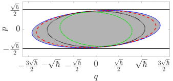
Figure 1: (Colour online) Various long-time states of the on-threshold OPO system in Eq. (24), represented by their 1-SD Wigner function contours in phase space, centred at the origin. The homodyne angles used by Alice and Bob ($\theta_{\text{o}}$, $\theta_{\text{u}}$) are at the black dot in Fig. 2. The unconditional state (solid black) shows infinite and finite variances in $q$ and $p$, respectively, as a result of the damping and squeezing. Alice’s filtered and smoothed states, are blue (filled grey) and dashed-red ellipses, respectively. The dotted-black ellipse shows the (pure) true state, conditioned on both Alice’s and Bob’s results, while the dot-dashed green ellipse shows the SWV “state.”

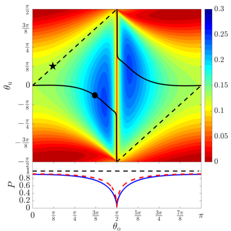
Figure 2: (Colour online) (Top) Contour plots of the RPR, Eq. (23), for the OPO system for different values of observed and unobserved homodyne phases using $\eta_{\text{o}}=0.5$. The dashed line represents $\theta_{\text{o}}=\theta_{\text{u}}$ and the solid line is the optimal $\theta_{\text{u}}$ (that giving the highest RPR for each value of $\theta_{\text{o}}$). The circle and the star relate to Figs. 1 and 3, respectively. (Bottom) Purity for the OPO’s filtered (solid blue) and smoothed (dashed red) states, choosing the optimal $\theta_{\text{u}}^{\rm opt}$ for each $\theta_{\text{o}}$.

The advantages LGQ state smoothing offers over filtering are readily seen in Fig. 1, where we note that the purity for a Gaussian state is defined as $P=(\hbar/2)\sqrt{|V|^{-1}}$ Wiseman and Milburn (2010) for a variance $V$. The smoothed state has a smaller variance (higher purity) than the filtered state, but has a larger variance than a pure state (purity less than unity). In contrast, the SWV state for the same system (i.e., using Eqs. (10)–(11)) is unphysical (its ellipse is smaller than that of a pure state).

Now that we have the closed-form expression for the smoothed LGQ state, we can investigate, in the steady state, some interesting limits in Alice’s measurement efficiency $\eta_{\text{o}}$, the fraction of the system output which is observed by Alice.

If, as in the OPO system we will consider later, the unconditioned ($\eta_{\text{o}}=0$) variance diverges, then Alice’s conditioned (filtered and retrofiltered) variances, if finite, must grow as $\eta_{\text{o}}\to 0$. From Eqs. (21)–(22), when $V_{\text{F}}$ and $V_{\text{R}}$ are large, compared to $V_{\text{T}}$, the smoothed LGQ state reduces to the SWV state Eqs. (10)–(11). The SWV state has the same form as classical smoothed states, which often have the same scaling as filtered states, but with a multiplicative constant improvement Tsang et al. (2009); Wheatley et al. (2010); Laverick et al. (2018). Consequently, in the limit $\eta_{\text{o}}\to 0$, we expect $P_{\rm SWV}=P_{\text{S}}\propto P_{\text{F}}$ as functions of $\eta_{\text{o}}$.

In the opposite limit, $\eta_{\text{o}}\to 1$, we analytically show Sup that the relative purity recovery (RPR),

$${\cal R}=\frac{P_{\text{S}}-P_{\text{F}}}{1-P_{\text{F}}}\,,$$ (23)

a measure of how much the purity is recovered from smoothing over filtering relative to the maximum recovery possible, usually scales with the unobserved efficiency. That is, ${\cal R}\propto\eta_{\text{u}}\equiv 1-\eta_{\text{o}}$.

Example of the on-threshold OPO system.— We now apply quantum state smoothing to the on-threshold OPO Wiseman and Milburn (2010); Wiseman and Doherty (2005), an LGQ system with $N=1$ described by the master equation

$$\hbar\dot{\rho}=-i[(\hat{q}\hat{p}+\hat{p}\hat{q})/2,\rho]+\mathcal{D}[\hat{q}+i\hat{p}]\rho\,.$$ (24)

The first term defines a Hamiltonian giving squeezing along the $p$-quadrature, while the second term describes the oscillator damping. Here, the drift and diffusion matrices are $A={\rm diag}(0,-2)$ and $D=\hbar I$. Let us assume that Alice observes the damping channel via homodyne detection. Therefore, the matrix $C_{\text{o}}$ in (12) is $C_{\text{o}}=2\sqrt{\eta_{\text{o}}/\hbar}\left(\cos\theta_{\text{o}},\sin\theta_{\text{o}}\right)$, where $\theta_{\text{o}}$ is the homodyne phase Wiseman and Milburn (2010); Wiseman and Doherty (2005). For simplicity, we assume Bob also performs a homodyne measurement, with a different phase $\theta_{\text{u}}$, so that $C_{\text{u}}=2\sqrt{\eta_{\text{u}}/\hbar}\left(\cos\theta_{\text{u}},\sin\theta_{\text{u}}\right)$. The measurement back-actions are described by matrices $\Gamma_{\rm r}=-\hbar C_{\rm r}/2$, for r $\in\{$o,u$\}$.

We now solve for filtered and smoothed states for the OPO in steady state. We are particularly interested in the RPR (23) of smoothing over filtering, and in the combinations of homodyne phases that result in the largest RPR. The RPR is always positive (see Fig. 2), meaning that the smoothed quantum state always has higher purity than the corresponding filtered one. If Alice’s phase $\theta_{\text{o}}$ is fixed, one might guess that Bob’s phase giving the best purity improvement should be the same, $\theta_{\text{u}}=\theta_{\text{o}}$. However, that is not at all true (see Fig. 2). The optimal $\theta_{\text{u}}^{\rm opt}$ is not a trivial function of $\theta_{\text{o}}$. Rather, $\theta_{\text{u}}^{\rm opt}\approx 0$, i.e., Bob should measure the $q$-quadrature, which is presumably related to the fact that, without measurement in, the variance in $q$ diverges.

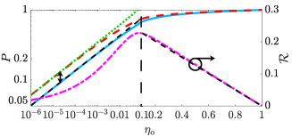
Figure 3: (Colour online) Purities, and the RPR, Eq. (23), at the starred point in Fig. 2, for the full range of Alice’s measurement efficiency $\eta_{\text{o}}$, with the lower efficiencies plotted on a log scale and the higher efficiencies on a linear scale, where the dashed vertical line at $\eta_{\text{o}}=0.1$ indicates the split. On both sides, we plot: purities of the filtered (solid blue), smoothed (dashed red) and the SWV (dotted green) states, all on a log scale (left-hand-side axis); and the RPR (${\cal R}$) (dot-dashed magenta), on a linear scale (the right-hand-side axis). For $\eta_{\text{o}}\to 0$, $P_{\text{F}}$ matches the simple analytic expression Sup $\sqrt{2|\cos\theta_{\text{o}}|}\eta_{\text{o}}^{1/4}$ (dashed black on left), and smoothing gives a factor of $\sqrt{2}$ improvement Sup , as shown by the small $\updownarrow$ symbol. For $\eta_{\text{o}}\to 1$, the RPR is $\propto(1-\eta_{\text{o}})$ (dashed black on right).

We then examine, in Fig. 3, the low and high efficiency limits for the OPO system at the starred point in Fig. 2. As predicted earlier, in the limit $\eta_{\text{o}}\to 0$ (left), the purities of the smoothed LGQ state and the SWV state are almost identical, and have a constant factor of improvement over that for filtering, as can be verified analytically Sup . However, $P_{\rm SWV}$ begins to separate from $P_{\text{S}}$ when the purities are no longer small, as the former proceeds to have purity greater than $1$ when $\eta_{\text{o}}>0.06$. In the limit $\eta_{\text{o}}\to 1$ (right), we see that the RPR has linear scaling in $\eta_{\text{u}}=1-\eta_{\text{o}}$, as expected. The approximation holds surprisingly well even when $\eta_{\text{u}}$ is not small.

To conclude, we have developed the theory of quantum state smoothing, which gives valid smoothed quantum states, for LGQ systems, a class of systems with wide physical applicability. By utilizing the Gaussian properties, we obtained closed-form smoothing solutions that do not require simulations of ensembles of unobserved measurement records and corresponding true states. This enabled us to perform detailed analysis of the smoothed quantum state for various measurement regimes. A question for future work is to understand the (numerically found) optimal strategy for greatest improvement in the purity. There are also interesting questions regarding how the smoothed LGQ variance (22) would react to inserting an invalid true state (i.e., one that does not solve Eq. (14)). Finally, we could compare the smoothed LGQ state to other state estimation techniques using future information, such as the most likely path approach in Refs. Chantasri et al. (2013); Weber et al. (2014).

We acknowledge the traditional owners of the land on which this work was undertaken at Griffith University, the Yuggera people. This research is funded by the Australian Research Council Centre of Excellence Program CE170100012. AC acknowledges the support of the Griffith University Postdoctoral Fellowship scheme.

Appendix A Haloed Filtering, Retrofiltering, and Smoothing

We begin by deriving the haloed filtering and retrofiltering equations, and then show that $V_{\text{F}}={\accentset{\raisebox{-1.0pt}{\scalebox{1.3}[0.4]{$\circ$}}}{V}}_{\text{F}}+V_{\text{T}}$ and $V_{\text{R}}={\accentset{\raisebox{-1.0pt}{\scalebox{1.3}[0.4]{$\circ$}}}{V}}_{\text{R}}-V_{\text{T}}$. We start with the equations for the true state (Eq. (13)-(14) in the main text) given both the observed and unobserved records,

$${\rm d}\langle{\hat{\bf x}}\rangle_{\text{T}}= A\langle{\hat{\bf x}}\rangle_{\text{T}}{\rm d}t+{\cal K}^{+}_{\text{o}}[V_{\text{T}}]{\rm d}{\bf w}_{\text{o}}+{\cal K}^{+}_{\text{u}}[V_{\text{T}}]{\rm d}{\bf w}_{\text{u}}\,,$$ (25)

$$\frac{{\rm d}V_{\text{T}}}{{\rm d}t}=A V_{\text{T}}+V_{\text{T}}A^{\top}+D-{\cal K}^{+}_{\text{o}}[V_{\text{T}}]{\cal K}^{+}_{\text{o}}[V_{\text{T}}]^{\top}-{\cal K}^{+}_{\text{u}}[V_{\text{T}}]{\cal K}^{+}_{\text{u}}[V_{\text{T}}]^{\top}\,.$$ (26)

We then use $\accentset{\raisebox{-1.0pt}{\scalebox{1.3}[0.4]{$\circ$}}}{{\bf x}}=\langle{\hat{\bf x}}\rangle_{\text{T}}$ and define $\accentset{\raisebox{-1.0pt}{\scalebox{1.3}[0.4]{$\circ$}}}{E}{\rm d}\accentset{\raisebox{-1.0pt}{\scalebox{1.3}[0.4]{$\circ$}}}{{\bf v}}_{\text{p}}={\cal K}^{+}_{\text{o}}[V_{\text{T}}]{\rm d}{\bf w}_{\text{o}}+{\cal K}^{+}_{\text{u}}[V_{\text{T}}]{\rm d}{\bf w}_{\text{u}}$, so that Eq. (25) is recast in a simple form as

$${\rm d}\accentset{\raisebox{-1.0pt}{\scalebox{1.3}[0.4]{$\circ$}}}{{\bf x}}=A\accentset{\raisebox{-1.0pt}{\scalebox{1.3}[0.4]{$\circ$}}}{{\bf x}}{\rm d}t+\accentset{\raisebox{-1.0pt}{\scalebox{1.3}[0.4]{$\circ$}}}{E}{\rm d}\accentset{\raisebox{-1.0pt}{\scalebox{1.3}[0.4]{$\circ$}}}{{\bf v}}_{\text{p}}\,.$$ (27)

That is, Eq. (27) has the same form as the classical linear Langevin equation (Eq. (2) in the main text) and $\accentset{\raisebox{-1.0pt}{\scalebox{1.3}[0.4]{$\circ$}}}{{\bf x}}$ can be considered a classical parameter (a possible trajectory of the centroid of the true state). Moreover, Alice’s observed measurement current (Eq. (12) in the main text),

$${\bf y}_{\text{o}}{\rm d}t=C_{\text{o}}\accentset{\raisebox{-1.0pt}{\scalebox{1.3}[0.4]{$\circ$}}}{{\bf x}}{\rm d}t+{\rm d}{\bf w}_{\text{o}}\,,$$ (28)

has the same form as Eq. (4) in the main text, with ${\rm d}{\bf w}_{\text{o}}$ identified as ${\rm d}\accentset{\raisebox{-1.0pt}{\scalebox{1.3}[0.4]{$\circ$}}}{{\bf v}}_{\text{m}}$. The correlation of the measurement noise with the process noise is easily evaluated as

$$\accentset{\raisebox{-1.0pt}{\scalebox{1.3}[0.4]{$\circ$}}}{\Gamma}^{\top}{\rm d}t=\accentset{\raisebox{-1.0pt}{\scalebox{1.3}[0.4]{$\circ$}}}{E}{\rm d}\accentset{\raisebox{-1.0pt}{\scalebox{1.3}[0.4]{$\circ$}}}{{\bf v}}_{\text{p}}({\rm d}\accentset{\raisebox{-1.0pt}{\scalebox{1.3}[0.4]{$\circ$}}}{{\bf v}}_{\text{m}})^{\top}={\cal K}^{+}_{\text{o}}[V_{\text{T}}]{\rm d}t.$$ (29)

That is, $\accentset{\raisebox{-1.0pt}{\scalebox{1.3}[0.4]{$\circ$}}}{\Gamma}=\Gamma_{\rm o}+C_{\rm o}V_{\text{T}}$. Similarly, we can define

$$\accentset{\raisebox{-1.0pt}{\scalebox{1.3}[0.4]{$\circ$}}}{D}=\accentset{\raisebox{-1.0pt}{\scalebox{1.3}[0.4]{$\circ$}}}{E}\accentset{\raisebox{-1.0pt}{\scalebox{1.3}[0.4]{$\circ$}}}{E}^{\top}={\cal K}^{+}_{\text{o}}[V_{\text{T}}]{\cal K}^{+}_{\text{o}}[V_{\text{T}}]^{\top}+{\cal K}^{+}_{\text{u}}[V_{\text{T}}]{\cal K}^{+}_{\text{u}}[V_{\text{T}}]^{\top}.$$ (30)

A.1 Filtering

From the above, we obtain the haloed filtering equations in a similar way using Eqs. (6)–(7) in the main text, replacing ${\bf x}$, $D$, $C$, and $\Gamma$ with $\accentset{\raisebox{-1.0pt}{\scalebox{1.3}[0.4]{$\circ$}}}{{\bf x}}$, $\accentset{\raisebox{-1.0pt}{\scalebox{1.3}[0.4]{$\circ$}}}{D}$, $C_{\text{o}}$, and $\accentset{\raisebox{-1.0pt}{\scalebox{1.3}[0.4]{$\circ$}}}{\Gamma}$, respectively. The haloed filtering equations are then given by

$${\rm d}\langle{\accentset{\raisebox{-1.0pt}{\scalebox{1.3}[0.4]{$\circ$}}}{{\bf x}}}\rangle_{\text{F}}=A\langle{\accentset{\raisebox{-1.0pt}{\scalebox{1.3}[0.4]{$\circ$}}}{{\bf x}}}\rangle_{\text{F}}{\rm d}t+{\cal K}^{+}_{\text{o}}[{\accentset{\raisebox{-1.0pt}{\scalebox{1.3}[0.4]{$\circ$}}}{V}}_{\text{F}}+V_{\text{T}}]{\rm d}\accentset{\raisebox{-1.0pt}{\scalebox{1.3}[0.4]{$\circ$}}}{{\bf w}}_{\text{F}}\,,$$ (31)

$$\frac{{\rm d}{\accentset{\raisebox{-1.0pt}{\scalebox{1.3}[0.4]{$\circ$}}}{V}}_{\text{F}}}{{\rm d}t}=A{\accentset{\raisebox{-1.0pt}{\scalebox{1.3}[0.4]{$\circ$}}}{V}}_{\text{F}}+{\accentset{\raisebox{-1.0pt}{\scalebox{1.3}[0.4]{$\circ$}}}{V}}_{\text{F}}A^{\top}+\accentset{\raisebox{-1.0pt}{\scalebox{1.3}[0.4]{$\circ$}}}{D}-{\cal K}^{+}_{\text{o}}[{\accentset{\raisebox{-1.0pt}{\scalebox{1.3}[0.4]{$\circ$}}}{V}}_{\text{F}}+V_{\text{T}}]{\cal K}^{+}_{\text{o}}[{\accentset{\raisebox{-1.0pt}{\scalebox{1.3}[0.4]{$\circ$}}}{V}}_{\text{F}}+V_{\text{T}}]^{\top}\,,$$ (32)

as shown in Eqs. (17)–(18) of the main text, where ${\rm d}\accentset{\raisebox{-1.0pt}{\scalebox{1.3}[0.4]{$\circ$}}}{{\bf w}}_{\text{F}}\equiv{\bf y}_{\text{o}}{\rm d}t-C_{\text{o}}\langle{\accentset{\raisebox{-1.0pt}{\scalebox{1.3}[0.4]{$\circ$}}}{{\bf x}}}\rangle_{\text{F}}{\rm d}t$.

To show the relation between the haloed filtering equation and the usual quantum filtering equations, we begin by recognising a different form of $\accentset{\raisebox{-1.0pt}{\scalebox{1.3}[0.4]{$\circ$}}}{D}$. From Eq. (26) we see that

$$\accentset{\raisebox{-1.0pt}{\scalebox{1.3}[0.4]{$\circ$}}}{D}=AV_{\text{T}}+V_{\text{T}}A^{\top}+D-\frac{{\rm d}V_{\text{T}}}{{\rm d}t}\,,$$ (33)

and substituting this into Eq. (32) to get

$$\frac{{\rm d}}{{\rm d}t}({\accentset{\raisebox{-1.0pt}{\scalebox{1.3}[0.4]{$\circ$}}}{V}}_{\text{F}}+V_{\text{T}})=A({\accentset{\raisebox{-1.0pt}{\scalebox{1.3}[0.4]{$\circ$}}}{V}}_{\text{F}}+V_{\text{T}})+({\accentset{\raisebox{-1.0pt}{\scalebox{1.3}[0.4]{$\circ$}}}{V}}_{\text{F}}+V_{\text{T}})A^{\top}+D-{\cal K}^{+}_{\text{o}}[{\accentset{\raisebox{-1.0pt}{\scalebox{1.3}[0.4]{$\circ$}}}{V}}_{\text{F}}+V_{\text{T}}]{\cal K}^{+}_{\text{o}}[{\accentset{\raisebox{-1.0pt}{\scalebox{1.3}[0.4]{$\circ$}}}{V}}_{\text{F}}+V_{\text{T}}]\,.$$ (34)

If we use $V_{\text{F}}={\accentset{\raisebox{-1.0pt}{\scalebox{1.3}[0.4]{$\circ$}}}{V}}_{\text{F}}+V_{\text{T}}$ in the above equation, we obtain exactly Eq. (7) in the main text, i.e., an equation for the filtered variance. Therefore, we can regard this variance $V_{\text{F}}$ as the variance of the usual filtering for an LGQ system, which one could derive without the Alice-Bob protocol. We can also check that the haloed filtered mean is identical to the usual filtered mean (Eq. (6) of the main text, but for an LGQ system), as should be the case from the convolution. This can be seen by using $V_{\text{F}}={\accentset{\raisebox{-1.0pt}{\scalebox{1.3}[0.4]{$\circ$}}}{V}}_{\text{F}}+V_{\text{T}}$ in the haloed filtered estimate Eq. (31), which gives

$${\rm d}\langle{\accentset{\raisebox{-1.0pt}{\scalebox{1.3}[0.4]{$\circ$}}}{{\bf x}}}\rangle_{\text{F}}=A\langle{\accentset{\raisebox{-1.0pt}{\scalebox{1.3}[0.4]{$\circ$}}}{{\bf x}}}\rangle_{\text{F}}{\rm d}t+{\cal K}^{+}_{\text{o}}[V_{\text{F}}]{\rm d}\accentset{\raisebox{-1.0pt}{\scalebox{1.3}[0.4]{$\circ$}}}{{\bf w}}_{\text{F}}\,.$$ (35)

Considering the same initial conditions for $\langle{\accentset{\raisebox{-1.0pt}{\scalebox{1.3}[0.4]{$\circ$}}}{{\bf x}}}\rangle_{\text{F}}$ and $\langle{\hat{\bf x}}\rangle_{\text{F}}$, the haloed filtered mean will remain identical to the filtered mean, $\langle{\hat{\bf x}}\rangle_{\text{F}}=\langle{\accentset{\raisebox{-1.0pt}{\scalebox{1.3}[0.4]{$\circ$}}}{{\bf x}}}\rangle_{\text{F}}$, so the innovations will also be identical, with ${\rm d}\accentset{\raisebox{-1.0pt}{\scalebox{1.3}[0.4]{$\circ$}}}{{\bf w}}_{\text{F}}={\rm d}{\bf w}_{\text{F}}\equiv{\bf y}_{\text{o}}{\rm d}t-C_{\text{o}}\langle{\hat{\bf x}}\rangle_{\text{F}}$. Note that neither of these innovations is the same as the ${\rm d}{\bf w}_{\text{o}}={\bf y}_{\text{o}}{\rm d}t-C_{\text{o}}\langle{\hat{\bf x}}\rangle_{\text{T}}$ in Eq. (25), as the latter is the innovation in Alice’s record defined using the true state, i.e., from Bob’s all-knowing point of view rather than Alice’s.

A.2 Retrofiltering and Smoothing

Similarly to the filtering case, we can get the haloed retrofiltering equations using Eqs. (8)–(9) in the main text

$$-{\rm d}\langle{\accentset{\raisebox{-1.0pt}{\scalebox{1.3}[0.4]{$\circ$}}}{{\bf x}}}\rangle_{\text{R}} =-A\langle{\accentset{\raisebox{-1.0pt}{\scalebox{1.3}[0.4]{$\circ$}}}{{\bf x}}}\rangle_{\text{R}}{\rm d}t+{\cal K}^{-}_{\text{o}}[{\accentset{\raisebox{-1.0pt}{\scalebox{1.3}[0.4]{$\circ$}}}{V}}_{\text{R}}-V_{\text{T}}]{\rm d}\accentset{\raisebox{-1.0pt}{\scalebox{1.3}[0.4]{$\circ$}}}{{\bf w}}_{\text{R}}\,,$$ (36)

$$-\frac{{\rm d}{\accentset{\raisebox{-1.0pt}{\scalebox{1.3}[0.4]{$\circ$}}}{V}}_{\text{R}}}{{\rm d}t} =-A{\accentset{\raisebox{-1.0pt}{\scalebox{1.3}[0.4]{$\circ$}}}{V}}_{\text{R}}-{\accentset{\raisebox{-1.0pt}{\scalebox{1.3}[0.4]{$\circ$}}}{V}}_{\text{R}}A^{\top}+\accentset{\raisebox{-1.0pt}{\scalebox{1.3}[0.4]{$\circ$}}}{D}-{\cal K}^{-}_{\text{o}}[{\accentset{\raisebox{-1.0pt}{\scalebox{1.3}[0.4]{$\circ$}}}{V}}_{\text{R}}-V_{\text{T}}]{\cal K}^{-}_{\text{o}}[{\accentset{\raisebox{-1.0pt}{\scalebox{1.3}[0.4]{$\circ$}}}{V}}_{\text{R}}-V_{\text{T}}]\,,$$ (37)

where ${\rm d}\accentset{\raisebox{-1.0pt}{\scalebox{1.3}[0.4]{$\circ$}}}{{\bf w}}_{\text{R}}\equiv{\bf y}_{\text{o}}{\rm d}t-C_{\text{o}}\langle{\accentset{\raisebox{-1.0pt}{\scalebox{1.3}[0.4]{$\circ$}}}{{\bf x}}}\rangle_{\text{R}}$. Now, adding Eq. (33) to Eq. (37), we arrive at

$$-\frac{{\rm d}}{{\rm d}t}({\accentset{\raisebox{-1.0pt}{\scalebox{1.3}[0.4]{$\circ$}}}{V}}_{\text{R}}-V_{\text{T}})=-A({\accentset{\raisebox{-1.0pt}{\scalebox{1.3}[0.4]{$\circ$}}}{V}}_{\text{R}}-V_{\text{T}})-({\accentset{\raisebox{-1.0pt}{\scalebox{1.3}[0.4]{$\circ$}}}{V}}_{\text{R}}-V_{\text{T}})A^{\top}+D-{\cal K}^{-}_{\text{o}}[{\accentset{\raisebox{-1.0pt}{\scalebox{1.3}[0.4]{$\circ$}}}{V}}_{\text{R}}-V_{\text{T}}]{\cal K}^{-}_{\text{o}}[{\accentset{\raisebox{-1.0pt}{\scalebox{1.3}[0.4]{$\circ$}}}{V}}_{\text{R}}-V_{\text{T}}]\,,$$ (38)

which is the equation for the retrofiltered variance $V_{\text{R}}$ and as a result we have $V_{\text{R}}={\accentset{\raisebox{-1.0pt}{\scalebox{1.3}[0.4]{$\circ$}}}{V}}_{\text{R}}-V_{\text{T}}$.

The relation $V_{\text{R}}={\accentset{\raisebox{-1.0pt}{\scalebox{1.3}[0.4]{$\circ$}}}{V}}_{\text{R}}-V_{\text{T}}$ is interesting, as it shows the asymmetry between the filtered state and the retrofiltered effect. Note that $V_{R}$ is not the variance for a state conditioned only on the future observed record. Rather it is the variance of a POVM element for the future record. To obtain $V_{\text{R}}$ in general it will be easier to compute the inverse of ${\accentset{\raisebox{-1.0pt}{\scalebox{1.3}[0.4]{$\circ$}}}{V}}_{\text{R}}$, rather than ${\accentset{\raisebox{-1.0pt}{\scalebox{1.3}[0.4]{$\circ$}}}{V}}_{\text{R}}$ itself, for calculating the smoothed state. This is because the final condition on the retrofiltered variance (haloed or not) is often taken to be infinite, as mentioned in the main text. Defining the inverse $\accentset{\raisebox{-1.0pt}{\scalebox{1.3}[0.4]{$\circ$}}}{\Lambda}_{\text{R}}={\accentset{\raisebox{-1.0pt}{\scalebox{1.3}[0.4]{$\circ$}}}{V}}_{\text{R}}^{-1}$, we use the relation $\frac{{\rm d}}{{\rm d}t}\left({\accentset{\raisebox{-1.0pt}{\scalebox{1.3}[0.4]{$\circ$}}}{V}}_{\text{R}}{\accentset{\raisebox{-1.0pt}{\scalebox{1.3}[0.4]{$\circ$}}}{\Lambda}}_{\text{R}}\right)=0$ to get

$$\frac{{\rm d}{\accentset{\raisebox{-1.0pt}{\scalebox{1.3}[0.4]{$\circ$}}}{\Lambda}}_{\text{R}}}{{\rm d}t}=-{\accentset{\raisebox{-1.0pt}{\scalebox{1.3}[0.4]{$\circ$}}}{\Lambda}}_{\text{R}}\frac{{\rm d}{\accentset{\raisebox{-1.0pt}{\scalebox{1.3}[0.4]{$\circ$}}}{V}}_{\text{R}}}{{\rm d}t}{\accentset{\raisebox{-1.0pt}{\scalebox{1.3}[0.4]{$\circ$}}}{\Lambda}}_{\text{R}}\,.$$ (39)

From this we obtain

$$-\frac{{\rm d}{\accentset{\raisebox{-1.0pt}{\scalebox{1.3}[0.4]{$\circ$}}}{\Lambda}}_{\text{R}}}{{\rm d}t}=\bar{A}{\accentset{\raisebox{-1.0pt}{\scalebox{1.3}[0.4]{$\circ$}}}{\Lambda}}_{\text{R}}+{\accentset{\raisebox{-1.0pt}{\scalebox{1.3}[0.4]{$\circ$}}}{\Lambda}}_{\text{R}}\bar{A}^{\top}-{\accentset{\raisebox{-1.0pt}{\scalebox{1.3}[0.4]{$\circ$}}}{\Lambda}}_{\text{R}}\bar{D}{\accentset{\raisebox{-1.0pt}{\scalebox{1.3}[0.4]{$\circ$}}}{\Lambda}}_{\text{R}}+C_{\text{o}}^{\top}C_{\text{o}}\,,$$ (40)

with $\bar{A}=A-\Gamma_{\text{o}}C_{\text{o}}-V_{\text{T}}C_{\text{o}}^{\top}C_{\text{o}}$ and $\bar{D}=\accentset{\raisebox{-1.0pt}{\scalebox{1.3}[0.4]{$\circ$}}}{D}-\Gamma_{\text{o}}^{\top}\Gamma_{\text{o}}-\Gamma_{\text{o}}^{\top}C_{\text{o}}V_{\text{T}}-V_{\text{T}}C_{\text{o}}^{\top}\Gamma_{\text{o}}-V_{\text{T}}C_{\text{o}}^{\top}C_{\text{o}}V_{\text{T}}$. This way, the final condition is ${\accentset{\raisebox{-1.0pt}{\scalebox{1.3}[0.4]{$\circ$}}}{\Lambda}}_{\text{R}}(T)=0$ and the LGQ smoothed state in terms of ${\accentset{\raisebox{-1.0pt}{\scalebox{1.3}[0.4]{$\circ$}}}{\Lambda}}_{\text{R}}$ and $V_{\text{F}}$ is given by

$$\langle{\accentset{\raisebox{-1.0pt}{\scalebox{1.3}[0.4]{$\circ$}}}{{\bf x}}}\rangle_{\rm S}=(V_{\text{S}}-V_{\text{T}})[(V_{\text{F}}-V_{\text{T}})^{-1}\langle{\accentset{\raisebox{-1.0pt}{\scalebox{1.3}[0.4]{$\circ$}}}{{\bf x}}}\rangle_{\text{F}}+{\accentset{\raisebox{-1.0pt}{\scalebox{1.3}[0.4]{$\circ$}}}{\Lambda}}_{\text{R}}\langle{\accentset{\raisebox{-1.0pt}{\scalebox{1.3}[0.4]{$\circ$}}}{{\bf x}}}\rangle_{\text{R}}]\,,$$ (41)

$$V_{\text{S}}=\left[(V_{\text{F}}-V_{\text{T}})^{-1}+{\accentset{\raisebox{-1.0pt}{\scalebox{1.3}[0.4]{$\circ$}}}{\Lambda}}_{\text{R}}\right]^{-1}+V_{\text{T}}\,.$$ (42)

Appendix B Purities and RPR for different efficiency limits

B.1 Low Efficiency Limit

For the low efficiency limit, specifically for the on-threshold OPO system, we will show here that the purity $P_{\rm C}\propto\eta_{\text{o}}^{1/4}$, where ${\rm C}\in\{{\rm F},{\rm SWV}\}$. We first consider the case $\eta_{\text{o}}=0$, i.e., no conditioning on measurement results, where the linear matrix equation for the steady state of the filtered variance $V_{\text{F}}$ is given by

$$AV_{\text{F}}+V_{\text{F}}A^{\top}+D=0\,,$$ (43)

with $A={\rm diag}(0,-2)$ and $D=\hbar I$. Since the matrix $A$ for this case is not strictly stable (with one of its eigenvalues being zero), there is no stationary matrix solution for (43), but in a long-time limit, we have Wiseman and Milburn (2010)

$$V_{\text{F}}\to\frac{\hbar}{2}\left[\begin{array}[]{ccccc}\infty&0\\ 0&1/2\\ \end{array}\right].$$ (44)

We then consider the low efficiency case, for a small but non-zero observed efficiency $\eta_{\rm o}\rightarrow 0$. Now the filtered variance is given by Eq. (7) in the main text. This equation leads to the variance in the $q$-quadrature (top-left element of the variance matrix) becoming finite, as long as the homodyne current contains some information about this quadrature ($\theta_{\text{o}}\neq\pm\pi/2$). Explicitly, if we consider an arbitrary $V_{F}$ of the form

$$V_{\text{F}}=\frac{\hbar}{2}\left[\begin{array}[]{cc}\alpha_{\text{F}}&\beta_{\text{F}}\\ \beta_{\text{F}}&\gamma_{\text{F}}\\ \end{array}\right]\,,$$ (45)

we can obtain three relations for $\alpha_{\text{F}}$, $\beta_{\text{F}}$ and $\gamma_{\text{F}}$, using Eq. (7) (in the main text) and the matrices $C_{\rm o}$, $\Gamma_{\rm o}$ for the OPO system defined there:

$$1 =\eta_{\text{o}}\left[(\alpha_{\text{F}}-1)\cos\theta_{\text{o}}+\beta_{\text{F}}\sin\theta_{\text{o}}\right]^{2},$$ (46)

$$-\beta_{\text{F}} =\eta_{\text{o}}\left((\alpha_{\text{F}}-1)\cos\theta_{\text{o}}+\beta_{\text{F}}\sin\theta_{\text{o}}\right)\left(\beta_{\text{F}}\cos\theta_{\text{o}}+(\gamma_{\text{F}}-1)\sin\theta_{\text{o}}\right),$$ (47)

$$1-2\gamma_{\text{F}} =\eta_{\text{o}}\left[\beta_{\text{F}}\cos\theta_{\text{o}}+(\gamma_{\text{F}}-1)\sin\theta_{\text{o}}\right]^{2}.$$ (48)

To evaluate the purity of the filtered LGQ state, $P_{\text{F}}$, in the low efficiency limit, we do not need to solve for the full solution of $V_{\text{F}}$ from the above equations. The major contribution the measurement has to the variance is to bring the $q$-component, that is the top-left element, $\alpha_{\text{F}}$, from infinity to a large but finite value; whereas the $\gamma_{\text{F}}$ and $\beta_{\text{F}}$ elements, describing variance in $p$-quadrature and covariance between the two quadratures, should still have values closed to those of the unconditional solution since they are finite even in the absence of any information, and the small amount of information in the low efficiency limit will make little difference. Consequently, we can treat $\alpha_{\text{F}}$ as being much larger than $\gamma_{\text{F}}$ and $\beta_{\text{F}}$, where the former scales as an inverse order of $\eta_{\text{o}}$ and the latter two are $O(\eta_{\text{o}}^{k})$ for $k\geq 0$. From this, we can only use (46) and solve for $\alpha_{\text{F}}$ to leading order in $\eta_{\text{o}}$, giving

$$\alpha_{\text{F}}\approx|\cos\theta_{\text{o}}|^{-1}\eta_{\text{o}}^{-1/2}\,.\\$$ (49)

We now calculate the filtered purity using an assumption that the variance in $p$-quadrature represented by $\gamma_{\text{F}}$ should still stay close to its unconditional value $1/2$, beginning with

$$|V_{\text{F}}| \approx|2\cos\theta_{\text{o}}|^{-1}\eta_{\text{o}}^{-1/2}-\beta_{\text{F}}^{2}\approx|2\cos\theta_{\text{o}}|^{-1}\eta_{\text{o}}^{-1/2}\,.$$ (50)

Thus we get

$$P_{\text{F}} =\frac{\hbar}{2}\sqrt{|V_{\text{F}}|^{-1}}=\sqrt{2|\cos\theta_{\text{o}}|}\,\eta_{\text{o}}^{1/4}\,,$$ (51)

where we can see the $\eta_{\text{o}}^{1/4}$ scaling.

For the purity of the smoothed weak-valued state $P_{\rm SWV}$ in the small efficiency limit, we can use the intuition that the information used in the classical smoothing is twice as much in the filtering (considering the steady-state case), which should result in reducing the large variance in $q$-quadrature by half, i.e., $\alpha_{\rm SWV}\approx\frac{1}{2}\alpha_{\text{F}}$, still much larger than $\beta_{\rm SWV}$ and $\gamma_{\rm SWV}$. As in the filtered case, we expect the latter two to remain little changed from their unconditioned values. Thus $|V_{\rm SWV}|\approx|4\cos\theta_{\text{o}}|^{-1}\eta_{\text{o}}^{-1/2}$ and

$$P_{\rm SWV} =\frac{\hbar}{2}\sqrt{|V_{\rm SWV}^{-1}|}\approx 2\sqrt{|\cos\theta_{\text{o}}|}\,\eta_{\text{o}}^{1/4}\,,$$ (52)

where we see the constant factor of improvement $\sqrt{2}$ over filtering.

We now rigorously check our intuition by finding the exact solutions for both $P_{\text{F}}$ and $P_{\rm SWV}$ in this limit, $\eta_{\text{o}}\to 0$. Solving the full coupled equations (46)-(48), we obtain $V_{\text{F}}$ and $P_{\text{F}}$ to leading orders in $\eta_{\text{o}}$,

$$V_{\text{F}}=\frac{\hbar}{2}\left[\begin{array}[]{cc}|\sec\theta_{\text{o}}|\eta_{\text{o}}^{-1/2}&\frac{1}{2}|\sin\theta_{\text{o}}|\eta_{\text{o}}^{1/2}\\ \frac{1}{2}|\sin\theta_{\text{o}}|\eta_{\text{o}}^{1/2}&1/2\\ \end{array}\right]\,,\qquad P_{\text{F}}=\sqrt{2|\cos\theta_{\text{o}}|}\,\eta_{\text{o}}^{1/4}\,,$$ (53)

as expected. For the $V_{\rm SWV}$, we first need to calculate the retrofiltered variance $V_{\text{R}}$. We solve for the full solution of $V_{\text{R}}$ from Eq. (9) in the main text (in the steady-state limit) to leading orders in $\eta_{\text{o}}$,

$$V_{\text{R}}=\frac{\hbar}{2}\left[\begin{array}[]{cc}|\sec\theta_{\text{o}}|\eta_{\text{o}}^{-1/2}&2|\csc\theta_{\text{o}}|\eta_{\text{o}}^{-1/2}\\ 2|\csc\theta_{\text{o}}|\eta_{\text{o}}^{-1/2}&2|\csc\theta_{\text{o}}|^{2}\eta_{\text{o}}^{-1}\\ \end{array}\right]\,.$$ (54)

Finally, we can calculate the SWV variance (using Eq. (11) in the main text) and its purity, arriving at

$$V_{\rm SWV}=\frac{\hbar}{2}\left[\begin{array}[]{cc}\frac{1}{2}|\sec\theta_{\text{o}}|\eta_{\text{o}}^{-1/2}&\frac{1}{2}|\sin\theta_{\text{o}}|\eta_{\text{o}}^{1/2}\\ \frac{1}{2}|\sin\theta_{\text{o}}|\eta_{\text{o}}^{1/2}&1/2\\ \end{array}\right]\,,\qquad P_{\rm SWV}=2\sqrt{|\cos\theta_{\text{o}}|}\eta_{\text{o}}^{1/4}\,,$$ (55)

which are consistent with our intuitive approach.

B.2 High Efficiency Limit

In this section we derive the $\eta_{\text{u}}$ scaling for the steady-state relative purity recovery (RPR) in the high efficiency limit for Alice ($\eta_{\text{o}}\to 1$), in general cases, not only for the OPO system. We first point out that with $\eta_{\text{o}}=1$ (all available records are observed), the filtered and true variances are equal. So, if we express the filtered variance as $V_{\text{F}}=V_{\text{T}}+Q$, it will typically be the case that $Q\to 0$ as $\eta_{\text{o}}\to 1$, and we assume this to be so in all that follows. In this limit, we can see that the variance of the smoothed state, Eq. (42), is

$$V_{\text{S}} =\left[Q^{-1}+{\accentset{\raisebox{-1.0pt}{\scalebox{1.3}[0.4]{$\circ$}}}{\Lambda}}_{\text{R}}\right]^{-1}+V_{\text{T}}$$ (56)

$$=Q\left[1+{\accentset{\raisebox{-1.0pt}{\scalebox{1.3}[0.4]{$\circ$}}}{\Lambda}}_{\text{R}}Q\right]^{-1}+V_{\text{T}}$$ (57)

$$\approx Q\left[1-{\accentset{\raisebox{-1.0pt}{\scalebox{1.3}[0.4]{$\circ$}}}{\Lambda}}_{\text{R}}Q\right]+V_{\text{T}}$$ (58)

$$=V_{\text{F}}-Q{\accentset{\raisebox{-1.0pt}{\scalebox{1.3}[0.4]{$\circ$}}}{\Lambda}}_{\text{R}}Q\,,$$ (59)

where the approximation holds since $Q$ is small. This nicely shows how information from the future, as expressed by ${\accentset{\raisebox{-1.0pt}{\scalebox{1.3}[0.4]{$\circ$}}}{\Lambda}}_{\text{R}}\neq 0$, makes the smoothed variance smaller than the filtered one.

Now we show that the RPR (Eq. (23) of the main text) scales as $O(Q)$. The purity of a LGQ state is given by

$$P_{\rm C}=\frac{\hbar}{2}\left[\sqrt{|V_{\rm C}|}\right]^{-1}\,,$$ (60)

for ${\rm C}={\rm F,S}$ or ${\rm T}$. The purity of the filtered state in the high efficiency limit is

$$P_{\text{F}} =\frac{\hbar}{2}\left[\sqrt{|V_{\text{T}}+Q|}\right]^{-1},$$ (61)

$$=\frac{\hbar}{2\sqrt{|V_{\text{T}}|}}\left[\sqrt{|I+V_{\text{T}}^{-1}Q|}\right]^{-1},$$ (62)

$$=P_{\text{T}}\left[\sqrt{|I+V_{\text{T}}^{-1}Q|}\right]^{-1}\,.$$ (63)

Now we need to evaluate $|I+Y|$, where $Y=V_{\text{T}}^{-1}Q$ is small. Using the formula $|e^{Y}|=\exp[{\rm Tr}(Y)]$ Hall (2015) and expanding the left and right exponential terms, we get, to leading order

$$|I+Y|\approx 1+{\rm Tr}(Y)\,.$$ (64)

The purity of the filtered state is thus given by

$$P_{\text{F}} \approx P_{\text{T}}\left[\sqrt{1+{\rm Tr}(V_{\text{T}}^{-1}Q)}\right]^{-1}$$ (65)

$$\approx P_{\text{T}}\left[1-{\rm Tr}\left(V_{\text{T}}^{-1}Q\right)/2\right]\,.$$ (66)

For the purity of the smoothed state, we express the smoothed variance as $V_{\text{S}}=V_{\text{F}}-X$, where $X=Q\accentset{\raisebox{-1.0pt}{\scalebox{1.3}[0.4]{$\circ$}}}{\Lambda}_{\text{R}}Q$. Following the similar derivation as for the purity of the filtered state, we obtain the purity of the smoothed state as $P_{\text{S}}\approx P_{\text{F}}\left[1+{\rm Tr}\left(V_{\text{F}}^{-1}Q\accentset{\raisebox{-1.0pt}{\scalebox{1.3}[0.4]{$\circ$}}}{\Lambda}_{\text{R}}Q\right)/2\right]$. The RPR is then given by

$${\cal R} =\frac{P_{\text{S}}-P_{\text{F}}}{1-P_{\text{F}}}$$ (67)

$$=\frac{P_{\text{F}}+P_{\text{F}}{\rm Tr}\left(V_{\text{F}}^{-1}Q\accentset{\raisebox{-1.0pt}{\scalebox{1.3}[0.4]{$\circ$}}}{\Lambda}_{\text{R}}Q\right)/2-P_{\text{F}}}{1-P_{\text{T}}+P_{\text{T}}{\rm Tr}\left(V_{\text{T}}^{-1}Q)\right)/2}$$ (68)

$$=\frac{P_{\text{F}}{\rm Tr}\left(V_{\text{F}}^{-1}Q\accentset{\raisebox{-1.0pt}{\scalebox{1.3}[0.4]{$\circ$}}}{\Lambda}_{\text{R}}Q\right)/2}{1-P_{\text{T}}+P_{\text{T}}{\rm Tr}\left(V_{\text{T}}^{-1}Q)\right)/2}\,.$$ (69)

If we consider that Bob observes the part unobserved by Alice’s measurement, i.e., $\eta_{\text{u}}=1-\eta_{\text{o}}$, the true state will be a pure state ($P_{\text{T}}=1$), as it is conditioned on all possible measurement records. The RPR then becomes

$${\cal R} \approx P_{\text{F}}\frac{{\rm Tr}\left((V_{\text{T}}+Q)^{-1}Q\accentset{\raisebox{-1.0pt}{\scalebox{1.3}[0.4]{$\circ$}}}{\Lambda}_{\text{R}}Q\right)}{{\rm Tr}\left(V_{\text{T}}^{-1}Q\right)}$$ (70)

$$\approx P_{\text{F}}\frac{{\rm Tr}\left[\left(V_{\text{T}}^{-1}-V_{\text{T}}^{-1}QV_{\text{T}}^{-1}\right)Q\accentset{\raisebox{-1.0pt}{\scalebox{1.3}[0.4]{$\circ$}}}{\Lambda}_{\text{R}}Q\right]}{{\rm Tr}\left(V_{\text{T}}^{-1}Q\right)}$$ (71)

$$\approx P_{\text{F}}\frac{{\rm Tr}\left(V_{\text{T}}^{-1}Q\accentset{\raisebox{-1.0pt}{\scalebox{1.3}[0.4]{$\circ$}}}{\Lambda}_{\text{R}}Q\right)}{{\rm Tr}\left(V_{\text{T}}^{-1}Q\right)}$$ (72)

$$=\frac{O(Q^{2})}{O(Q)}=O(Q)\,.$$ (73)

Finally, all that is left is to check how $Q$ scales with the unobserved measurement efficiency $\eta_{\text{u}}$. Substituting in $V_{\text{F}}=V_{\text{T}}+Q$ into Eq. (7) in the main text, we obtain

$$0=A(V_{\text{T}}+Q)+(V_{\text{T}}+Q)A^{\top}+D-{\cal K}^{+}_{\text{o}}[V_{\text{T}}+Q]{\cal K}^{+}_{\text{o}}[V_{\text{T}}+Q]^{\top}\,,$$ (74)

considering the system to be in the steady state. Rearranging the above terms and using Eq. (14) in the main text (also in the steady state), we arrive at

$$-\bar{A}Q-Q\bar{A}^{\top}+Q{C}_{\text{o}}^{\top}{C}_{\text{o}}Q=\eta_{\text{u}}\bar{\cal K}^{+}_{\text{u}}[V_{\text{T}}]\bar{\cal K}^{+}_{\text{u}}[V_{\text{T}}]^{\top}\,,$$ (75)

where we are using $\bar{A}=A-\Gamma_{\text{o}}^{\top}C_{\text{o}}-V_{\text{T}}{C}^{\top}_{\text{o}}{C}_{\text{o}}$ as in Sec. I B above, and we have defined $\bar{\cal K}^{+}_{\rm r}[V]=\sqrt{1/\eta_{\text{u}}}{\cal K}^{+}_{\text{u}}[V]$ so that in the limit $\eta_{\text{u}}\to 0$, all matrices in Eq. (75), excluding $Q$, are independent of Bob’s measurement efficiency $\eta_{\text{u}}$. That is because the matrices that are proportional to some positive power of Alice’s efficiency $\eta_{\text{o}}=1-\eta_{\text{u}}$ have a limit independent of $\eta_{\text{u}}$ in the limit $\eta_{\text{u}}\to 0$. Now it might be thought that we can immediately discard the bilinear term in Eq. (75), since $Q$ is small. This results in the linear equation

$$-\bar{A}Q-Q\bar{A}^{\top}=\eta_{\text{u}}\bar{\cal K}^{+}_{\text{u}}[V_{\text{T}}]\bar{\cal K}^{+}_{\text{u}}[V_{\text{T}}]^{\top}\,.$$ (76)

However this equation has a unique valid (positive semidefinite) solution for $Q$ if and only if $\bar{A}$ is Hurwitz. (A Hurwitz matrix is a real matrix where the real part of the eigenvalues are strictly negative.) Fortunately, we can expect this to be the case, for the following reason. In the limit $\eta_{\text{u}}\to 0$, $V_{\text{T}}=V_{\text{F}}-Q\to V_{\text{F}}$, and the matrix $\bar{A}\to M\equiv A-{\Gamma}_{\text{o}}^{\top}C_{\text{o}}-V_{\text{F}}{C}^{\top}_{\text{o}}{C}_{\text{o}}$. Now this matrix $M$ is well studied in control theory Wiseman and Milburn (2010); when the stationary filtered variance $V_{\text{F}}$ makes $M$ Hurwitz, it is said to be a stabilizing solution. There are well known conditions that ensure this to be the case Wiseman and Milburn (2010) and these are satisfied for most systems of interest. Moreover, these conditions are weaker for the case of quantum systems Wiseman and Milburn (2010). Thus we will assume $\bar{A}$ to be Hurwitz. From Eq. (76) we immediately see that $Q$, and consequently, from Eq. (73), the relative purity recovery (${\cal R}$), scales as $\eta_{\text{u}}=1-\eta_{\text{o}}$ in the high efficiency limit $\eta_{\text{o}}\to 1$. We can see this scaling explicitly in the 2-dimensional case, relevant to the OPO system, where the solution to the linear matrix equation Eq. (76) is Walls and Milburn (1994); Wiseman and Milburn (2010)

$$Q=\eta_{\text{u}}\frac{|\bar{A}|\bar{\cal K}^{+}_{\text{u}}[V_{\text{T}}]\bar{\cal K}^{+}_{\text{u}}[V_{\text{T}}]^{\top}+(\bar{A}-I{\rm Tr}[\bar{A}])\bar{\cal K}^{+}_{\text{u}}[V_{\text{T}}]\bar{\cal K}^{+}_{\text{u}}[V_{\text{T}}]^{\top}(\bar{A}-I{\rm Tr}[\bar{A}])^{\top}}{2{\rm Tr}[\bar{A}]|\bar{A}|}\,.$$ (77)

References

• Aharonov et al. (1964) Y. Aharonov, P. G. Bergmann,  and J. L. Lebowitz, Phys. Rev. 134, B1410 (1964).
• Aharonov et al. (1988) Y. Aharonov, D. Z. Albert,  and L. Vaidman, Phys. Rev. Lett. 60, 1351 (1988).
• Tsang (2009a) M. Tsang, Phys. Rev. Lett. 102, 250403 (2009a).
• Tsang (2009b) M. Tsang, Phys. Rev. A 80, 033840 (2009b).
• Gammelmark et al. (2013) S. Gammelmark, B. Julsgaard,  and K. Mølmer, Phys. Rev. Lett. 111, 160401 (2013).
• Chantasri et al. (2013) A. Chantasri, J. Dressel,  and A. N. Jordan, Phys. Rev. A 88, 042110 (2013).
• Ohki (2015) K. Ohki, in 2015 54th IEEE Conference on Decision and Control (CDC) (2015) pp. 4350–4355.
• Wheatley et al. (2010) T. A. Wheatley, D. W. Berry, H. Yonezawa, D. Nakane, H. Arao, D. T. Pope, T. C. Ralph, H. M. Wiseman, A. Furusawa,  and E. H. Huntington, Phys. Rev. Lett. 104, 093601 (2010).
• Tsang et al. (2011) M. Tsang, H. M. Wiseman,  and C. M. Caves, Phys. Rev. Lett. 106, 090401 (2011).
• Yonezawa et al. (2012) H. Yonezawa, D. Nakane, T. Wheatley, K. Iwasawa, S. Takeda, H. Arao, K. Ohki, K. Tsumura, D. Berry, T. Ralph, H. Wiseman, E. Huntington,  and A. Furusawa, Science 337, 1514 (2012).
• Iwasawa et al. (2013) K. Iwasawa, K. Makino, H. Yonezawa, M. Tsang, A. Davidovic, E. Huntington,  and A. Furusawa, Phys. Rev. Lett. 111, 163602 (2013).
• Budini (2017) A. A. Budini, Phys. Rev. A 96, 032118 (2017).
• Huang and Sarovar (2018) Z. Huang and M. Sarovar, Phys. Rev. A 97, 042106 (2018).
• Laverick et al. (2018) K. T. Laverick, H. M. Wiseman, H. T. Dinani,  and D. W. Berry, Phys. Rev. A 97, 042334 (2018).
• Ritchie et al. (1991) N. W. M. Ritchie, J. G. Story,  and R. G. Hulet, Phys. Rev. Lett. 66, 1107 (1991).
• Campagne-Ibarcq et al. (2014) P. Campagne-Ibarcq, L. Bretheau, E. Flurin, A. Auffèves, F. Mallet,  and B. Huard, Phys. Rev. Lett. 112, 180402 (2014).
• Tan et al. (2015) D. Tan, S. J. Weber, I. Siddiqi, K. Mølmer,  and K. W. Murch, Phys. Rev. Lett. 114, 090403 (2015).
• Rybarczyk et al. (2015) T. Rybarczyk, B. Peaudecerf, M. Penasa, S. Gerlich, B. Julsgaard, K. Mølmer, S. Gleyzes, M. Brune, J. M. Raimond, S. Haroche,  and I. Dotsenko, Phys. Rev. A 91, 062116 (2015).
• Tan et al. (2016) D. Tan, M. Naghiloo, K. Mølmer,  and K. W. Murch, Phys. Rev. A 94, 050102(R) (2016).
• Zhang and Mølmer (2017) J. Zhang and K. Mølmer, Phys. Rev. A 96, 062131 (2017).
• Wiseman and Milburn (2010) H. M. Wiseman and G. J. Milburn, Quantum Measurement and Control (Cambridge University Press, Cambridge, England, 2010).
• Guevara and Wiseman (2015) I. Guevara and H. Wiseman, Phys. Rev. Lett. 115, 180407 (2015).
• Braunstein and van Loock (2005) S. L. Braunstein and P. van Loock, Rev. Mod. Phys. 77, 513 (2005).
• Weedbrook et al. (2012) C. Weedbrook, S. Pirandola, R. García-Patrón, N. J. Cerf, T. C. Ralph, J. H. Shapiro,  and S. Lloyd, Rev. Mod. Phys. 84, 621 (2012).
• Wiseman and Doherty (2005) H. M. Wiseman and A. C. Doherty, Phys. Rev. Lett. 94, 070405 (2005).
• Zhang et al. (2012) M. Zhang, G. S. Wiederhecker, S. Manipatruni, A. Barnard, P. McEuen,  and M. Lipson, Physical review letters 109, 233906 (2012).
• Tsang and Nair (2012) M. Tsang and R. Nair, Phys. Rev. A 86, 042115 (2012).
• Ang et al. (2013) S. Z. Ang, G. I. Harris, W. P. Bowen,  and M. Tsang, New Journal of Physics 15, 103028 (2013).
• Bowen and Milburn (2015) W. P. Bowen and G. J. Milburn, Quantum Optomechanics (CRC Press, 2015).
• Genoni et al. (2015) M. G. Genoni, J. Zhang, J. Millen, P. F. Barker,  and A. Serafini, New Journal of Physics 17, 073019 (2015).
• Wieczorek et al. (2015) W. Wieczorek, S. G. Hofer, J. Hoelscher-Obermaier, R. Riedinger, K. Hammerer,  and M. Aspelmeyer, Phys. Rev. Lett. 114, 223601 (2015).
• Vovrosh et al. (2017) J. Vovrosh, M. Rashid, D. Hempston, J. Bateman, M. Paternostro,  and H. Ulbricht, JOSA B 34, 1421 (2017).
• Liao et al. (2018) J. Liao, M. Jost, M. Schaffner, M. Magno, M. Korb, L. Benini, F. Tebbenjohanns, R. Reimann, V. Jain, M. Gross, A. Militaru, M. Frimmer,  and L. Novotny, IEEE Transactions on Instrumentation and Measurement , 1 (2018).
• Ockeloen-Korppi et al. (2018) C. F. Ockeloen-Korppi, E. Damskägg, J. M. Pirkkalainen, M. Asjad, A. A. Clerk, F. Massel, M. J. Woolley,  and M. A. Sillanpää, Nature 556, 478 (2018).
• Setter et al. (2018) A. Setter, M. Toroš, J. F. Ralph,  and H. Ulbricht, Phys. Rev. A 97, 033822 (2018).
• Madsen and Mølmer (2004) L. B. Madsen and K. Mølmer, Phys. Rev. A 70, 052324 (2004).
• Kohler et al. (2018) J. Kohler, J. A. Gerber, E. Dowd,  and D. M. Stamper-Kurn, Phys. Rev. Lett. 120, 013601 (2018).
• Jiménez-Martínez et al. (2018) R. Jiménez-Martínez, J. Kołodyński, C. Troullinou, V. G. Lucivero, J. Kong,  and M. W. Mitchell, Phys. Rev. Lett. 120, 040503 (2018).
• Wade et al. (2015) A. C. J. Wade, J. F. Sherson,  and K. Mølmer, Phys. Rev. Lett. 115, 060401 (2015).
• Haykin (2001) S. Haykin, Kalman Filtering and Neural Networks (Wiley, New York, 2001).
• Weinert (2001) H. L. Weinert, Fixed Interval Smoothing for State Space Models (Kluwer Academic, New York, 2001).
• Trees and Bell (2013) H. L. V. Trees and K. L. Bell, Detection, Estimation, and Modulation Theory, Part I: Detection, Estimation, and Filtering Theory, 2nd ed. (John Wiley and Sons, New York, 2013).
• Brown and Hwang (2012) R. G. Brown and P. Y. C. Hwang, Introduction to Random Signals and Applied Kalman Filtering, 4th ed. (Wiley, New York, 2012).
• Einicke (2012) G. A. Einicke, Smoothing, filtering and prediction: Estimating the past, present and future (InTech Rijeka, 2012).
• Friedland (2012) B. Friedland, Control system design: an introduction to state-space methods (Courier Corporation, 2012).
• Belavkin (1987) V. P. Belavkin, Information, complexity and control in quantum physics, edited by A. Blaquíere, S. Dinar,  and G. Lochak (Springer, New York, 1987).
• Belavkin (1992) V. P. Belavkin, Communications in Mathematical Physics 146, 611 (1992).
• Doherty and Jacobs (1999) A. C. Doherty and K. Jacobs, Phys. Rev. A 60, 2700 (1999).
• Doherty et al. (2000) A. C. Doherty, S. Habib, K. Jacobs, H. Mabuchi,  and S. M. Tan, Phys. Rev. A 62, 012105 (2000).
• (50) See Supplemental Material at for details about the derivation of the haloed equations and for the derivation of the high efficiency limit.
• Tsang et al. (2009) M. Tsang, J. H. Shapiro,  and S. Lloyd, Phys. Rev. A 79, 053843 (2009).
• Weber et al. (2014) S. J. Weber, A. Chantasri, J. Dressel, A. N. Jordan, K. W. Murch,  and I. Siddiqi, Nature 511, 570 (2014).
• Hall (2015) B. C. Hall, Lie Groups, Lie Algebras, and Representations: An Elementary Introduction, 2nd Ed. (Springer, New York, 2015).
• Walls and Milburn (1994) D. F. Walls and G. J. Milburn, Quantum Optics (Springer, Berlin, 1994).