Updates on Nucleon Form Factors from Clover-on-HISQ Lattice Formulation

Abstract:

Updates on results for the electric, magnetic and axial vector form factors are presented. The data analyzed cover high statistics measurements on 11 ensembles generated with 2+1+1 flavors of HISQ fermions by the MILC collaboration. The data cover the range $0.057\fm<a<0.15\fm$ in lattice spacing, $135\MeV<M_{\pi}<320\MeV$ in the pion mass and $3.3<M_{\pi}L<5.5$ in the lattice size. Fits to control excited-state contamination use up to 3-states in the spectral decomposition of the 3-point functions. The simultaneous chiral-continuum-finite-volume fits include leading order corrections in each of the three variables.

1 Introduction

We present an update on the nucleon isovector electromagnetic and axial vector form factors calculated using the HISQ-on-Clover lattice formulation, which uses Wilson clover fermion action for valence quarks and 2+1+1 flavors HISQ ensembles generated by the MILC collaboration [1]. The details of the lattice calculation of form factors can be found in Ref. [2, 3], and details of the lattice parameters for the 14 ensembles used to study form factors in the published paper on charges [4]. To control excited state contamination (ESC), we include up to 3-states in the spectral decomposition of the 3-point correlator [5].

Compared to the previous analysis of the axial vector form factors [3], several updates have been made. First, ensembles $a09m310$ and $a09m220$ now have higher statistics, an addtional measurement with $\tau/a=16$ in the 3-point correlator, and momentum insertion, $\bm{q}=2\pi\bm{n}/L$, with $\bm{n}^{2}\leq 10$. Intermediate results with this update can be found in Ref. [5]. Second, all ensembles now use the truncated solver with bias correction. Third, the two physical mass ensembles are updated: higher statistics for $a06m135$ and new $a09m130W$ data with a wider smearing at the source and sink to improve the overlap with the ground state. Fourth, $a06m310W$ and $a06m220W$ data with a wider smearing are included. Fifth, added $a15m310$ at coarser lattice spacing $a\approx 0.15\fm$ and pion mass $M_{\pi}\approx 320$. Lastly, we investigate finite volume effects by including three ensembles with different volumes but the same lattice spacing $a=0.12\fm$ and pion mass $M_{\pi}=220\MeV$.

2 Electromagnetic Form Factors

Lorentz covariant decompsition of the matrix element of the electromagnetic vector current $V_{\mu}$ between nucleon states can be written in terms of Dirac, $F_{1}$, and Pauli, $F_{2}$, form factors as:

$$\left\langle N(\bm{p}_{f})|V_{\mu}(\bm{q})|N(\bm{p}_{i})\right\rangle =\;{\overline{u}}_{N}(\bm{p}_{f})\left(F_{1}(Q^{2})\gamma_{\mu}+\sigma_{\mu\nu}\frac{F_{2}(Q^{2})}{2M_{N}}\right)u_{N}(\bm{p}_{i}),$$ (1)

where $u_{N}(\bm{p})$ is the nucleon spinor, $M_{N}$ is the nucleon mass, and $Q^{2}=\bm{p}_{f}^{2}-(E-M_{N})^{2}$ is the Euclidean four-momentum square transferred. The analysis presented here is carried out in terms of the Sachs electric and magnetic form factors $G_{E}$ and $G_{M}$:

$$G_{E}(Q^{2}) =F_{1}(Q^{2})-\frac{Q^{2}}{4M_{N}^{2}}F_{2}(Q^{2})\,,\quad G_{M}(Q^{2})=F_{1}(Q^{2})+F_{2}(Q^{2})\,.$$ (2)

which are commonly used to express the Rosenbluth $ep$ cross-section. Lattice data for $G_{E}$ and $G_{M}$ from all 14 calculations are summarized in Figs. 3 and  4, and compared with the Kelly parameterization for the isovector combination $p-n$ and with dipole fit using CODATA2014 [6] value for the proton charge radius, $\sqrt{\langle r_{E}^{2}\rangle}=0.875(6)$ fm.

Our final results for $G_{E}(Q^{2})$ are taken from the $\;\mathrm{Re}V_{4}$ component of the current versus $\;\mathrm{Im}V_{i}$ averaged over $i=1,2,3$. A comparison of the two estimates is shown in Fig. 1 for the $a06m135$ ensemble along with examples of the pattern of ESC. The lack of a plateau in the matrix element of $\;\mathrm{Im}V_{i}$ gives rise to a much larger error than in $\;\mathrm{Re}V_{4}$. The error and difference increases as $Q^{2}$, $a$ and $M_{\pi}$ decrease. The reasons for these (discretization errors, ESC, finite volume effects) are not understood. For present, we take $\langle r_{E}^{2}\rangle$ from $\;\mathrm{Re}V_{4}$ since precise values of $G_{E}$ at small $Q^{2}$ are needed to determine the electric charge radius defined as $\langle r_{E}^{2}\rangle=-6\frac{d}{dQ^{2}}\frac{G_{E}(Q^{2})}{g_{V}}\big{\rvert}_{Q^{2}=0}$.

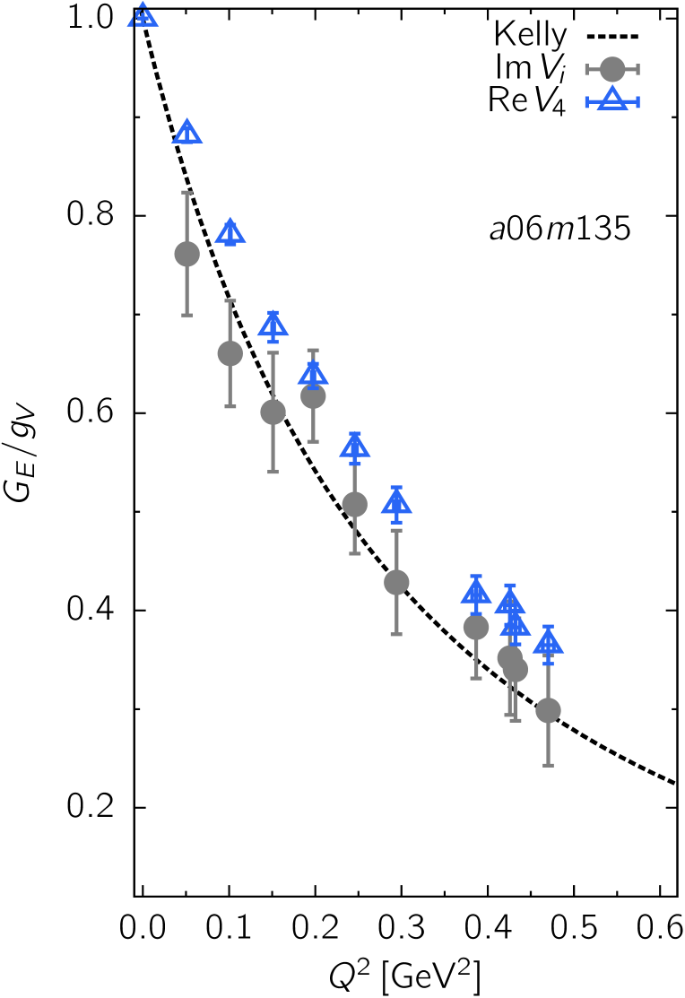
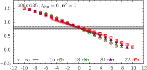
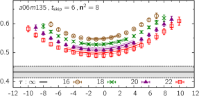
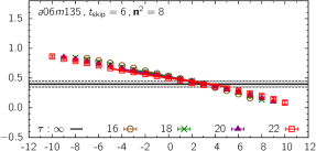
Figure 1: (left) Comparison of $G_{E}(Q^{2})$ from $\;\mathrm{Im}V_{i}$ versus $\;\mathrm{Re}V_{4}$. (middle) Excited state effects in matrix element of $\;\mathrm{Re}V_{4}$ and (right) $\;\mathrm{Im}V_{i}$. All data are from the physical mass ensemble $a06m135$.

The continuum-chiral-finite-volume (CCFV) fits for the electric and magnetic charge radii, $\langle r_{E}^{2}\rangle$ and $\langle r_{M}^{2}\rangle$, and magnetic moment, $\mu$, are carried out including the leading order terms that describe lattice artifacts due to finite lattice spacing $a$, and variation with pion mass $M_{\pi}$ and finite volume parameter $M_{\pi}L$ using expressions taken from Refs. [7, 8, 9].

$$\langle r_{E}^{2}\rangle(a,M_{\pi},L)=c_{1}^{E}+c_{2}^{E}a+c_{3}^{E}\ln(M_{\pi}^{2}/\lambda^{2})+c_{4}^{E}\ln(M_{\pi}^{2}/\lambda^{2})\exp(-M_{\pi}L)\,,$$ (3)

$$\langle r_{M}^{2}\rangle(a,M_{\pi},L)=c_{1}^{M}+c_{2}^{M}a+c_{3}^{M}/M_{\pi}+c_{4}^{M}/M_{\pi}\exp(-M_{\pi}L)\,,$$ (4)

$$\mu(a,M_{\pi},L)=c_{1}^{\mu}+c_{2}^{\mu}a+c_{3}^{\mu}M_{\pi}+c_{4}^{\mu}M_{\pi}\left(1-\frac{2}{M_{\pi}L}\right)\exp(-M_{\pi}L)\,.$$ (5)

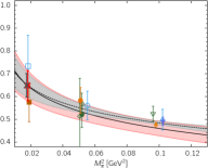
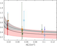
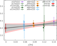
Figure 2: CCFV fits (pink band) plotted versus the variable they are most sensitive to. Fits to $\langle r_{E}^{2}\rangle$ (left) and $\langle r_{M}^{2}\rangle$ (middle), both in $\fm^{2}$, highlight the non-analytical dependence on $M_{\pi}$ given in Eqs. (3) and (4). (right) CCFV fit for magnetic moment $\langle\mu\rangle$ is plotted versus $a$. In contrast, the gray band in each panel is the result of fits versus the single variable defining the x-axis.

We first analyze the $Q^{2}$ dependence of form factors for each of the 14 calculations using the dipole and model independent $z$-expansions. Then recognizing that the two pairs, $a06m220(W)$ and $a06m310(W)$, share the same gauge ensemble but only the smearing widths are different, we construct 11-point data by averaging the $\langle r_{M}^{2}\rangle$, $\langle r_{M}^{2}\rangle$ and $\mu$ values from the two smearings assuming full correlations, and dropping the $a09m130$ data because the bias correction is not available for $Q^{2}\neq 0$. We further construct two 10-point data sets by excluding (i) the coarsest lattice spacing $a15m310$ or (ii) the smallest volume $a12m220S$ data. The CCVF fits for getting the final $\langle r_{E}^{2}\rangle$, $\langle r_{M}^{2}\rangle$, and $\mu$, are then performed for for each of the data sets: 14-point, 11-point, 10-point and $10^{\ast}$-point and for the dipole and various $z$-expansion analysis of $Q^{2}$ behavior. In these fits, the 14, 11, 10 or $10^{\ast}$ data points are treated as uncorrelated.

The variation of $\langle r_{E}^{2}\rangle$ between the 14 calculations and between dipole and $z$-expansion analysis is small as shown in Fig. 3. The figure also shows the results from the 14-, 11-, 10-, and 10^∗-point CCFV fits. We take the central value for $\langle r_{E}^{2}\rangle$ from the 11-point fit with the $z^{3+4}$ truncation of the $z$-expansion. This is given in Table 1. Note that $z^{i+4}$ fits include the four sum rule constraints imposed to ensure that $G_{A,E,M}(Q^{2})\to 0$ as $1/Q^{4}$ for large $Q^{2}$. For $\langle r_{M}^{2}\rangle$ and $\mu$, we take the central values from $z^{3}$ as the $z^{3+4}$ fits are unstable. The reason $G_{M}$ fits are less stable is the point $G_{M}(0)$, which would pin the fit at $Q^{2}=0$ is not calculable from lattice simulations. The CCFV fits for $\langle r_{E}^{2}\rangle$, $\langle r_{M}^{2}\rangle$, and $\langle\mu\rangle$ are shown in Fig. 2 versus the variable they vary the most with.

The magnetic moment $\mu$ from either the dipole or the $z$-expansion analysis is about $15\%$ smaller than the experimental value $\mu^{\text{exp}}=4.7058$ as can be inferred from the data for $\mu^{\text{exp}}G_{E}/G_{M}$ plotted in Fig. 4. Since the ratio $G_{E}/G_{M}$ is insensitive to $a$ or $M_{\pi}$, the low value of $\mu$ obtained is not simply explained by the less stable fits to $G_{M}$ versus $Q^{2}$. Also, the size and quality of the ESC in $\;\mathrm{Re}V_{i}$ (averaged over $i=1,2$ as these two are related by the lattice rotational symmetry) is similar to $\;\mathrm{Re}V_{4}$ shown in Fig. 1, and the 2- and $3^{\ast}$-state fits give stable estimates of the $\tau\to\infty$ value.

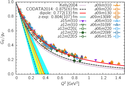
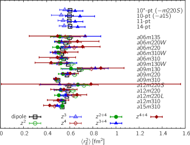
Figure 3: (left) Isovector electric form factor $G_{E}^{u-d}(Q^{2})/g_{V}$ compared to the Kelly parameterization, and dipole fit with CODATA value of $\langle r_{E}\rangle$. The straight lines represent the slope at $Q^{2}=0$ for each fit. The yellow inner band and cyan outer band are the statistical and systematical errors in the $z$-expansion. (right) Values of $\langle r_{E}^{2}\rangle$ from the CCFV fits for the 14 calculations, each with the dipole and $z$-expansion analysis of the $Q^{2}$ behavior.

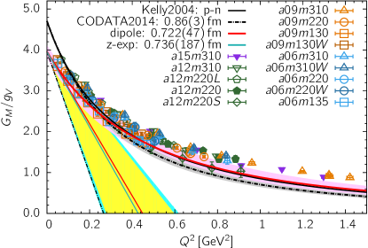
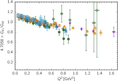
Figure 4: (left) Data for the isovector magnetic form factor $G_{M}^{u-d}(Q^{2})$. To allow a visual comparison of the slope at $Q^{2}=0$, different values of $\mu=G_{M}(0)$ are shifted to a common point taken to be the dipole result. (right) Data for the ratio $\mu^{\text{exp}}G_{E}/G_{M}$ with $\mu^{\text{exp}}=4.7058$.

3 Axial Form Factors

The form factor decomposition of the matrix element of the isovector axial-vector current between nucleon states is:

$$\left\langle N(\bm{p}_{f})|A_{\mu}(\bm{q})|N(\bm{p}_{i})\right\rangle =\;{\overline{u}}_{N}(\bm{p}_{f})\left(G_{A}(Q^{2})\gamma_{\mu}+q_{\mu}\frac{\tilde{G}_{P}(Q^{2})}{2M_{N}}\right)\gamma_{5}u_{N}(\bm{p}_{i})\,.$$ (6)

We follow the same procedure for controlling the ESC in the matrix elements and for the extraction and CCFV fits to the axial charge radius as for the electromagnetic form factors described in Sec. 2. The CCFV fit for $\langle r_{A}^{2}\rangle$ is made using

$$\langle r_{A}^{2}\rangle(a,M_{\pi},L)=c_{1}^{A}+c_{2}^{A}a+c_{3}^{A}M_{\pi}^{2}+c_{4}^{A}M_{\pi}^{2}\exp(-M_{\pi}L)\,,$$ (7)

and results for the $z^{3+4}$ analysis are shown in Fig. 5. All the data versus $Q^{2}$ are shown in Fig. 6 (left), and the variation versus different fit ansatz is shown in Fig. 6 (right). The central values are taken from the 11-point CCFV fit and results for the dipole and $z^{3+4}$ analysis are given in Tab. 1.

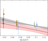
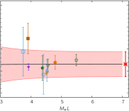
Figure 5: CCFV fits for the axial charge radius $\langle r_{A}^{2}\rangle$ in fm². The three panels show the fits versus the lattice spacing (left) pion mass (middle) and finite box size parameter $M_{\pi}L$ (right), with the other variables in Eq. (7) set to their physical values.

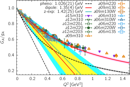
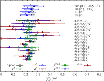
Figure 6: (left) Data for the axial-vector form factor $G_{A}^{u-d}(Q^{2})/g_{A}$. The straight lines show the slope at $Q^{2}=0$ for the dipole and $z$-expansion fits. The dashed-dotted line is the dipole fit with the phenomenological estimate $M_{A}=1.026$. (right) The values of $\langle r_{A}^{2}\rangle$ from the four CCFV fits, and from the 14 calculations with both the dipole and $z$-expansion analysis of the $Q^{2}$ behavior.

4 Discussion and Outlook

Results for the charge radii $\sqrt{\langle r_{E}^{2}\rangle}$, $\sqrt{\langle r_{M}^{2}\rangle}$, $\sqrt{\langle r_{A}^{2}\rangle}$ and magnetic moment $\mu$ from isovector electromagnetic and axial form factors are summarized in Tab. 1. The $z$-expansion results have larger errors in all cases, and the dipole results are consistant with these within statistical errors. Compared to the previous works [3, 5], the errors in the dipole estimates are smaller with increased statistics and ensembles, but only in $r_{E}$ for the $z$-expansion. Part of the reason is that in Refs. [3, 5], the $z$-expansion results were averaged: $z^{2}$ and $z^{3}$ for $\langle r_{M}^{2}\rangle$ and $\mu$, and $z^{2+4}$ and $z^{3+4}$ for $\langle r_{E}^{2}\rangle$ and $\langle r_{A}^{2}\rangle$. As a result, these errors quoted were dominated by the smaller error points $z^{2}$ or $z^{2+4}$, while the new results are taken from the higher order truncation, $z^{3}$ or $z^{3+4}$, that have larger errors. The more pressing challenge with the $z$-expansion analysis is to show stability with respect to the order of the truncation.

We now also quote a systematic error from the CCFV fits. For ${\langle r_{E}^{2}\rangle}$ and ${\langle r_{M}^{2}\rangle}$, the dominant variation is with respect to $M_{\pi}^{2}$, so we take it to be the difference between the two physical pion mass ensemble results. For the magnetic moment, the largest variation is with $a$, so we take the difference between the CCFV fit result and the average of the five finest lattice, $a\approx 0.06\fm$, results. These conservative estimates will be refined in future work.

Adding the statistical and systematic errors in quadrature, our lattice estimates for $r_{E}$ are consistent with the Kelly parameterization of the experimental data for the isovector combination. Clearly, the current precision in the lattice data is not sufficient to address the proton charge radius puzzle. The lattice estimate of the magnetic charge radius $r_{M}$ has an even larger error. The magnetic moment $\mu$ from our calculation undershoots the experimental value by $15\%$, with the $a\approx 0.06\fm$ data pulling down the CCFV fit. The range of parameter values analyzed in this work leaves open the possibility that the finite volume effects are significant, especially at the lowest $Q^{2}$ value [10]. For the future, better control over extrapolation to the physical limit would include a modified CCFV fit that includes higher order corrections from an effective theory such as HB$\chi$PT [9], and by combining this fit with the $Q^{2}$ behavior as discussed in Ref. [11].

The axial charge radius $r_{A}$ is smaller than the value extracted from from neutrino scattering data, $r_{A}=0.666(17)\fm$, from electroproduction, $r_{A}=0.639(10)\fm$, and from a reanalysis of deuterium data, $r_{A}=0.68(16)\fm$. In Ref. [3], we had pointed out a problem with the lattice estimates of the axial $G_{A}$, induced pseudoscalar $\widetilde{G}_{P}$, and pseudoscalar $G_{P}$ form factors: while the PCAC relation is satisfied at the correlator level, it is not satisfied by the form factors. This problem is under investigation.

		$r_{E}\,[\mathrm{fm}]$	$r_{M}\,[\mathrm{fm}]$	$\mu$	$r_{A}\,[\mathrm{fm}]$	$\mathcal{M}_{A}\,[\mathrm{GeV}]$
This work	$z$-exp.	0.804(42)(98)	0.736(166)(86)	3.99(32)(17)	0.481(58)(62)	1.42(17)(18)
	dipole	0.772(10)(8)	0.722(23)(41)	3.96(10)(12)	0.505(13)(6)	1.35(3)(2)
Jang  et. al.[5]	$z$-exp.	0.83(9)	0.82(10)	3.47(36)	0.50(6)	1.36(17)
	dipole	0.79(3)	0.77(4)	3.72(23)	0.51(2)	1.34(6)
Gupta  et.al.[3]	$z$-exp.				0.46(6)	1.48(19)
	dipole				0.49(3)	1.39(9)

Table 1: Summary of charge radii, magnetic moment, and axial mass from isovector form factors. When two errors are given, the first is statistical and the second is systematic.

References

- [1] A. Bazavov et al., MILC, Phys. Rev. D87 (2013), no. 5 054505, [1212.4768].
- [2] T. Bhattacharya, S. D. Cohen, R. Gupta, A. Joseph, H.-W. Lin, and B. Yoon, Phys. Rev. D89 (2014), no. 9 094502, [1306.5435].
- [3] R. Gupta, Y.-C. Jang, H.-W. Lin, B. Yoon, and T. Bhattacharya, Phys. Rev. D96 (2017), no. 11 114503, [1705.06834].
- [4] R. Gupta, Y.-C. Jang, B. Yoon, H.-W. Lin, V. Cirigliano, and T. Bhattacharya, Phys. Rev. D98 (2018) 034503, [1806.09006].
- [5] Y.-C. Jang, T. Bhattacharya, R. Gupta, H.-W. Lin, and B. Yoon, EPJ Web Conf. 175 (2018) 06033, [1801.01635].
- [6] P. J. Mohr, D. B. Newell, and B. N. Taylor, Rev. Mod. Phys. 88 (2016), no. 3 035009, [1507.07956].
- [7] S. R. Beane, Phys. Rev. D70 (2004) 034507, [hep-lat/0403015].
- [8] M. Gockeler, T. R. Hemmert, R. Horsley, D. Pleiter, P. E. L. Rakow, A. Schafer, and G. Schierholz, QCDSF, Phys. Rev. D71 (2005) 034508, [hep-lat/0303019].
- [9] V. Bernard, H. W. Fearing, T. R. Hemmert, and U. G. Meissner, Nucl. Phys. A635 (1998) 121–145, [hep-ph/9801297]. [Erratum: Nucl. Phys.A642,563(1998)].
- [10] B. C. Tiburzi, Phys. Rev. D77 (2008) 014510, [0710.3577].
- [11] G. S. Bali, S. Collins, M. Gruber, A. Schäfer, P. Wein, and T. Wurm, 1810.05569.