Determining Principal Component Cardinality
through the
Principle of Minimum Description Length

Abstract

PCA (Principal Component Analysis) and its variants are ubiquitous techniques for matrix dimension reduction and reduced-dimension latent-factor extraction. One significant challenge in using PCA, is the choice of the number of principal components. The information-theoretic MDL (Minimum Description Length) principle gives objective compression-based criteria for model selection, but it is difficult to analytically apply its modern definition - NML (Normalized Maximum Likelihood) - to the problem of PCA. This work shows a general reduction of NML problems to lower-dimension problems. Applying this reduction, it bounds the NML of PCA, by terms of the NML of linear regression, which are known.

1 Introduction

1.1 The Problem of Principle Component Dimension Selection

Let $X$ be an an $n\times m$ matrix. In machine learning, it is very common to approximate it by a “simpler” product of matrices $W$ and $Z^{T}$ of lower dimensions $n\times k$ and $k\times m$, respectively (for $k\lneq m$). Among others, these include Probabilistic Principal Component Analysis, Independent-Factor Analysis, and Non-Negative Matrix Factorization (see [12, 26, 3]). We will focus specifically on the simple PCA (Principal Component Analysis),

$$\arg\min_{W,Z:\;\mathop{\mathrm{rank}}\left(W\right)=\mathop{\mathrm{rank}}\left(Z\right)=k}\left\lVert X-WZ^{T}\right\rVert_{F}^{2}.$$ (1)

The lower-dimension product is not guaranteed to losslessly approximate the original matrix. In fact, the famous Eckart-Young-Mirsky Theorem - whose properties we will use throughout - essentially guarantees some loss:

Theorem 1.1

(Eckart-Young-Mirsky) Let $X=U\Lambda V^{T}$ be the SVD (singular value decomposition) of $X$, with $\Lambda=\mathop{\mathrm{diag}}\left(\lambda_{1},\ldots,\lambda_{m}\right)$, and $U$ and $V$ unitary. Let $U_{k}$ and $V_{k}$ be the matrices of the first $k$ columns of $U$ and $V$, respectively. Then

$$\begin{split}&\left\lVert X-WZ^{T}\right\rVert_{F}^{2}\geq\left\lVert X-U_{k}\mathop{\mathrm{diag}}\left(\lambda_{1},\ldots,\lambda_{k}\right)V_{k}\right\rVert_{F}^{2}=\sum_{i=k+1}^{m}\left[\lambda_{i}^{2}\right],\end{split}$$ (2)

and so $W=U_{k}\mathop{\mathrm{diag}}\left(\lambda_{1},\ldots\lambda_{k}\right)$, $Z=V_{k}$, is optimal.

The motivation for the reduced dimension, is uncovering a structure that is, in some sense, “truer”, or “more useful”. To quote [15]:

The central idea of principal component analysis is to reduce the dimensionality of a data set in which there are a large number of interrelated variables, while retaining as much as possible of the variation present in the data set. This reduction is achieved by transforming to a new set of variables, the principal components, which are uncorrelated, and which are ordered so that the first few retain most of the variation present in all of the original variables.

As the theorem shows, though, loss minimization, in itself, will not lead us to the reduced dimension - it will always favor the maximum number of components.

1.2 The Principles of MDL and NML

The MDL (minimum description length) principle (see [10, 18, 9, 23, 21]) is an information-theoretic method for model selection. Probability-theory approaches to model selection - both frequentist and Bayesian - assume that there exists a true probability distribution from which the observed data were sampled. The goal is to optimize a model subject to this (indirectly-observed) distribution. MDL is similar in philosophy to Occam’s Razor (see [2]). The goal is to find a model optimizing the total description length of the model and the observed data. There is no assumption that a true probability was approximated, or that it even exists. We will see that avoiding this assumption leads to a form of online optimality.

How can we objectively quantify a description length? Given a probability distribution, information theory gives an objective code length through entropy [6], but assumptions on the probability distribution are precisely what we wish to avoid. In [24], Rissanen formulated the question as a minimax problem, namely the smallest regret relative to all possible codes under mild conditions. He showed that the NML (Normalized Maximum Likelihood) (see [24, 1]) is the solution to this problem.

Definition 1

Normalized Maximum Likelihood Let $X$ be distributed by a model specified by some parameter(s) $\Phi$. The NML is defined as

$$f^{\mathrm{NML}}\left(X\right)={\hat{f}\left(X\;;\;\hat{\Phi}\left(X\right)\right)\over\int\limits{\hat{f}\left(Y\;;\;\hat{\Phi}\left(Y\right)\right)}\,\textrm{d}{Y}},$$ (3)

where

• $\hat{\Phi}\left(X\right)$ is the maximum likelihood (ML) estimator of $\Phi$ given $X$.

• $\hat{f}\left(Y\;;\;\hat{\Phi}\left(Y\right)\right)$ is the ML of $Y$ assuming that the true parameters are $\hat{\Phi}\left(Y\right)$.

The logarithm of the right-hand side of Equation (3) is the stochastic complexity, and the logarithm of its denominator is the parametric complexity. It can be shown that choosing between different $\Phi$ based on maximizing (3), is optimal in a prequential sense (see [20]).

1.3 Main Contribution: Applying NML to PCA

Conceptually, it is possible to calculate the NML of PCA, by inserting equation (2) into equation (3). Unfortunately, evaluating the denominator requires integrating over the eigenvalues of arbitrary matrices, which is difficult. Instead, in the rest of this paper, we avoid this by bounding the NML of PCA by reducing it to the NML of linear regression (see [22]), resulting in the following theorem:

Theorem 1.2

Let $s\left(X\;;\;k\right)$ be the stochastic complexity of a $k$-dimensional PCA reduction of $X$. Then

$$\begin{split}&s(X\;;\;k)\\ &\;\;\simeq\left(nm-kn\right)\mathop{\mathrm{ln}}\left(\sum_{i=k+1}\left[\lambda_{i}^{2}\right]\right)+nk\mathop{\mathrm{ln}}\left(\left\lVert X^{T}X\right\rVert_{F}^{2}\right)\\ &\;\;+(mn-kn-1)\mathop{\mathrm{ln}}\left(mn\over mn-kn\right)-(nk+1)\mathop{\mathrm{ln}}\left(nk\right)+\Delta s,\end{split}$$ (4)

where

$$\begin{split}0&\leq\Delta s\leq mk\mathop{\mathrm{ln}}\left(2\over m\epsilon\right).\end{split}$$ (5)

This means that the number of dimensions can be chosen, by optimizing the above for $k$.

1.4 Outline

We continue this section with definitions and notations, and related work. Section 2 shows the main idea of NML reduction via elimination of some of the optimization parameters. We use this to reduce the problem of PCA NML to linear-regression NML. Section 3 details the specific reductions. Section 4 shows numerical experiments. Section 5 concludes and discusses further work.

1.5 Definitions and Notations

We will use lowercase letters ($s$) for scalars, underlined lowercase letters ($\underline{x}$) for column vectors, uppercase letters ($X$) for matrices, and calligraphic ($\mathcal{B}$) for sets. A single subscript for a matrix denotes a matrix row ($X_{i}$). $f\left(x\right)$, $f\left(x\;;\;y\right)$, $f\left(x\;|\;y\right)$ denote the density of some $x$, the density of some $x$ assuming some other parameter is $y$, and the density of some $x$ conditional on some other random variable being $y$, respectively. $\left\lVert X\right\rVert_{F}=\left(\sum_{i,j}X_{i,j}^{2}\right)^{1\over 2}$ is the Forbenius norm, and $D\left({x}\;|\;{y}\right)$ is the Kullback-Leibler distance.

1.6 Related Work

[3, 26] contain excellent overviews of matrix factorization; in particular, PCA appears in the classic [8]. [18, 11, 24, 9, 10, 1] describe MDL and NML, in particular, for model selection. [22, 24] show closed forms of linear-regression NML. [16] uses cross validation approximations for PCA dimension estimation, [5] does so using an analysis of the conditional distribution of the singular values of a Wishart matrix, [13] uses a Bayesian approach, [29] uses patterns in the scree plots, and [14] compares statistical and heuristic approaches to this problem. To the best of my knowledge, previous works did not apply the modern form of the MDL principle to the problem of PCA dimension selection.

2 NML reduction via Elimination of Optimization Parameters

Consider the generative form of (1), shown in the factor diagram (see [7]) in Figure 1. In this model, $k\sim\mathcal{U}(1,m)$ determines the dimension of $W_{k}$ and $V_{k}$. $X=W_{k}V_{k}^{T}+\Upsilon$, where $\Upsilon\sim\mathcal{N}\left(0,\tau I_{k}\right)$. Note that they do not appear in the original problem (at least in this form), but the problems are effectively equivalent. The distribution of $k$ hardly affects the stochastic complexity (see [21], Chapter 5), and any distribution assigning a positive probability to any value of $1,\ldots,m$ could be used. Regarding the Gaussian additive noise $\Upsilon$,

$$\begin{split}&\arg\max_{W_{k},V_{k}}f\left(X\;;\;k\right)=\arg\max_{W_{k},V_{k}}{1\over\left(2\pi\tau\right)^{{nm\over 2}}}e^{-{\left\lVert X-W_{k}V_{k}^{T}\right\rVert_{F}^{2}\over 2\tau^{2}}}\mathrel{\overset{\makebox[0.0pt]{\mbox{\tiny(a)}}}{=}}\sum_{i=k+1}^{m}\left[\lambda_{i}^{2}\right],\end{split}$$

where (a) follows from Theorem 1.1.

Now consider the generative model in Figure 4 (discussed in greater detail in Section 3), where both the number of parameters and the loadings matrix are known. This easier problem is more similar to linear regression, whose NML is known (see [22]). Of course, in the original problem, the loadings matrix is not known, but rather optimized as well. The following Lemma, however, relates the NML of a problem depending on a number of parameters, to the the same problem where one of them is fixed.

Figure 1: Equivalent factor graph of PCA. The dimension $k$ is a-priori uniform, and the observed matrix $X$ is the product of the score and loadings matrices, with additive noise $\Upsilon$ distributed i.i.d. $\mathcal{N}\left(0,\tau I_{k}\right)$.

Lemma 1

Let $\mathcal{B}=\left\{b_{1},\ldots,b_{\ell}\right\}$ be a finite set (for some $\ell$). Then

$$\begin{split}&\int\limits{\hat{f}\left(X\;|\;\hat{A}\left(X\right),\hat{b}\left(X\right)\right)}\,\textrm{d}{X}\leq\sum_{b\in\mathcal{B}}\int\limits{\hat{f}\left(X\;|\;\hat{A}\left(X\right),b\right)}\,\textrm{d}{X}.\end{split}$$ (6)

Furthermore, if

$$\hat{b}\left(x\right)=\arg\min_{b}\hat{f}\left(X\;|\;\hat{A}\left(X\right),b\right),$$ (7)

then

$$\begin{split}&\int\limits{\hat{f}\left(X\;|\;\hat{A}\left(X\right),\hat{b}\left(X\right)\right)}\,\textrm{d}{X}\geq\max_{b\in\mathcal{B}}\int\limits{\hat{f}\left(X\;|\;\hat{A}\left(X\right),b\right)}\,\textrm{d}{X}.\end{split}$$ (8)

Figure 2: Parametric complexity using only a subset of the features. For each $X$, there are an optimal $\hat{A}\left(X\right)$ and $\hat{b}\left(x\right)$, but we wish to bound this by expressions in which for each $X$, $b$ is constant.

Proof

For inequality (6),

$$\begin{split}&\int\limits_{X}{\hat{f}\left(X\;|\;\hat{A}\left(X\right),\hat{b}\left(X\right)\right)}\,\textrm{d}{X}=\sum_{b}\int\limits_{X:\;\hat{b}\left(X\right)=b}{\hat{f}\left(X\;|\;\hat{A}\left(X\right),b\right)}\,\textrm{d}{X}\\ &\;\;\mathrel{\overset{\makebox[0.0pt]{\mbox{\tiny(a)}}}{\leq}}\sum_{b}\int\limits_{X}{\hat{f}\left(X\;|\;\hat{A}\left(X\right),b\right)}\,\textrm{d}{X},\end{split}$$

where (a) follows from the non-negativity of densities. In Figure 2, this corresponds to bounding by considering the sum of all planes, then slicing them by vertical levels.

For inequality (8), consider an arbitrary $b^{\prime}\in\mathcal{B}$. Then

$$\begin{split}&\int\limits_{X}{\hat{f}\left(X\;|\;\hat{A}\left(X\right),\hat{b}\left(X\right)\right)}\,\textrm{d}{X}=\sum_{b}\int\limits_{X:\;\hat{b}\left(X\right)=b}{\hat{f}\left(X\;|\;\hat{A}\left(X\right),b\right)}\,\textrm{d}{X}\\ &\;\;=\int\limits_{X:\;\hat{b}\left(X\right)=b^{\prime}}{\hat{f}\left(X\;|\;\hat{A}\left(X\right),b^{\prime}\right)}\,\textrm{d}{X}+\sum_{b\neq b^{\prime}}\int\limits_{X:\;\hat{b}\left(X\right)=b}{\hat{f}\left(X\;|\;\hat{A}\left(X\right),b\right)}\,\textrm{d}{X}\\ &\;\;\mathrel{\overset{\makebox[0.0pt]{\mbox{\tiny(a)}}}{\geq}}\int\limits_{X:\;\hat{b}\left(X\right)=b^{\prime}}{\hat{f}\left(X\;|\;\hat{A}\left(X\right),b^{\prime}\right)}\,\textrm{d}{X}+\sum_{b\neq b^{\prime}}\int\limits_{\hat{b}\left(X\right)=b}{\hat{f}\left(X\;|\;\hat{A}\left(X\right),b^{\prime}\right)}\,\textrm{d}{X}\\ &\;\;=\int\limits_{X}{\hat{f}\left(X\;|\;\hat{A}\left(X\right),b^{\prime}\right)}\,\textrm{d}{X},\end{split}$$

where (a) follows from condition (7). Since this is true for an arbitrary $b^{\prime}$, it is true for the maximum. In Figure 2, this corresponds to moving the disks until they are at the same horizontal level.

The next section formalizes the application of the lemma to PCA NML.

3 Reducing PCA NML to Linear Regression NML

Let $v_{i,j}$ be the elements of the unitary matrix $V$ from Theorem 1.1. By the Cauchy-Schwartz Inequality, $\left\lvert v_{i,j}\right\rvert\leq 1$. Let $\epsilon\lneq{1\over m}$ be a number such that $1\over\epsilon$ is an integer. We can quantize $v_{i,j}$ into one of ${2\over\epsilon}+1$ values, each distanced $\epsilon$ from each other, resulting in the matrix $V^{\epsilon}$. By considering its Neumann series, it is clear that it is invertible, so there exists some $W^{\prime}$ such that $W^{\prime}V^{\epsilon}=WV$.

Using Lemma 1, therefore, we can reduce the original problem to that in Figure 3, where $V_{k}^{\epsilon}$ is a known matrix which is quantized version of a unitary matrix $V_{k}$ (specifically, $V_{k}^{\epsilon}=V_{k}+\epsilon E_{k}$, where $E_{k}$ has values each with absolute value at most $1\over 2$). Let $\mathcal{V}_{k}^{\epsilon}$ be the set of the quantized matrices, and let $s_{i}^{\epsilon}(X,k)$ be the stochastic complexity of Figure 3, where the loadings matrix is known to be the $i$th element of $\mathcal{V}_{k}^{\epsilon}$ (according to some enumeration). Then by Lemma 1,

$$\max_{i\in\left\{1,\ldots,\left\lvert\mathcal{V}_{k}^{\epsilon}\right\rvert\right\}}s_{i}^{\epsilon}\left(X\;;\;k\right)\leq s\left(X\;;\;k\right)\leq\sum_{i=1}^{\left\lvert\mathcal{V}_{k}^{\epsilon}\right\rvert}\left[s_{i}^{\epsilon}\left(X\;;\;k\right)\right].$$ (9)

Furthermore, we will see in Appendix 0.A.1 the following lemma:

Lemma 2

$$\begin{split}\mathop{\mathrm{ln}}\left(\left|\mathcal{V_{k}^{\epsilon}}\right|\right)\lesssim mk\mathop{\mathrm{ln}}\left(\left({2\over\epsilon}+1\right)e^{-\left({1-{1+\epsilon+{\epsilon^{2}\over 4}\over\sqrt{m}}\over 2}\right)}\right)+(k-1)\mathop{\mathrm{ln}}\left(\epsilon+{m\epsilon^{2}\over 4}\over\pi\right).\end{split}$$ (10)

Figure 3: Factor graph of known quantized loadings ”PCA”.

Let $V_{k}^{\epsilon}$, a known quantized loadings matrix, be the $i$th item in $\mathcal{V_{k}^{\epsilon}}$. To calculate its NML, note that Figure 3 is very similar to linear regression (whose NML is known), except that $W_{k}$ and $X$ are matrices instead of vectors. This can be easily reduced to linear regression, though, by considering the problem

$$\begin{split}&\underline{x}=\tilde{V_{k}}^{\epsilon}\underline{w}+\underline{\upsilon}\\ &\;\;=\begin{bmatrix}X_{1}^{T}\\ \vdots\\ X_{n}^{T}\end{bmatrix}=\begin{bmatrix}V_{k}^{\epsilon}&\ldots&0\\ \vdots&\ddots&\vdots\\ 0&\ldots&V_{k}^{\epsilon}\end{bmatrix}\begin{bmatrix}W_{1}^{T}\\ \vdots\\ W_{n}^{T}\end{bmatrix}+\begin{bmatrix}\Upsilon_{1}^{T}\\ \vdots\\ \Upsilon_{n}^{T}\end{bmatrix},\end{split}$$

where $\underline{x}$ and $\underline{\upsilon}$ each have length $nm$, $\tilde{V_{k}}^{\epsilon}$ is $mn\times kn$, and $\underline{w}$ has length $km$. This is the dashed part of Figure 4, and has known NML (see Equation (19) in [22])

$$\begin{split}&s_{i}^{\epsilon}(X,k)=\left(nm-kn\right)\mathop{\mathrm{ln}}\left(\hat{\tau}\right)+nk\mathop{\mathrm{ln}}\left(\left\lVert\tilde{V}_{k}^{\epsilon}\hat{w}\right\rVert_{F}^{2}\right)\\ &\;\;+(mn-kn-1)\mathop{\mathrm{ln}}\left(mn\over mn-kn\right)-(nk+1)\mathop{\mathrm{ln}}\left(nk\right).\end{split}$$ (11)

However, we need the NML to be expressed in terms from the original problem.

Figure 4: Linear-regression factor graph.

It is well known (see [12]) that

$$\begin{split}&\underline{\hat{w}}=\begin{bmatrix}\left(V_{k}^{\epsilon T}V_{k}^{\epsilon}\right)^{-1}V_{k}^{\epsilon T}X_{1}^{T}\\ \vdots\\ \left(V_{k}^{\epsilon T}V_{k}^{\epsilon}\right)^{-1}V_{k}^{\epsilon T}X_{n}^{T}\end{bmatrix}.\end{split}$$

Furthermore, for the $j$th range,

$$\begin{split}&\hat{W}_{j}^{T}=\left(V_{k}^{\epsilon T}V_{k}^{\epsilon}\right)^{-1}V_{k}^{\epsilon T}X_{j}^{T}\\ &\;\;\simeq\left(I_{k}+\epsilon\left(V_{k}^{T}E+E^{T}V_{k}\right)\right)^{-1}V_{k}^{T}X_{j}^{T}\\ &\;\;\mathrel{\overset{\makebox[0.0pt]{\mbox{\tiny(a)}}}{\simeq}}\left(I_{k}-\epsilon\left(V_{k}^{T}E+E^{T}V_{k}\right)\right)V_{k}^{T}X_{j}^{T},\end{split}$$

where (a) follows from [19] Equation (191). Therefore,

$$\begin{split}\left(V_{k}+\epsilon E\right)\hat{W}_{j}^{T}\simeq\left(I_{k}-\epsilon\left({V_{k}^{T}E+E^{T}V_{k}}+EV_{k}^{T}\right)\right)X_{j}^{T},\end{split}$$

and, finally,

$$\begin{split}\left\lvert\mathop{\mathrm{ln}}\left(\left\lVert V_{k}^{\epsilon}\hat{W}_{j}^{T}\right\rVert_{F}^{2}\right)-\mathop{\mathrm{ln}}\left(X_{j}^{T}X_{j}\right)\right\rvert\lesssim 2\epsilon.\end{split}$$ (12)

We now prove Theorem 1.2:

Proof

In equation (11), we replace $\hat{\tau}$ using Theorem 2, and $\tilde{V}_{k}^{\epsilon}\hat{w}$ using equation (12). We use the resulting expression - which is independent from $i$ (the element of $\mathcal{V}_{k}^{\epsilon}$) - in Lemma 1.

4 Numerical Experiments

For numerical experiments we use the Dow-Jones Industrial Index (DJIA), with up to 2030 days, and 30 closing prices. We transform the $i,j$-th entry, $c_{i,j}$ denoting the closing price of stock $j$ at day $i$, to $100{c_{i,j}-c_{i-1,j}\over c_{i-1,j}}$, i.e., the relative closing price in percentage (see [28]). In the following, Orig is this matrix; Lin10 is a matrix whose first 10 columns are the original ones, and the last 20 are a random linear combination of the first 10, with $\mathcal{N}\left(0,0.1\right)$ noise added; Lin5 is the same, but with the last 25 generated from the first 5. By the construction, it is apparent that, at least for large enough datasets, the correct number of principal components should be 30, 10, and 5, respectively.

Consider the variance explained by the principle components for the three datasets. This is typically done via a scree plot (see [4, 29]), which Figure 5 shows for these datasets. The horizontal axis in the plot shows the indexing of the principal components ordered by the magnitudes of eigenvalues. The vertical axis shows the variance explained by each of the components. As is typical for scree plots, the first few principal components explain much more of the variance than latter ones. In fact, there seems to be a “bend” in the plot for each one of the datasets, that can indicate the optimal number of components. Unfortunately, the plots for the three datasets seem to be very similar, and their “bends” seem to be at around the same number of components. It is not apparent to judge, by eye, what number of components should be used.

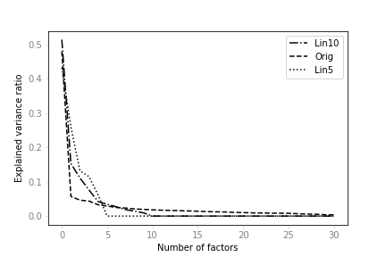
Figure 5: Scree plots for the three datasets.

Using the Kneedle algorithm (see [25]) for finding “bends” in plots, we get the estimated optimal number of components, as a function of the dataset length, in Figure 6. This method is known for its tendency to find a lower number of components than the true one (see [27]), as is indeed the case here.

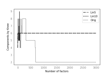
Figure 6: Optimal components using the knee method.

The Kaiser method (see [15]) takes components whose eigenvalues are at least one. Figure 7 shows the estimated optimal number of components, as a function of the dataset length, using this method. While this method does better, it also underestimates the number of components. It is also interesting to note that the results are not monotone in the length of the datasets.

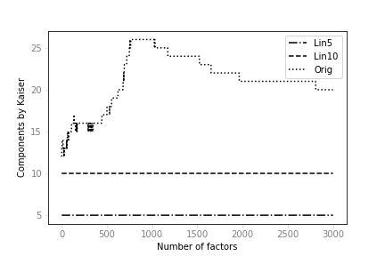
Figure 7: Optimal components using the Kaiser method.

Finally, Figure 8 shows the upper and lower bounds for the optimal number of components as a function of dataset length, using the NML technique from this paper. Note that we don’t have an analytical expression for the NML of PCA, but rather bounds for it. Figure 9 shows the ratio of the bounds as a function of the dataset length.

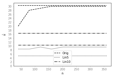
Figure 8: Lower and upper bounds for the optimal $\hat{k}$, for the three datasets.

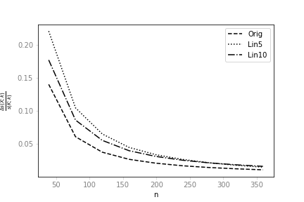
Figure 9: Relative change between the upper and lower bounds of the NML, compared to the NML, for the three datasets.

5 Conclusions and Future Work

In this work we saw an NML-calculation technique based on reducing a problem through eliminating the optimization of some of its original dimensions. We saw how to use this to bound the NML of PCA. The technique is simple and general, and can be used to reduce problems in other domains, where simpler versions of the problem have a closed-form NML. Unfortunately, there are also several types of simple problems with no closed-form NML. For these cases, an MCMC evaluation of the parametric complexity (the denominator of Equation (3)), could be a good numeric approximation. Developing an efficient algorithm for this, is a topic for further research.

Appendix 0.A Appendix

0.A.1 Number of Quantized Unitary Matrices

We prove here Lemma 2. Let $\underline{v_{i}},\underline{v_{j}}$ be two columns of a unitary matrix (perhaps the one), and $\underline{v_{i}^{\epsilon}},\underline{v_{j}^{\epsilon}}$ be their quantized counterparts. Simple arithmetic shows that

$$\left|\underline{v_{i}^{\epsilon}}\cdot\underline{v_{j}^{\epsilon}}-\underline{v_{i}}\cdot\underline{v_{j}}\right|\leq\epsilon+{m\epsilon^{2}\over 4}.$$ (13)

We will see that

$$\begin{split}&P\left(\left|\underline{v_{i}^{\epsilon}}\cdot\underline{v_{i}^{\epsilon}}\right|\leq 1+\epsilon+{\epsilon^{2}\over 4}\right)\leq e^{-mk{1-{{1+\epsilon+{\epsilon^{2}\over 4}}\over\sqrt{m}}\over 2}},\\ &P\left(\left|\underline{v_{i+1}^{\epsilon}}\cdot\underline{v_{i}^{\epsilon}}\right|\leq\epsilon+{\epsilon^{2}\over 4}|\;\forall_{j}\underline{v_{j}}\underline{v_{j}^{\epsilon}}\leq 1+\epsilon+{\epsilon^{2}\over 4}\right)\leq\left({\epsilon+{m\epsilon^{2}\over 4}}\over\pi\right)^{k-1}.\end{split}$$ (14)

For the first part of inequality (14),

$$\begin{split}&P\left(\sum_{k=1}^{m}\left[v_{i,k}^{2}\right]\leq 1+\epsilon+{m\epsilon^{2}\over 4}\right)\leq P\left(\left\lvert\left\{k\;|\;v_{i,k}^{2}\geq x\right\}\right\rvert\leq{1+\epsilon+{m\epsilon^{2}\over 4}\over x}\right)\\ &\;\;\mathrel{\overset{\makebox[0.0pt]{\mbox{\tiny(a)}}}{\leq}}e^{-mD\left({1\over mx}\;|\;{\sqrt{1-x}}\right)},\end{split}$$ (15)

where (a) follow from the Chernoff bound (see [17], Chapter 5). Using the well-known bound (see [6], [17], Chapter 5),

$$D\left({x}\;|\;{y}\right)\geq{(x-y)^{2}\over 2y},\;(x\leq y),$$

and so

$$\begin{split}&D\left({1+\epsilon+{m\epsilon^{2}\over 4}\over mx}\;|\;{\sqrt{1-x}}\right)\geq{\left({1+\epsilon+{m\epsilon^{2}\over 4}\over mx}-\sqrt{1-x}\right)^{2}\over 2\sqrt{1-x}}.\end{split}$$ (16)

Setting $x={1\over\sqrt{m}}$, we have

$$\begin{split}&D\left({1+\epsilon+{m\epsilon^{2}\over 4}\over\sqrt{m}}\;|\;{\sqrt{1-{1\over\sqrt{m}}}}\right)\geq{\left({1+\epsilon+{m\epsilon^{2}\over 4}\over\sqrt{m}}-\sqrt{1-{1\over\sqrt{m}}}\right)^{2}\over 2\sqrt{1-{1\over\sqrt{m}}}}\\ &\;\;\mathrel{\overset{\makebox[0.0pt]{\mbox{\tiny(a)}}}{\simeq}}{\left(1-{3+\epsilon+{\epsilon^{2}\over 4}\over 2\sqrt{m}}\right)^{2}\over 2\left(1-{2\over\sqrt{m}}\right)}\mathrel{\overset{\makebox[0.0pt]{\mbox{\tiny(b)}}}{\simeq}}{1-{1+\epsilon+{\epsilon^{2}\over 4}\over\sqrt{m}}\over 2},\end{split}$$ (17)

where (a) and (b) follow from the Taylor expansion of $(1+x)^{\alpha}$.

For the second part of Inequality (14), applying equation (13) twice on the left side, and once on the right side, we have

$$\underline{v_{i}^{\epsilon}}\cdot\underline{v_{j}^{\epsilon}}=\left\lVert\underline{v_{i}^{\epsilon}}\right\rVert\left\lVert\underline{v_{j}^{\epsilon}}\right\rVert\mathrm{cos}\left(\alpha_{i,k}^{\epsilon}\right),$$ (18)

and so

$${\pi\over 2}-\alpha_{i,k}^{\epsilon}\mathrel{\overset{\makebox[0.0pt]{\mbox{\tiny(a)}}}{\simeq}}\mathrm{sin}\left({\pi\over 2}-\alpha_{i,k}^{\epsilon}\right)=\mathrm{cos}\left(\alpha_{i,k}^{\epsilon}\right)\leq\left\lvert{\epsilon+{m\epsilon^{2}\over 4}\over 1-\epsilon-{m\epsilon^{2}\over 4}}\right\rvert,$$ (19)

with $\alpha_{i,k}^{\epsilon}$ the angle between the vectors, and where (a) follows from the Taylor series of $\mathrm{sin}\left(x\right)$. Approximating $\alpha_{i,k}^{\epsilon}\sim\mathcal{U}\left(0,2\pi\right)$, we get that the probability is approximately that in the second part of Inequality (14).

References

- [1] Andrew R Barron, Jorma Rissanen, and Bin Yu. The Minimum Description Length Principle in Coding and Modeling. IEEE Trans. Inf. Theory, 44(6):2743–2760, 1998.
- [2] Alselm Blumer, Andrzej Ehrenfeucht, David Haussler, and Manfred K. Warmuth. Occam’s razor. Inf. Process. Lett., 24(6):377–380, April 1987.
- [3] Dheeraj Bokde, Sheetal Girase, and Debajyoti Mukhopadhyay. Matrix factorization model in collaborative filtering algorithms: A survey. Procedia Computer Science, 49:136 – 146, 2015. Proceedings of 4th International Conference on Advances in Computing, Communication and Control (ICAC3’15).
- [4] R. B. Cattell. The scree test for the number of factors. Multivariate Behavioral Research, 1:245–276, 1966.
- [5] Yunjin Choi, Jonathan Taylor, and Robert Tibshirani. Selecting the number of principal components: Estimation of the true rank of a noisy matrix. Ann. Statist., 45(6):2590–2617, 12 2017.
- [6] T.M. Cover and J.A. Thomas. Elements of Information Theory. John Wiley and Sons, 2006.
- [7] Laura Dietz. Directed Factor Graph Notation for Generative Models. Technical report, Saarbrücken, Germany, 2010.
- [8] Carl Eckart and Gale Young. The approximation of one matrix by another of lower rank. Psychometrika, 1(3):211–218, Sep 1936.
- [9] Peter Grünwald. A tutorial introduction to the minimum description length principle. In Advances in Minimum Description Length: Theory and Applications. MIT Press, 2005.
- [10] Mark H Hansen and Bin Yu. Model selection and the principle of minimum description length. Journal of the American Statistical Association, 96(454):746–774, 2001.
- [11] Mark H. Hansen and Bin Yu. Minimum description length model selection criteria for generalized linear models, volume Volume 40 of Lecture Notes–Monograph Series, pages 145–163. Institute of Mathematical Statistics, Beachwood, OH, 2003.
- [12] Trevor Hastie, Robert Tibshirani, and Jerome Friedman. The Elements of Statistical Learning. Springer Series in Statistics. Springer New York Inc., New York, NY, USA, 2001.
- [13] David C. Hoyle. Automatic pca dimension selection for high dimensional data and small sample sizes. JMLR, (9):733–2759, 12 2008.
- [14] A. Jackson, Donald. Stopping rules in principal components analysis: A comparison of heuristical and statistical approaches. Ecology, 6(74):2204–2214, 1993.
- [15] I.T. Jolliffe. Principal Component Analysis. Springer Verlag, 1986.
- [16] Julie Josse and François Husson. Selecting the number of components in principal component analysis using cross-validation approximations. Comput. Stat. Data Anal., 56(6):1869–1879, June 2012.
- [17] Michael Mitzenmacher and Eli Upfal. Probability and Computing: Randomized Algorithms and Probabilistic Analysis. Cambridge University Press, Cambridge, 2005.
- [18] J. I. Myung, D. J. Navarro, and M. A. Pitt. Model selection by normalized maximum likelihood. Journal of Mathematical Psychology, 50(2):175–191, 2006.
- [19] K. B. Petersen and M. S. Pedersen. The matrix cookbook, nov 2012. Version 20121115.
- [20] A. Philip Dawid and Vladimir G. Vovk. Prequential probability: principles and properties. Bernoulli, 5(1):125–162, 02 1999.
- [21] J. Rissanen. Stochastic Complexity in Statistical Inquiry. Advanced Series in Applied Physics. World Scientific, 1989.
- [22] Jorma Rissanen. Mdl denoising. IEEE Transactions on Information Theory, 46:2537–2543, 1999.
- [23] Jorma Rissanen. Stochastic complexity. Journal of the Royal Statistical Society, 49(3):223–265, 1999.
- [24] Jorma Rissanen. Strong optimality of the normalized ml models as universal codes. IEEE Transactions on Information Theory, 47:1712–1717, 2000.
- [25] Ville Satopaa, Jeannie R. Albrecht, David E. Irwin, and Barath Raghavan. Finding a ”kneedle” in a haystack: Detecting knee points in system behavior. In 31st IEEE International Conference on Distributed Computing Systems Workshops (ICDCS 2011 Workshops), 20-24 June 2011, Minneapolis, Minnesota, USA, pages 166–171, 2011.
- [26] Madeleine Udell, Corinne Horn, Reza Zadeh, and Stephen Boyd. Generalized low rank models. Foundations and Trends® in Machine Learning, 9(1):1–118, 2016.
- [27] George Lewith Wayne Jonas Harald Walach. Clinical Research in Complementary Therapies 2nd Edition Principles, Problems and Solutions. CRC Press, Churchill Livingstone, 2010.
- [28] Jeffrey M. Wooldridge. Econometric Analysis of Cross Section and Panel Data, volume 1 of MIT Press Books. The MIT Press, 2001.
- [29] Mu Zhu and Ali Ghodsi. Automatic dimensionality selection from the scree plot via the use of profile likelihood. Computational Statistics and Data Analysis, 51:918–930, 2006.