Physics of Arbitrary Doped Kondo Lattices: from
a Commensurate Insulator to a Heavy Luttinger Liquid and a Protected Helical Metal

Abstract

We study one-dimensional Kondo Lattices (KL) which consist of itinerant electrons interacting with Kondo impurities (KI) - localized quantum magnetic moments. We focus on KL with isotropic exchange interaction between electrons and KI and with a high KI density. The latter determines the principal róle of the indirect interaction between KI for the low energy physics. Namely, the Kondo physics becomes suppressed and all properties are governed by spin ordering. We present a first-ever comprehensive analytical theory of such KL at an arbitrary doping and predict a variety of regimes with different electronic phases. They range from commensurate insulators (at filling factors 1/2, 1/4 and 3/4) to metals with strongly interacting conduction electrons (close to these three special cases) to an exotic phase of a helical metal. The helical metals can provide a unique platform for realization of an emergent protection of ballistic transport in quantum wires. We compare out theory with previously obtained numerical results and discuss possible experiments where the theory could be tested.

I Introduction

Kondo lattice is a dense D-dimensional array of local quantum moments (Kondo impurities) interacting with conduction electrons. KL have been intensively studied during the past two decades in different regimes and contexts, starting from physics of the Kondo effect and magnetic systems to topological insulators and the emergent protection of the ideal transport, see Reviews Tsunetsugu et al. (1997); Gulácsi (2004); Shibata and Ueda (1999) and Refs. Doniach (1977); Read et al. (1984); Auerbach and Levin (1986); Fazekas and Müller-Hartmann (1991); Sigrist et al. (1992); Tsunetsugu et al. (1992); Troyer and Würtz (1993); Ueda et al. (1993); Tsvelik (1994); Shibata et al. (1995); Zachar et al. (1996); Shibata et al. (1996, 1997); Honner and Gulacsi (1997); Sikkema et al. (1997); McCulloch et al. (2002); Xavier et al. (2002); White et al. (2002); Novais et al. (2002a, b); Juozapavicius et al. (2002); Xavier et al. (2003); Xavier and Miranda (2004); Yang et al. (2008); Smerat et al. (2011); Peters and Kawakami (2012); Maciejko (2012); Aynajian et al. (2012); Altshuler et al. (2013); Yevtushenko et al. (2015); Khait et al. (2018). There is a long standing question whether the physics of KL may resemble that of solitary magnetic impurities in a nonmagnetic host. The model does follow this scenario for $D\rightarrow\infty$ Georges et al. (1996). At intermediate values of $D>1$ the physics of KL is believed to be determined by the competition between the Kondo screening and the Ruderman-Kittel-Kosuya-Yosida (RKKY) Kittel (1963) interaction, as illustrated by the famous Doniach’s phase diagram Doniach (1977). It has been suggested that, if the RKKY interaction wins, the system orders magnetically or, perhaps, becomes some a kind of spin liquid. In one dimension (1D), where long range magnetic order does not occur, things may be more interesting. The physics of the 1D KLs is the subject of the present paper.

The Doniach’s criterion states that the RKKY interaction wins in 1D when the distance between the spins is smaller then a crossover distance:

$$\xi_{s}<\xi_{\rm cr}\sim\xi\Big{[}\vartheta(E_{F})J_{K}^{2}/T_{K}\Big{]}^{1/2}\,,$$

where $\xi$ is the lattice constant, $J_{K}$ is the exchange integral, $\vartheta(E_{F})$ is the density of states at the Fermi level and $T_{K}$ is the Kondo temperature. If $\vartheta(E_{F})J_{K}<1$ and the Coulomb interaction is absent (or weak) then $\vartheta(E_{F})J_{K}^{2}/T_{K}\gg 1$ and $\xi_{\rm cr}\gg\xi$. The range $\xi\lesssim\xi_{s}\ll\xi_{\rm cr}$ corresponds to the dense KL whose physics is dominated by RKKY. It is the regime we are interested in this paper.

One of the first results for a rotationally invariant 1D KL was obtained by one of us as early as 1994 Tsvelik (1994). It was shown that, in the 1D KL with a high density of KI at half filling and relatively small Kondo coupling, $J_{K}\ll D,E_{F}$ ($D$ is the band width), there is really no competition: the RKKY interaction always overwhelms the Kondo screening and the physics is governed by the electron backscattering from the short range antiferromagnetic fluctuations. Numerical results of Ref.McCulloch et al. (2002) confirm the absence of the Kondo effect for much larger range of parameters. For strong coupling, $J_{K}/E_{F}>1$, the ferromagnetism dominates. At smaller values of $J_{K}/E_{F}\leq 1$, there are two paramagnetic regions separated by a narrow ferromagnetic one, see the upper panel of Fig.1.

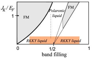
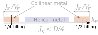
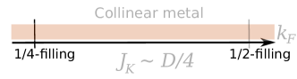
Figure 1: (color on-line) The upper panel: a cartoon illustrating the weak and the moderate coupling regimes of the phase diagram obtained numerically for 1D KL in Ref.McCulloch et al. (2002). The two shaded regions are ferromagnetic phases. The region called “Polaronic Liquid” corresponds to the large Fermi surface whose volume incorporates both conduction and localized electrons. The Kondo effect is suppressed in all regions. The orange box marks the range of parameters considered in the present paper. The central and the lower panels: phase diagrams of 1D KL obtained for small $J_{K}/E_{F}$, see explanations in Sect.IV

The position of the maximum in the momentum-dependent structure factor of the spins is different above and below this intermediate ferromagnetic region. At larger $J_{K}$, the maximum is located at $\pi/\xi-2k_{F}$, with $k_{F}$ being the Fermi momentum of the band electrons. Such peak position corresponds to the scenario where both the local moments and the conduction electrons contribute to the Fermi surface (FS) volume (the so-called large FS). On the other hand, at small $J_{K}$, the maximum is at $2k_{F}$. It was suggested in Ref.McCulloch et al. (2002) that this corresponds to the small FS. However, we will argue that the state at a generic filling is $4k_{F}$-Charge Density Wave (CDW) with short range spin fluctuations centered at $2k_{F}$. The Friedel oscillations at $4k_{F}$ do not distinguish between large and small FS. The large FS has been also found in the recent Density Matrix Renormalization Group study conducted away from 1/4, 3/4 and 1/2 fillings for the relatively large $J_{K}$, Ref.Khait et al. (2018). The authors of this paper have reported existence of a heavy Tomonaga-Luttinger liquid (TLL) with gapless charge and spin excitations and Friedel oscillations at $k_{F}^{*}=\pi/2\xi-k_{F}$.

We will argue that the RKKY interaction generically dominates in 1D dense KLs. For KLs with magnetic anisotropy, it has been demonstrated in our previous publications Schimmel et al. (2016); Tsvelik and Yevtushenko (2015) for the case of incommensurate filling. Ref.Schimmel et al. (2016) contains Renormalization Group arguments which demonstrate suppression of the Kondo effect.

The Kondo effects can dominate in the 1D KL only under some specific conditions, e.g. for small concentrations of local moments, strongly broken SU(2) spin-rotation symmetry and strong Coulomb interactions Yevtushenko and Yudson (2018) or strongly enlarged symmetry (SU($N$) instead of SU(2) with $N\gg 1$) Shibata et al. (1997).

The surest indication of the RKKY-dominated physics is that it is insensitive to the sign of $J_{K}$ but, at the same time, is very sensitive to doping and anisotropy of the Kondo coupling. For example: (i) KL at half-filling is an insulator with gapped or critical spin excitations; (ii) at quarter-filling, KL is also an insulator but with a strong tendency for spin dimerization, which agrees with the numerical study reported in Ref.Xavier et al. (2003); (iii) at incommensurate filling, KL with generalized SU(N) symmetry for large $N\gg 1$ has been predicted to be TLL Shibata et al. (1997); (iv) the anisotropic incommensurate KL is also described by TLL either with a spin-charge separation (easy-axis anisotropy) or with a separation of different helical sectors (easy-plane anisotropy) Tsvelik and Yevtushenko (2015); Schimmel et al. (2016). The latter phase is characterized by broken helical symmetry of fermions which governs a partial protection of ballistic transport against effects of disorder and localization. We remind the readers that helicity of 1D electrons is defined as the sign of the product of their spin and chirality.

We will consider the isotropic case with SU(2) symmetry and, thus, complete the picture of the RKKY dominated physics in the dense 1D KL. Many of the prominent features of 1D KL have been observed only in numerical studies. The goal of the present paper is to develop an analytical approach for the region of $J_{K}/E_{F}\ll 1$, see Fig.1, where numerical calculations are difficult to perform, but analytical methods become very powerful. By utilizing various field-theoretical methods, we have developed a fully analytical and controlled description of the dense 1D KLs at arbitrary doping. We will show below that 1D KL can form three distinct phases: (i) the insulator at special commensurate fillings, or (ii) a usual metal formed by interacting electrons when the band filling is close to the special commensurate fillings, or (iii) $4k_{F}$-charge-density-wave (CDW) state with gapped spin excitations. Remarkably, the third phase can also be described as a metal where the transport is carried by helical Dirac fermions. We have determined conditions under which one or another conducting phase appears. In particular, interacting spinful fermions (either a Fermi liquid or TLL) always exist close to the commensurate insulator and form a usual 1D metal. If the Kondo coupling is relatively large, this phase exists at any generic filling and becomes the heavy TLL.

The $4k_{F}$-CDW phase with helical transport can exist only at $J_{K}\ll E_{F}$ far from the commensurate insulator. Therefore, it can be detected only when parameters are properly tuned. On the other hand, it is very notable because it possesses an emergent protection against disorder and localization. The emergent protection caused by interactions is well known and attracts ever-growing attention of theoreticians Pershin et al. (2004); Braunecker et al. (2009a, b, 2010); Kloeffel et al. (2011); Klinovaja et al. (2011a, b, 2012); Kainaris and Carr (2015); Tsvelik and Yevtushenko (2015); Schimmel et al. (2016); Pedder et al. (2016); Kainaris et al. (2017), and experimentalists Quay et al. (2010); Scheller et al. (2014); Kammhuber et al. (2017); Heedt et al. (2017). To the best of our knowledge, all previously known examples were found in the systems with broken (either spontaneously or at the level of the Hamiltonian) SU(2)-symmetry. Our finding is novel from this point of view because we predict such a protection to appear in the rotationally invariant system.

We note in passing that, a competition of the RKKY interaction with a direct Heisenberg exchange in dense 1D KL introduces additional level of complexity and can lead to appearance of exotic phases with a nontrivial spin order, such as a chiral spin liquid Tsvelik and Yevtushenko (2017) or a chiral lattice supersolid Yevtushenko and Tsvelik (2018).

The rest of the paper is organized as follows: Section II describes the model used in our study. Separation of fast and slow variables is explained in Section III. Section IV contains a brief and non-technical summary of our results at the level of mean-field approximation. Section V is more technical as it is devoted to the detailed field theoretical description of all phases in KL. In Section VI, we discuss possible numerical studies and experiments related to our theory. Section VII contains conclusions. Technical details are presented in Appendices.

The mean field analysis and the protected transport in the $4k_{F}$-CDW phase are addressed in detail in Ref.Tsvelik and Yevtushenko (2019). In the present paper, we concentrate mainly on the quantum theory which allows us to analyze the phase diagram of the KL. Repetition of results reported in Ref.Tsvelik and Yevtushenko (2019) is reduced here to a minimum necessary to make the paper self-contained.

II The model

We start from the standard KL Hamiltonian:

$$\hat{H}=\sum_{n}\Big{[} - t\left(\psi^{\dagger}_{n}\psi_{n+1}+h.c.\right)-\mu\,\psi^{\dagger}_{n}\psi_{n}+$$

$$+ J_{K}\psi_{n}^{\dagger}({\bm{\sigma}},{\bm{S}}_{n})\psi_{n}\Big{]},$$

where $\psi_{n}\equiv\{\psi_{n,\uparrow},\psi_{n,\downarrow}\}^{\rm T}$  are electron annihilation ($\psi^{\dagger}_{n}$ - creation) spinor operators; ${{\bm{S}}}_{n}$ are quantum spins with magnitude $s$; ${\bm{\sigma}}\equiv\{\sigma_{x},\sigma_{y},\sigma_{z}\}$ are Pauli matrices in the spin space; $t$ and $\mu$ are the electron hopping and the chemical potential, respectively; summation runs over lattice sites. For simplicity, we do not distinguish constants of KI and crystalline lattices, $\xi_{s}=\xi$. We also assume that $sJ_{K}\ll D$ where $D=2t$ and consider only low temperatures, $T\to 0$.

III Separating slow
and fast variables

We are going to derive an effective action for the low energy sector of the theory. The crucial step is to single out smooth modes. It is technically convenient to restrict ourselves to the case $|\mu|,~{}|J_{K}|\ll t$ which allows us to linearize the dispersion relation and introduce right- and left moving fermions, $\psi_{\pm}$, in a standard way Giamarchi (2004). In the continuous limit, the fermionic Lagrangian density takes the form

$${\cal L}_{F}[\psi_{\pm}]=\sum_{\nu=\pm}\psi^{\dagger}_{\nu}\partial_{\nu}\psi_{\nu}\,;\quad\partial_{\pm}\equiv\partial_{\tau}\mp iv_{F}\partial_{x}\,.$$ (2)

Here $v_{F}$ is the Fermi velocity, $\nu$ is the chiral index which indicates the direction of motion, $\partial_{\nu}$ is the chiral derivative and $\tau$ is the imaginary time.

Following Refs.Tsvelik (1994); Tsvelik and Yevtushenko (2015); Schimmel et al. (2016), we keep in the electron-KI interaction only backscattering terms which are the most relevant in the case of the dense 1D KL. The part of the electron-KI interaction describing the backscattering on the site $n$ reads as:

$${\cal L}_{\rm bs}(n) = J_{K}\left[R^{\dagger}_{n}({\bm{\sigma}},{\bm{S}}_{n})L_{n}e^{-2ik_{F}x_{n}}+h.c\right];$$ (3)

$$R \equiv \psi_{+},\,L\equiv\psi_{-}\,;\ x_{n}\equiv n\xi.$$

At large inter-impurity distance, the backscattering with a spin flip is a part of the Kondo screening physics. However, as we show below, the physics of dense KL is quite different. This will be proven by insensitivity of all answers to ${\rm sign}(J_{K})$. The Kondo screening is suppressed in our model if $T_{K}\ll J_{K}\ll v_{F}/\xi$. The second inequality is important to accomplish separation of the fast and the slow modes Tsvelik and Yevtushenko (2015); Schimmel et al. (2016).

${\cal L}_{\rm bs}(n)$ contains fast $2k_{F}$-oscillations which must be absorbed into the spin configuration. We perform this step in the path integral approach where the spin operators are replaced by integration over a normalized vector field. We decompose this field as

$${\bm{S}}_{n}/s={\bm{m}}+b\Big{(} {\bm{e}}_{1} \,\cos(\alpha)\cos(qx_{n}+\theta)+$$

$${\bm{e}}_{2} \,\sin(\alpha)\sin(qx_{n}+\theta)\Bigr{)}\sqrt{1-{\bm{m}}^{2}}\,.$$

where $q\simeq 2k_{F}$, $\theta$ is a constant (coordinate independent) phase shift; $\{{\bm{e}}_{1},{\bm{e}}_{2},{\bm{m}}\}$ with $|{\bm{e}}_{1,2}|=1$ is an orthogonal triad of vector fields whose coordinate dependence is smooth on the scale $1/k_{F}$. The constant $b$ and the angle $\alpha$ must be chosen to solve normalization $|{\bm{S}}/s|=1$. Eq.(III) is generic and it allows only for three possible choices of $b$, $\alpha$ and $\theta$ determined by the band filling: either 1/2, $qx_{n}=2k_{F}x_{n}=\pi n\Rightarrow b=1,\,\theta=\alpha=0$, or 1/4, $qx_{n}=2k_{F}x_{n}=\pi n/2\Rightarrow b=\sqrt{2},\ \theta=\pi/4$, or a generic one, $b=\sqrt{2},\ \theta=0,\ \alpha=\pi/4\$ Tsvelik and Yevtushenko (2019).

Using the machinery of advanced field-theoretical methods becomes easier if the vectors ${\bm{e}}_{1,2}$ are expressed via a matrix $g\in\mbox{SU(2)}$

$${\bm{e}}_{1,2,3}=\frac{1}{2}{\rm tr}[{\bm{\sigma}}g\sigma_{x,y,z}g^{-1}]\,;$$ (5)

see Appendix A. $g$ is a smooth function of $x$ and $\tau$ and it governs new rotated fermionic basis

$$\tilde{R} \equiv g^{-1}R,\ \tilde{L}\equiv g^{-1}L\,;$$ (6)

$${\cal L}_{F}[\tilde{R},\tilde{L}] = \tilde{R}^{\dagger}(\partial_{+}+g^{-1}\partial_{+}g)\tilde{R}+\tilde{L}^{\dagger}(\partial_{-}+g^{-1}\partial_{-}g)\tilde{L}.$$

Jacobian of this rotation is given in Appendix B.

Now we insert Eq.(III) into Eq.(3), select non-oscillatory parts of ${\cal L}_{\rm bs}$ for three above mentioned cases, and take the continuous limit. This yields the smooth part of the Lagrangian density:

$${\cal L}_{\rm bs}^{(1/2)}\! = \!\tilde{J}\sqrt{1-{\bm{m}}^{2}}\left(\tilde{R}^{\dagger}\sigma_{x}\tilde{L}+h.c\right);$$ (7)

$${\cal L}_{\rm bs}^{(1/4)}\! = \!\frac{\tilde{J}\sqrt{1-{\bm{m}}^{2}}}{\sqrt{2}}\Bigl{(}e^{i\pi/4}\tilde{R}^{\dagger}[\cos(\alpha)\sigma_{x}+i\sin(\alpha)\sigma_{y}]\tilde{L}+$$ (9)

$$\qquad\qquad\qquad+\,h.c\Bigr{)};$$

$${\cal L}_{\rm bs}^{\rm(gen)}\! = \!\tilde{J}\sqrt{1-{\bm{m}}^{2}}\left(\tilde{R}^{\dagger}\sigma_{-}\tilde{L}+h.c\right).$$ (10)

Here the superscript of $\cal{L}_{\rm bs}$ denotes the band filling; $\tilde{J}\equiv sJ_{K}/2$, and $\sigma_{\pm}=(\sigma_{1}\pm i\sigma_{2})/2$. Note that the low energy physics of KLs with the 1/4- and 3/4-filling is equivalent in our model. Therefore, we often discuss only quarter-filling in the text and do not repeat the same discussion for the case of the 3/4-filling.

One can give the following interpretations to the above introduced spin configurations: Eq.(7) corresponds to a staggered configuration of spins at half-filling, $\uparrow\downarrow$, which was studied in Ref.Tsvelik (1994). Eq.(9) assumes two spins up- two spins down configuration, $\uparrow\uparrow\downarrow\downarrow$, which agrees with the spin dimerization tendency observed numerically in Ref.Xavier et al. (2003) at quarter-filling. Eq.(10) is a rotationally invariant counterpart of the helical spin configuration discovered in Refs.Tsvelik and Yevtushenko (2015); Schimmel et al. (2016) in the anisotropic KL at incommensurate fillings. A simplified version of the spin configuration Eq.(10) was used also in Ref.Fazekas and Müller-Hartmann (1991) for analyzing the phase diagram of KL at the level of the mean field approximation. We emphasize, however, that our approach is more advanced and generic since it has allowed us to go much further, namely, to derive the low energy effective action and to take into account quantum fluctuations for all phases.

Backscattering of the Dirac fermions $\{\tilde{R},\tilde{L}\}$ opens a gap, $\Delta\propto\tilde{J}\sqrt{1-{\bm{m}}^{2}}$, in their spectrum. If the gap is opened at (or close to) the Dirac point, defined by the level of the chemical potential, it decreases the ground state energy of the fermions see Fig.2a–d. The larger the gap, the stronger is the gain in the fermionic energy:

$$\delta E_{\rm GS}=-\vartheta_{0}\,\xi\sum_{k=1,2}\Delta^{2}_{k}\log\bigl{(}D/|\Delta_{k}|);$$ (11)

see Eqs.(12–14) below and Ref.Tsvelik and Yevtushenko (2019). Here, $\vartheta_{0}=1/\pi v_{F}$ is the density of states of the 1D Dirac fermions and the sum runs over two fermionic (helical) sectors.

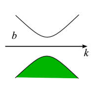
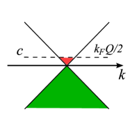
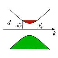
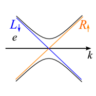
Figure 2: (color on-line) Panels (a) and (b): the ground state of fermions $\tilde{R},\tilde{L}$ with zero chemical potential (green region) before and after opening of the gap at the level of $\mu$. Panels (c) and (d): the ground state of the fermions for the case of a finite positive chemical potential. The red regions mark the states between the gap and the chemical potential which can form Tomonaga-Luttinger liquid. Panel (e) exemplifies a co-existence of the gapped (black lines) and the gapless (orange and blue lines) helical fermions.

Since the spin degrees of freedom do not have kinetic energy the minimum of the ground state energy is reached at the maximum of the fermionic gap. This indicates that $|{\bm{m}}|$ is the gapped variable and has the classical value $m_{0}=0$.

IV Mean-field analysis

Let us for the moment neglect all quantum fluctuations and briefly repeat the mean–field analysis which has been presented in Ref.Tsvelik and Yevtushenko (2019). The KL contains two fermionic sectors which can have different gaps depending on the band filling and the spin configuration. The gaps can be found from Eqs.(7-10):

$${\cal L}_{\rm bs}^{\rm(1/2)}: \Delta^{(1/2)}_{1,2}=\tilde{J};$$ (12)

$${\cal L}_{\rm bs}^{\rm(1/4)}: \Delta^{(1/4)}_{1,2}=\tilde{J}(\cos(\alpha)\pm\sin(\alpha))/\sqrt{2};$$ (13)

$${\cal L}_{\rm bs}^{\rm(gen)}: \Delta^{\rm(gen)}_{1}=\tilde{J},\ \Delta^{\rm(gen)}_{2}=0.$$ (14)

At special commensurate fillings, the minimum of the ground state energy is provided by those spin configurations which open the gaps at the Dirac point of both fermionic sectors, i.e., by the commensurate configurations Eq.(7) and Eq.(9) [with $\alpha=0,\pi/2$] for the 1/2- and 1/4-filling, respectively. Note that $\alpha$ is gapped at quarter-filling. The conduction band of these commensurate KLs is empty (see Fig.2b) and, hence, they are insulators, as expected.

The commensurate spin configurations minimize the ground state energy also in a vicinity of half- and quarter fillings. This means that the wave vector $q$ of the spin modes remains commensurate, Eqs.(7,9), and is slightly shifted from $2k_{F}$: $2k_{F}-q\equiv Q\ll 1/\xi$. This case can be described in terms of backscattered Dirac fermions which, unlike the standard approach describing 1D systems, have non-zero chemical potential:

$$\bar{{\cal L}}={\cal L}_{F}[R,L]+{\cal L}_{\rm bs}^{(f)}[R,L]-(v_{F}Q/2)(R^{\dagger}R+L^{\dagger}L),$$ (15)

where $f=1/4,1/2$. To be definite we analyze upward shift of the chemical potential, see Fig.2c, downward shift can be studied in much the same way. Backscattering caused by the commensurate spin configuration opens the gap which is now slightly below the level of $\mu$. The states with energies $0<E\leq v_{F}Q/2$ are pushed above the gap, see Fig.2d. These electrons have almost parabolic dispersion:

$$E^{+}(k)\bigl{|}_{v_{F}|k|<|\tilde{J}|}\simeq|\tilde{J}|+\left(v_{F}k\right)^{2}/2|\tilde{J}|\,.$$ (16)

Since this new phase possesses a partially filled band it is a metal. Its metallic behavior originates from the spin configuration whose classic component is governed by only one slowly rotating vector, e.g. ${\bm{e}}_{1}$, and, therefore, is close to the collinear one. We will reflect this fact by referring to such phases as “collinear metals” (CMs).

The CM becomes less favorable phase when $|Q|$ increases. This is obvious from Fig.2: the potential energy of the electrons in the upper band

$$E_{\rm p}\simeq\xi\tilde{J}k_{F}^{*}/\pi+\xi v_{F}^{2}(k_{F}^{*})^{3}/6\pi\tilde{J}\,;$$

becomes large when $k_{F}^{*}=Q/2$ increases . If $|Q|$ is large enough

$$|Q|>Q_{c}\sim\tilde{J}/v_{F}\,.$$ (17)

the minimum of the ground state energy is provided by the general spin configuration, Eq.(10). We would like to emphasize that the spin configuration cannot change gradually. The switching from the commensurate to the generic configuration is always abrupt and, therefore, $Q_{c}$ is the point of a quantum phase transition.

If $\tilde{J}/v_{F}\ll 1/\xi$, there is always a parametrically large window of the band fillings where the new phase is realized instead of the CM, see the central panel of Fig.1. In the opposite case of large $\tilde{J}$, this window shrinks to zero and the CM dominates at all fillings excluding two special commensurate cases 1/2 and 1/4, see the lower panel of Fig.1. This allows us to surmise that the CM, which we have predicted, corresponds to the “polaronic liquid” reported in Ref.McCulloch et al. (2002) for the case $J_{K}\sim E_{F}$. The detailed theory of KL with large $J_{K}$ is beyond the scope of the present paper.

The remaining case of generic filling, Eq.(10), is the most prominent for transport because rotated fermions are gapped only in one helical sector, e.g. $\tilde{R}_{\downarrow},\tilde{L}_{\uparrow}$, and the second helical sector, $\tilde{R}_{\uparrow},\tilde{L}_{\downarrow}$, remains gapless, see Eq.(14) and Fig.2e. This means that the helical symmetry of the fermions $\tilde{R},\tilde{L}$ is broken on the mean-field level. On the other hand, the rotating matrix $g$ slowly changes in space and time and, therefore, the spin configuration can be characterized only as a local helix. To reflect this, we refer to the KLs with the locally broken as helical metals (HMs). It has been shown in Ref.Tsvelik and Yevtushenko (2019) that the HMs inherit the symmetry protection of those KLs where the helical symmetry is broken globally Tsvelik and Yevtushenko (2015); Schimmel et al. (2016), see also the discussion in the next Section.

V Quantum-mechanical theory

Before presenting the quantum-mechanical approach, let us summarize its key steps. Firstly, we integrate out gapped fermions, exponentiate the fermionic determinant as $\rm{Tr}\log[\hat{G}_{0}^{-1}+\hat{\cal G}+\delta\hat{\Delta}]$, with

$$\hat{G}_{0}^{-1}=\left(\begin{array}[]{cccc}\partial_{+}&0&0&\Delta_{2}\\ 0&\partial_{+}&\Delta_{1}&0\\ 0&\Delta_{1}&\partial_{-}&0\\ \Delta_{2}&0&0&\partial_{-}\end{array}\right);$$ (18)

describing the fermions in the case of the classical configuration of spins. Spin and gap fluctuations are contained in matrices $\hat{\cal G}={\rm diag}(g^{-1}\partial_{+}g,g^{-1}\partial_{-}g)$ and $\delta\hat{\Delta}$ respectively; detailed definitions are given in Appendix C. To derive the effective theory, we add to the exponentiated determinant the Jacobian of the SU(2) rotation and expand obtained Lagrangian in gradients of the matrix $g$ and in small fluctuations of $|m|$ around its classical value $m_{0}=0$. The commensurate spin configuration, which corresponds to 1/4-filling, requires also the expansion in fluctuations of $\alpha$.

Next, we reinstate the Wess-Zumino term for the spin field Tsvelik (2003), which is required by the quantum theory:

$${\cal L}_{\rm WZ}=is\int_{0}^{1}{\rm d}u\,({\bm{N}},[\partial_{u}{\bm{N}}\times\partial_{\tau}{\bm{N}}])\,;$$ (19)

where $u$ is an auxiliary variable, ${\bm{N}}(u=1)={\bm{S}}/s$ and ${\bm{N}}(u=0)=(1,0,0)$. We insert the decomposition Eq.(III) into Eq.(19) and select non-oscillating parts of ${\cal L}_{\rm WZ}$. The commensurate spin configurations generate also the topological term (see Ref.Tsvelik (1994), Sect.16 of the book Tsvelik (2003), and references therein).

Finally, we integrate out fluctuations of $|m|$ (and of $\alpha$, if needed) in the Gaussian approximation.

These steps result in the nonlinear $\sigma$-model (nLSM) in 1+1 dimensions, which describes the spin degrees of freedom. We will argue that the theory which we suggest is stable.

The nLSM depends on the band filling. Its derivation is rather lengthy but standard. Therefore, we will present in the main text only answers and explain the algebra in Appendices C–F.

V.1 Insulating KL at special commensurate fillings

The Lagrangian of $\sigma$-model at the special commensurate fillings takes the following form:

$${\cal L}^{(f)}=\frac{1}{2g_{f}}\left[\frac{(\partial_{\tau}{\bm{e}}_{1})^{2}}{c_{f}}+c_{f}(\partial_{x}{\bm{e}}_{1})^{2}\right]\,;$$ (20)

where “$f$” denotes the band filling, either 1/2 or 1/4, $c_{f}=v_{F}g_{f}/4\pi$ is the normalized velocity of the spin excitations and $g_{f}$ is the dimensionless coupling constant:

$$g_{1/2} = 4\pi/\sqrt{1+s^{2}/(\vartheta_{0}\xi\tilde{J})^{2}\log[D/|\tilde{J}|]}\,;$$ (21)

$$g_{1/4} = 4\pi/\sqrt{1+8s^{2}/(\vartheta_{0}\xi\tilde{J})^{2}\log[\sqrt{2}D/|\tilde{J}|]}\,.$$

Clearly, the $\sigma$-model contains only one vector, ${\bm{e}}_{1}$ in our choice of variables, which governs the fermionic gap. The second vector, ${\bm{e}}_{2}$, is redundant in the case of the special commensurate fillings.

The action is given by the sum of the gradient- and topological terms:

$$S^{(f)}=\int{\rm d}\tau{\rm d}x{\cal L}^{(f)}+S_{\rm top},\ S_{\rm top}=(2s-1)i\pi k\,.$$ (22)

The integer $k$ marks topologically different sectors of the theory.

Hence, the spin excitations at the special commensurate cases are described by the O(3)-symmetric nLSM in (1+1) dimensions with the topological term. Its spectrum depends on the value of $2s-1$: half-integer $s$ are all equivalent to zero topological term and integer ones to $S_{\rm top}=i\pi$. The O(3) nonlinear sigma model is exactly solvable in both cases Wiegmann (1985); Fateev and Zamolodchikov (1991); Tsvelik (2003). It possesses a characteristic energy scale

$${\cal E}_{f}\sim|\tilde{J}|g_{f}^{-1}\exp(-2\pi/g_{f}),\ f=1/2,1/4\,.$$ (23)

For half-integer $s$, this scale is the spectral gap of the coherent triplet excitations whose dispersion has a relativistic form:

$$\mbox{half-integer $s$}:\quad\epsilon_{f}(p)=\sqrt{{\cal E}_{f}^{2}+(c_{f}p)^{2}}.$$ (24)

For integer $s$, ${\cal E}_{f}$ marks a crossover from the weak coupling regime to a critical state [in the field-theoretical language, it is described by the SU₁(2) Wess-Zumino-Novikov-Witten theory with central charge $C=1$]. Below ${\cal E}_{f}$, such KL behaves as spin-1/2 Heisenberg antiferromagnet with incoherent spin response and gapless excitation spectrum consisting of spin-1/2 spinons.

We note that, for small $\tilde{J}$, the energy scale ${\cal E}_{f}$ is exponential in $1/|\tilde{J}|$ and, for $\tilde{J}>0$, it may be confused with the Kondo temperature. However, as we have mentioned above, ${\cal E}_{f}$ does not depend on the sign of $\tilde{J}$ which testifies to the fact that the underlying physics is related to the RKKY exchange and not to the Kondo screening.

V.2 KL in a vicinity of special commensurate fillings

We have explained already that the spin configuration remains unchanged if the band filling is slightly detuned from one of the special commensurate cases. The novel features of such KLs are caused by the presence of the conduction electrons. They are coupled to spin modes which can mediate indirect electron interaction. In the rotated fermionic basis, the electron-spin coupling is described by

$${\cal L}_{\rm e-s}=\tilde{R}^{\dagger}g^{-1}\partial_{+}g\tilde{R}+\tilde{L}^{\dagger}g^{-1}\partial_{-}g\tilde{L}\,$$ (25)

(see Eq.(6) and the first paragraph in Appendix C). The energy of the effective electron interaction can be estimated (at least for the case of the gapped spin excitations) after selecting in Eq.(25) the contribution of the only relevant vector ${\bm{e}}_{1}$

$$g\to i({\bm{\sigma}},{\bm{e}}_{1}),\quad g^{-1}\partial_{\alpha}g\to i\bigr{(}{\bm{\sigma}},[{\bm{e}}_{1}\times\partial_{\alpha}{\bm{e}}_{1}]\bigl{)}\,;$$

(see Appendix A), neglecting time derivatives, and integrating over $\partial_{x}{\bm{e}}_{1}$. This yields:

$${\cal L}^{\rm(eff)}_{\rm e-e}\sim-\bigl{[}(\tilde{R}^{\dagger}{\bm{\sigma}}\tilde{R})^{2}+(\tilde{L}^{\dagger}{\bm{\sigma}}\tilde{L})^{2}\bigr{]}/\vartheta_{0}\,.$$ (26)

Thus, for the dressed fermions, we obtain a strongly repulsive Fermi gas. In the energy range close to the new Fermi surface, $|E-E^{+}(k_{F}^{*})|\ll E^{+}(k_{F}^{*})$, the effective interaction converts the conduction electrons to the repulsive and spinful TLL whose excitations are charge and spin density waves. This TLL is characterized by a new Fermi momentum $k^{*}_{F}=Q/2=k_{F}-\pi/2\xi$ near 1/2-filling or $k^{*}_{F}=Q/2=k_{F}-\pi/4\xi$ near 1/4-filling. If the effective repulsion is strong enough, TLL becomes heavy. In particular, the velocity of CDW becomes much smaller than $v_{F}$. Such a heavy TLL has been observed numerically in Ref.Khait et al. (2018).

The spin response of the conduction electrons is shifted to the region of wave vectors between 0 and $2k_{F}^{*}$ while the main response of the spin sector is at frequencies higher than the spin gap coming from the vicinity of the commensurate wave vector ($\pi/\xi$ for half filling, $\pm\pi/2\xi$ for quarter filling), see a cartoon in Fig.3.

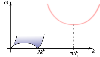
Figure 3: (color on-line) The spin response of the KL close to the special commensurate fillings. The main response is at frequencies higher than the spin gap and coming from the vicinity of the commensurate wave vector (e.g., $\pi/\xi$ for half filling). The spin response of TLL is shifted to the region of wave vectors between 0 and $2k_{F}^{*}$

The appearance of the new Fermi vector $k^{*}_{F}$ points to the existence of the large FS. The response at $2k_{F}$ is suppressed and is replaced by the singular response at $2k^{*}_{F}$ in agreement with the general theory Yamanaka et al. (1997); Oshikawa (2000). Note that 1D nature and the effective repulsion make CMs very sensitive to spinless impurities: even a weak disorder easily drives it to the Anderson localized regime with suppressed dc transport Giamarchi and Schulz (1988).

V.3 KL at arbitrary fillings

The Lagrangian of the $\sigma$-model at the generic band filling takes the following form:

$${\cal L}^{\rm(gen)}=\frac{1}{2g_{\rm gen}}\left\{\frac{\left[\Omega_{\tau}^{(z)}\right]^{2}}{c_{\rm gen}}+c_{\rm gen}{\rm tr}(\partial_{x}g^{+}\partial_{x}g)\right\}\,;$$ (27)

with

$$g_{\rm gen}=\pi/\sqrt{1+8s^{2}/(\vartheta_{0}\xi\tilde{J})^{2}\log[D/|\tilde{J}|]}$$ (28)

and $c_{\rm gen}=v_{F}g_{\rm gen}/\pi,\ \Omega_{\tau}^{(z)}\equiv i{\rm tr}[\sigma_{z}g^{-1}\partial_{\tau}g]/2$. This theory is anisotropic and has only the SU(2)-symmetry, $g\to{\cal M}g,\,{\cal M}\in\mbox{ SU(2)}$. Moreover, the time derivative is present only in the $\Omega^{z}$ term. This points to a short correlation length of spins and may challenge our approach, which is based on separation of the fast and the slow degrees of freedom in the spin dynamics. However, the $\sigma$-model Eq.(27) has been derived for scales larger than the coherence length of the gapped fermions, $v_{F}/\Delta^{\rm(gen)}\gg\xi$. Thus, the actual UV cut-off of the theory is much larger than the lattice spacing and the working hypothesis on the scale separation is not violated. The spin gap is expected to be $\propto\Delta^{\rm(gen)}\sim\tilde{J}$. More detailed analysis of the spin dynamics in this generic phase will be present elsewhere.

The gapped spins mediate repulsion between the gapless electrons. Its strength can be estimated similar to the CM case.

Let us now identify the nature of the HM in terms of its low energy excitations. First, we note that the fermion density, current density and backscattering operators are invariant under $g$-rotation (6):

$$R^{\dagger}R=\tilde{R}^{\dagger}\tilde{R},\ L^{\dagger}L=\tilde{L}^{\dagger}\tilde{L},\ R^{\dagger}L=\tilde{R}^{\dagger}\tilde{L}\,.$$ (29)

The low energy physics is governed by fields whose correlation functions decay as power law. To obtain them, we project the fields on the gapless sector, i.e., average over high-energy gapped modes. For example, components of the charge density are:

$$q\simeq 0: \rho_{0}=\tilde{R}^{\dagger}_{\uparrow}\tilde{R}_{\uparrow}+\tilde{L}^{\dagger}_{\downarrow}\tilde{L}_{\downarrow}\,;$$ (30)

$$q\simeq 4k_{F}: \rho_{4k_{F}}=e^{-4ik_{F}x}\tilde{R}^{\dagger}_{\uparrow}\langle\tilde{R}^{\dagger}_{\downarrow}\tilde{L}_{\uparrow}\rangle\tilde{L}_{\downarrow}+h.c.$$ (31)

The absence of $\rho_{2k_{F}}$ has a simple physical explanation: it would correspond to a single particle elastic backscattering between the gapless fermion and the gapped one which is not allowed. The same argument was used to omit contributions to $\rho_{4k_{F}}$ which are not included in Eq.(31). Since the projection of the spin density on the low energy sector vanishes, the helical metal is the $4k_{F}$-CDW phase. This fact has two important consequences: (i) the (local) spin helix moves the Friedel oscillations of the charge density from $\,2k_{F}\,$ to $\,4k_{F}\,$, which is indistinguishable from $\,4(k_{F}-\pi/2\xi)\,$ due to $k$-periodicity; and, even more importantly, (ii) it drastically reduces backscattering caused by spinless disorder, see Ref.Tsvelik and Yevtushenko (2019) for details.

VI Discussion of further
numerical and experimental studies
of Kondo Lattices

The insulating KLs were studied numerically in several papers, for example, in Ref.Xavier et al. (2003) (1/4-filling) and Ref.Huang et al. (2019) (3/4-filling). A very important task for the subsequent research is to reliably detect different metallic phases in 1D KL. This requires to tune system parameters, in particular, the band filling and the Kondo coupling. Detecting the CM is a relatively simple task because it is generic at relatively large $J_{K}$ and filling away from 1/2, 1/4 and 3/4. The heavy TLL formed by the interactions in the CM has been observed in the numerical results of Ref.Khait et al. (2018). However, $J_{K}$ was too large for finding the HM. The KL studied in Ref.Smerat et al. (2011) exhibits an unexpected $2k_{F}$-peak at small $J_{K}$. Yet, the peak was detected in the spin susceptibility of 6 fermions distributed over 48 sites. So small KL cannot yield a conclusive support or disproof of our theory. A more comprehensive study of the larger KLs is definitely needed.

We have already described conditions under which one or other metallic phase appears. Here, we would like to recapitulate their key features which could help to distinguish these phases in numerics and in experiments. The conductance of the CM is equal to the quantum $G_{0}=2e^{2}/h$ while the HM must show only $G_{0}/2$ conductance due to the lifted spin degeneracy. CM is a spinful TLL. Its response has a peak at the shifted Fermi momentum. HM must possess the same property Yamanaka et al. (1997); Oshikawa (2000). However, HM is $4k_{F}$-CDW and, therefore, $k_{F}$ and $k_{F}^{*}$ are indistinguishable on the lattice. This indicates that HM has the response peak at $k_{F}$. Since CM responds to scalar potentials at $2k_{F}^{*}$ and HM – at $4k_{F}^{*}\equiv 4k_{F}$, the spinless disorder potential may have a profound difference with respect to the transport in the CM and HM phases. Namely, localization is parametrically suppressed in HM.

The best control of the system parameters is provided by the experimental laboratory of cold atoms where 1D KL was recently realized Riegger et al. (2018). Such experiments are, probably, the best opportunity to test our theory. However, modern solid-state technology also allows one to engineer specific 1D KL even in solid state platforms. It looks feasible to fabricate 1D KL in clean 1D quantum wires made, e.g., in GaAs/AlGaAs by using cleaved edge overgrowth technique Pfeiffer et al. (1993) or in SiGe Mizokuchi et al. (2018). Magnetic ad-atoms can be deposited close to the quantum wire with the help of the precise ion beam irradiation. One can tune parameters of these artificial KLs by changing the gate voltage, type and density of the magnetic ad-atoms and their proximity to the quantum wire. The experiments should be conducted at low temperatures, $T\ll\Delta,{\cal E}$, where destructive thermal fluctuations are weak.

As far as more conventional condensed matters systems are concerned, we are aware of only one group of candidates: the quasi-one-dimensional organic compounds Per₂M(mnt)₂ (M =Pt, Pd). They are considered as realizations of weakly coupled quarter-filled S=1/2 Kondo chains Henriques et al. (1984, 1986); Bourbonnais et al. (1991); Matos et al. (1996); Green et al. (2011); Pouget et al. (2017), although the role of the interchain coupling there is not clear. According to Refs. Henriques et al. (1984, 1986); Bourbonnais et al. (1991); Matos et al. (1996); Green et al. (2011), (Per)₂[Pt(mnt)₂] possesses a unique combination of Spin-Peierls and CDW order parameters, which agrees with our theory. The band in the perylene chain is quarter-filled and the band in the Pt(mnt)₂ chain is half-filled Henriques et al. (1986); Alcácer et al. (1980). The perylene chain is metallic, and at low temperature undergoes a Peierls (CDW) transition to an insulating state where the perylene molecules tetramerize with wave vector $q_{\rm Per}=\pi/2\xi$. The Pt(mnt)₂ chain is an insulator that undergoes a spin-Peierls transition where the Pt-dithiolate molecules dimerize with wave vector $q_{\rm Pt}=\pi/\xi$; here the spin-1/2 Pt moments form a spin-singlet. Remarkably, even though $q_{\rm Pt}=2q_{\rm Per}$, diffuse x-ray scattering, specific heat, and electrical transport measurements indicate that both the CDW and SP transitions occur at the same, or very similar temperature Gama et al. (1993); Bonfait et al. (1993). This observation suggests that the two chains are strongly coupled in spite of the mismatch in q-vectors.

VII Conclusions

We have developed a unified theory for 1D Kondo lattice with a dense array of spins in the regime of a small and rotationally invariant Kondo coupling, $|J_{K}|\ll E_{F}$. The physics of such KLs is controlled by the RKKY indirect spin interaction. This is clearly demonstrated by the fact that their low energy properties are insensitive to the sign of the Kondo exchange. Nevertheless, the phase diagram is quite rich. We have identified three different phases. They include (i) the insulating phase which appears at special commensurate band filling, either 1/2, or 1/4, 3/4; (ii) spinful interacting metals which exist in the vicinity of that commensurate fillings; and (iii) $4k_{F}$ Charge Density Wave phase at generic band fillings, see Fig.(1). Electron-spin interactions can convert the 2nd phase to the heavy Tomonaga-Luttinger liquids.

Spin configurations, which govern the 1st and the 2nd phases, are collinear. That’s why the second phase can be called “collinear metal”. The spin fluctuations around these classical arrangements are described by the well-known O(3)-symmetric nLSMs with topological terms. The commensurate insulators and the heavy TLL appearing in the collinear metal were known before and were described analytically or numerically, cf. Refs.Tsvelik (1994) and Xavier et al. (2003); Khait et al. (2018). The commensurate insulators at 1/4-filling were explored even in experiments which we have discussed in Sect.VI.

Our most intriguing finding is, probably, the $4k_{F}$-CDW phase. The underlying classical spin configuration is a slowly rotating helix. That’s why we have referred to this phase as “helical metal”. The spin fluctuations around the helix are described by the nLSM whose solution is unknown. Nevertheless, we have argued that the spin helix is stable. Suppression of the $2k_{F}$ response is the direct consequence of the local spin helicity. It parametrically suppresses effects of a spinless disorder and localization. Thus, we come across the emergent (partial) protection of transport caused by the interactions. To the best of our knowledge, this gives the first example of such a protection in the system where the SU(2) (spin rotation) symmetry is present in the Hamiltonian and cannot be broken spontaneously. Our theoretical prediction, that the backscattering is suppressed in the HMs, has also potential applications in nanoelectronics and spintronics.

We believe that detecting the HM, at first, in numerical simulations and, much more importantly, in real experiments, seems to be the task of a high importance. Our results suggest how to tune the physical parameters, in particular the band filling and the Kondo coupling, such that the HM could be realized.

Thus, we have not only collected many pieces of knowledge into a unified physical picture but also gained a significant breakthrough into understanding properties of the different phases in KLs. It would be interesting to study in the future how the direct Heisenberg interaction between the spins could modify out theory.

Appendix A Useful relations

Using the matrix identities

$$\left\{\begin{array}[]{l}\hat{A}=A^{(j)}\sigma_{j},\quad A^{(j)}=\frac{1}{2}{\rm tr}[\sigma_{j}\hat{A}];\\ \\ {\rm tr}[{\bm{\sigma}}\hat{A}^{-1}\sigma_{j}\hat{A}]\,{\rm tr}[{\bm{\sigma}}\hat{A}^{-1}\sigma_{j^{\prime}}\hat{A}]=4\delta_{j,j^{\prime}}\end{array}\right.\qquad j,j^{\prime}=x,y,z.$$ (32)

and re-parameterizing the (real) orthogonal basis ${\bm{e}}_{1,2,3}$ in terms of a matrix $g\in\mbox{SU(2)}$:

$${\bm{e}}_{1,2,3}=\frac{1}{2}{\rm tr}[{\bm{\sigma}}g\sigma_{x,y,z}g^{-1}]\,,\quad{\bm{e}}_{3}=[{\bm{e}}_{1}\times{\bm{e}}_{2}]\,,\quad\sum_{a=1,2,3}(\partial_{\alpha}{\bm{e}}_{a})^{2}=4{\rm tr}[\partial_{\alpha}g^{-1}\partial_{\alpha}g]\,;$$ (33)

we can re-write a scalar product $({\bm{\sigma}},e_{j})$ as follows:

$$({\bm{\sigma}},{\bm{e}}_{1,2})=\frac{1}{2}g\sigma_{x,y}g^{-1}\quad\Rightarrow\quad({\bm{\sigma}},[{\bm{e}}_{1}\pm i{\bm{e}}_{1}])=g\sigma_{\pm}g^{-1}\,;\quad\sigma_{\pm}\equiv(\sigma_{x}\pm i\sigma_{y})/2.$$ (34)

One can also do an inverse step and express the SU(2) matrix via a unit vector

$$g=i({\bm{\sigma}},{\bm{n}}),\ g^{-1}=-i({\bm{\sigma}},{\bm{n}})\,;\ |{\bm{n}}|=1\,\quad\Rightarrow\quad g^{-1}\partial_{\alpha}g=i\bigr{(}{\bm{\sigma}},[{\bm{n}}\times\partial_{\alpha}{\bm{n}}]\bigl{)}\,.$$ (35)

Another useful quantity, which will be used below, is

$$\Omega^{(b)}_{\alpha}=\frac{i}{2}{\rm tr}[\sigma_{b}g^{-1}\partial_{\alpha}g],\ b=x,y,z\ \Rightarrow\ g^{-1}\partial_{\alpha}g=-i\sum_{b}\sigma_{b}\Omega^{(b)}_{\alpha}\,;$$ (36)

where $\partial_{\alpha}$ denotes some derivative. Note, that $\Omega^{(b)}_{\alpha}$ defined in such a way are real. They can be straightforwardly related to the vectors ${\bm{e}}_{1,2}$:

$$\sum_{b\neq a}\left(\Omega^{(b)}_{\alpha}\right)^{2}=\frac{1}{4}(\partial_{\alpha}{\bm{e}}_{a})^{2}\,.$$ (37)

Appendix B Jacobian of the SU(2) rotation

Let us derive the Jacobian of the rotation

$$\tilde{R}=g_{+}^{-1}R,\ \tilde{L}=g_{-}^{-1}L;$$ (38)

where $g_{\pm}\in\rm{SU(2)}$. Formally, it is given by the following equality:

$$\int{\cal D}\{R,L\}e^{-S_{+}[R,R^{\dagger}]-S_{-}[L,L^{\dagger}]}={\cal J}[g_{\pm}]\int{\cal D}\{\tilde{R},\tilde{L}\}e^{-S_{+}[\tilde{R},\tilde{R}^{\dagger};g_{+}]-S_{-}[\tilde{L},\tilde{L}^{\dagger};g_{-}]}$$ (39)

($S_{\pm}$ are actions of the free chiral Dirac fermions). The Jacobian results from the chiral anomaly and is given by the ratio of determinants

$${\cal J}^{-1}=\prod_{\mu=\pm}\frac{\det(\partial_{\mu}+g_{\mu}^{-1}\partial_{\mu}g_{\mu})}{\det(\partial_{\mu})}\,.$$ (40)

Here, we have introduced chiral derivatives $\partial_{\pm}\equiv\partial_{\tau}\mp iv_{F}\partial_{x}$. Exponentiating determinants and Taylor-expanding the logarithm, we find

$$\frac{\det(\partial_{\mu}+\phi_{\mu})}{\det(\partial_{\mu})}=\exp\Bigl{(}{\rm Tr}\log[1+\partial_{\mu}^{-1}\phi_{\mu}]\Bigr{)}=\exp\left(-\frac{1}{2}{\rm Tr}\bigl{[}\partial_{\mu}^{-1}\phi_{\mu}\partial_{\mu}^{-1}\phi_{\mu}\bigr{]}\right);\quad\phi_{\mu}\equiv g_{\mu}^{-1}\partial_{\mu}g_{\mu}\,.$$ (41)

The linear term is absent because we are performing the expansion around equilibrium and all higher terms are canceled out because of the so-called loop cancellation Giamarchi (2004); Grishin et al. (2004). We note that the inverse chiral derivatives are the Green’s functions of the Dirac fermions

$$\partial_{\pm}^{-1}=G_{R/L}=\frac{1}{i\omega\mp v_{F}k}$$

and rewrite Eq.(41) as follows

$$\frac{\det(\partial_{\mu}+\phi_{\mu})}{\det(\partial_{\mu})}=\exp\left(-\frac{1}{2}{\rm Tr}\bigl{[}\phi_{\mu}\Pi_{\mu\mu}\phi_{\mu}]\right)=\exp\left(-\frac{1}{2}{\rm Tr}\bigl{[}\Pi_{\mu\mu}\phi^{2}_{\mu}]\right)\,.$$ (42)

Here $\Pi_{\mu\mu}$ are chiral response functions:

$$\Pi_{\mu\mu}=\int\frac{{\rm dq}{\rm d\omega}}{(2\pi)^{2}}G_{\mu}(\omega,k)G_{\mu}(\omega+\Omega,k+Q)=\frac{\mu}{2\pi}QG_{\mu}(\Omega,Q)\to\frac{i\mu}{2\pi}\partial_{x}\partial_{\mu}^{-1}\,.$$ (43)

Note that the frequency integral must be calculated prior to the integral over momentum. Using this equation and identities

$$g_{\mu}^{-1}\partial_{\mu}g_{\mu} = -\partial_{\mu}g_{\mu}^{-1}g_{\mu}\ \Rightarrow\ \left(g_{\mu}^{-1}\partial_{\mu}g_{\mu}\right)^{2}=-\partial_{\mu}g_{\mu}^{-1}\partial_{\mu}g_{\mu}=\frac{1}{2}\left(g_{\mu}^{-1}\partial^{2}_{\mu}g_{\mu}+\partial^{2}_{\mu}g_{\mu}^{-1}g_{\mu}\right)\,,$$ (44)

$${\rm Tr}\left(g_{\mu}^{-1}\partial^{2}_{\mu}g_{\mu}\right) = {\rm Tr}\left(\partial^{2}_{\mu}g_{\mu}^{-1}g_{\mu}\right)\,;$$ (45)

we reduce Eq.(42) to

$$\frac{\det(\partial_{\mu}+\phi_{\mu})}{\det(\partial_{\mu})}=\exp\left(\frac{i\mu}{4\pi}{\rm Tr}\bigl{[}\partial_{x}g_{\mu}^{-1}\partial_{\mu}g_{\mu}\bigr{]}\right)\,.$$ (46)

Thus, the Jacobian reads as

$${\cal J}^{-1}=\exp\left(\frac{i}{4\pi}{\rm Tr}\Bigl{[}\partial_{x}g_{+}^{-1}\partial_{+}g_{+}-\partial_{x}g_{-}^{-1}\partial_{-}g_{-}\Bigr{]}\right)\,.$$ (47)

If $g_{-}=g_{+}=g$, the Jacobian simplifies to

$$g_{-}=g_{+}=g\ \Rightarrow\ {\cal J}^{-1}=\exp\left(\frac{v_{F}}{2\pi}{\rm Tr}\Bigl{[}\partial_{x}g^{-1}\partial_{x}g\Bigr{]}\right)=\exp\left(-\frac{1}{2}v_{F}^{2}\vartheta_{0}{\rm Tr}\Bigl{[}g^{-1}\partial^{2}_{x}g\Bigr{]}\right)\,.$$ (48)

Appendix C Integrating out gapped fermions

The inverse Green function of the rotated fermions $\{\tilde{R},\tilde{L}\}$ can be written as $\hat{G}^{-1}=\hat{G}_{0}^{-1}+\hat{\cal G}+\delta\hat{\Delta}$ with

$$\hat{G}_{0}^{-1}=\left(\begin{array}[]{cccc}\partial_{+}&0&0&\Delta_{2}\\ 0&\partial_{+}&\Delta_{1}&0\\ 0&\Delta_{1}&\partial_{-}&0\\ \Delta_{2}&0&0&\partial_{-}\end{array}\right);\quad\hat{\cal G}=\left(\begin{array}[]{cc}\phi_{+}&0\\ 0&\phi_{-}\end{array}\right);\quad\delta\hat{\Delta}=\left(\begin{array}[]{cccc}0&0&0&\delta\Delta_{2}\\ 0&0&\delta\Delta_{1}&0\\ 0&\delta\Delta_{1}&0&0\\ \delta\Delta_{2}&0&0&0\end{array}\right).$$ (49)

$\hat{G}_{0}$ describes the fermions in the case of the classical configuration of spins; $\Delta_{1,2}$ and $\delta\Delta_{1,2}$ are classical gap values and gap fluctuations, respectively; $\hat{\cal G}$ describe spin fluctuations. In the main text, we have introduced the symmetric unitary rotation of all four fermions, Eq.(6), by the single matrix $g$. For completeness, we keep here different matrices $\phi_{\pm}=g^{-1}_{\pm}\partial_{\pm}g_{\pm}$ and will reinstate the equality $g_{+}=g_{-}$ at a later stage of calculations.

The Green’s function of each gapped fermionic sector at $\hat{\cal G}=\delta\hat{\Delta}=0$ is

$$\hat{G}(\Delta_{1,2})=\left(\begin{array}[]{cc}G_{F}^{(+)}&G_{B}\\ G_{B}&G_{F}^{(-)}\end{array}\right);\quad G_{F}^{(\pm)}=\frac{i\omega\pm v_{F}q}{\omega^{2}+(v_{F}q)^{2}+\Delta_{1,2}^{2}},\ G_{B}=\frac{\Delta_{1,2}}{\omega^{2}+(v_{F}q)^{2}+\Delta_{1,2}^{2}}.$$ (50)

We have to integrate out gaped fermions, exponentiate the fermionic determinant as $\rm{Tr}\log[\hat{G}_{0}^{-1}+\hat{\cal G}+\delta\hat{\Delta}]$ and expand it in all fluctuations. After Taylor-expanding logarithm, we trace out high-energy degrees of freedom and obtain low-energy Lagrangians.

The expansion in the gap fluctuations yields

$${\cal L}_{g}\simeq-\sum_{l=1,2}{\rm Tr}\Bigl{(}G_{B}[\Delta_{l}]\Bigr{)}\delta\Delta_{l}=-\frac{\vartheta_{0}}{2}\sum_{l=1,2}\Bigl{[}\Delta_{l}\log(D/|\Delta_{l}|)\,\delta\Delta_{l}\Bigr{]}\,;$$ (51)

where

$$\mbox{1/2-filling:}\ \Delta_{1,2} = \tilde{J}\,,\ \delta\Delta_{1,2}=-\frac{1}{2}\tilde{J}m^{2}\,;$$ (52)

$$\mbox{1/4-filling:}\ \Delta_{1,2} = \frac{1}{\sqrt{2}}\tilde{J}\,,\ \delta\Delta_{1,2}=-\frac{1}{2\sqrt{2}}\tilde{J}(m^{2}+\alpha^{2}\pm 2\alpha)\,;$$ (53)

$$\mbox{generic filling:}\ \Delta_{1} = 0\,,\ \Delta_{2}=\tilde{J}\,,\ \delta\Delta_{2}=-\frac{1}{2}\tilde{J}m^{2}\,.$$

The expansion in the spin fluctuations is done at $\delta\Delta_{1,2}=0$. $\rm{Tr}\log[\hat{G}_{0}^{-1}]$ determines the ground states energy and, therefore, the linear terms in expansion in the spin fluctuations are absent:

$${\rm Tr}\log[1+\hat{G}_{0}\hat{\cal G}]\simeq-\frac{1}{2}{\rm Tr}\left[\hat{G}_{0}\hat{\cal G}\hat{G}_{0}\hat{\cal G}\right].$$ (54)

Similar to the derivation of the Jacobian, Eq.(54) can be rewritten in terms of the response functions. The difference is that they are now short-range response functions of the gapped fermions. Since typical energy scales of the spin fluctuations are expected to be much smaller than gaps, the response functions can be calculated at zero frequency and momentum.

The contribution to the action generated by the gradients of $g$ (i.e., by the spin fluctuations) reads as

$$\delta S_{g}=\frac{1}{2}{\rm Tr}\left[\hat{G}_{0}\hat{\cal G}\hat{G}_{0}\hat{\cal G}\right]-\log({\cal J})\,.$$ (55)

C.1 The case of the commensurate insulator

Let us at first consider the case $\Delta_{1}=\Delta_{2}$, i.e. all four fermionic modes are gapped, where we obtain:

$$\hat{G}_{0} = G_{F}^{(+)}(\hat{\tau}_{+}\hat{\tau}_{-}\times\hat{\sigma}_{0})+G_{F}^{(-)}(\hat{\tau}_{-}\hat{\tau}_{+}\times\hat{\sigma}_{0})+G_{B}(\hat{\tau}_{1}\times\hat{\sigma}_{x})\quad\Rightarrow$$ (56)

$$-\frac{1}{2}{\rm Tr}\left[\hat{G}_{0}\hat{\cal G}\hat{G}_{0}\hat{\cal G}\right] = -\frac{1}{2}{\rm Tr}\left[G_{F}^{(+)}\phi_{+}G_{F}^{(+)}\phi_{+}+G_{F}^{(-)}\phi_{-}G_{F}^{(-)}\phi_{-}+G_{B}\hat{\sigma}_{x}\phi_{+}G_{B}\hat{\sigma}_{x}\phi_{-}+G_{B}\hat{\sigma}_{x}\phi_{-}G_{B}\hat{\sigma}_{x}\phi_{+}\right].$$ (57)

Here $\hat{\tau}_{j}$ are the Pauli matrices which operate in the chiral sub-space. The response functions which we need are

$$\Pi_{FF}=\int\frac{{\rm d}q{\rm d}\omega}{(2\pi)^{2}}\left[G_{F}^{(\mu)}(\omega,q)\right]^{2}=-\frac{\vartheta_{0}}{4}\,;\quad\Pi_{BB}=\int\frac{{\rm d}q{\rm d}\omega}{(2\pi)^{2}}\left[G_{B}(\omega,q)\right]^{2}=\frac{\vartheta_{0}}{4}\,.$$ (58)

Note that the frequency integral must be calculated prior to the integral over momentum. Inserting Eq.(58) into Eq.(56) we arrive at

$$-\frac{1}{2}{\rm Tr}\left[\hat{G}_{0}\hat{\cal G}\hat{G}_{0}\hat{\cal G}\right] = \frac{\vartheta_{0}}{8}{\rm Tr}\left[\phi_{+}\phi_{+}+\phi_{-}\phi_{-}-2\hat{\sigma}_{x}\phi_{+}\hat{\sigma}_{x}\phi_{-}\right]=$$ (59)

$$= \frac{\vartheta_{0}}{8}{\rm Tr}\left[g_{+}^{-1}\partial_{+}^{2}g_{+}+g_{-}^{-1}\partial_{-}^{2}g_{-}-2\hat{\sigma}_{x}g_{+}^{-1}\partial_{+}g_{+}\hat{\sigma}_{x}g_{-}^{-1}\partial_{-}g_{-}\right]=$$ (60)

$$= \frac{\vartheta_{0}}{4}\left\{{\rm Tr}\left[g^{-1}\partial_{\tau}^{2}g-v_{F}^{2}g^{-1}\partial_{x}^{2}g\right]-{\rm Tr}\left[\left(\hat{\sigma}_{x}g^{-1}\partial_{\tau}g\right)^{2}+\left(v_{F}\hat{\sigma}_{x}g^{-1}\partial_{x}g\right)^{2}\right]\right\}.$$ (61)

We use Eq.(48) for the Jacobian (the anomalous contribution) of the symmetric rotation with $g_{+}=g_{-}=g$ and find

$$-\frac{1}{2}{\rm Tr}\left[\hat{G}_{0}\hat{\cal G}\hat{G}_{0}\hat{\cal G}\right]+\log({\cal J})=\frac{\vartheta_{0}}{4}\Bigl{\{}{\rm Tr}\left[g^{-1}\partial_{\tau}^{2}g+v_{F}^{2}g^{-1}\partial_{x}^{2}g\right]-{\rm Tr}\left[\left(\hat{\sigma}_{x}g^{-1}\partial_{\tau}g\right)^{2}+\left(v_{F}\hat{\sigma}_{x}g^{-1}\partial_{x}g\right)^{2}\right]\Bigr{\}}.$$ (62)

It is instructive to re-write Eq.(62) in terms of $\Omega_{\alpha}^{(b)}$:

$${\rm Tr}\left[g^{-1}\partial_{\alpha}^{2}g\right]={\rm Tr}\left[\left(g^{-1}\partial_{\alpha}g\right)^{2}\right] = -{\rm Tr}\left[\left(\sum_{b}\sigma_{b}\Omega^{(b)}_{\alpha}\right)^{2}\right]=-2{\rm Tr}\left[\left(\Omega^{(x)}_{\alpha}\right)^{2}+\left(\Omega^{(y)}_{\alpha}\right)^{2}+\left(\Omega^{(z)}_{\alpha}\right)^{2}\right]\,;$$ (63)

$${\rm Tr}\left[\left(\hat{\sigma}_{x}g^{-1}\partial_{\alpha}g\right)^{2}\right] = -{\rm Tr}\left[\left(\hat{\sigma}_{x}\sum_{b}\sigma_{b}\Omega^{(b)}_{\alpha}\right)^{2}\right]=-2{\rm Tr}\left[\left(\Omega^{(x)}_{\alpha}\right)^{2}-\left(\Omega^{(y)}_{\alpha}\right)^{2}-\left(\Omega^{(z)}_{\alpha}\right)^{2}\right]\,;$$ (64)

$$\Rightarrow\quad-\frac{1}{2}{\rm Tr}\left[\hat{G}_{0}\hat{\cal G}\hat{G}_{0}\hat{\cal G}\right]+\log({\cal J}) = -\frac{\vartheta_{0}}{2}{\rm Tr}\left[\left(\Omega^{(y)}_{\tau}\right)^{2}+\left(\Omega^{(z)}_{\tau}\right)^{2}+\left(v_{F}\Omega^{(y)}_{x}\right)^{2}+\left(v_{F}\Omega^{(z)}_{x}\right)^{2}\right]\,.$$ (65)

Thus, the contribution to the Lagrangian reads as:

$$\mbox{Special commensurate cases:}\quad\delta{\cal L}_{g}=\frac{\vartheta_{0}}{8}\left[(\partial_{\tau}{\bm{e}}_{1})^{2}+(v_{F}\partial_{x}{\bm{e}}_{1})^{2}\right]\,.$$ (66)

Here, we have used the identity Eq.(37). The symmetry of the theory Eq.(66) is reduced from the SU(2)$\times$SU(2) symmetry of the initial model, Eq.(3), to the $O(3)$-symmetry. This reflects the properties of Eq.(7) obtained after selecting non-oscillating terms in backscattering. Interestingly, neither the part generated by the gradient expansion nor the Jacobian are Lorenz invariant but the Lorenz invariance is restored in the final answer Eq.(66) after summing all parts.

C.2 The case of the helical metal

Consider now the case where only one helical sector is gapped with the second remaining gapless: $\Delta_{1}=0,\Delta_{2}\neq 0$. Since we integrate our only gapped fermions, Eq.(56) must be modified by excluding gapless modes from calculations:

$$\hat{G}_{0} \to G_{F}^{(+)}(\hat{\tau}_{+}\hat{\tau}_{-}\times\hat{\sigma}_{+}\hat{\sigma}_{-})+G_{F}^{(-)}(\hat{\tau}_{-}\hat{\tau}_{+}\times\hat{\sigma}_{-}\hat{\sigma}_{+})+G_{B}(\hat{\tau}_{+}\times\hat{\sigma}_{+}+\hat{\tau}_{-}\times\hat{\sigma}_{-})\quad\Rightarrow$$ (67)

$$-\frac{1}{2}{\rm Tr}\left[\hat{G}_{0}\hat{\cal G}\hat{G}_{0}\hat{\cal G}\right] = -\frac{1}{2}{\rm Tr}\left[G_{F}^{(+)}\hat{\sigma}_{+}\hat{\sigma}_{-}\phi_{+}G_{F}^{(+)}\hat{\sigma}_{+}\hat{\sigma}_{-}\phi_{+}+G_{F}^{(-)}\hat{\sigma}_{-}\hat{\sigma}_{+}\phi_{-}G_{F}^{(-)}\hat{\sigma}_{-}\hat{\sigma}_{+}\phi_{-}+2G_{B}\hat{\sigma}_{-}\phi_{+}G_{B}\hat{\sigma}_{+}\phi_{-}\right]=$$ (68)

$$= \frac{\vartheta_{0}}{8}{\rm Tr}\left[\hat{\sigma}_{+}\hat{\sigma}_{-}\phi_{+}\hat{\sigma}_{+}\hat{\sigma}_{-}\phi_{+}+\hat{\sigma}_{-}\hat{\sigma}_{+}\phi_{-}\hat{\sigma}_{-}\hat{\sigma}_{+}\phi_{-}-2\hat{\sigma}_{-}\phi_{+}\hat{\sigma}_{+}\phi_{-}\right].$$ (69)

Note that we have neglected the coupling of $\phi$ to products of two fermionic fields with different helicity (i.e., products of one gapped and one gapless fermions). One can check that

$${\rm Tr}\left[\hat{\sigma}_{+}\hat{\sigma}_{-}\phi_{\nu}\hat{\sigma}_{+}\hat{\sigma}_{-}\phi_{\nu}\right]={\rm Tr}\left[\hat{\sigma}_{-}\hat{\sigma}_{+}\phi_{\nu}\hat{\sigma}_{-}\hat{\sigma}_{+}\phi_{\nu}\right]=-{\rm Tr}\left[\hat{\sigma}_{-}\phi_{\nu}\hat{\sigma}_{+}\phi_{\nu}\right]\,.$$ (70)

Therefore, only time derivatives remain in Eq.(69):

$$-\frac{1}{2}{\rm Tr}\left[\hat{G}_{0}\hat{\cal G}\hat{G}_{0}\hat{\cal G}\right] = \frac{\vartheta_{0}}{8}{\rm Tr}\left[4\hat{\sigma}_{+}\hat{\sigma}_{-}\phi_{\tau}\hat{\sigma}_{+}\hat{\sigma}_{-}\phi_{\tau}\right]=\frac{\vartheta_{0}}{8}{\rm Tr}\left[(\hat{\sigma}_{0}+\hat{\sigma}_{z})\phi_{\tau}(\hat{\sigma}_{0}+\hat{\sigma}_{z})\phi_{\tau}\right]=$$ (71)

$$= \frac{\vartheta_{0}}{8}{\rm Tr}\left[\left(g^{-1}\partial_{\tau}g\right)^{2}+\left(\hat{\sigma}_{z}g^{-1}\partial_{\tau}g\right)^{2}\right]$$ (72)

Adding the Jacobian, Eq.(48), we obtain:

$$-\frac{1}{2}{\rm Tr}\left[\hat{G}_{0}\hat{\cal G}\hat{G}_{0}\hat{\cal G}\right]+\log({\cal J})=\frac{\vartheta_{0}}{8}\Bigl{\{}{\rm Tr}\left[g^{-1}\partial_{\tau}^{2}g+(2v_{F})^{2}g^{-1}\partial_{x}^{2}g\right]+{\rm Tr}\left[\left(\hat{\sigma}_{z}g^{-1}\partial_{\tau}g\right)^{2}\right]\Bigr{\}}.$$ (73)

Similar to Eq.(66), we can rewrite

$${\rm Tr}\left[\left(\hat{\sigma}_{z}g^{-1}\partial_{\alpha}g\right)^{2}\right] = -{\rm Tr}\left[\left(\hat{\sigma}_{z}\sum_{b}\sigma_{b}\Omega^{(b)}_{\alpha}\right)^{2}\right]=-2{\rm Tr}\left[-\left(\Omega^{(x)}_{\alpha}\right)^{2}-\left(\Omega^{(y)}_{\alpha}\right)^{2}+\left(\Omega^{(z)}_{\alpha}\right)^{2}\right]\,;$$ (74)

$$\Rightarrow{\rm Tr}\left[g^{-1}\partial_{\tau}^{2}g\right] + {\rm Tr}\left[\left(\hat{\sigma}_{z}g^{-1}\partial_{\tau}g\right)^{2}\right]=-4{\rm Tr}\left(\Omega^{(z)}_{\tau}\right)^{2}\,.$$ (75)

Hence, we arrive at the answer

$$\mbox{Generic case:}\quad\delta{\cal L}_{g}=\frac{\vartheta_{0}}{2}\left\{\left(\Omega^{(z)}_{\tau}\right)^{2}+{\rm Tr}|v_{F}\partial_{x}g|^{2}\right\}\,.$$ (76)

Appendix D Smooth parts of the Wess-Zumino term

Let us now project the Wess-Zumino term of the action on the low-energy sector. Firstly, we consider a given site, $n$, use the standard expression for the Wess-Zumino Lagrangian on this site

$${\cal L}_{\rm WZ}=is\int_{0}^{1}{\rm d}u\,({\bm{N}},[\partial_{u}{\bm{N}}\times\partial_{\tau}{\bm{N}}])\,;\ {\bm{N}}(u=0)=(1,0,0),\,{\bm{N}}(u=1)={\bm{S}}_{n}/s;$$ (77)

substitute the decomposition Eq.(III) for ${\bm{N}}$, and neglect all $q$-oscillations. Following the procedure, which is explained in detail in Sect.16 of the book Tsvelik (2003), we arrive at the following answer for the smooth contribution of ${\cal L}_{\rm WZ}$:

$${\cal L}_{\rm WZ}^{\rm(sl)}=-\frac{isb^{2}(1-m^{2})}{2}\Bigl{(}\cos^{2}(\alpha)({\bm{m}},[{\bm{e}}_{1}\times\partial_{\tau}{\bm{e}}_{1}])+\sin^{2}(\alpha)({\bm{m}},[{\bm{e}}_{2}\times\partial_{\tau}{\bm{e}}_{2}])\Bigr{)}\,.$$ (78)

If $|{\bm{m}}|\ll 1$, we must keep in Eq.(78) only terms of order $O(m)$ and substitute the classical value for $\alpha$, e.g. $\alpha=0$, at the 1/4-filling. Hence, Eq.(78) reduces to

$$2{\cal L}_{\rm WZ}^{(1/2)} = {\cal L}_{\rm WZ}^{(1/4)}=-is({\bm{m}},[{\bm{e}}_{1}\times\partial_{\tau}{\bm{e}}_{1}])\,;$$ (79)

$${\cal L}_{\rm WZ}^{\rm(gen)} = -\frac{is}{2}({\bm{m}},[{\bm{e}}_{1}\times\partial_{\tau}{\bm{e}}_{1}]+[{\bm{e}}_{2}\times\partial_{\tau}{\bm{e}}_{2}])\,;$$ (80)

in the cases of the commensurate fillings, Eq.(7,9), and the generic filling, Eq.(10), respectively.

$|{\bm{m}}|$ is the gapped variable. Its deviations from the classical value $m=0$ reflect the gap fluctuations and are described by the quadratic Lagrangian

$${\cal L}_{g}=\frac{1}{2{\cal M}^{(f)}}|{\bm{m}}|^{2}\,;$$ (81)

see Eq.(51) which defines the value of the variance ${\cal M}^{(f)}\propto 1/\left(\vartheta_{0}\tilde{J}^{2}\right)$ with the superscript “$f$” marking the band filling. Now, we have to calculate the Gaussian integral over ${\bm{m}}$. This step depends on the spin configuration

D.1 Cases of the special commensurate band filling

Eq.(79) includes only one vector, ${\bm{e}}_{1}$. Therefore, the direction of the vector ${\bm{m}}$ is not fixed by the effective action and one must integrate over $|{\bm{m}}|$ and over all directions of this vector. In the Gaussian approximation, this results in:

$${\cal N}\int_{-\infty}^{+\infty}{\rm d}m_{x,y,z}e^{-\int{\rm d}\{\tau,x\}\left[{\cal L}_{g}+({\bm{m}},{\bm{A}})\right]}=\exp\left[\frac{{\cal M}^{(f)}}{2}({\bm{A}},{\bm{A}})\right]\,;$$ (82)

with ${\cal N}$ being the normalization factor. Eq.(82) yields contributions to the Lagrangian, which are governed by the smooth part of the Wess-Zumino term in the special commensurate cases:

$$\delta{\cal L}_{\rm WZ}^{(1/2)} = \frac{s^{2}}{8\,\vartheta_{0}(\xi\tilde{J})^{2}\log(D/|\tilde{J}|)}(\partial_{\tau}{\bm{e}}_{1})^{2}\,;$$ (83)

$$\delta{\cal L}_{\rm WZ}^{(1/4)} = \frac{s^{2}}{\vartheta_{0}(\xi\tilde{J})^{2}\log(\sqrt{2}D/|\tilde{J}|)}(\partial_{\tau}{\bm{e}}_{1})^{2}\,;$$ (84)

Here, we have used the identity $[{\bm{e}}\times\partial{\bm{e}}]^{2}=(\partial{\bm{e}})^{2},|{\bm{e}}|=1$. Adding Eqs.(66) and either (83) or (84) yields the $\sigma$-model describing the spin excitation at the special commensurate filling (1/2 and 1/4 respectively) and in its vicinity.

D.2 The case of the generic band filling

Unlike the special commensurate cases, Eq.(80) contains both vectors, ${\bm{e}}_{1,2}$. Therefore, the direction of the vector ${\bm{m}}$ is fixed: ${\bm{m}}=|{\bm{m}}|[{\bm{e}}_{1}\times{\bm{e}}_{2}]$ and one must integrate only over $|{\bm{m}}|$. In the Gaussian approximation, this results in:

$${\cal N}\int_{-\infty}^{+\infty}{\rm d}me^{-\int{\rm d}\{\tau,x\}\left[{\cal L}_{g}+m({\bm{e}}_{3},{\bm{A}})\right]}=\exp\left[\frac{{\cal M}^{(f)}}{2}({\bm{e}}_{3},{\bm{A}})^{2}\right]\,;\quad{\bm{e}}_{3}\equiv[{\bm{e}}_{1}\times{\bm{e}}_{2}]\,.$$ (86)

Eq.(86) yields the contribution to the Lagrangian, which are governed by the smooth part of the Wess-Zumino term in the case of the generic band filling:

$$\delta{\cal L}_{\rm WZ}^{\rm(gen)}=\frac{s^{2}}{\vartheta_{0}(\xi\tilde{J})^{2}\log(D/|\tilde{J}|)}\Bigl{(}{\bm{e}}_{3},[{\bm{e}}_{1}\times\partial_{\tau}{\bm{e}}_{1}]\Bigr{)}^{2}=\frac{4s^{2}}{\vartheta_{0}(\xi\tilde{J})^{2}\log(D/|\tilde{J}|)}\left(\Omega_{\tau}^{(z)}\right)^{2}\,.$$ (87)

Here, we have used the identity $({\bm{e}}_{3},[{\bm{e}}_{1}\times\partial_{\tau}{\bm{e}}_{1}])=({\bm{e}}_{3},[{\bm{e}}_{2}\times\partial_{\tau}{\bm{e}}_{2}])$. Adding Eqs.(76) and (87) yields the $\sigma$-model describing the spin excitation at the generic band filling.

Appendix E Topological part of the Wess-Zumino term

Let us now focus on the special commensurate fillings and single out leading in $|{\bm{m}}|$ parts of the Wess-Zumino Lagrangian which are sign-alternating and produce the topological contribution to the effective action.

E.1 Topological term for the 1/2-filling

Following Ref.Tsvelik (1994), we insert into Eq.(77) only the term $(-1)^{n}{\bm{e}}_{1}$ from Eq.(III,7). This yields:

$$\sum_{n}{\cal L}^{(1/2)}_{\rm top}(n)=is\sum_{n}(-1)^{n}\int_{0}^{1}{\rm d}u\,({\bm{e}}_{1}(n),[\partial_{u}{\bm{e}}_{1}(n)\times\partial_{\tau}{\bm{e}}_{1}(n)])\,.$$ (88)

After converting the sum over the lattice sites to the space integral, we obtain the topological contribution to the action:

$$S^{(1/2)}_{\rm top}=i\frac{s}{2}\int_{0}^{\beta}{\rm d}\tau\int_{0}^{L}{\rm d}x\,({\bm{e}}_{1},[\partial_{x}{\bm{e}}_{1}\times\partial_{\tau}{\bm{e}}_{1}])=2si\pi k\,;$$ (89)

see details in Sect.16 of the book Tsvelik (2003). The integer $\,k\,$ marks topologically different sectors of the theory.

E.2 Topological term for the 1/4-filling

Similar to the previous case, we insert into Eq.(77) only the term $\sqrt{2}\Big{(}{\bm{e}}_{1}\cos(\alpha)\cos(\pi n/2+\pi/4)+{\bm{e}}_{2}\sin(\alpha)\sin(\pi n/2+\pi/4)\Bigr{)}$ from Eq.(III,9). Using the classical value of $\alpha$, we obtain

$$\sum_{n}{\cal L}^{(1/4)}_{\rm top}(n) = is\sum_{n=1}^{N}(\sqrt{2}\cos(\pi n/2+\pi/4))\int_{0}^{1}{\rm d}u\,({\bm{e}}_{1}(n),[\partial_{u}{\bm{e}}_{1}(n)\times\partial_{\tau}{\bm{e}}_{1}(n)])\simeq$$ (90)

$$\simeq 2is\sum_{n=1}^{N/4}\int_{0}^{1}{\rm d}u\Bigl{\{}({\bm{e}}_{1},[\partial_{u}{\bm{e}}_{1}\times\partial_{\tau}{\bm{e}}_{1}])|_{2(2n+1)}-({\bm{e}}_{1},[\partial_{u}{\bm{e}}_{1}\times\partial_{\tau}{\bm{e}}_{1}])|_{2n}\Bigr{\}}\,;$$ (91)

and find the topological contribution to the action

$$S^{(1/4)}_{\rm top}=is\int_{0}^{\beta}{\rm d}\tau\int_{0}^{L/2}{\rm d}x\,({\bm{e}}_{1},[\partial_{x}{\bm{e}}_{1}\times\partial_{\tau}{\bm{e}}_{1}])=2si\pi k\,.$$ (92)

Thus, we have found $S^{(1/2)}_{\rm top}=S^{(1/4)}_{\rm top}=2si\pi k$.

Appendix F Topological part of the fermionic determinant

The gradient expansion Eq.(54) can generate subleading terms:

$${\rm Tr}\log[1+\hat{G}_{0}\hat{\cal G}]\simeq-\frac{1}{2}{\rm Tr}\left[\hat{G}_{0}\hat{\cal G}\hat{G}_{0}\hat{\cal G}\right]+\frac{1}{3}{\rm Tr}\left[\hat{G}_{0}\hat{\cal G}\hat{G}_{0}\hat{\cal G}\hat{G}_{0}\hat{\cal G}\right].$$ (93)

If the fermions were gapless, all subleading terms beyond the second order in $\hat{\cal G}$ would disappear because of the loop cancellation Giamarchi (2004); Grishin et al. (2004). However, the gap makes them finite, in particular:

$${\rm Tr}\left[\hat{G}_{0}\hat{\cal G}\hat{G}_{0}\hat{\cal G}\hat{G}_{0}\hat{\cal G}\right] = {\rm Tr}\left[(G_{F}^{(+)}\phi_{+})^{3}+(G_{F}^{(-)}\phi_{-})^{3}+\right.$$

$$+\left.3G_{B}\hat{\sigma}_{x}\phi_{+}G_{F}^{(+)}\phi_{+}G_{B}\hat{\sigma}_{x}\phi_{-}+3G_{B}\hat{\sigma}_{x}\phi_{-}G_{F}^{(-)}\phi_{-}G_{B}\hat{\sigma}_{x}\phi_{+}\right]\neq 0\,.$$

Eq.(F) describes a nonlinear response of the system and it may contain topological terms Bernevig and Hughes (2013). Extracting the topological part of the nonlinear response function is a lengthy and non-trivial task which is beyond the scope of the present paper. Instead of the direct algebra, we will rely on the claim of Ref.Tsvelik (1994): the topological part of the fermionic determinant reduces the spin value in $S^{(f)}_{\rm top}$ by 1/2. This reflect the strong coupling of the itinerant electrons with the localized magnetic moment in the commensurate cases. Thus, we use the expression

$$S_{\rm top}=(2s-1)i\pi k\,,$$ (95)

for the analysis of the special commensurate fillings.