Path optimization method with use of neural network for the sign problem in field theories

Abstract:

We investigate the sign problem in field theories by using the path optimization method with use of the neural network. For theories with the sign problem, integral in the complexified variable space is a promising approach to obtain a finite (non-zero) average phase factor. In the path optimization method, the imaginary part of variables are given as functions of the real part, $y_{i}=y_{i}(\{x\})$, and are optimized to enhance the average phase factor. The feedforward neural network can be used to give and to optimize functions with many variables. The combined framework, the path optimization with use of the neural network, is applied to the complex $\phi^{4}$ theory at finite density, the 0+1 dimensional QCD at finite density, and the Polyakov loop extended Nambu-Jona-Lasinio (PNJL) model, all of which have the sign problem. In these cases, the average phase factor is found to be enhanced significantly. In the complex $\phi^{4}$ theory, it is demonstrated that the number density is calculated at a high precision. On the optimized path, the imaginary part is found to have strong correlation with the real part on the temporal nearest neighbor site. In the 0+1 dimensional QCD, we compare the results in two different treatments of the link variable: optimization after the diagonal gauge fixing and optimization without the diagonal gauge fixing. These two methods show consistent eigenvalue distribution of the link variables. In the PNJL model with homogeneous field ansatz, finite volume results approach the mean field results as expected, and the phase transition behavior can be described.

1 Introduction

When the action is complex, strong cancellation occurs in integrating the Boltzmann weight at large volume. This is referred to as the sign problem, and appears in various problems in physics. For example, let us consider the Fermion action at finite chemical potential. The (relativistic) Fermion matrix $D$ has the $\gamma_{5}$ hermiticity, $(\gamma_{5}D(\mu)\gamma_{5})^{\dagger}=D(-\mu^{*})$, then the Fermion determinant satisfies $(\det D(\mu))^{*}=\det D(-\mu^{*})$. The Fermion determinant is real at zero chemical potential or pure imaginary chemical potential, but is complex at real finite chemical potential. The Fermion determinant appears in the partition function, and the effective action containing the Fermion determinant effects is represented as $S_{\mathrm{eff}}=S_{B}-\log\det D(\mu)\in\mathbb{C}$, where $S_{B}$ is the bosonic action. Thus the integrand in the partition function with Fermions is generally complex at finite density and becomes real only at zero density.

Finite density lattice QCD contains Fermions and the sign problem naturally appears [1]. Then it is difficult to obtain precise predictions on dense matter in atomic nuclei, neutron stars, their mergers and supernovae. In heavy-ion collisions, baryon chemical potential is small at LHC and the top energy of RHIC, then the finite chemical potential effects may be treated perturbatively as given by the Taylor expansion from zero density. By comparison, lower energy heavy-ion collisions are considered to produce dense matter at finite baryon density. In order to provide reliable information on dense matter by the first principles method of QCD, the Monte-Carlo simulation of lattice QCD, perturbative treatment of chemical potential is not enough, and we have to evade the sign problem.

There are many approaches to the sign problem as discussed in the present lattice meeting: Taylor expansion in $\mu/T$ [2, 3, 4], the imaginary chemical potential with analytical continuation or for the canonical ensemble [5, 6], and the strong coupling approach [7, 8] are the mature and useful methods to investigate finite density QCD, but it seems that we cannot reach cold dense matter in the continuum limit. Recently, integral methods in the complexified variable space have been attracting attention: the Lefschetz thimble method [9], the Complex Langevin method [10, 11, 12, 13, 14, 15], and the path optimization method [16, 17, 18] are categorized to the complexified variable method. These methods are still premature, but are developing rapidly. It should be noted that other new approaches are also proposed to tackle the sign problem [19, 20, 21].

In the present proceedings, we concentrate on the integration methods in the complexified variable space. Let us consider the complex Boltzmann weight $\exp(-S(x))$, which is a holomorphic (complex analytic) function of the complexified variable $x\to z$. Then the Cauchy(-Poincare) theorem tells us that the partition function is independent of the integral path as long as the path is modified continuously without going through the singular point. One of the typical examples is the Gaussian integral, which appears, for example, when we bosonize repulsive four-Fermi interaction in the NJL model [22],

$$\int_{\mathbb{R}}d\omega e^{-\omega^{2}/2+i\rho_{q}\omega}=\int_{\mathbb{R}+i\rho_{q}}d\omega e^{-(\omega-i\rho_{q})^{2}/2-\rho_{q}^{2}}=\sqrt{2\pi}\exp(-\rho_{q}^{2})\ .$$ (1)

By shifting the integral path of the vector field ($\omega$) in the imaginary direction, a rapidly oscillating function at large density ($\rho_{q}$) becomes a real function.

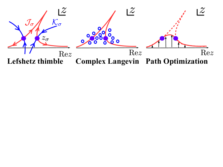
Figure 1: Schematic picture of integration path and sampled configurations in the Lefschetz thimble method (left), the complex Langevin method (middle), and the path optimization method (right).

As in the above case, if we can choose the integral path going through the saddle point dominantly contributing to the integral, we can avoid the integral of rapidly oscillating function and we can avoid the sign problem. This is a basic idea used in the method using the integral over complexified variables. In the Lefschetz thimble method (LTM) [23, 24, 25, 26], the integral path (manifold) $J_{\sigma}$, referred to as the thimble(s), is obtained by solving the flow equation, $\dot{z}_{i}=\overline{\partial S/\partial z_{i}}$, from the fixed point $\sigma$ ($\left.\partial S/\partial z_{i}\right|_{\sigma}=0$), as shown in the left panel of Fig. 1. On the thimble, the imaginary part of the action is constant, and the sign problem is weakened. But we still have several problems in applying LTM to field theories. For example, the integral measure $d^{N}z$ contains the complex phase which is generally not constant (residual sign problem), and when two or more thimbles contribute to the partition function, the integrals on different thimbles can have different complex phases and would cancel each other (global sign problem). In addition, finding fixed points and constructing relevant thimbles are not easy. For the last point, a more practical method, referred to as the generalized Lefschetz thimble method (GLTM), to obtain relevant thimbles is proposed [26]. By evolving the integral path by using the flow equation from the real axis (original integration path), the path becomes closer to relevant thimbles. Even if we do not reach the thimble, the phase fluctuation is generally suppressed on the evolved path.

The complex Langevin method (CLM) [27, 28, 29, 30, 31, 32, 10, 11, 12, 13, 14] is another promising approach. By solving the complex Langevin equation, $\dot{z}_{i}=-\partial S/\partial z_{i}+\eta_{i}(t)$ with $\eta_{i}$ being the white noise, we can generate configurations around the fixed point as shown in the middle panel of Fig. 1, and we can calculate observables as an ensemble average, $\langle\mathcal{O}\rangle=\langle\mathcal{O}\rangle_{\mathrm{CLM}}$. Since no phase reweighting is necessary, there is no sign problem, in principle. Thanks to recent developments of the gauge cooling technique [31] and the deformation technique to avoid the singular point of the action [32], one can perform stable simulations even at high density region. One of the problems in the complex Langevin method is the occasional convergence to wrong results. When the magnitude distribution of the drift term has a long tail than the exponential decay, the results are not reliable even if they converge [30]. Unfortunately, the current CLM simulations are not reliable in the phase transition region at low temperatures [13]. We need further analyses to understanding the origin of the long tail.

In the last lattice meeting [33] and in Ref. [34], we have proposed another method, the path optimization method (POM), in which the integration path is optimized to evade the sign problem, i.e. to enhance the average phase factor. Since there is no singular point of the Boltzmann weight at finite $z$ in most of physical systems, the integral of the Boltzmann weight is independent of the path. (The exception is the lattice simulations with the Fermion determinant rooting, $\sqrt{\det D}\,\exp(-S_{G})$, which gives rise to the cut in the Boltzmann weight.) It should be noted that the zero point of the Fermion determinant is the singular point of $S_{\mathrm{eff}}$, but just a zero point of the Boltzmann weight $\exp(-S_{\mathrm{eff}})$. Then the optimization can be done in various ways. For example, using the flow equation is one of the ways to optimize the path as in GLTM. In one dimensional integral, we can parameterize the imaginary part by a trial function of the real part, and optimize the trial function by the standard gradient descent method [34]. It is also possible to utilize the neural network [35, 36]. Because of this flexibility, similar ideas have been applied to several problems recently: 1+1 dimensional $\phi^{4}$ theory [35], 0+1 dimensional $\phi^{4}$ theory [37], 2+1 dimensional finite density Thirring model (their method is referred to as the sign-optimized manifold method (SOMMe)) [16, 17], 1+1 dimensional QED [18], and the Polyakov-loop extended Nambu-Jona-Lasinio (PNJL) model [36].

When we have many variables as in the field theories, the neural network is a useful tool: It can describe any functions of many variables, then it is equivalent to prepare the complete set of trial functions. In this proceedings, we apply the path optimization method with use of the neural network to field theories with the sign problem. After a brief review of the path optimization method, the neural network, and the stochastic gradient method, we discuss 1+1 dimensional $\phi^{4}$ theory at finite $\mu$ [35], 0+1 dimensional QCD at finite $\mu$ [38], and the Polyakov-loop extended Nambu-Jona-Lasinio (PNJL) [36].

2 Path optimization with use of neural network

We consider the case where the Boltzmann weight $\exp(-S)$ is a complex and analytic function of the field variables $x=\{x_{i};i=1,2,\ldots N\},x_{i}\in\mathbb{R}$ with $N$ being the number of variables. By complexifying the field variables $z_{i}=x_{i}+iy_{i}$, the Boltzmann weight becomes a holomorphic (complex analytic) function of the complexified field variables $z$. The partition function can be written as

$$\mathcal{Z}=\int_{\mathcal{C}_{\mathbb{R}}}d^{N}x\,\exp(-S(x))=\int_{\mathcal{C}_{\mathbb{C}}}d^{N}z\,\exp(-S(z))=\int_{\mathcal{C}_{\mathbb{R}}}d^{N}x\,J(z)\exp(-S(z))\ ,$$ (2)

where $J(z)=\det(\partial z_{i}/\partial x_{j})=\det(\delta_{ij}+i\partial y_{i}/\partial x_{j})$ is a Jacobian. We here assume that the imaginary part of the complexified variables are given as functions of the real part, $y_{i}=y_{i}(x)$, which specify the integration path. If we can optimize the functions $y_{i}(x)$ to enhance the average phase factor to be clearly above zero, precise calculation of observables becomes possible.

In the path optimization method, we optimize the integration path specified by $y(x)=\{y_{i}(x);i=1,2,\ldots N\}$ to minimize the cost function, which represents the seriousness of the sign problem. We adopt the following cost function,

$$\mathcal{F}[y]=\mathcal{Z}_{\mathrm{pq}}-|\mathcal{Z}|=|\mathcal{Z}|\left(|\langle{e^{i\theta}}\rangle|^{-1}-1\right)\ ,$$ (3)

where $\theta$ is the complex phase of the statistical weight, $W=J(z)\exp(-S(z))$, and $\mathcal{Z}_{\mathrm{pq}}$ is the phase quenched partition function. Since the partition function is independent of the path, the above cost function is a monotonically decreasing function of the average phase factor.

Optimization of the path can be performed via the gradient descent method or by using the neural network which is used in machine learning. In the one-dimensional integral case, we can expand the imaginary part by a complete set of functions, $y(x)=\sum_{n}c_{n}H_{n}(x)$ with $\{H_{n}\}$ being a complete set, and tune the coefficients $c_{n}$ to minimize the cost function using the gradient descent method. In Ref. [34], we have found that the optimized path is close to the thimble around the fixed points. Thus the path optimization may be also regarded as a practical method to search for the thimble. On the optimized path, the rapid oscillation of the integrand is suppressed, while the absolute values becomes smaller. The hybrid Monte Carlo sampling works well on the optimized path, and it is possible to calculate the observables precisely.

When we have many integral variables as in the field theories, it is tedious and practically impossible to prepare the complete set of functions and to optimize the path. The number of expansion parameters is $M^{N}$, where $M$ is the number of functions for each degrees of freedom needed for conversion. We need to avoid the exponential growth of the number of parameters.

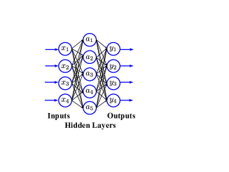
Figure 2: Schematic picture of the neural network.

One of the ways to avoid the above exponential growth is to utilize the feedforward neural network. The neural network is a mathematical model of the human brain. It contains the input, hidden, and output layers, and each layer consists of units which mimic neurons as schematically shown in Fig. 2. Units in one layer is connected with those in the previous and next layers, and the variables are modified by combining the linear and non-linear transformations. In the single hidden layer case, these transformations are given as

$$a_{i}=g(W^{(1)}_{ij}x_{j}+b^{(1)}_{i})\ ,\ \ y_{i}=\alpha_{i}(g(W^{(2)}_{ij}a_{j}+b^{(2)}_{i}))+\beta_{i}\ ,$$ (4)

where $g(x)$ is called the activation function and we adopt $g(x)=\tanh x$ in order to keep the differentiability. We input $\{x_{i}\}$ and obtain $\{y_{i}\}$ as the outputs. $W^{(1,2)}_{ij}$, $b^{(1,2)}_{i}$, $\alpha_{i}$ and $\beta_{i}$ are the parameters in the neural network. The number of parameters is $\mathcal{O}(N^{2})$ where $N$ is the number of variables, provided that the number of units in the hidden layer is proportional to $N$ and the number of layers is $\mathcal{O}(1)$. The universal approximation theorem [39] tells us that any functions can be described in the large number limit of the units in the hidden layers, even in the case of a single hidden layer.

In updating the parameters in the neural network, we apply the stochastic gradient method. We adopt the ADADELTA algorithm [40],

$$F_{i}^{(j)} =\partial\mathcal{F}/\partial c_{i}^{(j)}\ ,$$ (5)

$$r_{i}^{(j+1)} =\gamma r_{i}^{(j)}+(1-\gamma)(F_{i}^{(j)})^{2}\ ,$$ (6)

$$v_{i}^{(j+1)} =\frac{\sqrt{s_{i}^{(j)}+\epsilon}}{\sqrt{r_{i}^{(j+1)}+\epsilon}}F_{i}^{(j)}\ ,$$ (7)

$$c_{i}^{(j+1)} =c_{i}^{(j)}-\eta v_{i}^{(j+1)}\ ,$$ (8)

$$s_{i}^{(j+1)} =\gamma s_{i}^{(j)}+(1-\gamma)(v_{i}^{(j+1)})^{2}\ ,$$ (9)

where $c_{i}^{(j)}$ represents the $i$-th parameter in the $j$-th step of updates, and $\mathcal{F}$ is the cost function. Gradients $F_{i}^{(j)}$ are evaluated as the average in a small number ($N_{\mathrm{batch}}$) of configurations (mini-batch training), and their squared average is stored in $r_{i}^{(j)}$. The parameters are updated by using the ”velocity” $v_{i}^{(j)}$, gradients normalized by the root mean square in the history of updates. The squared averages of $v_{i}^{(j)}$ are stored in $s_{i}^{(j)}$. The learning rate $\eta$ plays the role of the time step, and $\gamma$ is referred to as the decay rate in machine learning but is the survival rate in the actual meaning. When the derivative and velocity become smaller than the cutoff parameter $\epsilon$ during many updates, the ADADELTA algorithm becomes equivalent to the standard gradient descent method, $\dot{c}_{i}=-\partial\mathcal{F}/\partial c_{i}$.

Usually, the neural network is trained by using the teacher data, where the answers are prepared (supervised learning). By comparison, we do not know the optimized path in advance, then the parameters in the neural network are updated only by the gradient of the cost function. This update corresponds to the so-called unsupervised learning.

We generate the Monte Carlo configurations by the hybrid Monte Carlo (HMC). We regard the real part of variables as the dynamical variable, where the molecular dynamics Hamiltonian is $H(x,p)=p^{2}/2+\mathrm{Re}S(z(x))$. The derivative of the Jacobian requires numerical cost and is ignored in the molecular dynamics evolution. We solve the canonical equation of motion, $\dot{x}=p$ and $\dot{p}=-\partial H/\partial x$, and make Metropolis judgement with the Jacobian effects included. We prepare $N_{\mathrm{config}}$ configurations, update parameters using $N_{\mathrm{batch}}$ configurations in each mini-batch training. After updating parameters $N_{\mathrm{config}}/N_{\mathrm{batch}}$ times, we generate $N_{\mathrm{config}}$ configurations using the updated neural network parameters. We repeat this update process $N_{\mathrm{epoch}}$ times. One epoch means the number of updates where the $N_{\mathrm{config}}$ configurations are used in the mini-batch training.

The path optimization with use of the neural network has been applied to the one-dimensional integral [33]. The obtained optimized path is close to the thimble and the path optimized by using the standard gradient descent method around the fixed points. These paths do not agree off the fixed points. The statistical weights are small far off the fixed points, and do not contribute to the observable calculation much.

3 Application to field theory: complex $\phi^{4}$ theory

Now let us apply the path optimization method with use of the neural network to the 1+1 dimensional complex $\phi^{4}$ theory at finite $\mu$. The Lagrangian of the complex $\phi^{4}$ theory is given as $\mathcal{L}=\partial_{\mu}\phi^{*}\partial^{\mu}\phi-m^{2}\phi^{*}\phi-\lambda(\phi^{*}\phi)^{2}$, and the action at finite $\mu$ on the Euclidean lattice is given as

$$S=\sum_{x} \left[\frac{(4+m^{2})}{2}\phi_{a,x}\phi_{a,x}+\frac{\lambda}{4}(\phi_{a,x}\phi_{a,x})^{2}-\phi_{a,x}\phi_{a,x+\hat{1}}-\cosh\mu\,\phi_{a,x}\phi_{a,x+\hat{0}}+i\epsilon_{ab}\sinh\mu\,\phi_{a,x}\phi_{b,x+\hat{0}}\right]\ ,$$ (10)

where $\phi=(\phi_{1}+i\phi_{2})/\sqrt{2}$ with $\phi_{a}(a=1,2)$ being the real scalar field. The last term of the action gives rise to the imaginary part, and we have the sign problem. We complexify the real and imaginary parts, $\phi_{1,x}=\varphi_{1,x}+i\xi_{1,x}$ and $\phi_{2,x}=\varphi_{2,x}+i\xi_{2,x}$, respectively, and apply the path optimization method.

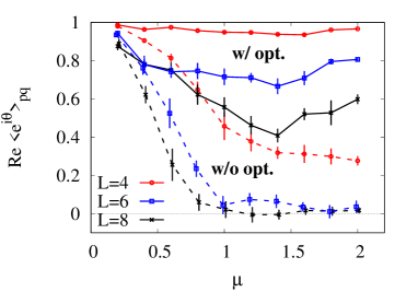
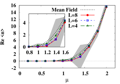
Figure 3: Average phase factor (left) and number density (right) in the complex $\phi^{4}$ theory at finite $\mu$.

We have performed the optimization of the integration path on $4^{2},6^{2}$ and $8^{2}$ lattices with $m=\lambda=1$ by using the neural network with a single hidden layer. In the left panel of Fig. 3, we show the average phase factor as a function of $\mu$. Without the optimization, the average phase factor quickly decreases towards zero. By comparison, the HMC simulation on the optimized path shows that the average phase factor is enhanced and kept to be greater than 0.4. Then the statistical error of the expectation value for a given number of configurations is much smaller on the optimized path (lines) than that on the original path (gray area) as shown in the right panel of Fig. 3. The calculated number density, $n=-\partial(S/V)/\partial\mu$, starts to grow at around $\mu=1$, as expected from the mean field results, $\mu_{c}(\mathrm{MF})=\mathrm{arccosh}\,(1+m^{2}/2)\simeq 0.96$, while the growth is delayed compared with the mean field results especially on the larger lattices.

These features qualitatively agree with the results in previous works [25, 41], where 3+1 dimensional complex $\phi^{4}$ theory is discussed using CLM [41] and LTM [25]. It is found that the rapid decay of the average phase factor on the original path or in the phase quenched simulations, enhanced average phase factor on the thimble [25], and delay of the density growth due to the interaction.

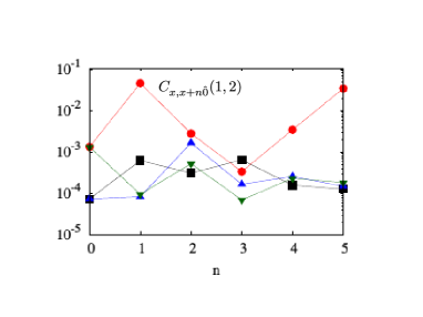
Figure 4: Correlation between the imaginary and real parts, $C_{xy}(a,b)$, on a $6^{2}$ lattice.

The average phase factor may not be large enough compared with the LTM results [25]. This should be due to incomplete optimization. Good ansatz helps us to enhance the average phase factor. For example, Bursa and Kroyter have proposed several ansatz in the 0+1 dimensional complex $\phi^{4}$ theory using the translational invariance and the $\mathrm{U}(1)$ symmetry [37]. By using their ansatz, the average phase factor is well above 0.9 at $L=8$ with $L$ being the temporal lattice size. The ansatz in Ref. [37] assumes that the imaginary part of the variable on a site is a function of the real part on the same and the nearest neighbor sites. Also in our calculation, the correlation $C_{xy}(a,b)=(\partial\xi_{a,x}/\partial\varphi_{b,y})^{2}+(\partial\xi_{b,y}/\partial\varphi_{a,x})^{2}$ is found to be strong for the nearest neighbor sites in the temporal direction, $x$ and $x+\hat{0}$, as shown in Fig. 4, and other correlations are smaller by about 2 orders of magnitude. Thus assuming the dependence $\xi_{a,x}=f_{a}(\varphi_{x},\varphi_{x\pm\hat{0}})$ would be a good starting point of unsupervised learning.

4 Application to gauge theory: 0+1 dimensional QCD

As the first step of application to gauge theory, we discuss 0+1 dimensional QCD with one species of staggered Fermion at finite $\mu$ on a $1\times N_{\tau}$ lattice [42, 43, 44, 45, 46, 47]. The lattice action is given as

$$S= \frac{1}{2}\!\sum_{\tau}\left(\bar{\chi}_{\tau}e^{\mu}U_{\tau}\chi_{\tau+\hat{0}}\!-\!\bar{\chi}_{\tau+\hat{0}}e^{-\mu}U^{-1}_{\tau}\chi_{\tau}\right)\!+\!m\sum_{\tau}\!\bar{\chi}_{\tau}\chi_{\tau}=\frac{1}{2}\bar{\chi}D\chi\ .$$ (11)

The partition function is obtained as

$$\mathcal{Z}= \int\mathcal{D}U\det{D[U]}=\int dU\det\left[X_{N_{\tau}}\!+\!(-1)^{N_{\tau}}e^{\mu/T}U+\!e^{-\mu/T}U^{-1}\right]$$

$$= \frac{\sinh[(N_{c}+1)E/T]}{\sinh[E/T]}+2\cosh(N_{c}\mu/T)\ ,$$ (12)

$$X_{N_{\tau}}= 2\cosh(E/T)\ ,\ E=\mathrm{arcsinh}\,m\ ,\ U=U_{1}U_{2}\cdots U_{N_{\tau}}\ ,\ T=1/N_{\tau}\ .$$ (13)

It should be noted that only the product of link variables, $U=U_{1}U_{2}\cdots U_{N_{\tau}}$, remains in the partition function, then 0+1 dimensional QCD reduces to a one link problem.

The 0+1 dimensional QCD is a toy model, but it contains the temporal hopping term which is the actual source of the sign problem in 3+1 dimensional QCD. The properties of the above partition function is also studied well in the context of the strong coupling lattice QCD [48, 49].

By using the residual gauge degrees of freedom, it is also possible to take the diagonal gauge. The link variable for color $\mathrm{SU}(3)$ in the diagonal gauge is given as $U=\mathrm{diag}(e^{ix_{1}},e^{ix_{2}},e^{ix_{3}})$ with $x_{1}+x_{2}+x_{3}=0$. After complexification of gauge variables, the partition function is now given as

$$\mathcal{Z}= \int dUe^{-S}=\int dx_{1}dx_{2}JHe^{-S}$$

$$= \int dx_{1}dx_{2}\left[\det\left(\frac{\partial z_{a}}{\partial x_{b}}\right)\right]\left[\frac{8}{3\pi^{2}}\prod_{a<b}\sin^{2}\left(\frac{z_{a}-z_{b}}{2}\right)\right]\left[\prod_{a}\left(X_{N_{\tau}}+2\cos(z_{a}-i\mu)\right)\right]\ ,$$ (14)

where the color index ($a,b$) runs from 1 to $N_{c}(=3)$, and $z_{1}=x_{1}+iy_{1},z_{2}=x_{2}+iy_{2}$ and $z_{3}=-(z_{1}+z_{2})$. The part in the first square bracket represents the Jacobian $J$, the second is the Haar measure $H$, and the third is the Boltzmann weight $\exp(-S)=\det D$. We have assumed that $N_{\tau}$ is an even number.

We have only two variables in the diagonal gauge, then it is possible to work on the two dimensional mesh points of $(x_{1},x_{2})$. We first discuss the results where the imaginary parts $(y_{1},y_{2})$ themselves are treated as the parameters. The gradient descent equation is then given as

$$\frac{dy_{i}(x_{1},x_{2})}{dt}=-\frac{\partial\mathcal{F}}{\partial y_{i}(x_{1},x_{2})}\ ,$$ (15)

where $t$ is the fictitious time.

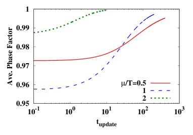
Figure 5: Average phase factor in 0+1 dimensional QCD.

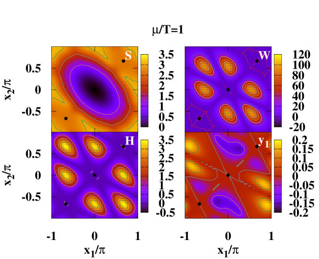
Figure 6: Action $S$ (from the minimum, left top), Haar measure $H$ (left bottom), the statistical weight $He^{-S}$, and the imaginary part of variable $y_{1}$ in 0+1 dimensional QCD.

We have performed path optimization for 0+1 dimensional QCD with $T=1/2$ and $m=0.05$. By optimizing the path, the average phase factor goes above 0.99 easily as shown in Fig. 5. It is partly because the average phase factor on the original path is above 0.95. Nevertheless we would like to emphasize that the reduction of $(1-\mathrm{APF})$ is significant. In the 3+1 dimensional calculation, the 0+1 dimensional QCD action appears in each spatial point on the lattice, then the average phase factor in 3+1 dimensions on a $L^{3}\times N_{\tau}$ lattice would be around the $L^{3}$-th power of that in the 0+1 dimensions, $\mathrm{APF}_{3+1}\simeq(\mathrm{APF}_{0+1})^{L^{3}}$, provided that other action terms do not make it worse. Then $\mathrm{APF}_{0+1}=0.95$ leads to $\mathrm{APF}_{3+1}\simeq 4\times 10^{-12}$ on a $8^{3}\times N_{\tau}$ lattice, while $\mathrm{APF}_{0+1}=0.995$ gives $\mathrm{APF}_{3+1}\simeq 0.08$. This average phase factor is not large but it would be enough to obtain some meaningful results.

The results of path optimization for $\mu/T=1$ is shown in the right-bottom panel of Fig. 6. The imaginary part $y_{1}$ is modified from zero (original path) to be in the range of $-0.2<y_{1}<0.2$ after optimization. ($y_{2}$ is obtained by exchanging $x_{1}$ and $x_{2}$ axes.) The amount of the shift is roughly proportional to $-\partial\mathcal{F}/\partial y_{i}$, as expected from perturbation. The action shows a deep minimum at $(x_{1},x_{2})=(0,0)$, and there are two local minima at $(x_{1},x_{2})=\pm(2\pi/3,2\pi/3)$. By comparison, the Haar measure divides the plain into the six separated regions. As a result, the probability distribution, the real part of $W=H\exp(-S(z))$ (except for the Jacobian), also has six regions.

The diagonal gauge is useful as shown above, but there are two problems. One is that it is not always possible to take this gauge for all links. When we have spatial dimensions, we can take the diagonal gauge for temporal links but not for spatial links. The other is the separated probability distribution. The separated distribution does not cause trouble in mesh point integral, but is problematic in HMC simulations. Since it is difficult to overcome the statistical barrier from the Haar measure, we need to invoke the exchange Monte Carlo or different tempering [50, 51] in order to sample configurations in the above six regions equally well.

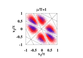
Figure 7: Distribution of $(x_{a},x_{b})$ ($a\not=b$) in HMC simulations in 0+1 dimensional QCD.

Now we proceed to link variable sampling without diagonal gauge fixing. The $\mathrm{SU}(3)$ link variable $U$ is complexified to a $\mathrm{SL}(3)$ variable $\mathcal{U}$. We here adopt the following complexification,

$$U\in\mathrm{SU}(3)\to\mathcal{U}(U)=U\,\prod_{a=1}^{N_{c}^{2}-1}e^{y_{a}\lambda_{a}/2}\in\mathrm{SL}(3)\ .$$ (16)

This form of the link variable is convenient to calculate the derivative of the matrix element with respect to the real part of variables as well as the imaginary part. Since we have eight variables, mesh point integral is not possible. We adopt HMC for sampling, and the neural network for optimization. In HMC, we regard the $\mathrm{SU}(3)$ part is regarded as the dynamical variable of the molecular dynamics, and the Hamiltonian is taken to be $H=P^{2}/2+\mathrm{Re}S(\mathcal{U}(U))$, where $P$ is the conjugate momentum matrix of $U$.

We have performed the path optimization using a neural network for the link variable without gauge fixing [38]. After optimization, we generate configurations in HMC using the optimized neural network. The $\mathrm{SL}(3)$ link variables can be diagonalized by the similarity transformation, $\mathcal{U}\to P^{-1}\mathcal{U}P$. The diagonalized link variables are given as $\mathrm{diag}(e^{iz_{1}},e^{iz_{2}},e^{iz_{3}})$ with $z_{1}+z_{2}+z_{3}=0$. In Fig. 7, we show the distribution of $(x_{a},x_{b})$ ($a\not=b$) with $x_{a}=\mathrm{Re}\,z_{a}(a=1,2,3)$. We show the distribution with $(a,b)=(1,2)$ with blue dots and other combinations of $(a,b)$ with red dots. This distribution (blue+red) is consistent with that in the probability distribution in the diagonalized gauge. While the order of the eigenvalues may be easily exchanged in the diagonalization, we can deduce that the six separated regions are visited in the HMC sampling. This is natural because the six regions are related with each other by the exchange $z_{a}\leftrightarrow z_{b}(a,b=1,2,3)$ and by the symmetry $S(-z)=(S(z^{*}))^{*}$ which corresponds to the transformation of $x_{a}\to-x_{a}$, and the the eight variable link variable contains these transformations.

We have also confirmed that we can reproduce the exact results of the chiral condensate, quark number density, and the Polyakov loop in both of the treatment of link variables within the statistical errors. These results will be reported in the forthcoming paper [38].

5 Application to QCD effective model with phase transition: PNJL model with homogeneous ansatz

One important task in tackling the sign problem is how to handle the multi thimble contributions. When we have two or more fixed points contributing to the partition function significantly, jumping from the one to other in HMC simulations requires more elaborate procedures. The separated regions of probability in the 0+1 dimensional QCD are apparent ones and are connected in the $\mathrm{SL}(3)$ link variables. By comparison, one expects the phase transition in dense QCD, where two different configurations of the chiral condensate and the Polyakov loop, hadronic and quark matter, compete at around the phase transition boundary. This would correspond to the two fixed point problem. In other words, two thimbles starting from these two fixed points would contribute significantly to the partition function.

As an example to discuss the phase transition, the Polyakov loop extended Nambu-Jona-Lasinio (PNJL) model [52] seems to be nice. In the mean field approximation, we find the first order phase transition boundary in low $T$ and finite $\mu$ region. When we take account of fluctuations of fields, the PNJL model has the sign problem. We have applied the path optimization method to the PNJL [36]. The Fourier transformed field variables are truncated at zero momentum, i.e. homogeneous field ansatz is used, while the volume is assumed to be finite. In this setup, the finite volume results should converge to the mean field results in the large volume limit.

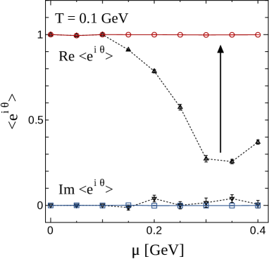
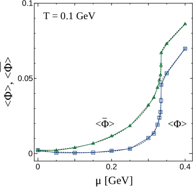
Figure 8: The average phase factor (left) and the Polyakov loop and its conjugate (right) in the PNJL model.

In Fig. 8, we show the results of path optimization of the PNJL model at $T=100\,\mathrm{MeV}$ and volume $k=64$ [36]. We take the the diagonal gauge, and $A_{3}$ and $A_{8}$ are complexified, while $\sigma$ and $\vec{\pi}$ are kept to be real. This choice corresponds to the complexification in the diagonalized gauge in the 0+1 dimensional QCD, discussed in the previous section. At around the transition chemical potential, $\mu\simeq 330\,\mathrm{MeV}$, the average phase factor is suppressed without optimization, while it becomes almost unity after optimization. The finite volume results converge to the mean field results with increasing volume. The phase transition signal, the rapid increase of the Polyakov loop ($\Phi$) and its conjugate ($\overline{\Phi}$), is described well on the optimized path as found in the right panel of Fig. 8.

6 Summary

The sign problem is a grand challenge in theoretical physics, and we encounter it in many subjects in physics. Recent development of complexified variable methods such as the Lefschetz thimble method, complex Langevin method, and the path optimization method encourages us to tackle the sign problem, while these methods may be still premature.

In this proceedings, we have discussed the sign problem in field theories by using the path optimization method with use of the neural network. In the path optimization method, we complexify integration variables as $x_{i}\to z_{i}=x_{i}+iy_{i}$. The integral path (manifold) is specified by the imaginary part as a function of the real parts $y_{i}(x)$, and is optimized to evade the sign problem. We can explicitly parameterize the imaginary part of variables, $y_{i}=y_{i}(\{x\})$, when the number of degrees of freedom is small. By comparison, it is not practical to prepare and optimize explicit functions by hand in the case with many variables such as in field theories. In such cases, the neural network used in machine learning is useful. We have adopted a neural network with a single hidden layer. It should be noted that even with a single hidden layer, the neural network can describe any functions in the large unit number limit. We have demonstrated the usefulness of the path optimization with use of the neural network in the complex $\phi^{4}$ theory at finite $\mu$ the 0+1 dimensional QCD at finite $\mu$, and the Polyakov loop extended Nambu-Jona-Lasinio model with homogeneous field ansatz. In all of these cases, the average phase factor is enhanced and the observables are obtained precisely.

One of the problems in the path optimization is the numerical cost. Since we aim to reduce the sum of complex phases from the Boltzmann weight $\exp(-S)$ and the measure or Jacobian $J(z)$ simultaneously, we need to calculate the Jacobian, where the numerical cost is $\mathcal{O}(N^{3})$ with $N$ being the number of variables. In order to reduce the cost, it is helpful to assume the function form of the imaginary part. For example, the imaginary part is assumed to be a function of the real part on the same lattice site in the Thirring model in Ref. [16], and it is assumed to be a function of the real part in the same and the nearest neighbor sites in 0+1 dimensional $\phi^{4}$ theory in Ref. [37]. These assumptions have been demonstrated to work well in enhancing the average phase factor. When the Jacobian matrix becomes sparse, we can save the numerical cost.

It is also interesting to apply the deep learning, where the number of hidden layers is larger than three. If the integration path is very complex as human brain with around 7 layers [53] cannot imagine, we may have to invoke deep learning to find the path.

This work is supported in part by the Grants-in-Aid for Scientific Research from JSPS (Nos. 15H03663, 16K05350, 18K03618), and by the Yukawa International Program for Quark-hadron Sciences (YIPQS).

References

- [1] P. de Forcrand, PoS LAT 2009 (2009) 010.
- [2] C. Ratti, Rept. Prog. Phys. 81 (2018) 084301; in this proceedings.
- [3] S. Sharma and S. Mukherjee, in this proceedings.
- [4] P. Steinbrecher [for the HotQCD Collaboration], arXiv:1807.05607 [hep-lat]; in this proceedings.
-
[5]
J. N. Guenther [for the WB Collaboration], in this proceedings;
S. Borsanyi et al, arXiv:1805.04445 [hep-lat]. - [6] J. Goswami, F. Karsch, C. Schmidt, A. Lahiri, in this proceedings.
-
[7]
W. Unger, D. Bollweg, M. Klegrewe, in this proceedings;
G. Gagliardi, J. Kim and W. Unger, EPJ Web Conf. 175 (2018) 07047. - [8] M. Klegrewe, W. Unger, in this proceedings.
- [9] K. Zambello, F. Di Renzo, in this proceedings.
- [10] D. K. Sinclair and J. B. Kogut, arXiv:1810.11880 [hep-lat] (in this proceedings).
- [11] S. Tsutsui, Y. Ito, H. Matsufuru, J. Nishimura, S. Shimasaki, A. Tsuchiya, in this proceedings.
- [12] F. Attanasio, B. Jäger, arXiv:1810.12973 [hep-lat] (in this proceedings).
- [13] Y. Ito, S. Tsutsui, J. Nishimura, H. Matsufuru, A. Tsuchiya, S. Shimasaki, in this proceedings.
-
[14]
A. Joseph, P. Basu, K. Jaswin, in this proceedings;
P. Basu, K. Jaswin, A. Joseph, Phys. Rev. D 98 (2018) 034501. - [15] J. Wosiek and B. Ruba, arXiv:1810.11519 [hep-lat] (in this proceedings).
-
[16]
S. Lawrence, A. Alexandru, P. F. Bedaque, H. Lamm, N. Warrington,
in this proceedings;
A. Alexandru, P. F. Bedaque, H. Lamm, S. Lawrence, Phys. Rev. D 97 (2018) 094510. - [17] N. Warrington, A. Alexandru, P. F. Bedaque, H. Lamm, S. Lawrence, in this proceedings.
- [18] H. Lamm, A. Alexandru, G. Başar, P. F. Bedaque, S. Lawrence, in this proceedings; A. Alexandru, G. Başar, P. F. Bedaque, H. Lamm, S. Lawrence, Phys. Rev. D 98 (2018) 034506.
- [19] S. Tsutsui and T. M. Doi, Phys. Rev. D 94 (2016) 074009.
-
[20]
M. Ogilvie and L. Medina, in this proceedings;
L. Medina and M. C. Ogilvie, arXiv:1712.02842 [hep-lat]. - [21] B. Jaeger and P. de Forcrand, in this proceedings.
- [22] Y. Mori, K. Kashiwa, A. Ohnishi, Phys. Lett. B 781 (2018) 688.
- [23] E. Witten, AMS/IP Stud. Adv. Math. 50 (2011) 347.
- [24] M. Cristoforetti et al. [AuroraScience Collaboration], Phys. Rev. D 86 (2012) 074506.
- [25] H. Fujii, D. Honda, M. Kato, Y. Kikukawa, S. Komatsu, T. Sano, JHEP 1310 (2013) 147.
- [26] A. Alexandru, G. Basar, P. F. Bedaque, G. W. Ridgway, N. C. Warrington, JHEP 1605 (2016) 053.
- [27] G. Parisi and Y. s. Wu, Sci. Sin. 24 (1981) 483.
- [28] J. R. Klauder, Acta Phys. Austriaca Suppl. 25 (1983) 251.
- [29] G. Aarts, E. Seiler, I. O. Stamatescu, Phys. Rev. D 81 (2010) 054508.
- [30] K. Nagata, J. Nishimura, S. Shimasaki, Phys. Rev. D 94 (2016) 114515.
- [31] E. Seiler, D. Sexty, I. O. Stamatescu, Phys. Lett. B 723 (2013) 213.
- [32] Y. Ito and J. Nishimura, JHEP 1612 (2016) 009.
- [33] A. Ohnishi, Y. Mori, K. Kashiwa, EPJ Web Conf. 175 (2018) 07043.
- [34] Y. Mori, K. Kashiwa, A. Ohnishi, Phys. Rev. D 96 (2017) 111501.
- [35] Y. Mori, K. Kashiwa, A. Ohnishi, PTEP 2018 (2018) 023B04.
- [36] K. Kashiwa, Y. Mori, A. Ohnishi, Phys. Rev. D, in press; arXiv:1805.08940 [hep-ph].
- [37] F. Bursa and M. Kroyter, arXiv:1805.04941 [hep-lat].
- [38] Y. Mori, K. Kashiwa, A. Ohnishi, work in progress.
-
[39]
G. Cybenko,
Mathematics of control, signals and systems (MCSS) 2 (1989) 303;
K. Hornik, M. Stinchcombe, H. White, Neural Networks 2 (1989) 359. - [40] M. D. Zeiler, arXiv:1212.5701.
- [41] G. Aarts, Phys. Rev. Lett. 102 (2009) 131601.
- [42] N. Bilic and K. Demeterfi, Phys. Lett. B 212 (1988) 83.
- [43] L. Ravagli and J. J. M. Verbaarschot, Phys. Rev. D 76 (2007) 054506.
- [44] G. Aarts and K. Splittorff, JHEP 1008 (2010) 017.
- [45] J. Bloch, J. Phys. Conf. Ser. 432 (2013) 012023.
- [46] C. Schmidt and F. Ziesché, PoS LATTICE 2016 (2017) 076.
- [47] F. Di Renzo, and G. Eruzzi, Phys. Rev. D 97 (2018) 014503.
- [48] K. Miura, T. Z. Nakano, A. Ohnishi, Prog. Theor. Phys. 122 (2009) 1045; K. Miura, T. Z. Nakano, A. Ohnishi, N. Kawamoto, Phys. Rev. D 80 (2009) 074034; T. Z. Nakano, K. Miura, A. Ohnishi, Phys. Rev. D 83 (2011) 016014; T. Ichihara, A. Ohnishi and T. Z. Nakano, PTEP 2014 (2014) 123D02; K. Miura, N. Kawamoto, T. Z. Nakano, A. Ohnishi, Phys. Rev. D 95 (2017) 114505.
- [49] P. de Forcrand, J. Langelage, O. Philipsen, W. Unger, Phys. Rev. Lett. 113 (2014) 152002.
- [50] M. Fukuma, N. Matsumoto, N. Umeda, JHEP 1712 (2017) 001.
- [51] A. Alexandru, G. Basar, P. F. Bedaque, N. C. Warrington, Phys. Rev. D 96 (2017) 034513.
- [52] K. Fukushima, Phys. Lett. B 591 (2004) 277; Phys. Rev. D 77 (2008) 114028 [Erratum: Phys. Rev. D 78 (2008) 039902].
- [53] J. Defelipe, Front. Neuroanat. 5 (2011) 29.