Magneto-Ferroelectric Interaction in Superlattices: Monte Carlo Study of Phase Transitions

Abstract

We study in this paper the phase transition in superlattices formed by alternate magnetic and ferroelectric layers, by the use of Monte Carlo simulation. We study effects of temperature, external magnetic and electric fields, magnetoelectric coupling at the interface on the phase transition. Magnetic layers in this work are modeled as thin films of simple cubic lattice with Heisenberg spins. Electrical polarizations of $\pm{1}$ are assigned at simple cubic lattice sites in the ferroelectric layers. The transition temperature, the layer magnetizations, the layer polarizations, the susceptibility, the internal energy, the interface magnetization and polarization are calculated. The layer magnetizations and polarizations as functions of temperature are shown for various coupling interactions and field values. Mean-field theory is also presented and compared to MC results.

I Introduction.

The study of phase transitions, surface effects and critical phenomena in superlattices or multilayered magnetic nanofilms has been rapidly developed during the last two decades (see reviews diep:hal-01084599 ; Diep201631 ; Prudnikov2015 ; Ramazanov2016 ; kamilov1999 ). Such high interest in this area was stimulated by the fact that superlattices of nanofilm and multiferroics possess a number of unique properties which have a broad area of applications in nanoelectronics, spintronics Diep201631 ; pyatakov ; PhysRevLett ; Iijima_1992 ; Oneill2000 ; PhysRevB.55.11218 ; ramesh and devices using the giant magnetoresistance phenomenon diep:hal-01084599 ; Prudnikov2015 ; PhysRevB.85.184413 .

With modern technologies it is possible to create superlattices and multilayer nanofilms as thin as a few atomic layers from the crystal structures with magnetic and ferroelectric orderings. These structures are able to manifest magnetoelectric effects which are known to be the result of interactions between magnetic and ferroelectric subsystems. It should be noted that the study of magnetoelectric effects in these systems draws a great fundamental interest for their special features, such as size dependence of magnetic and ferroelectric order parameters and other characteristics pyatakov ; PhysRevLett ; Kharrasov2016 ; PhysRevB.73.094434 . For example, it has been shown that the change from the bulk values for films of a few dozens of monolayers ($d\geq 10$ nm) to the two-dimensional values for films thinner than 4-6 monolayers ($d\leq(1-2)$ nm) Prudnikov2015 ; Kharrasov2016 .

In Ref. lamekhov2015, it was shown that in heterostructures with magnetic and ferroelectric materials, the magnetoelectric effect induced by an external electric field is observed at the interface layer. This effect is accompanied by the appearance of an antiferromagnetic phase at the interface as well as with the change in the critical temperature of the magnetic layer. This has been observed experimentally in $\mathop{\rm La}_{0.87}\mathop{\rm Sr}_{0.13}\mathop{\rm Mn}\mathop{\rm O}_{3}/\mathop{\rm Pb}\mathop{\rm Zr}_{0.52}\mathop{\rm Ti}_{0.48}\mathop{\rm O}_{3}$ PhysRevB.87.094416 at certain concentrations of manganite. In the work Ref. Ort2014, with Monte Carlo (MC) simulation for a two-layer film with the structure $\mathop{\rm La}\mathop{\rm Sr}\mathop{\rm Mn}\mathop{\rm O}/\mathop{\rm Pb}\mathop{\rm Zr}\mathop{\rm Ti}\mathop{\rm O}$, phase transitions have been investigated and the correctly describing model has been proposed. A multi-sublattice model has been introduced to explain magnetic properties of compounds $\mathop{\rm R}_{2}\mathop{\rm Fe}_{17},\mathop{\rm Ho}_{2}\mathop{\rm Fe}_{11}\mathop{\rm Ti}$ and $\mathop{\rm Tb}\mathop{\rm Mn}_{6}\mathop{\rm Sn}_{6}$ 0953-8984-14-27-310 ; PhysRevB.66.014437 ; PhysRevB.55.12408 .

On theoretical points of view, one of the most studied systems for the layered magnetic structure was concentrated on the magnetic properties of magnetic bilayer Diepbook2 . Wei Wang et al. WANG2017104 have studied a ferrimagnetic mixed spin (1/2, 1) Ising double layer superlattice: they have shown the effects of the exchange coupling and the layer thickness on the compensation behavior and magnetic properties of the system, by MC simulation. Some interesting phenomena have been found, such as various types of magnetization curves, originating from the competition between the exchange coupling and temperature. In Ref. Fer2016, the phase diagram and magnetic properties of the mixed spin (1, 3/2) Ising ferroelectric superlattices with alternate layers have been investigated by means of MC simulation. It should be noted that they also investigated superlattice of only two ferroelectric layers with antiferroelectric interfacial interaction between layers, within the transverse Ising model. They found a number of interesting phenomena, such as the existence of the compensation temperature or transverse field to compensate the specific ranges of exchange interactions.

Note that MC methods based on the Metropolis algorithm, as well as other algorithms have proven to be successful in describing physical properties of magnetic systems of different spatial dimensions. They revealed particular features of the phase transitions in these systems landau2014guide . In Refs. Prudnikov2015, , phu2009crossover, , phu2009critical, and PhysRevB.91.014436, numerical studies of size effects in critical properties of the Heisenberg multilayer films with MC methods were conducted. For films of varying thickness an anisotropy induced, for example, by the crystalline field of the substrate, was taken into account. The precise calculation of critical indices was carried, the values of which have clearly demonstrated the dimensional transition from two-dimensional to three-dimensional properties of the films with increasing number of layers.

In this paper the methodology for Heisenberg multilayer films simulations diep:hal-01084599 ; landau2014guide is used for the MC simulation and the calculation of magnetic properties of multiferroic superlattices. Although previous valuable theoretical, numerical and experimental studies have been done, more research is still needed to further understand the magnetic, ferroelectric and thermodynamic properties of the superlattice. Our investigation is motivated by the fact that superlattices with magnetic and ferroelectric materials present great opportunities of applications in spintronics.

In the present paper, we will thus study the effects of the magnetoelectric coupling and the external magnetic and electric fields on the magnetic properties of the multiferroic superlattice shown in Fig. 1.

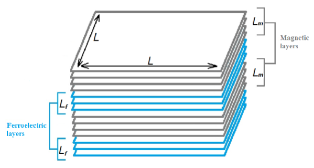
Figure 1: Schematic representation of the superlattice: alternate ferroelectric and magnetic films.

The paper is organized as follows. The model of the superlattice is presented in section II, where we summarize the principal steps used in the calculation of the ground-state configurations of the system. Section III shows the MC results of energy, layer magnetizations, susceptibilities and layer polarizations. Section IV shows results of another choice for interface coupling. The mean-field (MF) theory is shown in section V. Concluding remarks are given in section VI.

II Model and Ground State

II.1 Model

We consider a multilayer multiferroic films composed of $L_{z}^{m}$ ferromagnetic layers and $L_{z}^{f}$ ferroelectric layers alternately sandwiched in the $z$ direction (see Fig. 1). Each $xy$ plane has the dimension $L\times L$. The lattice sites of the magnetic layers of this superlattice are occupied by interacting Heisenberg spins $\vec{S}$, while the lattice sites of the ferroelectric layers are occupied by interacting polarizations $\vec{P}=\pm 1$ along the $z$ axis. Our system thus consists of a $L\times L\times L_{z}$ sites where $L_{z}=L_{z}^{m}+L_{z}^{f}$. We assume periodic boundary conditions in all directions to reduce surface effects. We assume interactions between ferroelectric and magnetic systems at their interfaces. The Hamiltonian of the system is defined as follows:

$${\cal H}=H_{m}+H_{f}+H_{mf},$$ (1)

The first term is the Hamiltonian of the magnetic subsystem, the second - of the ferroelectric subsystem, the third term is the Hamiltonian of their interaction. We assume

$$H_{m}=-\sum_{i,j}{J^{m}_{ij}\vec{S}_{i}\cdot\vec{S}_{j}}-\sum_{i}(\vec{H}\cdot\vec{S}_{i})$$ (2)

here $J^{m}_{ij}>0$ characterizes the ferromagnetic interaction between one spin and its nearest neighbors (NN). We consider it to be the same for NN within a layer and NN in adjacent layers. $\vec{S}_{i}$ is the classical Heisenberg spin occupying the i-th site. $\vec{H}$ is an applied magnetic field along the $+z$ direction. For the ferroelectric subsystem we write

$$H_{f}=-\sum_{i,j}{J^{f}_{ij}P_{i}\ P_{j}}-\sum_{i}{P}_{i}\ E^{z}$$ (3)

where $P_{i}$ is the polarization along the $z$ axis at the i-th site assumed to have only two values $\pm 1$ (Ising-like model), $J^{f}_{ij}>0$ denotes the NN ferroelectric interaction, similar for all NN. $E^{z}>0$ is the external electric field applied along the $+z$ axis perpendicular to the plane of the layers.

The magnetic interface layer creates at a site $k$ of the ferroelectric interface an effective field $H(k)$ along $z$ axis which is

$$H(k)=-J_{mf1}\sum_{i,j}{\vec{S}_{i}\cdot\vec{S}_{j}}-J_{mf2}\sum_{i,j}{\vec{S}_{i}\cdot\vec{S}_{j}},$$ (4)

so that the energy of interface magnetoelectric interaction of the polarization at the site $k$ can be written as

$$H_{mf}(k)=H(k)\ P_{k},$$ (5)

In this expression $J_{mf1}$ is the interaction parameter between the electric polarization component $P_{k}$ at the interface ferroelectric layer and its NN spin on the adjacent magnetic layer. $J_{mf2}$ is the interaction parameter between the electric polarization component $P_{k}$ at the interface ferroelectric layer and the next NN spin on the adjacent magnetic layer. These interactions are shown schematically in the Fig. 4.

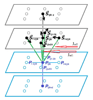
Figure 2: Schematic representation of magnetoelectric interactions at the interface between magnetic and ferroelectric layers.

Note that the interface coupling described by Eq. (5) is a scalar spin field acting on an electric polarization. Later, in section IV we will suppose another form for the coupling: a scalar polarization field acting on the $z$ spin component.

II.2 Ground state

Let us take positive $J^{m}_{ij}$ and $J^{f}_{ij}$ so that magnetic layers are ferromagnetic and ferroelectric layers have parallel polarizations, in the ground state.

The relative orientation between two adjacent magnetic and ferroelectric layers depends on the signs of $J_{mf1}$ and $J_{mf2}$. There are two simple cases:

i) if they are both positive, then spins and polarizations are parallel in the ground state (GS)

ii) if they are negative, then spins are antiparallel to polarizations in the GS.

The complicated case occurs when $J_{mf1}$ and $J_{mf2}$ have opposite signs. In this case, there is a competition between them which gives rise to some degree of frustration. For example, when $J_{mf1}>0$ and $J_{mf2}<0$ we have the situation where NN interaction wants $\vec{S}$ and $\vec{P}$ to be parallel, while the NNN interaction wants them to be antiparallel. Depending on their respective amplitudes, one configuration wins over the others.

Let us write the GS energy of a spin at the interface in zero fields

$$E_{1}=-Z_{1}J^{m}-Z_{2}J_{mf1}-Z_{3}J_{mf2}$$ (6)

where the coordination numbers are $Z_{1}=4,Z_{2}=1,Z_{3}=4$ for a simple cubic lattice.

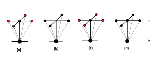
Figure 3: Ground state spin configurations with energies from $E_{1}$ to $E_{4}$ (a to d, respectively) depending on the interface interactions between magnetic and ferroelectric layers. Lower black circles are $P=1$ (up), upper black circles are up spins, red circles are down spins.

For $J_{mf1}<0$, the four spin configurations (see Fig. 3)

$$E_{1} = -Z_{1}J^{m}-Z_{2}|J_{mf1}|-Z_{3}|J_{mf2}|$$ (7)

$$E_{2} = -Z_{1}J^{m}+Z_{2}|J_{mf1}|-Z_{3}J_{mf2}$$ (8)

$$E_{3} = -Z_{1}J^{m}-Z_{2}|J_{mf1}|+Z_{3}J_{mf2}$$ (9)

$$E_{4} = +Z_{1}J^{m}-Z_{2}|J_{mf1}|-Z_{3}J_{mf2}$$ (10)

where $E_{1}$ is the energy of the state where all spins are down, all polarizations are up with $J_{mf2}<0$ (Fig. 3a). Other energies correspond to the spin configurations shown in Fig. 3: $E_{2}$ to Fig. 3b with $J_{mf2}>0$, $E_{3}$ to Fig. 3c with $J_{mf2}>0$ and $E_{4}$ to Fig. 3d with $J_{mf2}>0$.

The system will choose the GS depending on the values of $J_{mf1}$ and $J_{mf2}$. For simplicity, let us confine ourselves to GS configurations where all magnetic spins are parallel and all polarizations are parallel, i. e. the first three configurations. This choice is possible if the intralayer interactions $J^{m}>0$ and $J^{f}>0$ are sufficiently strong.

The state $E_{1}$ is chosen if

$$E_{1}<E_{2},E_{1}<E_{3},E_{1}<E_{4}$$ (11)

Solving these inequalities we have

$$J_{mf2}<0,|J_{mf1}|<\frac{Z_{1}J^{m}-Z_{3}J_{mf2}}{Z_{2}},|J_{mf1}|>0$$ (12)

namely,

$$J_{mf2}<0,|J_{mf1}|<4(J^{m}-J_{mf2}),J_{mf1}<0$$ (13)

Now we suppose $J_{mf2}>0$ then the GS will change to $E_{2}$. The critical value of $J_{mf2}$ and $J_{mf1}$ are determined by solving

$$E_{2}<E_{1},E_{2}<E_{3},E_{2}<E_{4}$$ (14)

We have

$$J_{mf2}>0,J_{mf1}<\frac{Z_{3}J^{mf2}}{Z_{2}},|J_{mf1}|<\frac{Z_{1}J^{m}}{Z_{2}}$$ (15)

namely,

$$J_{mf2}>1/4|J_{mf1}|,J_{mf2}>0,|J_{mf1}|<4J_{m}$$ (16)

The GS is $E_{3}$ if we have

$$E_{3}<E_{1},E_{3}<E_{4},E_{3}<E_{2}$$ (17)

We get

$$|J_{mf1}|>0,J_{mf2}<\frac{Z_{2}|J_{mf1}|}{Z_{3}},J_{mf2}<\frac{Z_{1}J^{m}}{Z_{3}}$$ (18)

or

$$J_{mf2}<1/4|J_{mf1}|,J_{mf2}<J^{m},|J_{mf1}|>0$$ (19)

In MC simulations shown below, care should be taken to choose the right GS according to values and signs of the interface interactions to avoid metastable states at low temperatures ($T$).

Note that we have taken $J_{mf1}<0$ in the above spin configurations. This is intended to have spins antiparallel to the magnetic field applied in the $+z$ direction so as to have a phase transition at a temperature with a finite field.

III Monte Carlo Simulation

For MC simulations we use the Metropolis algorithm and a sample size $L\times L\times L_{z}$ with $L=40,60,80,100$ for detection of lateral size effects and $L_{z}=8,16,12,24$ for thickness effects. When we investigate the effects of the magnetoelectric coupling on the magnetic, ferroelectric and interface properties, for simplicity we take the same size and thickness for the ferroelectric and magnetic layers (for example if $L_{z}=8$ - it means $L_{z}^{m}=4$ magnetic layers and $L_{z}^{f}=4$ ferroelectric layers). Exchange parameters between intralayer spins and intralayer polarizations are taken to be $J^{m}=J^{f}=1$ for the simulation.

For MC simulation we perform the cooling from the disordered phase: electrical polarizations of $\pm{1}$ are randomly assigned at lattice sites in the ferroelectric layers, in the $z$ direction. In the ferromagnetic layers spins with $|\vec{S}|=1$ are also randomly assigned in any direction, following in the spatial uniform distribution. At each $T$, new random $\vec{S_{i}}$ and $P_{i}$ were chosen, and the energy difference caused by this change is calculated. This change is accepted or rejected according to the Metropolis algorithm. In order to ensure the convergence of the observables, the lattice is swept 100000 times, where each time is considered as one MC step (MCS) that can be taken as the time scale of simulations. The observables of interest such as the averages of layer electric polarizations $P$, and layer magnetization $M$, are calculated over the following 50000 MCS. These quantities are defined as

$$P(n)=\frac{1}{L^{2}}\langle{|\sum_{i\in n}P_{i}|}\rangle$$ (20)

$$M(m)=\frac{1}{L^{2}}\langle{|\sum_{j\in m}\vec{S}_{j}}|\rangle$$ (21)

where $\langle...\rangle$ is the time average, and the sums on $i$ and $j$ are performed over the lattice sites belonging to the ferroelectric layer $n$ and the lattice sites belonging to the magnetic layer $m$, respectively. The process is repeated for a lower $T$ down to the desirable lowest one. We also perform the heating, starting from the GS spin configuration.

III.1 Zero fields

Monte Carlo results for energy, magnetization and polarization and their susceptibilities obtained by heating the system from the initial spin configuration of GS energy $E_{1}$ are shown in Fig. 4. Of course, starting from different initial spin configurations which are not the GS will lead to the same thermodynamic equilibrium but the equilibrating time is longer in particular at low $T$.

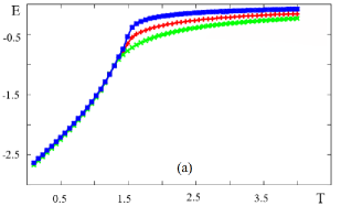
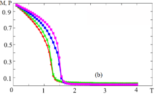
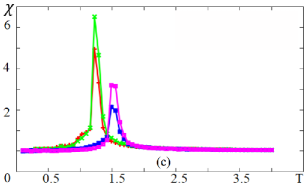
Figure 4: (a) Energy versus $T$. Red line: energy for total superlattice, green line: energy of magnetic layers, blue line: energy of ferroelectric layers ; (b) Magnetization and polarization versus $T$. Red line: magnetization of interface magnetic layers, green line: magnetization of interior magnetic layers, blue line: polarization of interface ferroelectric layers, purple line: polarization of interface ferroelectric layers ; (c) Susceptibilities versus $T$, with the same color code. $J^{m}=1,J_{mf1}=-0.15,J_{mf2}=-0.135$ corresponding to the GS with energy $E_{1}$.

MC results for energy, magnetization and polarization and their susceptibilities obtained by heating the initial spin configurations of energy $E_{2}$ are shown in Fig. 5. For $E_{3}$, the results are qualitatively similar (not shown). respectively.

The above figures show that the energy and other physical quantities well behave at low $T$ (no metastability) if we choose the correct GS according to the interface interaction. Note that the ferroelectric films undergo a phase transition at a temperature higher than that of the magnetic films. This is due to the Ising-like nature of the ferroelectric polarizations (in the bulk, the transition temperature is inversely proportional to $N$, the spin components, $\sim 1/N$). Also, the interface layers have lightly smaller order parameter than those inside the films.

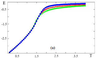
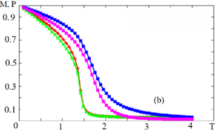
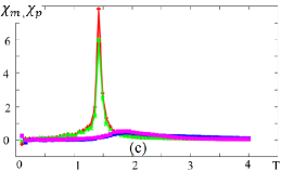
Figure 5: (a) Energy versus $T$. Red line: energy for total superlattice, green line: energy of magnetic layers, blue line: energy of ferroelectric layers ; (b) Magnetization and polarization versus $T$. Red line: magnetization of interface magnetic layers, green line: magnetization of interior magnetic layers, blue line: polarization of interface ferroelectric layers, purple line: polarization of interface ferroelectric layers ; (c) Susceptibilities versus $T$, with the same color code. $J^{m}=1,J_{mf1}=-0.15,J_{mf2}=0.8$ corresponding to the GS with energy $E_{2}$.

III.2 Particular Case $J_{mf1}=J_{mf2}$

In this section we present the results of the MC simulations in the particular case where $J_{mf1}=J_{mf2}$. We will compare these results with results from the MF theory.

Results for the temperature dependence of layer magnetizations, polarizations, and susceptibilities of the system are shown in Fig. 6 for $J_{m}=J_{f}=1,J_{mf}=J_{mf1}=J_{mf2}=-0.15,-0.55$. For $J_{mf}$, these curves present a sharp second-order transitions at $T_{c}^{m}\simeq 1.32$ for magnetic layers and $T_{c}^{f}\simeq 1.84$ for ferroelectric layers.

The results with an external magnetic field $H^{z}=0.7$ are shown in Fig. 7 for the order parameters. We can see that in this case the magnetic subsystem does not undergo a phase transition as a ferromagnet in a field. On the contrary, there is a second-order transition for ferroelectric layers at $T_{c}\simeq 1.84$.

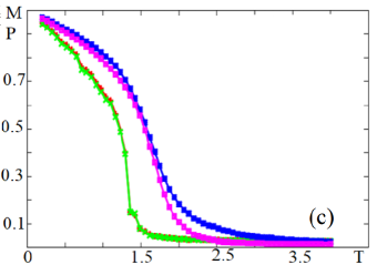
Figure 6: (a) Temperature dependence of layer magnetizations and layer polarizations, (b) layer susceptibilities, in the case $J^{m}=1$, $J^{f}=1$, $J_{mf}=-0.15$, $H^{z}=E^{z}=0$, $L=40$, $L_{z}=8$. Blue squares for the first layer and fourth magnetic layers (interface layers), black circles for the second and third (interior magnetic layers), magenta squares for the first and fourth (interface) ferroelectric layers, red for the second and third interior ferroelectric layers, respectively. $J_{mf1}=J_{mf2}$; (c) Temperature dependence of layer magnetizations and polarizations for $J^{m}=1$, $J^{f}=1$, $J_{mf}=-0.55$, $H^{z}=E^{z}=0$, $|\vec{S}|=1$, $P=\pm 1$. The coupling used is Eq. (24). Red and green lines are for magnetic interface and inner layers, magenta (blue) line for the interface (inner) ferroelectric layer.

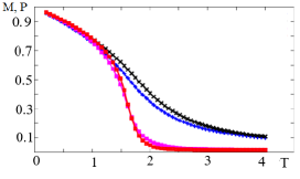
Figure 7: Temperature dependence of layer magnetizations and layer polarizations in case $J^{m}=1$, $J^{f}=1$, $J_{mf}(=J_{mf1}=J_{mf2})=-0.15$, $H^{z}=0.7$ and $E^{z}=0$, $L=40$, $L_{z}=8$. Blue squares for the first layer and fourth magnetic layers (interface layers), black circles for the second and third (interior magnetic layers), magenta squares for the first and fourth (interface) ferroelectric layers, red for the second and third interior ferroelectric layers, respectively.

With increasing $J_{mf}$, the system undergoes a first-order transitions. Fig. 8 shows the total magnetization $M$ and susceptibility versus $T$ for several values of $J_{mf}$ in the cross-over region from second to first order. The second-order phase transitions starts at $J_{mf}=0$ with $T_{c}\approx 2.456$, it decreases as $J_{mf}$ increases.

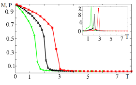
Figure 8: Temperature dependence of the total magnetization and susceptibility in case $J^{m}=1$, $J^{f}=1$, $J_{mf}=-1,-3,-5.5$, $H^{z}=E^{z}=0$, $L=40$, $L_{z}=8$. Red lines for $J_{mf}=-5.5$, black lines for $J_{mf}=-3$, green lines for $J_{mf}=-1$.

We show in Fig. 9 the case of $J_{mf}=-9.5$ where one can observe a discontinuity at the transition temperature $T_{c}\simeq 3.45$ for the interface magnetic layer and $T_{c}\simeq 3.49$ for the interface ferroelectric layer. Only layer $1$ and $4$ for magnetic and ferroelectric systems have a phase transition. Their order parameters strongly fall down at the transition temperature. This result is confirmed by several independent simulations. We calculate the transition temperature as a function of $J_{mf}$. We keep $J_{mf}$ constant, change the temperature and we take the transition temperature at the peak of the magnetic and ferroelectric susceptibility $\chi$. Note that for the strong interface coupling $J_{mf}=-9.5$, the interface order (black and blue curves in Fig. 9b) is so strong that it acts on the interior layer as an external field which does not allow the interior layer order parameter to go to zero: as a consequence, the interior layer undergoes only a smooth change of curvature at $T\simeq 1.5$ and falls to zero with the interface magnetic layer at $T_{c}\simeq 3.45$ (see red curve in Fig. 9b).

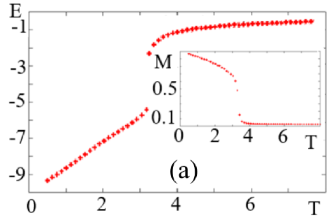
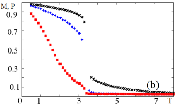
Figure 9: (a) Energy, layer magnetization (inset) versus $T$ ; (b) Interface layer magnetization (blue +), interior layer magnetization (red squares), interface polarization (black X) and interior layer polarization (magenta X overlapped under red squares), versus $T$. $J^{m}=1$, $J^{f}=1$, $J_{mf}=-9.5$, $H^{z}=E^{z}=0$ $L=40$, $L_{z}=8$.

Figure 10: Phase diagram in $T-J_{mf}$ plane. Here $J^{m}=1$, $J^{f}=1$, $H^{z}=E^{z}=0$.

The results for the transition temperature $T_{c}$ are shown in Fig. 10 as a function of $J_{mf}$. One can see that the transition temperature increases when we increase the values of $|J_{mf}|$. $T_{c}$ has a maximum at $J_{mf}=-8.5$. The second-order phase transition starts at $J_{mf}=0$ and becomes a first-order phase transition below $J_{mf}=-9$ (see Fig. 9 for $J_{mf}=-9.5$).

IV Another model of interface interaction

Let us show some results for the another model of magnetoelectric interaction given in the form

$$H^{1}_{mf}=-J_{mf}\sum_{i,j,k}P_{i}P_{j}S_{i}^{z}$$ (22)

We show in Fig. 12 layer magnetizations and polarizations as functions of interface coupling $J_{mf}$ For small values of the magnetoelectric interaction, magnetic and ferroelectric layers undergo phase transitions of different orders: magnetic layers undergo a phase transition of the first order, while ferroelectric layers undergo a the second-order transition, at temperatures $T_{c}\approx 0.63$ and $T_{c}\approx 1.52$, respectively.

With an increase of the magnetoelectric interaction $J_{mf}$ between the magnetic and ferroelectric subsystems, an unusual phenomenon is observed: the interface layers after $J_{mf}=-3.5$ undergo phase transitions of the first order. Note that in the model considered at the beginning of this article this occurs at large values of $J_{mf}=-9.5$. This is shown in Fig. 12a for the magnetic subsystem and in the inset for the ferroelectric layers.

For the inner layers of the magnetic subsystem, as the parameter $J_{mf}$ increases, the type of transition changes (Fig. 12b).

Phase diagram in Fig. 13a shows the effect of $J_{mf}$ on the transition temperature of the interface magnetic and ferroelectric layers. One can see that the transition temperature increases as the absolute value of $J_{mf}$ increases. At $J_{mf}=-3$ and below the transition temperatures for the magnetic and ferroelectric layers become distinct.

Phase diagram in Fig. 13b shows the effect of the external electric field $E$ on the transition temperature of the interface magnetic and ferroelectric layers. One finds that the transition temperature is almost unchanged when we increase $E^{z}$ up to $E^{z}=0.5$. For large values of $|J_{mf}|$ ($J_{mf}{\ll}-3$) the transition temperature is not sensitive to $E^{z}$.

Figure  11 shows the effect of the competition between the magnetoelectric interaction and the external electric field. With moderate magnetoelectric interaction ($J_{mf}=-2.5$), we can remark that the interface ferroelectric layer undergoes a second-order phase transition at $T_{c}=1.77$, the magnetic layers undergo a second-order phase transition at $T_{c}=1.64$. When we include an external electric field, both subsystems undergo a first-order phase transition at the same temperature $T_{c}=1.5$.

If the magnetoelectric interaction has a large value and the external electric field is zero, we have seen above that the interface magnetic and ferroelectric layers undergo a first-order phase transition. The inner magnetic layer undergoes a second-order phase transition while the internal ferroelectric layers are not subject to a phase transition. Now if we apply an electric field for instance $E^{z}=0.5$, the inner ferroelectric layers undergo a second-order phase transition (not shown).

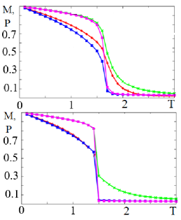
Figure 11: Temperature dependence of layer magnetizations and polarizations for $J^{m}=1$, $J^{f}=1$, $J_{mf}=-2.5$, $H^{z}=0$, with $E^{z}=0$ (top) and $E^{z}=0.5$ (bottom). The coupling is given by $H^{1}_{mf}$ (Eq. 22). Color code: magenta (or purple) lines for the first layer and fourth magnetic layers (interface layers), blue lines for the second and third (interior magnetic) layers. Green lines for the first and fourth (interface) ferroelectric layers, red lines for the second and third interior ferroelectric layers, respectively.

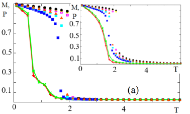
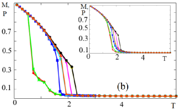
Figure 12: (a) Temperature dependence of interface layers of magnetic and ferroelectric films (inset) for $J^{m}=1$, $J^{f}=1$, $H^{z}=E^{z}=0$. Red line for the case $J_{mf}=-0.25$, green line for $J_{mf}=-0.5$. Blue points: $J_{mf}=-2.5$, light blue points: $J_{mf}=-3.5$, black points: $J_{mf}=-7$; (b) Temperature dependence of interior layers of magnetic and ferroelectric films (inset) with the same parameters and color code. The coupling is given by $H^{1}_{mf}$.

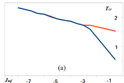
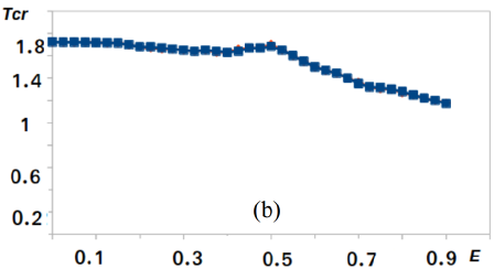
Figure 13: (a) Phase diagram in $T-J_{mf}$ plane. Here $J^{m}=1$, $J^{f}=1$, $H^{z}=E^{z}=0$. Red line and black line are for the ferroelectric critical temperature and the magnetic critical temperature, respectively. The coupling is given by $H^{1}_{mf}$ ; (b) Phase diagram in $T-E$ plane ($E$ stands for $E^{z}$). Here $J^{m}=1$, $J^{f}=1$, $H^{z}=0$, $J_{mf}=-3.5$.

To conclude this section, let us emphasize that beyond the two models for interface coupling studied above, the Dzyaloshinskii-Moriya interface interaction of the form $J_{mf}\vec{P}_{k}\cdot(\vec{S}_{i}\times\vec{S}_{j})$ may induce unexpected phenomena at the magneto-ferroelectric interface sergienko2006role ; diep2018skyrmion . Work is under way to investigate this coupling model.

V Mean-Field Theory

Let us show some analytical results obtained by us using the mean-field (MF) theory for the Hamiltonian

$${\cal H}=H_{m}+H_{f}+H_{mf},$$ (23)

where

$$H_{mf}=-J_{mf}\sum_{i,j,k}{\vec{S}_{i}\cdot\vec{S}_{j}}P_{k},$$ (24)

We consider the spin at the site $i$ and ferroelectric polarization at the site $l$. We can write their local fields from the NN as

$$H_{i} = -J^{m}\sum_{\vec{p}}\vec{S_{i}}\cdot\vec{S}_{i+p}-\vec{H}\cdot\vec{S_{i}}-\frac{J_{mf}}{2}\delta_{i,4}P_{i+1}\sum_{\vec{p}}\vec{S_{i}}\cdot\vec{S}_{i+p}$$ (25)

$$H_{l} = -J^{f}\sum_{\vec{p}}P_{l}P_{l+p}-E^{z}P_{l}-\frac{J_{mf}}{2}\delta_{l,5}\sum_{\vec{p}}P_{l}\vec{S}_{l-1}\cdot\vec{S}_{l+1+p}$$ (26)

or

$$H_{i} = -\bar{H}S^{z}_{i}$$ (27)

$$H_{l} = -\bar{H_{2}}P_{l}$$ (28)

here

$$\bar{H} = \xi_{i}(\langle{S_{z}}\rangle+\langle{\Delta S_{z}}\rangle)+H^{z}$$ (29)

$$\bar{H_{2}} = J_{f}C_{3}(\langle{P_{z}}\rangle+\langle{\Delta P_{z}}\rangle)-\frac{J_{mf}}{2}\delta_{l,5}C_{2}S^{z}_{l-1}(\langle{S_{z}}\rangle+\langle{\Delta S_{z}}\rangle)+E^{z}$$ (30)

$$\xi_{i} = J_{m}C_{1}-\frac{J_{mf}}{2}\delta_{i,4}C_{2}P_{i+1}$$ (31)

where for notation convenience we write $P_{z}$ instead of $P$.

We choose the $z$ axis for the spin quantization axis. The average value of the $xy$ spin components are then zero since the spin precesses circularly around the $z$ axis:

$$\langle{S^{x}_{i+p}}\rangle=\langle{S^{y}_{i+p}}\rangle=\langle{S^{x}_{l-1+p}}\rangle=\langle{S^{y}_{l-1+p}}\rangle=0$$ (32)

$$\langle{S^{z}}\rangle+\langle{\Delta S^{z}}\rangle=\frac{\sum^{S}_{S^{z}_{i}=-S}S^{z}_{i}\exp(-\beta H_{i})}{Z_{i}}$$ (33)

where the partition function is

$$Z_{i} = \sum^{S}_{S^{z}_{i}=-S}\exp(-\beta H_{i})=\sum^{S}_{S^{z}_{i}=-S}S^{z}_{i}\exp(-\beta\bar{H}S^{z}_{i})$$ (34)

$$Z_{i} = \frac{\sinh(\beta\bar{H}(S+\frac{1}{2}))}{\sinh(\frac{1}{2}\beta\bar{H})}$$ (35)

where

$$S=|\vec{S_{i}}|$$ (36)

We obtain

$$\langle{S^{z}}\rangle+\langle{\Delta S^{z}}\rangle=B_{S}(\beta S\bar{H})$$ (37)

here $B_{S}(\beta S\bar{H})$ is the Brillouin function defined by

$$B_{S}(\beta S\bar{H})=\frac{2S+1}{2S}\coth(\frac{(2S+1)\beta S\bar{H}}{2S})-\frac{1}{2S}\coth(\frac{\beta S\bar{H}}{2S})$$ (38)

If $H^{z}$ is very weak, we can suppose that $\langle{\Delta S^{z}}\rangle\rightarrow 0$ and in such a case we can expand the Brillouin function near $x_{0}=\beta\xi_{i}S\langle{S^{z}}\rangle$

$$\langle{\Delta S^{z}}\rangle=\frac{S}{k_{B}T}(SH^{z}+S\xi_{i}\langle{\Delta S^{z}}\rangle)\frac{\partial B_{S}(x_{0})}{\partial x_{0}}$$ (39)

If $H^{z}=0$ then

$$\langle{S^{z}}\rangle=SB_{S}(x_{0})$$ (40)

At high temperature $\beta\langle{S^{z}}\rangle\ll 1$ and

$$B_{S}(\beta S\bar{H})\approx\frac{S+1}{3S}\beta S\bar{H}-\frac{[S^{2}+(S+1)^{2}](S+1)}{90S^{3}}(\beta S\bar{H})^{3}++O((\beta S\bar{H})^{5})$$ (41)

The previous equation becomes

$$\langle{S^{z}}\rangle[\frac{\xi_{i}S(S+1)}{3k_{B}T}-1]=\frac{S(S+1)[S^{2}+(S+1)^{2}]}{90}(\frac{\xi_{i}}{k_{B}T})^{3}(\langle{S^{z}}\rangle)^{3}$$ (42)

This equation has a solution $\langle{S^{z}}\rangle\neq 0$ only if

$$\frac{(2J_{m}C_{1}+J_{mf}\delta_{i,4}P_{i+1}C_{2})S(S+1)}{6k_{B}T}-1>0$$ (43)

namely

$$T<\frac{2J_{m}C_{1}+J_{mf}\delta_{i,4}P_{i+1}C_{2}S(S+1)}{6k_{B}}=T_{c}$$ (44)

for $H_{l}$ we can write in the same manner the MF equations, and one can obtain for $\langle{P^{z}}\rangle+\langle{\Delta P^{z}}\rangle$

$$\langle{P^{z}}\rangle+\langle{\Delta P^{z}}\rangle=PB_{P}(\beta P\bar{H_{2}})$$ (45)

where $B_{P}(\beta P\bar{H_{2}})$ is the Brillouin function defined by

$$B_{P}(\beta P\bar{H_{2}})=\frac{2P+1}{2P}coth(\frac{(2P+1)\beta P\bar{H_{2}}}{2P})-\frac{1}{2P}coth(\frac{\beta P\bar{H_{2}}}{2P})$$ (46)

In zero applied electric field we can write

$$\langle{P^{z}}\rangle=PB_{P}(y_{0})$$ (47)

here

$$y_{0} = \frac{1}{k_{B}T}(J_{f}C_{1}P\langle{P^{z}}\rangle+y_{1}(\langle{S^{z}}\rangle)+\langle{\Delta S^{z}}\rangle)$$ (48)

$$y_{1} = J_{mf}\frac{P}{2}C_{2}\delta_{l,5}S^{z}_{l-1}$$ (49)

At high temperature, $\langle{P^{z}}\rangle=PB_{P}(y_{0})$ becomes

$$\langle{P^{z}}\rangle = \frac{P+1}{k_{B}T}(J_{f}C_{3}P\langle{P^{z}}\rangle)+y_{1}(\langle{S^{z}}\rangle-\langle{\Delta S^{z}}\rangle)$$ (50)

$$-\frac{(P^{2}+(P+1)^{2})(P+1)}{90P^{3}}(\frac{J_{f}C_{3}P\langle{P^{z}}\rangle}{k_{B}T}+y_{1}(\langle{S^{z}}\rangle-\langle{\Delta S^{z}}\rangle)^{3})$$

For our superlattice we can obtain for each layer the following system of equations

$$\langle{S^{z}_{1,4}}\rangle+\langle{\Delta S^{z}_{1,4}}\rangle=SB_{\varphi_{1-4}}+SU_{\psi_{1-4}}$$ (51)

$$B_{\varphi_{1-4}}=B_{S}((\frac{J_{m}SC_{1}}{k_{B}T}+\frac{J_{mf}SC_{2}}{k_{B}T}\langle{P^{z}_{5,8}}\rangle)\langle{S^{z}_{1,4}}\rangle+\frac{J_{m}S}{k_{B}T}\langle{S^{z}_{2,3}}\rangle)$$ (52)

$$U_{\psi_{1-4}}=(\frac{J_{m}SC_{1}}{k_{B}T}+\frac{J_{mf}SC_{2}}{k_{B}T}\langle{P^{z}_{5,8}}\rangle)\langle{\Delta S^{z}_{1,4}}\rangle+\frac{HS^{2}}{k_{B}T})\frac{\partial B_{S}(u)}{\partial u}$$ (53)

$$u=(\frac{J_{m}SC_{1}}{k_{B}T}+\frac{J_{mf}SC_{2}}{k_{B}T}\langle{P^{z}_{5,8}}\rangle)\langle{S^{z}_{1,4}}\rangle$$ (54)

$$\langle{S^{z}_{2}}\rangle+\langle{\Delta S^{z}_{2}}\rangle=SB_{\varphi_{2}}+SU_{\psi_{2}}$$ (55)

$$B_{\varphi_{2}}=B_{S}(\frac{J_{m}SC_{1}\langle{S^{z}_{2}}\rangle}{k_{B}T}+\frac{J_{mf}S\langle{S^{z}_{1,4}}\rangle\langle{P^{z}_{7,8}}\rangle}{k_{B}T}+\frac{J_{m}S\langle{S^{z}_{3}}\rangle}{k_{B}T})$$ (56)

$$U_{\psi_{2}}=-S^{2}(\frac{J_{m}C_{1}\langle{\Delta S^{z}_{2}}\rangle}{k_{B}T}+\frac{H}{k_{B}T})\frac{\partial B_{S}(\frac{J_{m}SC_{1}\langle{S^{z}_{1,4}}\rangle}{k_{B}T})}{\partial(\frac{J_{m}SC_{1}\langle{S^{z}_{1,4}}\rangle}{k_{B}T})}$$ (57)

$$\langle{S^{z}_{3}}\rangle+\langle{\Delta S^{z}_{3}}\rangle=SB_{\varphi_{3}}+SU_{\psi_{3}}$$ (58)

$$B_{\varphi_{3}}=B_{S}(\frac{J_{m}SC_{1}\langle{S^{z}_{3}}\rangle}{k_{B}T}+\frac{J_{mf}S\langle{S^{z}_{2}}\rangle\langle{P^{z}_{7,8}}\rangle}{k_{B}T}+\frac{J_{m}S\langle{S^{z}_{1-4}}\rangle}{k_{B}T})$$ (59)

$$U_{\psi_{3}}=-S^{2}(\frac{J_{m}C_{1}\langle{\Delta S^{z}_{3}}\rangle}{k_{B}T}+\frac{H}{k_{B}T})\frac{\partial B_{S}(\frac{J_{m}SC_{1}\langle{S^{z}_{1,4}}\rangle}{k_{B}T})}{\partial(\frac{J_{m}SC_{1}\langle{S^{z}_{1,4}}\rangle}{k_{B}T})}$$ (60)

$$\langle{P^{z}_{5,8}}\rangle+\langle{\Delta P^{z}_{5,8}}\rangle=PB_{\varphi_{5,8}}+PU_{\psi_{5,8}}$$ (61)

$$B_{\varphi_{5,8}}=B_{P}(\frac{J_{f}PC_{3}\langle{P^{z}_{5,8}}\rangle}{k_{B}T}+\frac{J_{mf}PC_{2}(\langle{S^{z}_{1,4}}\rangle)^{2}}{k_{B}T}+\frac{J_{f}P\langle{P^{z}_{6}}\rangle}{k_{B}T})$$ (62)

$$U_{\psi_{5,8}}=-P^{2}(\frac{J_{f}C_{3}\langle{\Delta P^{z}_{5,8}}\rangle}{k_{B}T}+\frac{J_{mf}C_{2}(\langle{S^{z}_{1,4}}\rangle)^{2}}{k_{B}T}+\frac{E}{k_{B}T})\frac{\partial B_{P}(v)}{\partial v}$$ (63)

$$v=\frac{J_{f}PC_{3}\langle{P^{z}_{5,8}}\rangle}{k_{B}T}+\frac{J_{mf}PC_{2}(\langle{S^{z}_{1,4}}\rangle)^{2}}{k_{B}T}$$ (64)

$$\langle{P^{z}_{6}}\rangle+\langle{\Delta P^{z}_{6}}\rangle=PB_{\varphi_{6}}+PU_{\psi_{6}}$$ (65)

$$B_{\varphi_{6}}=B_{P}(P(\frac{J_{f}C_{3}\langle{P^{z}_{6}}\rangle}{k_{B}T}+\frac{J_{mf}P(\langle{S^{z}_{1,4}}\rangle)^{2}}{k_{B}T}+\frac{J_{f}\langle{P^{z}_{7}}\rangle}{k_{B}T}))$$ (66)

$$U_{\psi{6}}=-P^{2}(\frac{J_{f}C_{3}\langle{\Delta P^{z}_{6}}\rangle}{k_{B}T}+\frac{E}{k_{B}T})\frac{\partial B_{P}(\frac{J_{f}PC_{3}}{k_{B}T})}{\partial(\frac{J_{f}PC_{3}}{k_{B}T})}$$ (67)

$$\langle{P^{z}_{7}}\rangle+\langle{\Delta P^{z}_{7}}\rangle=PB_{\varphi{7}}+PU_{\psi_{7}}$$ (68)

$$B_{\varphi{7}}=B_{P}(\frac{J_{f}PC_{3}\langle{P^{z}_{7}}\rangle}{k_{B}T}+\frac{J_{mf}P(\langle{S^{z}_{1,4}}\rangle)^{2}}{k_{B}T}+\frac{J_{f}P\langle{P^{z}_{6}}\rangle}{k_{B}T})$$ (69)

$$U_{\psi{7}}=-P^{2}(\frac{J_{f}C_{3}\langle{\Delta P^{z}_{7}}\rangle}{k_{B}T}+\frac{E}{k_{B}T})\frac{\partial B_{P}(\frac{J_{f}PC_{3}}{k_{B}T})}{\partial(\frac{J_{f}PC_{3}}{k_{B}T})}$$ (70)

Figure  14 shows the effect of the magnetoelectric interaction on the temperature dependence of the polarization and the magnetization, for both the interface and the inner layer. In the MF theory, the magnetization and ferroelectric polarization coincide if their amplitudes are the same. This is because the $xy$ spin components are neglected, making Heisenberg spins $S$ equivalent to Ising spins $P$.

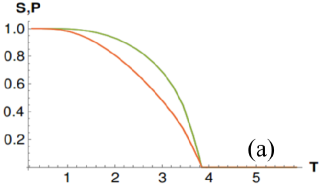
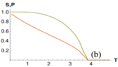
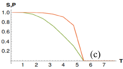
Figure 14: Mean-field results with $J_{mf1}=J_{mf2}\equiv J_{mf}$ (a) Temperature dependence of the magnetization and polarization in the case $J^{m}=1$, $J^{f}=1$, $J_{mf}=-0.12$, $H^{z}=E^{z}=0$. Red lines for the interface $P$ and $M$, green line for the inner layers $M_{2,3}$ and $P_{2,3}$; (b) Temperature dependence of the magnetization and polarization in the case $J^{m}=1$, $J^{f}=1$, $J_{mf}=-0.55$, $H^{z}=0$ and $E^{z}=0$. Red lines for the interface $P$ and $M$, green lines for the inner layers $M_{2,3}$ and $P_{2,3}$; (c) Temperature dependence of the magnetization and polarization in the case $J^{m}=1$, $J^{f}=1$, $J_{mf}=-0.85$, $H^{z}=E^{z}=0$. Red lines for the interface $P$ and $M$, green lines for the inner layers $M_{2,3}$ and $P_{2,3}$. $|\vec{S}|=|P|=1$.

If we compare Figs.  14 and  4-6 one can see an agreement between MC and MF theory that the interface order parameter depends strongly on the interface coupling and have different value from that of the interior layers.

If we take $|P|=1.5$ we see different transition temperatures for magnetic and ferroelectric films as seen in Figure  15.

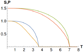
Figure 15: Temperature dependence of the magnetization and polarization for $|\vec{S}|=1$, $|P|=1.5$. $J^{m}=-1$, $J^{f}=1$, $J_{mf}=-0.12$, $H^{z}=E^{z}=0$. Red lines for the interface $P$, gold line for interface $M$, blue line for inner layers $M_{2,3}$ and green line for inner layers $P_{2,3}$.

VI Conclusion

We have studied in this paper the effects of the temperature, external magnetic and electric fields, the magnetoelectric coupling in a multiferroic superlattice formed by alternating magnetic and ferroelectric films. Magnetic films in this work were modeled as films of simple cubic lattice with Heisenberg spins. Electrical polarizations of values $\pm{1}$ were assigned at each lattice site in the ferroelectric films.

We have studied these superlattices with MC simulations and with a MF theory. Various physical quantities have been obtained to identify and characterize the phase transition in each subsystem as functions of temperature $T$, interface coupling parameter and applied magnetic and electric fields. Two models of interface coupling have been considered. The MC and MF calculations agree with each other with regard to the interface order parameters.

Among our MC results let us mention the change of the nature of the phase transition when the interface coupling parameter changes. Various phase diagrams have been established which show that magnetic and ferroelectric phase transitions are closely connected. The interface magnetic and ferroelectric layers have distinct behaviors compared to the inner layers. This is known when there is a loss of translation invariance such as the presence of an impurity, a surface or an interface.

We have worked out a laborious mean-field formalism for superlattices. The application of this in this paper was intentionally limited, but there are wider applications in many system geometries and in various interacting films such as ferri-electric superlattices and frustrated superlattices which have not been considered here.

To conclude, let us emphasize that we have studied in this work two models for interface coupling. Other models of interface magneto-ferroelectric coupling such as the Dzyaloshinskii-Moriya interaction may induce unexpected phenomena at the magneto-ferroelectric interface. Work is under way to investigate this coupling model.

References

References

(1)
H. T. Diep, Theory Of Magnetissm - Application to Surface Physics, World
Scientific, 2014.
(2)
H. T. Diep, Theoretical methods for understanding advanced magnetic materials:
The case of frustrated thin films, Journal of Science: Advanced Materials and
Devices 1 (1) (2016) 31 – 44.
(3)
V. V. Prudnikov, P. V. Prudnikov, D. E. Romanovskii, Monte carlo simulation of
multilayer magnetic structures and calculation of the magnetoresistance
coefficient, JETP Letters 102 (10) (2015) 668–673.
(4)
M. K. Ramazanov, A. K. Murtazaev, Phase transitions in the antiferromagnetic
layered ising model on a cubic lattice, JETP Letters 103 (7) (2016) 460–464.
(5)
I. K. Kamilov, A. K. Murtazaev, K. K. Aliev, Monte carlo studies of phase
transitions and critical phenomena, Physics-Uspekhi 42 (7) (1999) 689–709.
(6)
A. P. Pyatakov, A. K. Zvezdin, Magnetoelectric and multiferroic media,
Physics-Uspekhi 55 (6) (2012) 557–581.
(7)
Y. Weng, L. Lin, E. Dagotto, S. Dong, Inversion of ferrimagnetic magnetization
by ferroelectric switching via a novel magnetoelectric coupling, Phys. Rev.
Lett. 117 (2016) 037601.
(8)
K. Iijima, T. Terashima, Y. Bando, K. Kamigaki, H. Terauchi, Atomic layer
growth of oxide thin films with perovskite‐type structure by reactive
evaporation, Journal of Applied Physics 72 (7).
(9)
D. O’Neill, R. M. Bowman, J. M. Gregg, Dielectric enhancement and
maxwell–wagner effects in ferroelectric superlattice structures, Applied
Physics Letters 77 (10).
(10)
B. D. Qu, W. L. Zhong, R. H. Prince, Interfacial coupling in ferroelectric
superlattices, Phys. Rev. B 55 (1997) 11218–11224.
(11)
R. Ramesh, N. A. Spaldin, Multiferroics: progress and prospects in thin films,
Nature materials 6 (1) (2007) 21–29.
(12)
Y. Magnin, H. T. Diep, Monte carlo study of magnetic resistivity in
semiconducting mnte, Phys. Rev. B 85 (2012) 184413.
(13)
M. K. Kharrasov, I. R. Kyzyrgulov, I. F. Sharafullin, A. G. Nugumanov, Phase
transitions and critical phenomena in multiferroic films with orthorhombic
magnetic structure, Bulletin of the Russian Academy of Sciences: Physics
80 (6) (2016) 695–697.
(14)
I. A. Sergienko, E. Dagotto, Role of the dzyaloshinskii-moriya interaction in
multiferroic perovskites, Phys. Rev. B 73 (2006) 094434.
(15)
I. V. Bychkov, D. A. Kuzmin, V. G. Shavrov, S. Lamekhov, Monte carlo modelling
of two dimensional multiferroics, in: Achievements in Magnetism, Vol. 233 of
Solid State Phenomena, Trans Tech Publications, 2015, pp. 379–382.
(16)
P. M. Leufke, R. Kruk, R. A. Brand, H. Hahn, In situ magnetometry
studies of magnetoelectric lsmo/pzt heterostructures, Phys. Rev. B 87 (2013)
094416.
(17)
H. H. Ortiz-Alvarez, C. M. Bedoya-Hincapie, E. Restrepo-Parra, Monte carlo
simulation of charge mediated magnetoelectricity in multiferroic bilayers,
Physica B: Condensed Matter 454 (2014) 235 – 239.
(18)
V. Y. Irkhin, A new mechanism of first-order magnetization in multisublattice
rare-earth compounds.
(19)
L. Gontchar, A. Nikiforov, Superexchange interaction in insulating manganites r
1- x a x mno 3 (x= 0, 0. 5), Physical Review B 66 (1) (2002) 014437.
(20)
Z. Zhang, et al., Spin waves in several heisenberg systems: Three-sublattice
with different exchange constants (j (ab)= j (bc) not equal j (ca)) and a
superlattice with the elementary unit of four or three different layers.
(21)
H. T. Diep, H. Giacomini, Frustration - exactly solved frustrated models, in:
Frustrated Spin Systems, World Scientific, 2013, pp. 1–58.
(22)
W. Wang, F.-l. Xue, M.-z. Wang, Compensation behavior and magnetic properties
of a ferrimagnetic mixed-spin (1/2, 1) ising double layer superlattice,
Physica B: Condensed Matter 515 (2017) 104–111.
(23)
A. Feraoun, A. Zaim, M. Kerouad, Quantum monte carlo study of the electric
properties of a ferroelectric superlattice, Solid State Communications 248
(2016) 88 – 96.
(24)
D. P. Landau, K. Binder, A guide to Monte Carlo simulations in statistical
physics, Cambridge university press, 2014.
(25)
X. T. P. Phu, V. T. Ngo, H. T. Diep, Crossover from first-to second-order
transition in frustrated ising antiferromagnetic films, Physical Review E
79 (6) (2009) 061106.
(26)
X. T. P. Phu, V. T. Ngo, H. T. Diep, Critical behavior of magnetic thin films,
Surface Science 603 (1) (2009) 109–116.
(27)
H. T. Diep, Quantum theory of helimagnetic thin films, Phys. Rev. B 91 (2015)
014436.
(28)
I. A. Sergienko, E. Dagotto, Role of the dzyaloshinskii-moriya interaction in
multiferroic perovskites, Physical Review B 73 (9) (2006) 094434.
(29)
H. T. Diep, S. El Hog, A. Bailly-Reyre, Skyrmion crystals: Dynamics and phase
transition, AIP Advances 8 (5) (2018) 055707.