Dzyaloshinskii-Moriya Interaction in Magneto-Ferroelectric Superlattices: Spin Waves and Skyrmions

Abstract

We study in this paper effects of Dzyaloshinskii-Moriya (DM) magnetoelectric coupling between ferroelectric and magnetic layers in a superlattice formed by alternate magnetic and ferroelectric films. Magnetic films are films of simple cubic lattice with Heisenberg spins interacting with each other via an exchange $J$ and a DM interaction with the ferroelectric interface. Electrical polarizations of $\pm{1}$ are assigned at simple cubic lattice sites in the ferroelectric films. We determine the ground-state (GS) spin configuration in the magnetic film. In zero field, the GS is periodically non collinear and in an applied field $\mathbf{H}$ perpendicular to the layers, it shows the existence of skyrmions at the interface. Using the Green’s function method we study the spin waves (SW) excited in a monolayer and also in a bilayer sandwiched between ferroelectric films, in zero field. We show that the DM interaction strongly affects the long-wave length SW mode. We calculate also the magnetization at low temperature $T$. We use next Monte Carlo simulations to calculate various physical quantities at finite temperatures such as the critical temperature, the layer magnetization and the layer polarization, as functions of the magnetoelectric DM coupling and the applied magnetic field. Phase transition to the disordered phase is studied in detail.

I Introduction

Non-uniform spin structures, which are quite interesting by themselves, became the subject of close attention after the discovery of electrical polarization in some of them dong2011microscopic . The existence of polarization is possible due to the inhomogeneous magnetoelectric effect, namely that electrical polarization can occur in the region of magnetic inhomogeneity. It is known that the electric polarization vector is transformed in the same way as the combination of the magnetization vector and the gradient of the magnetization vector, meaning that these values can be related by the proportionality relation. In Ref. mostovoy2006ferroelectricity, it was found that in a crystal with cubic symmetry the relationship between electrical polarization and inhomogeneous distribution of the magnetization vector has the following form

$$\mathbf{P}=\gamma\chi_{e}(\mathbf{M}\cdot(\bigtriangledown\cdot\mathbf{M})-(\mathbf{M}\cdot\bigtriangledown)\cdot\mathbf{M})$$ (1)

here $\gamma$ is the magnetoelectric coefficient, and $\chi_{e}$ the permittivity. In non collinear structures, the microscopic mechanism of the coupling of polarization and the relative orientation of the magnetization vectors is based on the interaction of Dzyaloshinskii-Moriya katsura2005spin ; sergienko2006role ; cheong2007multiferroics . The corresponding term in the Hamiltonian is:

$$H_{DM}=\mathbf{D}_{i,j}\cdot\mathbf{S_{i}}\times\mathbf{S_{j}}$$ (2)

where $\mathbf{S_{i}}$ is the spin of the i-th magnetic ion, and $\mathbf{D}_{i,j}$ is the Dzyaloshinskii-Moriya vector. The vector $\mathbf{D}_{i,j}$ is proportional to the vector product $\mathbf{R}\times\mathbf{r_{i,j}}$ of the vector $\mathbf{R}$ which specifies the displacement of the ligand (for example, oxygen) and the unit vector $\mathbf{r_{i,j}}$ along the axis connecting the magnetic ions $i$ and $j$ (see Fig. 1a). We write

$$\mathbf{D}_{i,j}\propto\ \mathbf{R}\times\mathbf{r_{i,j}}$$ (3)

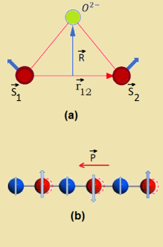
Figure 1: (a) Schema of Dzyaloshinskii-Moriya interaction (b) microscopic mechanisms of creation of electric polarization $\vec{P}$ due to displacements of atoms (red) in the region of inhomogeneous distribution of magnetizations.

Thus, the Dzyaloshinskii-Moriya interaction connects the angle between the spins and the magnitude of the displacement of non-magnetic ions. In some micromagnetic structures all ligands are shifted in one direction, which leads to the appearance of macroscopic electrical polarization (see Fig. 1b). By nature, this interaction is a relativistic amendment to the indirect exchange interaction, and is relatively weak pyatakov2012spin . In the case of magnetically ordered matter, the contribution of the Dzyaloshinskii-Moriya interaction to the free energy can be represented as Lifshitz antisymmetric invariants containing spatial derivatives of the magnetization vector. In analogy, the vortex magnetic configuration can be stable via Skyrme mechanism bogdanov1989thermodynamically . Skyrmions were theoretically predicted more than twenty years ago as stable micromagnetic structures bogdanov1994thermodynamically . The idea came from nuclear physics, where the elementary particles were represented as vortex configurations of continuous fields. The stability of such configurations was provided by the ”Skyrme mechanism” - the components in Lagrangians containing antisymmetric combinations of spatial derivatives of field components skyrme1962unified . For a long time skyrmions have been the subject only of theoretical studies. In particular, it was shown that such structures can exist in antiferromagnets bogdanov2002magnetic and in magnetic metals rossler2006spontaneous . In the latter case, the model included the possibility of changing the magnitude of the magnetization vector and spontaneous emergence of the skyrmion lattice without the application of external magnetic field. A necessary condition for the existence of skyrmions in bulk samples was the absence of an inverse transformation in the crystal magnetic symmetry group. Diep et al. diep2018skyrmion have studied a crystal of skyrmions generated on a square lattice using a ferromagnetic exchange interaction and a Dzyaloshinskii-Moriya interaction between nearest-neighbors under an external magnetic field. They have shown that the skyrmion crystal has a hexagonal structure which is shown to be stable up to a temperature $T_{c}$ where a transition to the paramagnetic phase occurs and the dynamics of the skyrmions at $T<T_{c}$ follows a stretched exponential law. In Ref. rossler2006spontaneous, it was shown that the most extensive class of candidates for the detection of skyrmions includes the surfaces and interfaces of magnetic materials, where the geometry of the material breaks the central symmetry and, therefore, can lead to the appearance of chiral interactions similar to the Dzyaloshinskii-Moriya interaction. In addition, skyrmions are two-dimensional solitons, the stability of which is provided by the local competition of short-range interactions exchange and Dzyaloshinskii-Moriya interactions diep2018skyrmion ; kiselev2011ns . The idea of using skyrmions in memory devices nowadays is reduced to the information encoding using the presence or absence of a skyrmion in certain area of the material. A numerical simulation of the creation and displacement of skyrmions in thin films was carried out in Ref. sampaio2013nucleation, using a spin-polarized current. The advantage of skyrmions with respect to the domain boundaries in such magnetic memory circuits (e.g. racetrack memory, see Ref. parkin2008magnetic, ) is the relatively low magnitude of the currents required to move the skyrmions along the ”track”. For the first time, skyrmions were experimentally detected in the $MnSi$ helimagnet muhlbauer2009skyrmion . Below the Curie temperature in $MnSi$ spins are aligned in helicoidal or conical structure (the field was applied along the $[100]$ axis), depending on the magnitude of the applied magnetic field. Similar experimental results were obtained for the compound $Fe_{1-x}Co_{x}Si,x=0.2$ munzer2010skyrmion . Note here that properties of a helimagnetic thin film with quantum Heisenberg spin model by using the Green’s function method was investigated in Ref. PhysRevB.91.014436, . Surface spin configuration is calculated by minimizing the spin interaction energy. The transition temperature is shown to depend strongly on the helical angle. Results are in agreement with existing experimental observations on the stability of helical structure in thin films and on the insensitivity of the transition temperature with the film thickness.The investigation of $Fe_{0.5}Co_{0.5}Si$ made it possible to take the next important step in the study of skyrmions - to directly observe them using Lorentz electron microscopy yu2010real . The sample was a thin film, magnetic structure of which can be considered two-dimensional: the spatial period of the helicoid (90 nm) exceeded the film thickness, therefore its wave vector laid in the film plane. The magnetic field was applied perpendicular to the film, resulting in suppression of helix and the appearance of the skyrmions lattice. The dependence of the stability of the skyrmion lattice on the sample thickness was studied in more detail in Ref. yu2011near, . A wedge-shaped $FeGe$ sample was created, whose thickness varied from 15 nm to hundreds of nanometers (with a helicoid period of about 70 nm). Studies have confirmed that the thinner was the film, the greater was the ”stability region” of skyrmions. Skyrmions as the most compact isolated micromagnetic objects are of great practical interest as memory elements kiselev2011ns . The stability of skyrmions diep2018skyrmion can make the memory on their basis non-volatile, and low control currents will reduce the cost of rewriting compared to similar technologies based on domain boundaries. In Refs. seki2012observation, ; seki2012magnetoelectric, magnetic and electrical properties of the skyrmion lattice were studied in the multiferroic $Cu_{2}OSeO_{3}$. It has been shown that that energy consumption can be minimized by using the electric field to control the micromagnetic structures. It is worth noting that the multiferroics $BaFe_{12-x-0.05}Sc_{x}Mg_{0.05}O_{19}$ may also have a skyrmion structure yu2012magnetic ; rosch2012extra . The manipulations with skyrmions were first demonstrated in the diatomic $PdFe$ layer on the iridium substrate, and the importance of this achievement for the technology of information storing is difficult to overestimate: it makes possible to write and read the individual skyrmions using a spin-polarized tunneling current romming2013writing . The idea was to apply the magnetic field to the region of the phase diagram corresponding to the intermediate state between the skyrmion lattice and the uniformly magnetized ferromagnetic state. Then, using a needle of a tunneling microscope, a spin-polarized current was passed through various points of the sample, which led to the appearance of skyrmions in the desired positions. In Ref. pyatakov2011magnetically, , the possibility of the nucleation of skyrmions by the electric field by means of an inhomogeneous magnetoelectric effect was established. The required electric field strength can be estimated in order of magnitude as $10^{6}B/cm$, which lies in the range of experimentally achievable values. It is shown that the direction of the electric field determines the chirality of the micromagnetic structure. Recent studies are focused on the interface-induced skyrmions. Therefore, the superstructures naturally lead to the interaction of skyrmions on different interfaces, which has unique dynamics compared to the interaction of the same-interface skyrmions. In Ref. koshibae2017theory, , a theoretical study of two skyrmions on two-layer systems was carried using micromagnetic modeling, as well as an analysis based on the Thiele equation, which revealed a reaction between them, such as the collision and a bound state formation. The dynamics sensitively depends on the sign of DM interaction, i.e. the helicity, and the skyrmion numbers of two skyrmions, which are well described by the Thiele equation. In addition, the colossal spin-transfer-torque effect of bound skyrmion pair on antiferromagnetically coupled bilayer systems was discovered. In Ref. martinez2016topological, the study of the Thiele equation was carried for current-induced motion in a skyrmion lattice through two soluble models of the pinning potential.

We consider in this paper a superlattice composed of alternate magnetic films and ferroelectric films. The aim of this paper is to propose a new model for the coupling between the magnetic film and the ferroelectric film by introducing a DM-like interaction. It turns out that this interface coupling gives rise to non collinear spin configurations in zero applied magnetic field and to skyrmions in a field $\mathbf{H}$ applied perpendicularly to the films. Using the Green’s function method, we study spin-wave excitations in zero field of a monolayer and a bilayer. We find that the DM interaction affects strongly the long wave-length mode. Monte Carlo simulations are carried out to study the phase transition of the superlattice as functions of the interface coupling strength.

The paper is organized as follows. Section II is devoted to the description of our model and the determination of the ground-state spin configuration with and without applied magnetic field. In section III we show the results of the Green’s function technique in zero field for a monolayer and a bilayer. Section IV shows the results obtained by Monte Carlo simulations for the phase transition in the system as a function of the interface DM coupling. Concluding remarks are given in section V.

II Model and ground state

II.1 Model

Consider a superlattice composed of alternate magnetic and ferroelectric films (see Fig. LABEL:ref-fig1b). The Hamiltonian of this multiferroic superlattice is expressed as:

$${\cal H}=H_{m}+H_{f}+H_{mf}$$ (4)

where $H_{m}$ and $H_{f}$ are the Hamiltonians of the ferromagnetic and ferroelectric subsystems, respectively, while $H_{m}f$ is the Hamiltonian of magnetoelectric interaction at the interface between two adjacent films.

We describe the Hamiltonian of the magnetic film with the Heisenberg spin model on a cubic lattice:

$$H_{m}=-\sum_{i,j}{J^{m}_{ij}\mathbf{S}_{i}\cdot\mathbf{S}_{j}}-\sum_{i}\mathbf{H}\cdot\mathbf{S}_{i}$$ (5)

where $\mathbf{S}_{i}$ is the spin on the i-th site, $\mathbf{H}$ is the external magnetic field, $J_{ij}^{m}>0$ the ferromagnetic interaction parameter between a spin and its nearest neighbors (NN) and the sum is taken over NN spin pairs. We consider $J_{ij}^{m}>0$ to be the same, namely $J^{m}$, for spins everywhere in the magnetic film. The external magnetic field $\mathbf{H}$ is applied along the $z$-axis which is perpendicular to the plane of the layers. The interaction of the spins at the interface will be given below.

For the ferroelectric film, we suppose for simplicity that electric polarizations are Ising-like vectors of magnitude 1, pointing in the $\pm z$ direction. The Hamiltonian is given by

$$H_{f}=-\sum_{i,j}{J_{ij}^{f}{\mathbf{P}}_{i}\cdot{\mathbf{P}}_{j}}-\sum_{i}E^{z}P^{z}_{i}$$ (6)

where $\mathbf{P}_{i}$ is the polarization on the i-th lattice site, $J_{ij}^{f}>0$ the interaction parameter between NN and the sum is taken over NN sites. Similar to the ferromagnetic subsystem we will take the same $J_{ij}^{f}=J^{f}$ for all ferroelectric sites. We apply the external electric field $\mathbf{E}$ along the $z$-axis.

We suppose the following Hamiltonian for the magnetoelectric interaction at the interface

$$H_{mf}=\sum_{i,j,k}J_{ijk}^{mf}\ \mathbf{D}_{i,j}\cdot\left[\mathbf{S_{i}}\times\mathbf{{S_{j}}}\right]$$ (7)

In this expression $J_{ijk}^{mf}\ \mathbf{D}_{i,j}$ plays the role of the DM vector which is perpendicular to the $xy$ plane. Using Eqs. (2)-(3), one has

$$\mathbf{D}_{i,j} = \mathbf{R}\times\mathbf{r}_{i,j}$$

$$\mathbf{D}_{j,i} = \mathbf{R}\times\mathbf{r}_{j,i}=-\mathbf{D}_{i,j}$$ (8)

Now, let us define for our model

$$J_{ijk}^{mf}=J_{i,j}^{mf}P_{k}$$ (9)

which is the DM interaction parameter between the electric polarization $\mathbf{P}_{k}$ at the interface ferroelectric layer and the two NN spins $\mathbf{S_{i}}$ and $\mathbf{S_{j}}$ belonging to the interface ferromagnetic layer. Hereafter, we suppose $J_{i,j}^{mf}=J^{mf}$ independent of $(i,j)$. Selecting $\mathbf{R}$ in the $xy$ plane perpendicular to $\mathbf{r}_{i,j}$ (see Fig. 1) we can write $\mathbf{R}\times\mathbf{r}_{i,j}=a\mathbf{z}\ e_{i,j}$ where $e_{i,j}=-e_{j,i}=1$, $a$ is a constant and $\mathbf{z}$ the unit vector on the $z$ axis.

It is worth at this stage to specify the nature of the DM interaction to avoid a confusion often seen in the literature. The term $\left[\mathbf{S}_{i}\times\mathbf{S}_{j}\right]$ changes its sign with the permutation of $i$ and $j$, but the whole DM interaction defined in Eq. (2) does not change its sign because $D_{i,j}$ changes its sign with the permutation as seen in Eq. (3). Note that if the whole DM interaction is antisymmetric then when we perform the lattice sum, nothing of the DM interaction remains in the Hamiltonian. This explains why we need the coefficient $e_{i,j}$ introduced above and present in Eq. (10).

We collect all these definitions we write $H_{mf}$ in a simple form

$$H_{mf} = \sum_{i,j,k}J^{mf}\ P_{k}\ (\mathbf{R}\times\mathbf{r}_{i,j})\cdot\left[\mathbf{S_{i}}\times\mathbf{{S_{j}}}\right]$$ (10)

$$= \sum_{i,j,k}J^{mf}\ P_{k}\ e_{i,j}\mathbf{z}\cdot\left[\mathbf{S_{i}}\times\mathbf{{S_{j}}}\right]$$

$$= \sum_{i,j,k}J^{mf}\ e_{i,j}\ \mathbf{P}_{k}\cdot\left[\mathbf{S_{i}}\times\mathbf{{S_{j}}}\right]$$

where the constant $a$ is absorbed in $J^{mf}$.

The superlattice and the interface interaction are shown in Fig. 2. A polarization at the interface interact with 5 spins on the magnetic layer according to Eq. (10), for example (see Fig. 2b):

$$J^{mf}\mathbf{P}_{1}\cdot[e_{1,2}(\mathbf{S_{1}}\times\mathbf{{S_{2}}})+e_{1,3}(\mathbf{S_{1}}\times\mathbf{{S_{3}}})$$

$$+e_{1,4}(\mathbf{S_{1}}\times\mathbf{{S_{4}}})+e_{1,5}(\mathbf{S_{1}}\times\mathbf{{S_{5}}})]$$ (11)

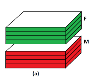
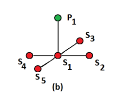
Figure 2: (a) The superlattice composed of alternately a ferroelectric layer indicated by F and a magnetic layer indicated by M; (b) A polarization $P_{1}$ at the interface interacts with 5 spins in the magnetic layer. See text for expression.

Since we suppose $\mathbf{P}_{k}$ is a vector of magnitude 1 pointing along the $z$ axis, namely its $z$ component is $P_{k}^{z}=\pm 1$, we will use hereafter $P_{k}^{z}$ for electric polarization instead of $\mathbf{P}_{k}$.

From Eq. (10), we see that the magnetoelectric interaction $J^{mf}$ favors a canted spin structure. It competes with the exchange interaction $J$ of $H_{m}$ which favors collinear spin configurations. Usually the magnetic or ferroelectric exchange interaction is the leading term in the Hamiltonian, so that in many situations the magnetoelectric effect is negligible. However, in nanofilms of superlattices the magnetoelectric interaction is crucial for the creation of non-collinear long-range spin order.

II.2 Ground state

II.3 Ground state in zero magnetic field

Let us analyze the structure of the ground state (GS) in zero magnetic field. Since the polarizations are along the $z$ axis, the interface DM interaction is minimum when $\mathbf{S_{i}}$ and $\mathbf{S_{j}}$ lie in the $xy$ interface plane and perpendicular to each other. However the ferromagnetic exchange interaction among the spins will compte with the DM perpendicular configuration. The resulting configuration is non collinear. We will determine it below, but at this stage, we note that the ferroelectric film has always polarizations along the $z$ axis even when interface interaction is turned on.

Let us determine the GS spin configurations in magnetic layers in zero field. If the magnetic film has only one monolayer, the minimization of $H^{mf}$ in zero magnetic field is done as follows.

By symmetry, each spin has the same angle $\theta$ with its four NN in the $xy$ plane. The energy of the spin $\mathbf{S}_{i}$ gives the relation between $\theta$ and $J^{m}$

$$E_{i}=-4J^{m}S^{2}\cos\theta+8J^{mf}P^{z}S^{2}\sin\theta$$ (12)

where $\theta=|\theta_{i,j}|$ and care has been taken on the signs of $\sin\theta_{i,j}$ when counting NN, namely two opposite NN have opposite signs, and the oppossite coefficient $e_{ij}$, as given in Eq. (11). Note that the coefficient 4 of the first term is the number of in-plane NN pairs , and the coefficient 8 of the second term is due to the fact that each spin has 4 coupling DM pairs with the NN polarization in the upper ferroelectric plane, and 4 with the NN polarization of the lower ferroelectric plane (we are in the case of a magnetic monolayer). The minimization of $E_{i}$ yields, taking $P^{z}=1$ in the GS and $S=1$,

$$\frac{dE_{i}}{d\theta}=0\ \ \Rightarrow\ \ \frac{-2J^{mf}}{J^{m}}=\tan\theta\ \ \Rightarrow\ \ \theta=\arctan(-\frac{2J^{mf}}{J^{m}})$$ (13)

The value of $\theta$ for a given $\frac{-2J^{mf}}{J^{m}}$ is precisely what obtained by the numerical minimization of the energy. We see that when $J^{mf}\rightarrow 0$, one has $\theta\rightarrow 0$, and when $J^{mf}\rightarrow-\infty$, one has $J^{mf}\rightarrow\pi/2$ as it should be. Note that we will consider in this paper $J^{mf}<0$ so as to have $\theta>0$.

The above relation between the angle and $J^{mf}$ will be used in the next section to calculate the spin waves in the case of a magnetic monolayer sandwiched between ferroelectric films.

In the case when the magnetic film has a thickness, the angle between NN spins in each magnetic layer is different from that of the neighboring layer. It is more convenient using the numerical minimization method called ”steepest descent method” to obtain the GS spin configuration. This method consists in minimizing the energy of each spin by aligning it parallel to the local field acting on it from its NN. This is done as follows. We generate a random initial spin configuration, then we take one spin and calculate the interaction field from its NN. We align it in the direction of this field, and take another spin and repeat the procedure until all spins are considered. We go again for another sweep until the total energy converges to a minimum. In principle, with this iteration procedure the system can be stuck in a meta-stable state when there is a strong interaction disorder such as in spin-glasses. But for uniform, translational interactions, we have never encountered such a problem in many systems studied so far.

We use a sample size $N\times N\times L$. For most calculations, we select $N=40$ and $L=8$ using the periodic boundary conditions in the $xy$ plane. For simplicity, when we investigate the effect of the exchange couplings on the magnetic and ferroelectric properties, we take the same thickness for the upper and lower layers $L_{a}=L_{b}=4=L/2$. Exchange parameters between spins and polarizations are taken as $J^{m}=J^{f}=1$ for the simulation. For simplicity we will consider the case where the in-plane and inter-plane exchange magnetic and ferroelectric interactions between nearest neighbors are both positive. All the results are obtained with $J^{m}=J^{f}=1$ for different values of the interaction parameter $J^{mf}$.

We investigated the following range of values for the interaction parameters $J^{mf}$: from $J^{mf}=-0.05$ to $J^{mf}=-6.0$ with different values of the external magnetic and electric fields. We note that the steepest descent method calculates the real ground state with the minimum energy to the value $J^{mf}=-1.25$. After larger values, the angle $\theta$ tends to $\pi/2$ so that all magnetic exchange terms (scalar products) will be close to zero, the minimum energy corresponds to the DM energy. Figure 3 shows the GS configurations of the magnetic interface layer for small values of $J^{mf}$: -0.1, -0.125, -0.15. Such small values yields small values of angles between spins so that the GS configurations have ferromagnetic and non collinear domains. Note that angles in magnetic interior layers are different but the GS configurations are of the same texture (not shown).

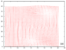
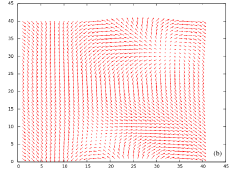
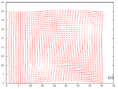
Figure 3: GS spin configuration for weak couplings: $J^{mf}=-0.1$ (a), -0.125 (b), -0.15 (c), with $H=0$

For larger values of $J^{mf}$, the GS spin configurations have periodic structures with no more mixed domains. We show in Fig. 4 examples where $J^{mf}=-0.45$ and -1.2. Several remarks are in order:

i) Each spin has the same turning angle $\theta$ with its NN in both $x$ and $y$ direction. The schematic zoom in Fig. 4c shows that the spins on the same diagonal (spins 1 and 2, spins 3 and 4) are parallel. This explains the structures shown in Figs. 4a and 4b;

ii) The periodicity of the diagonal parallel lines depends on the value of $\theta$ (comparing Fig. 4a and Fig. 4b). With a large size of $N$, the periodic conditions have no significant effects.

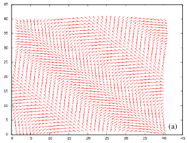
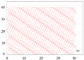
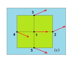
Figure 4: GS spin configurations for $J^{mf}=-0.45$ (a), -1.2 (b), with $H=0$. Angles between NN are schematically zoomed (c). See text for comments.

II.4 Ground state in applied magnetic field

We apply a magnetic field perpendicular to the $xy$ plane. As we know, in systems where some spin orientations are incompatible with the field such as in antiferromagnets, the down spins cannot be turned into the field direction without loosing its interaction energy with the up spins. To preserve this interaction, the spins turn into the direction almost perpendicular to the field while staying almost parallel with each other. This phenomenon is called ”spin flop” DiepTM . In more complicated systems such as helimagnets in a field, more complicated reaction of spins to the field was observed, leading to striking phenomena such as partial phase transition in thin helimagnetic films SahbiHeliField . In the present system, the

Figure 5a shows the ground state configuration for $J^{mf}=-1.1$ for first (surface) magnetic layer, with external magnetic layer $H=0.1$. Figure 5b shows the 3D view. We can observe the beginning of the birth of skyrmions at the interface and in the interior magnetic layer.

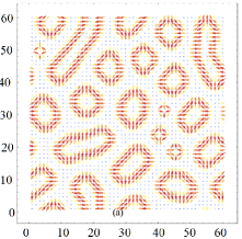
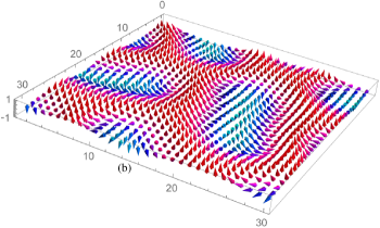
Figure 5: GS configuration of the surface magnetic layer for (a) $J^{mf}=-1.1$ and $H=0.1$, (b) 3D view of the surface GS configuration.

Figure 6a shows the ground state configuration for $J^{mf}=-1.1$ for first (surface) magnetic layer, with external magnetic layer $H=0.2$. Figure 6b shows the 3D view. We can observe the skyrmions for the surface and interior magnetic layer.

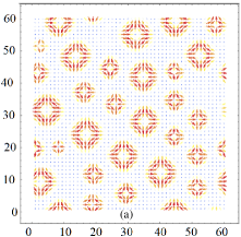
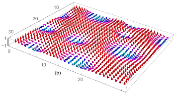
Figure 6: (a) GS configuration for the surface magnetic layer for $J^{mf}=-1.1$ and $H=0.2$, (b) 3D view.

Figure 7 shows the GS configuration of the interface magnetic layer (top) for $J^{mf}=-1.1$, with external magnetic layer $H=0.33$. The bottom figure shows the configurations of the second (interior) magnetic layer. We can observe skyrmions on both the interface and the interior magnetic layers.

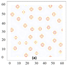
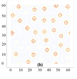
Figure 7: (a) GS configuration for the interface magnetic layer for $J^{mf}=-1.1$ and $H=0.33$, (b) GS configurations for the second and third magnetic layers (they are identical). See text for comments.

Figure 8 shows the 3D view of the GS configuration for $J^{mf}=-1.1$, with $H=0.33$ for the first (interface) magnetic layer and the second (interior) magnetic layer. We can observe skyrmions very pronounced for the surface layer but less contrast for the interior magnetic layer. For fields stronger than $H=0.33$, skyrmions disappear in interior layers. At strong fields, all spins are parallel to the field, thus no skyrmions anywhere.

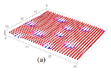
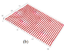
Figure 8: (a) 3D view of the GS configuration of the interface, (b) 3D view of the GS configuration of the second and third magnetic layers, for $J^{mf}$ and $H=0.33$.

III Spin waves in zero field

Before showing Monte Carlo results for the phase transition in our superlattice model, let us show theoretically spin-waves (SW) excited in the magnetic film in zero field, in some simple cases. The method we employ is the Green’s function technique for non collinear spin configurations which has been shown to be efficient for studying low-$T$ properties of quantum spin systems such as helimagnets PhysRevB.91.014436 and systems with a DM interaction SahbiSW .

In this section, we consider the same Hamiltonian supposed in Eqs. (4)-(10) but with quantum spins of amplitude 1/2.

As seen in the previous section, the spins lie in the $xy$ planes, each on its quantization local axis lying in the $xy$ plane (quantization axis being the $\zeta$ axis, see Fig. 9).

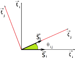
Figure 9: The spin quantization axes of $\mathbf{S}_{i}$ and $\mathbf{S}_{j}$ are $\hat{\zeta}_{i}$ and $\hat{\zeta}_{j}$, respectively, in the $xy$ plane.

Expressing the spins in the local coordinates, one has

$$\mathbf{S}_{i} = S_{i}^{\xi_{i}}\hat{\xi}_{i}+S_{i}^{\eta_{i}}\hat{\eta}_{i}+S_{i}^{\zeta_{i}}\hat{\zeta}_{i}$$ (14)

$$\mathbf{S}_{j} = S_{j}^{\xi_{j}}\hat{\xi}_{j}+S_{j}^{\eta_{j}}\hat{\eta}_{j}+S_{j}^{\zeta_{j}}\hat{\zeta}_{j}$$ (15)

where the $i$ and $j$ coordinates are connected by the rotation

$$\hat{\xi}_{j} = \cos\theta_{ij}\hat{\zeta}_{i}+\sin\theta_{ij}\hat{\xi}_{i}$$

$$\hat{\zeta}_{j} = -\sin\theta_{ij}\hat{\zeta}_{i}+\cos\theta_{ij}\hat{\xi}_{i}$$

$$\hat{\eta}_{j} = \hat{\eta}_{i}$$

where $\theta_{ij}=\theta_{i}-\theta_{j}$ being the angle between $\mathbf{S}_{i}$ and $\mathbf{S}_{j}$.

As we have seen above, the GS spin configuration for one monolayer is periodically non collinear. For two-layer magnetic film, the spin configurations in two layers are identical by symmetry. However, for thickness larger than 2, the interior layer have angles different from that on the interface layer. It is not our purpose to treat that case though it is possible to do so using the method described in Ref. SahbiSW, . We rather concentrate ourselves in the case of a monolayer in this section.

In this paper, we consider the case of spin one-half $S=1/2$. Expressing the total magnetic Hamiltonian $\mathcal{H}_{M}=\mathcal{H}_{m}+\mathcal{H}_{mf}$ in the local coordinates SahbiSW . Writing $\mathbf{S}_{j}$ in the coordinates $(\hat{\xi}_{i},\hat{\eta}_{i},\hat{\zeta}_{i})$, one gets the following exchange Hamiltonian from Eqs. (4)-(10)

$$\mathcal{H}_{M} = -\sum_{<i,j>}J^{m}\Bigg{\{}\frac{1}{4}\left(\cos\theta_{i,j}-1\right)\left(S^{+}_{i}S^{+}_{j}+S^{-}_{i}S^{-}_{j}\right)$$

$$+ \frac{1}{4}\left(\cos\theta_{i,j}+1\right)\left(S^{+}_{i}S^{-}_{j}+S^{-}_{i}S^{+}_{j}\right)$$

$$+ \frac{1}{2}\sin\theta_{i,j}\left(S^{+}_{i}+S^{-}_{i}\right)S^{z}_{j}-\frac{1}{2}\sin\theta_{i,j}S^{z}_{i}\left(S^{+}_{j}+S^{-}_{j}\right)$$

$$+ \cos\theta_{i,j}S^{z}_{i}S^{z}_{j}\Bigg{\}}$$

$$+ \frac{D}{4}\sum_{\left<i,j\right>}[(S_{i}^{+}+S_{i}^{-})(S_{j}^{+}+S_{j}^{-})|\sin\theta_{i,j}|$$

$$+4S_{i}^{z}S_{j}^{z}|\sin\theta_{i,j}|]$$

where $D=J^{mf}P^{z}$. Note that $P^{z}=1$ in the GS. At finite $T$ we replace $P^{z}$ by $<P^{z}>$. In the above equation, we have used standard notations of spin operators for easier recognition when using the commutation relations in the course of calculation, namely

$$(S_{i}^{\xi_{i}},S_{i}^{\eta_{i}},S_{i}^{\zeta_{i}})\rightarrow(S_{i}^{x},S_{i}^{y},S_{i}^{z})$$

$$(S_{j}^{\xi_{j}},S_{j}^{\eta_{j}},S_{j}^{\zeta_{j}})\rightarrow(S_{j}^{x},S_{j}^{y},S_{j}^{z})$$ (17)

where we understand that $S_{i}^{x}$ is in fact $S_{i}^{x_{i}}$ and so on.

Note that the sinus terms of $\mathcal{H}_{m}$, the 3rd line of Eq. (LABEL:eq:HGH2), are zero when summed up on opposite NN unlike the sinus term of the DM Hamiltonian $H_{mf}$, Eq. (10) which remains thanks to the choice of the DM vectors for opposite directions in Eq. SahbiSW .

III.1 Monolayer

In two dimensions (2D) there is no long-range order at finite temperature ($T$) for isotropic spin models with short-range interaction Mermin . Therefore to stabilize the ordering at finite $T$ it is useful to add an anisotropic interaction. We use the following anisotropy between $\mathbf{S}_{i}$ and $\mathbf{S}_{j}$ which stabilizes the angle determined above between their local quantization axes $S^{z}_{i}$ and $S^{z}_{j}$:

$$\mathcal{H}_{a}=-\sum_{<i,j>}K_{i,j}S^{z}_{i}S^{z}_{j}\cos\theta_{i,j}$$ (18)

where $K_{i,j}$ is supposed to be positive, small compared to $J^{m}$, and limited to NN. Hereafter we take $I_{i,j}=K$ for NN pair in the $xy$ plane, for simplicity. The total magnetic Hamiltonian $\mathcal{H}_{M}$ is finally given by (using operator notations)

$$\mathcal{H}_{M}=\mathcal{H}_{m}+\mathcal{H}_{mf}+\mathcal{H}_{a}$$ (19)

We now define the following two double-time Green’s functions in the real space

$$G_{i,j}(t,t^{\prime}) = <<S_{i}^{+}(t);S_{j}^{-}(t^{\prime})>>$$ (20)

$$= -i\theta(t-t^{\prime})<\left[S_{i}^{+}(t),S_{j}^{-}(t^{\prime})\right]>$$

$$F_{i,j}(t,t^{\prime}) = <<S_{i}^{-}(t);S_{j}^{-}(t^{\prime})>>$$ (21)

$$= -i\theta(t-t^{\prime})<\left[S_{i}^{-}(t),S_{j}^{-}(t^{\prime})\right]>$$

The equations of motion of these functions read

$$i\hbar\frac{dG_{i,j}(t,t^{\prime})}{dt} = <\left[S_{i}^{+}(t),S_{j}^{-}(t^{\prime})\right]>\delta(t-t^{\prime})$$ (22)

$$-<<\left[\mathcal{H}_{M},S_{i}^{+}\right];S_{j}^{-}>>$$

$$i\hbar\frac{dF_{i,j}(t,t^{\prime})}{dt} = <\left[S_{i}^{-}(t),S_{j}^{-}(t^{\prime})\right]>\delta(t-t^{\prime})$$ (23)

$$-<<\left[\mathcal{H}_{M},S_{i}^{-}\right];S_{j}^{-}>>$$

For the $\mathcal{H}_{m}$ and $\mathcal{H}_{a}$ parts, the above equations of motion generate terms such as $<<S_{l}^{z}S_{i}^{\pm};S_{j}^{-}>>$ and $<<S_{l}^{\pm}S_{i}^{\pm};S_{j}^{-}>>$. These functions can be approximated by using the Tyablikov decoupling to reduce to the above-defined $G$ and $F$ functions:

$$<<S_{l}^{z}S_{i}^{\pm};S_{j}^{-}>>\simeq<S_{l}^{z}><<S_{i}^{\pm};S_{j}^{-}>>$$ (24)

$$<<S_{l}^{\pm}S_{i}^{\pm};S_{j}^{-}>>\simeq<S_{l}^{\pm}><<S_{i}^{\pm};S_{j}^{-}>>\simeq 0$$ (25)

The last expression is due to the fact that transverse spin-wave motions $<S_{l}^{\pm}>$ are zero with time. For the DM term, the commutation relations $[\mathcal{H},S_{i}^{\pm}]$ give rise to the following term:

$$D\sum_{l}\sin\theta[\mp S_{i}^{z}(S_{l}^{+}+S_{l}^{-})\pm 2S_{i}^{\pm}S_{l}^{z}]$$ (26)

This leads to the following type of Green’s function:

$$<<S_{i}^{z}S_{l}^{\pm};S_{j}^{-}>>\simeq<S_{i}^{z}><<S_{l}^{\pm};S_{j}^{-}>>\\$$ (27)

Note that we have used defined $\theta$ positively. The above equation is thus related to $G$ and $F$ functions [see Eq. (25)].

We use the following Fourier transforms in the $xy$ plane of the $G$ and $F$ Green’s functions:

$$G_{i,j}(t,t^{\prime},\omega) = \frac{1}{\Delta}\int_{BZ}d{\mathbf{k}_{xy}}\mbox{e}^{-i\hbar\omega(t-t^{\prime})}g(\omega,\mathbf{k}_{xz})\mbox{e}^{i\mathbf{k}_{xy}.(\mathbf{R}_{i}-\mathbf{R}_{j})}$$ (28)

$$F_{i,j}(t,t^{\prime},\omega) = \frac{1}{\Delta}\int_{BZ}d{\mathbf{k}_{xy}}\mbox{e}^{-i\hbar\omega(t-t^{\prime})}f(\omega,\mathbf{k}_{xy})\mbox{e}^{i\mathbf{k}_{xy}.(\mathbf{R}_{i}-\mathbf{R}_{j})}$$ (29)

where the integral is performed in the first $xy$ Brillouin zone (BZ) of surface $\Delta$ and $\omega$ is the SW frequency. Let us define the SW energy as $E=\hbar\omega$ in the following.

For a monolayer, we have after the Fourier transforms

$$(E+A)g+Bf = 2<S^{z}>$$

$$-Bg+(E-A)f = 0$$ (30)

where $A$ and $B$ are

$$A = -J^{m}[8<S^{z}>\cos\theta(1+d)-4<S^{z}>\gamma(\cos\theta+1)]$$ (31)

$$-4D\sin\theta<S^{z}>\gamma+8D\sin\theta<S^{z}>$$

$$B = 4J^{m}<S^{z}>\gamma(\cos\theta-1)-4D\sin\theta<S^{z}>\gamma$$ (32)

where the reduced anisotropy is $d=K/J^{m}$ and $\gamma=(\cos k_{x}a+\cos k_{y}a)/2$, $k_{x}$ and $k_{y}$ being the wave-vector components in the $xy$ planes, $a$ the lattice constant.

The SW energies are determined by the secular equation

$$(E+A)(E-A)+B^{2}=0$$

$$[E+A][E-A]+B^{2}=0$$

$$E^{2}-A^{2}+B^{2}=0$$

$$E=\pm\sqrt{(A+B)(A-B)}$$ (33)

where $\pm$ indicate the left and right SW precessions. We see that

• if $\theta=0$, we have $B$ and the last two terms of $A$ are zero. We recover then the ferromagnetic SW dispersion relation

  $$E=2ZJ^{m}<S^{z}>(1-\gamma)$$ (34)

  where $Z=4$ is the coordination number of the square lattice (taking $d=0$),

• if $\theta=\pi$, we have $A=8J^{m}<S^{z}>$ and $B=-8J^{m}<S^{z}>\gamma$. We recover then the antiferromagnetic SW energy

  $$E=2ZJ^{m}<S^{z}>\sqrt{1-\gamma^{2}}$$ (35)

• in the presence of a DM interaction, we have $0<\cos\theta<1$ ($0<\theta<\pi/2$). If $d=0$, the quantity in the square root of Eq. (33) is always $\geq 0$ for any $\theta$. It is zero at $\gamma=1$. We do not need an anisotropy $d$ to stabilize the SW at $T=0$. If $d=\neq zero$ then it gives a gap at $\gamma=1$.

We show in Fig. 10 the SW energy calculated from Eq. (33) for $\theta=0.3$ radian ($\simeq 17.2$ degrees) and 1 radian ($\simeq 57.30$ degrees). The spectrum is symmetric for positive and negative wave vectors and for left and right precessions. Note that for small values of $\theta$ (i. e. small $D$) $E$ is proportional to $k^{2}$ at low $k$ (cf. Fig. 10a), as in ferromagnets. However, for strong $\theta$, $E$ is proportional to $k$ as seen in Fig. 10b. This behavior is similar to that in antiferromagnets DiepTM . The change of behavior is progressive with increasing $\theta$, no sudden transition from $k^{2}$ to $k$ behavior is observed.

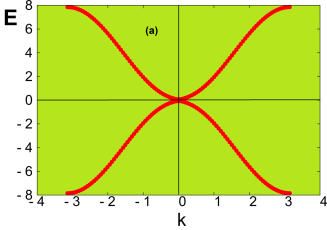
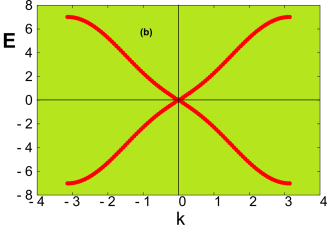
Figure 10: Spin-wave energy $E(k)$ versus $k$ ($k\equiv k_{x}=k_{z}$) for (a) $\theta=0.3$ radian and (b) $\theta=1$ in 2D at $T=0$. See text for comments.

In the case of $S=1/2$, the magnetization is given by (see technical details in Ref. DiepTM, ):

$$\langle S^{z}\rangle=\frac{1}{2}-\frac{1}{\Delta}\int\int dk_{x}dk_{y}[\frac{1}{\mbox{e}^{E_{i}/k_{B}T}-1}+\frac{1}{\mbox{e}^{-E_{i}/k_{B}T}-1}]$$ (36)

where for each $\mathbf{k}$ one has $\pm E_{i}$ values.

Since $E_{i}$ depends on $S^{z}$, the magnetization can be calculated at finite temperatures self-consistently using the above formula.

It is noted that the anisotropy $d$ avoids the logarithmic divergence at $k=0$ so that we can observe a long-range ordering at finite $T$ in 2D. We show in Fig. 11 the magnetization $M$ ($\equiv<S^{z}>$) calculated by Eq. (36) for using $d=0.001$. It is interesting to observe that $M$ depends strongly on $\theta$: at high $T$, larger $\theta$ yields stronger $M$. However, at $T=0$ the spin length is smaller for larger $\theta$ due to the so-called spin contraction in antiferromagnets DiepTM . As a consequence there is a cross-over of magnetizations with different $\theta$ at low $T$ as shown in Fig. 11.

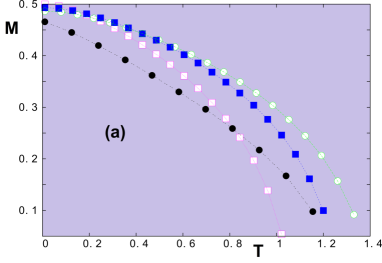
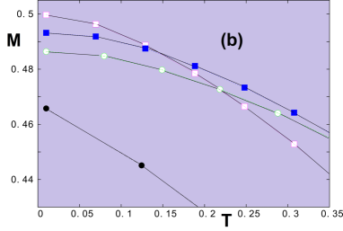
Figure 11: (a) Spin length $M=<S^{z}>$ versus temperature $T$ for a 2D sheet with $\theta=0.175$ (radian) (magenta void squares), $\theta=0.524$ (blue filled squares), $\theta=0.698$ (green void circles), $\theta=1.047$ (black filled circles); (b) Zoom at low $T$ to show magnetization cross-overs.

The spin length at $T=0$ is shown in Fig. 12 for several $\theta$.

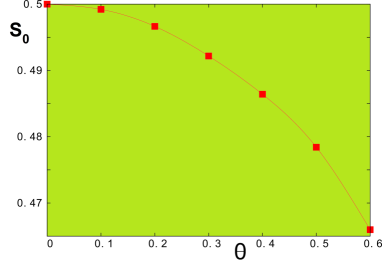
Figure 12: Spin length at temperature $T=0$ for a monolayer versus $\theta$ (radian).

III.2 Bilayer

We note that for magnetic bilayer between two ferroelectric films, the calculation similar to that of a monolayer can be done. By symmetry, spins between the two layers are parallel, the energy of a spin on a layer is

$$E_{i}=-4J^{m}S^{2}\cos\theta-J^{m}S^{2}+4J^{mf}P^{z}S^{2}\sin\theta$$ (37)

where there are 4 in-plane NN and one parallel NN spin on the other layer. The interface coupling is with only one polarization instead of two (see Eq. (12)) for a monolayer for comparison.

The minimum energy corresponds to $\tan\theta=-J^{mf}/J^{m}$.

The calculation by the Green’s functions for a film with a thickness is straightforward: writing the Green’s functions for each layer and making Fourier transforms in the $xy$ planes, we obtain a system of coupled equations. For the details, the reader is referred to Ref. PhysRevB.91.014436, . For a bilayer, the SW energy is the eigenvalues of the following matrix equation

$$\mathbf{M}\left(E\right)\mathbf{h}=\mathbf{u},$$ (38)

where

$$\mathbf{h}=\left(\begin{array}[]{c}g_{1,n^{\prime}}\\ f_{1,n^{\prime}}\\ g_{2,n^{\prime}}\\ f_{2,n^{\prime}}\\ \end{array}\right),\hskip 28.45274pt\mathbf{u}=\left(\begin{array}[]{c}2\left<S^{z}_{1}\right>\delta_{1,n^{\prime}}\\ 0\\ 2\left<S^{z}_{2}\right>\delta_{2,n^{\prime}}\\ 0\\ \end{array}\right),$$ (39)

where $E=\hbar\omega$ and $\mathbf{M}\left(E\right)$ is given by

$$\left(\begin{array}[]{cccc}E+A_{1}&B_{1}&C_{1}&0\\ -B_{1}&E-A_{1}&0&-C_{1}\\ C_{2}&0&E+A_{2}&B_{2}\\ 0&-C_{2}&-B_{2}&E-A_{2}\\ \end{array}\right)$$ (40)

with

$$A_{1} = -J^{m}[8<S^{z}_{1}>\cos\theta(1+d)-4<S^{z}_{1}>\gamma(\cos\theta+1)]$$ (41)

$$-2J^{m}<S^{z}_{2}>-4D\sin\theta<S^{z}_{1}>\gamma+8D\sin\theta<S^{z}_{1}>$$

$$A_{2} = -J^{m}[8<S^{z}_{2}>\cos\theta(1+d)-4<S^{z}_{2}>\gamma(\cos\theta+1)]$$ (42)

$$-2J^{m}<S^{z}_{1}>-4D\sin\theta<S^{z}_{2}>+8D\sin\theta<S^{z}_{2}>$$

$$B_{n} = 4J^{m}<S^{z}_{n}>\gamma(\cos\theta-1)-4D\sin\theta<S^{z}_{n}>\gamma,\ \ \ n=1,2$$ (43)

$$C_{n} = 2J^{m}<S^{z}_{n}>,\ \ \ n=1,2$$ (44)

Note that by symmetry, one has $<S^{z}_{1}>=<S^{z}_{2}>$.

We show in Fig. 13 the SW spectrum of the bilayer case for a strong value $\theta=0.6$ radian. There are two important points:

(i) the first mode has the $E\propto k$ antiferromagnetic behavior at the long wave-length limit for this strong $\theta$,

(ii) the higher mode has $E\propto k^{2}$ which is the ferromagnetic wave due to the parallel NN spins in the $z$ direction.

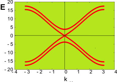
Figure 13: Spin-wave energy $E$ versus $k=k_{x}=k_{y}$ at $T=0$ for a bilayer with $\theta=0.6$ radian.

In conclusion of this section, we emphasize that the DM interaction affects strongly the SW mode at $k\rightarrow 0$. Quantum fluctuations in competition with thermal effects cause the cross-over of magnetizations of different $\theta$: in general stronger $\theta$ yields stronger spin contraction at and near $T=0$ so that the corresponding spin length is shorter. However at higher $T$, stronger $\theta$ means stronger $J^{mf}$ which yields stronger magnetization. It explains the cross-over at moderate $T$.

IV Monte Carlo results

We have used the Metropolis algorithm Landau09 ; Brooks11 to calculate physical quantities of the system at finite temperatures $T$. As said above, we use mostly the size $N\times N\times L$ with $N=40$ and thickness $L=L_{m}+L_{f}=8$ (4 magnetic layers, 4 ferroelectric layers). Simulation times are $10^{5}$ Monte Carlo steps (MCS) per spin for equilibrating the system and $10^{5}$ MCS/spin for averaging. We calculate the internal energy and the layer order parameters of the magnetic ($M_{m}$) and ferroelectric ($M_{f}$) films.

The order parameter $M_{f}(n)$ of layer $n$ is defined as

$$M_{f}(n)=\frac{1}{N^{2}}\langle{|\sum_{i\in n}P_{i}^{z}|}\rangle$$ (45)

where $\langle{...}\rangle$ denotes the time average.

The definition of an order parameter for a skyrmion crystal is not obvious. Taking advantage of the fact that we know the GS, we define the order parameter as the projection of an actual spin configuration at a given $T$ on its GS and we take the time average. This order parameter of layer $n$ is thus defined as

$$M_{m}(n)=\frac{1}{N^{2}(t_{a}-t_{0})}\sum_{i\in n}|\sum_{t=t_{0}}^{t_{a}}\mathbf{S}_{i}(T,t)\cdot\mathbf{S}_{i}^{0}(T=0)|$$ (46)

where $\mathbf{S}_{i}(T,t)$ is the $i$-th spin at the time $t$, at temperature $T$, and $\mathbf{S}_{i}(T=0)$ is its state in the GS. The order parameter $M_{m}(n)$ is close to 1 at very low $T$ where each spin is only weakly deviated from its state in the GS. $M_{m}(n)$ is zero when every spin strongly fluctuates in the paramagnetic state. The above definition of $M_{m}(n)$ is similar to the Edward-Anderson order parameter used to measure the degree of freezing in spin glasses Mezard : we follow each spin with time evolving and take the spatial average at the end. The total order parameters $M_{m}$ and $M_{f}$ are the sum of the layer order parameters, namely $M_{m}=\sum_{n}M_{m}(n)$ and $M_{f}=\sum_{n}M_{f}(n)$.

In Fig.14 we show the dependence of energy of the magnetic film versus temperature, without an external magnetic field, for various values of the interface magnetoelectric interaction: in Fig.14a for weak values $J^{mf}=-0.1,J^{mf}=-0.125,J^{mf}=-0.15,J^{mf}=-0.2$, and in Fig.14b for stronger values $J^{mf}=-0.45,J^{mf}=-0.75,J^{mf}=-0.85,J^{mf}=-1.2$.

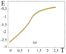
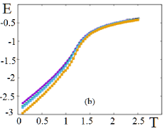
Figure 14: Energy of the magnetic film versus temperature $T$ for (a) $J^{mf}=-0.1,J^{mf}=-0.125,J^{mf}=-0.15,J^{mf}=-0.2$ (all the lines are the same, see text for comments); (b) $J^{mf}=-0.45$ (purple line), $J^{mf}=-0.75$ (green line), $J^{mf}=-0.85$ (blue line) and $J^{mf}=-1.2$ (gold line), without an external magnetic field.

As said in the GS determination, when $J^{mf}$ is weak, the GS is composed with large ferromagnetic domains at the interface (see Fig. 3). Interior layers are still ferromagnetic. The energy is therefore does not vary with weak values of $J^{mf}$ as seen in Fig. LABEL:6a. The phase transition occurs at the curvature change, namely maximum of the derivative or maximum of the specific heat, $T_{c}^{m}\simeq 1.25$. Note that the energy at $T=0$ is equal to -2.75 by extrapolating the curves in Fig. 14a to $T=0$. This value is just the sum of energies of the spins across the layers: 2 interior spins with 6 NN, 2 interface spins with 2 NN. The energy per spin is thus (in ferromagnetic state): $E=-(2\times 6+2\times 5)/(4\times 2)=-2.75$ (the factor 2 in the denominator is to remove the bond double counting in a crystal).

For stronger values of $J^{mf}$, the curves shown in Fig. 14b indicate a deviation of the ferromagnetic state due to the non collinear interface structure. Nevertheless, we observe the magnetic transition at almost the same temperature, namely $T_{c}^{m}\simeq 1.25$. It means that spins in interior layers dominate the ordering.

We show in Fig. 15 the total order parameters of the magnetic film $M_{m}$ and the ferroelectric film $M_{f}$ versus $T$ for various values of the parameter of the magnetoelectric interaction $J^{mf}=-0.1,-0.125,-0.15,-0.2$ and for $J^{mf}=-0.45,-0.75,-0.85,-1.2$, without an external magnetic field. Several remarks are in order:

i) For the magnetic film, $M_{m}$ shows strong fluctuations but we still see that all curves fall to zero at $T_{c}^{m}\simeq 1.25$. These fluctuations come from non uniform spin configurations and also from the nature of the Heisenberg spins in low dimensions Mermin .

ii) For the ferroelectric film, $M_{f}$ behaves very well with no fluctuations. This is due to the Ising nature of electric polarizations supposed in the present model. The ferroelectric film undergoes a phase transition at $T_{c}^{f}\simeq 1.50$.

iii) There are thus two transitions, one magnetic and one ferroelectric, separately.

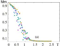
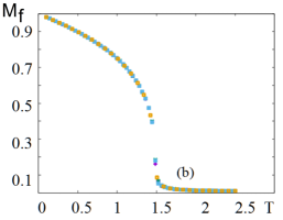
Figure 15: (a) Order parameter of the magnetic film $M_{m}$ versus $T$; (b) Order parameter of the ferroelectric film $M_{f}$ versus $T$, for $J^{mf}=-0.1$ (purple dots), $J^{mf}=-0.125$ (green dots), $J^{mf}=-0.15$ (blue dots), $J^{mf}=-0.2$ (gold dots), without an external magnetic field.

We show in Fig. 16 the order parameters of the magnetic and ferroelectric films at strong values of $J^{mf}$ as functions of $T$, in zero field. We observe that the stronger $J^{mf}$ is, the lower $T_{c}^{m}$ becomes.The ferroelectric $T_{c}^{f}$ does not change as expected.

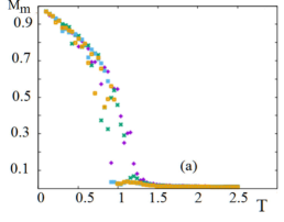
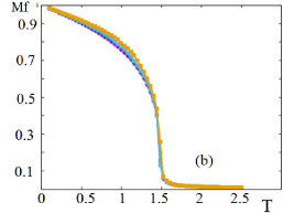
Figure 16: (a) Order parameter of the magnetic film versus $T$; (b) Order parameter of the ferroelectric film versus $T$ for $J^{mf}=-0.45$ (purple dots), $J^{mf}=-0.75$ (green dots), $J^{mf}=-0.85$ (blue dots) and $J^{mf}=-1.2$ (gold dots), without an external magnetic field.

We examine the field effects now. Figure 17 shows the order parameter and the energy of the magnetic film versus $T$, for various values of the external magnetic field. The interface magnetoelectric interaction is $J^{mf}=-1.2$. Depending on the magnetic field, the non collinear spin configuration survives up to a temperature between 0.5 and 1 (for $H=0$). After the transition, spins align themselves in the field direction, giving a large value of the order parameter (Fig. 17a). The energy shows a sharp curvature change only for $H=0$, meaning that the specific heat is broadened more and more with increasing $H$.

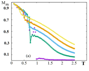
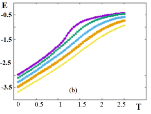
Figure 17: (a) Temperature dependence of (a) the magnetic order parameter; (b) the magnetic energy for $H=0$ (purple dots), $H=0.25$ (green line), $H=0.5$ (blue line), $H=0.75$ (gold line), $H=1$ (yellow line). The interface magnetoelectric interaction is $J^{mf}=-1.2$.

We consider now the case of very strong interface couplings.

Figure 18a shows the magnetic order parameter versus $T$. The purple and green lines correspond to $M$ for $J^{m}f=-2.5$ with $H^{z}=1.0$ and $H^{z}=1.5$, respectively; the blue and gold lines correspond to $M$ for $J^{mf}=-6$ with $H^{z}=0$ and $H^{z}=1$. These curves indicate first-order phase transitions at $T_{c}^{m}=1.05$ for $(J^{mf}=-2.5,H^{z}=1)$ (purple), at $T_{c}^{m}=1.12$ for $(J^{mf}=-2.5,H^{z}=1.5$) (green) and at $T_{c}^{m}=2.25$ for $(J^{mf}=-6,H^{z}=1)$ (gold). In the case of zero field, namely $(J^{mf}=-6,H^{z}=0)$ (blue), one has two first-order phase transitions occurring at $T_{c1}=1.05$ and $T_{c2}=2.19$.

Figure 18b shows the magnetic (purple) and ferroelectric (green) energies versus $T$ for $(J^{mf}=-6,H^{z}=0)$. One sees the discontinuities of these curves at $T_{c}\simeq 2.29$, indicating the first-order transitions for both magnetic and ferroelectric at the same temperature. In fact, with such a strong $J^{mf}$ the transitions in both magnetic and ferroelectric films are driven by the interface, this explains the same $T_{c}$ for both.

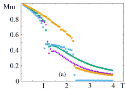
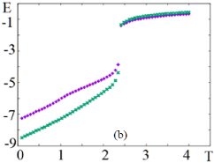
Figure 18: (a) Order parameter of magnetic film versus $T$. The purple and green dots correspond to $M$ for $(J^{mf}=-2.5,H^{z}=1)$ and $(J^{mf}=-2.5,H^{z}=1.5$), blue and gold dots correspond to $M$ for $(J^{mf}=-6,H^{z}=1)$ and $(J^{mf}=-6,H^{z}=0)$. (b) Energies of magnetic (purple dots) and ferroelectric (green dots) subsystems versus $T$ for $(J^{mf}=-6,H=0)$.

Let us show the effect of an applied electric field. For the ferroelectric film, polarizations are along the $z$ axis so that an applied electric field $\mathbf{E}$ along this direction will remove the phase transition: the order parameter never vanishes when $E\neq 0$. This is seen in Fig. 19. Note that the energy has a sharp change of curvature for $E=0$ indicating a transition, other energy curves with $E\neq 0$ do not show a transition. One notices some anomalies at $T\sim 1-1.1$ which are due to the effect of the magnetic transition in this temperature range.

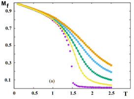
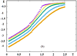
Figure 19: (a) Order parameter and (b) energy of ferroelectric film, versus temperature for $E=0$ (purple dots), $E=0.25$ (green line), $E=0.5$ (blue line), $E=0.75$ (gold line), $E=1$ (yellow line). The interface magnetoelectric interaction is $J^{mf}=-1.2$

V Conclusion

We have studied in this paper a new model for the interface coupling between a magnetic film and a ferroelectric film in a superlattice. This coupling has the form of a Dzyaloshinskii-Moriya (DM) interaction between a polarization and the spins at the interface.

The ground state shows uniform non collinear spin configurations in zero field and skyrmions in an applied magnetic field. We have studied spin-wave (SW) excitations in a monolayer and in a bilayer in zero field by the Green’s function method. We have shown the strong effect of the DM coupling on the SW spectrum as well as on the magnetization at low temperatures.

Monte Carlo simulation has been used to study the phase transition occurring in the superlattice with and without applied field. Skyrmions have been shown to be stable at finite temperatures. We have also shown that the nature of the phase transition can be of second or first order, depending on the DM interface coupling.

The existence of skyrmions confined at the magneto-ferroelectric interface is very interesting. We believe that it can be used in transport applications in spintronic devices. A number of applications using skyrmions has been already mentioned in the Introduction.

References

References

- (1) S. Dong, X. Zhang, R. Yu, J.-M. Liu, E. Dagotto, Microscopic model for the ferroelectric field effect in oxide heterostructures, Physical Review B 84 (15) (2011) 155117.
- (2) M. Mostovoy, Ferroelectricity in spiral magnets, Physical Review Letters 96 (6) (2006) 067601.
- (3) H. Katsura, N. Nagaosa, A. V. Balatsky, Spin current and magnetoelectric effect in noncollinear magnets, Physical review letters 95 (5) (2005) 057205.
- (4) I. A. Sergienko, E. Dagotto, Role of the dzyaloshinskii-moriya interaction in multiferroic perovskites, Physical Review B 73 (9) (2006) 094434.
- (5) S.-W. Cheong, M. Mostovoy, Multiferroics: a magnetic twist for ferroelectricity, Nature materials 6 (1) (2007) 13.
- (6) A. Pyatakov, A. Zvezdin, A. Vlasov, A. Sergeev, D. Sechin, E. Nikolaeva, A. Nikolaev, H. Chou, S. Sun, L. Calvet, Spin structures and domain walls in multiferroics spin structures and magnetic domain walls in multiferroics, Ferroelectrics 438 (1) (2012) 79–88.
- (7) A. N. Bogdanov, D. Yablonskii, Thermodynamically stable vortices in magnetically ordered crystals. the mixed state of magnets, Zh. Eksp. Teor. Fiz 95 (1) (1989) 178.
- (8) A. Bogdanov, A. Hubert, Thermodynamically stable magnetic vortex states in magnetic crystals, Journal of magnetism and magnetic materials 138 (3) (1994) 255–269.
- (9) T. H. R. Skyrme, A unified field theory of mesons and baryons, Nuclear Physics 31 (1962) 556–569.
- (10) A. Bogdanov, U. Rößler, M. Wolf, K.-H. Müller, Magnetic structures and reorientation transitions in noncentrosymmetric uniaxial antiferromagnets, Physical Review B 66 (21) (2002) 214410.
- (11) U. Rößler, A. Bogdanov, C. Pfleiderer, Spontaneous skyrmion ground states in magnetic metals, Nature 442 (7104) (2006) 797.
- (12) H. T. Diep, S. El Hog, A. Bailly-Reyre, Skyrmion crystals: Dynamics and phase transition, AIP Advances 8 (5) (2018) 055707.
- (13) N. Kiselev, Ns kiselev, an bogdanov, r. schäfer, and uk rößler, j. phys. d 44, 392001 (2011)., J. Phys. D 44 (2011) 392001.
- (14) J. Sampaio, V. Cros, S. Rohart, A. Thiaville, A. Fert, Nucleation, stability and current-induced motion of isolated magnetic skyrmions in nanostructures, Nature nanotechnology 8 (11) (2013) 839.
- (15) S. S. Parkin, M. Hayashi, L. Thomas, Magnetic domain-wall racetrack memory, Science 320 (5873) (2008) 190–194.
- (16) S. Mühlbauer, B. Binz, F. Jonietz, C. Pfleiderer, A. Rosch, A. Neubauer, R. Georgii, P. Böni, Skyrmion lattice in a chiral magnet, Science 323 (5916) (2009) 915–919.
- (17) W. Münzer, A. Neubauer, T. Adams, S. Mühlbauer, C. Franz, F. Jonietz, R. Georgii, P. Böni, B. Pedersen, M. Schmidt, et al., Skyrmion lattice in the doped semiconductor fe 1- x co x si, Physical Review B 81 (4) (2010) 041203.
- (18) H. T. Diep, Quantum theory of helimagnetic thin films, Phys. Rev. B 91 (2015) 014436.
- (19) X. Yu, Y. Onose, N. Kanazawa, J. Park, J. Han, Y. Matsui, N. Nagaosa, Y. Tokura, Real-space observation of a two-dimensional skyrmion crystal, Nature 465 (7300) (2010) 901.
- (20) X. Yu, N. Kanazawa, Y. Onose, K. Kimoto, W. Zhang, S. Ishiwata, Y. Matsui, Y. Tokura, Near room-temperature formation of a skyrmion crystal in thin-films of the helimagnet fege, Nature materials 10 (2) (2011) 106.
- (21) S. Seki, X. Yu, S. Ishiwata, Y. Tokura, Observation of skyrmions in a multiferroic material, Science 336 (6078) (2012) 198–201.
- (22) S. Seki, S. Ishiwata, Y. Tokura, Magnetoelectric nature of skyrmions in a chiral magnetic insulator cu 2 oseo 3, Physical Review B 86 (6) (2012) 060403.
- (23) X. Yu, M. Mostovoy, Y. Tokunaga, W. Zhang, K. Kimoto, Y. Matsui, Y. Kaneko, N. Nagaosa, Y. Tokura, Magnetic stripes and skyrmions with helicity reversals, Proceedings of the National Academy of Sciences 109 (23) (2012) 8856–8860.
- (24) A. Rosch, Extra twist in magnetic bubbles, Proceedings of the National Academy of Sciences 109 (23) (2012) 8793–8794.
- (25) N. Romming, C. Hanneken, M. Menzel, J. E. Bickel, B. Wolter, K. von Bergmann, A. Kubetzka, R. Wiesendanger, Writing and deleting single magnetic skyrmions, Science 341 (6146) (2013) 636–639.
- (26) A. Pyatakov, D. Sechin, A. Sergeev, A. Nikolaev, E. Nikolaeva, A. Logginov, A. Zvezdin, Magnetically switched electric polarity of domain walls in iron garnet films, EPL (Europhysics Letters) 93 (1) (2011) 17001.
- (27) W. Koshibae, N. Nagaosa, Theory of skyrmions in bilayer systems, Scientific Reports 7 (2017) 42645.
- (28) J. Martinez, M. Jalil, Topological dynamics and current-induced motion in a skyrmion lattice, New Journal of Physics 18 (3) (2016) 033008.
- (29) H. T. Diep, Theory Of Magnetissm - Application to Surface Physics, World Scientific, 2014.
- (30) S. El Hog, H. T. Diep, Partial phase transition and quantum effects in helimagnetic films under an applied field, J. Magnetism and Magnetic Materials 429 (2017) 102.
- (31) S. El Hog, H. T. Diep, H. Puszkarski, Theory of magnons in spin systems with dzyaloshinskii-moriya interaction, J. Phys. Condensed Matter 29 (2017) 305001.
- (32) N. D. Mermin, H. Wagner, Phys. Rev. Lett. 17 (1966) 1133.
- (33) D. P. Landau, K. Binder, A Guide to Monte Carlo Simulations in Statistical Physics , Cambridge University Press, London, 2009.
- (34) S. Brooks, A. Gelman, S. L. Jones, X.-L. Meng, Handbook of Markov Chain Monte Carlo, CRC Press, 2011.
- (35) M. Mézard, M. Parisi, M. Virasoro, Spin Glass Theory and Beyond An Introduction to the Replica Method and Its Applications , World Scientific, 1986.