Bi-Linear Modeling of Data Manifolds for Dynamic-MRI Recovery

Abstract

This paper puts forth a novel bi-linear modeling framework for data recovery via manifold-learning and sparse-approximation arguments and considers its application to dynamic magnetic-resonance imaging (dMRI). Each temporal-domain MR image is viewed as a point that lies onto or close to a smooth manifold, and landmark points are identified to describe the point cloud concisely. To facilitate computations, a dimensionality reduction module generates low-dimensional/compressed renditions of the landmark points. Recovery of high-fidelity MRI data is realized by solving a non-convex minimization task for the linear decompression operator and affine combinations of landmark points which locally approximate the latent manifold geometry. An algorithm with guaranteed convergence to stationary solutions of the non-convex minimization task is also provided. The aforementioned framework exploits the underlying spatio-temporal patterns and geometry of the acquired data without any prior training on external data or information. Extensive numerical results on simulated as well as real cardiac-cine MRI data illustrate noteworthy improvements of the advocated machine-learning framework over state-of-the-art reconstruction techniques.

I Introduction

Magnetic-resonance imaging (MRI), a non-invasive, non-ionizing and high-fidelity visualization technology, has found widespread applications in cardiac-cine, dynamic contrast-enhanced and neuro-imaging, playing a key role in medical research and diagnosis [1]. MRI’s inherent limitations and various physiological constraints often incur slow data acquisition, while long scanning times make MRI an expensive process, may cause patient discomfort, and hinder thus its usefulness.

Raw MRI data are observed in the k-space domain; the image (visual) data are computed by the inverse Fourier transform of the k-space ones [1]. A prominent way to speed up data acquisition is to sample the k-space or frequency domain densely enough to ensure reconstruction of a high-fidelity and artifact-free image via Fourier-transform arguments [2]. In the case of dynamic (d)MRI, where an extra-temporal dimension is added to the spatial domain, sampling is also performed along the time axis. Due to MRI’s slow scanning times, it becomes difficult for the data acquisition process to keep up with the motion of the organs or the fluid flow in the field of view (FOV) [1]. It is a usual case to not be able to reach the necessary sampling density, not only in the temporal direction but also in the k-space domain, to guarantee artifact-free reconstructed images. This “under-sampling” inflicts signal aliasing and distortion [3].

Naturally, a lot of the MRI-research effort has been focusing on developing reconstruction algorithms that improve the spatio-temporal resolution of MR images given the highly under-sampled k-space data. To this end, artificial-intelligence (AI) approaches have been very recently placed at the focal point of MRI research; examples are convolutional neural networks (CNNs) [4, 5, 6, 7, 8, 9], deep variational networks(VNs) [10], and generative adversarial neural networks (GANs) [11, 12]. AI methods learn non-linear mappings via extensive offline training on large-scale datasets, different from or in addition to the acquired data, and use those learned non-linear mappings to map the observed low-resolution, or, undersampled data to their high-fidelity counterparts. In contrast to the data-driven AI methods, the present work, as well as the following prior-art schemes, assume no offline training on large-scale datasets and resort solely to the observed data.

A popular approach to exploit the underlying spatio-temporal patterns within dMRI data is compressed sensing (CS) [13, 14, 15, 16]. Low-rank structures [17, 18] and total-variation-based schemes [19, 20, 21] have also been explored at length and found to produce promising results for slow varying dynamic data. For instance, [18] proposes the estimation, first, of a temporal basis of image time series via singular-value decomposition, prior to formulating a sparsity inducing convex-recovery task. Nevertheless, these schemes seem to be less effective when it comes to dMRI with extensive inter-frame motion or with a low number of temporal frames, as mentioned in [22, 23]. Acceleration capabilities of CS combined with the motion-robustness of radial imaging techniques have also found their place in MRI reconstruction and have shown promising results in cardiac and respiratory motion correction. The motion resolved strategy [24] introduces extra motion dimensions by sorting the continuously acquired k-space data into distinct motion states followed by a sparsity and total variation based CS technique for reconstruction. There has also been a growing interest in MRI-recovery by dictionary-learning (DL) schemes [25, 26, 27, 28, 29]. In [23], for example, the dMRI data are decomposed in two components: A low-rank one, that captures the temporal (video) background, and a sparse one, described via spatio-temporal patch-based DL that models the (dynamic) foreground.

Manifold-learning techniques have also been employed to recover dMRI data from highly under-sampled observations [30, 22, 31, 32, 33, 34, 35]. In [22], a graph-Laplacian matrix is formed via the Euclidean distances between points of a data cloud and is subsequently used as a regularizer in a convex-recovery task. Improving on [22], a bandlimited modeling of the data points, coupled with an improved estimation of the Laplacian matrix, was proposed in [31] to make the reconstruction resilient to noise and patient motion, computationally inexpensive and less demanding memory-wise. The work in [32] proposes a kernel variation to the graph Laplacian estimation in [22]. A popular path followed by manifold-learning schemes is to perform dimensionality reduction of the collected high-dimensional data prior to applying a reconstruction algorithm, e.g., [33, 34]. In the non-MRI context, [36] capitalizes, also, on a Euclidean-distance-based Laplacian matrix to perform dimensionality reduction prior to reconstructing data by local principal component analysis. In the previous schemes, all of the observed points participate in the dimensionality-reduction task, raising thus computational burdens, especially in cases where the number of data is excessively large. Methods that perform dimensionality reduction on properly chosen small-cardinality subsets of the observed data cloud have been introduced for clustering and classification, but not for regression tasks [37, 38, 39].

This paper follows the manifold-learning path and serves a two-fold objective: i) Present a machine-learning framework, the bi-linear modeling of data manifolds (BiLMDM), that contributes novelties to exploiting local and latent data structures via a sparsity-aware and bi-linear optimization task; and ii) apply BiLMDM to the dMRI-data recovery problem. In a nutshell, BiLMDM can be described as follows. Each vector of data, observed from an undersampled dMRI temporal frame, is modeled as a point onto or close to an unknown manifold, embedded in a Euclidean space. The only assumption imposed on the manifold is smoothness [40]. Landmark points are chosen to concisely describe the observed data-vector cloud, and are mapped to a lower-dimensional space, as in [34, 41], to effect compression and enable low-computational footprints in the proposed algorithmic solutions. Motivated by the smooth-manifold hypothesis, the proposed work approximates each data vector as an affine combinations of neighboring landmark points (cf. Fig. 2). A locally bi-linear factorization model, novel for data representations, is then formed to model/fit the point cloud: One factor gathers the coefficients of the previous affine combinations of the landmark points, while the other one serves as the linear decompression operator that unfolds the points back to the image dimensions. Improving on our preliminary results [42], a highly modular bi-linear optimization task is tailored to the dMRI-data recovery problem, penalized by terms which account for sparsity along the temporal axis and other modeling assumptions. A successive-convex-approximation algorithm is proposed to guarantee convergence to a stationary solution of the previous bi-linear optimization task.

The proposed work is validated against the following state-of-the-art schemes: Partially separable sparsity aware model (PS-Sparse) [18], joint manifold learning and sparsity aware (MLS) framework [34], smoothness regularization on manifolds (SToRM) [22], low rank and adaptive sparse signal model (LASSI) [23] and extra dimensional golden angle radial sparse parallel (XD-GRASP) [24]. In spite of sharing with the previous state-of-the-art schemes the principle of identifying low-dimensional structures for high-dimensional data and exploiting this structure to reconstruct data, BiLMDM’s original contributions in data approximations can be summarized as follows: i) BiLMDM departs from the mainstream manifold-learning approach of identifying a data-graph Laplacian matrix that penalizes an optimization (data-recovery) task as in [31, 22, 35], and uses instead the fundamental geometric principle of tangent spaces of smooth manifolds to search for data dependencies/patterns through local affine combinations of landmark points (cf. Fig. 2); ii) it offers a novel bi-linear factorization model, where one linear factor captures the local smoothness of the manifolds, via local affine combinations, while the other one accounts for the linear decompression operator which maps the low-dimensional affine approximations back to the high-dimensional raw-data/input space. The affine combinations and the decompression operator are jointly identified via a highly modular non-convex data recovery task, which may accommodate also additional prior information, e.g., periodicity over the temporal axis of the dMRI data. Unlike the traditional bi-linear schemes, BiLMDM doesn’t follow the classical dictionary learning approach of decomposing the image into two components as discussed earlier and model the dynamic foreground of the image as a sparse combination of adaptive dictionary atoms (which act as image basis) of MR image signals. A more detailed description of the differences of BiLMDM with the state-of-the-art dMRI recovery schemes is deferred to Sec. III. The efficacy of BiLMDM was observed on both synthetically generated and experimentally acquired cardiac cine MR data, undersampled via both Cartesian and radial trajectories. BiLMDM has consistently outperformed all the competing techniques and produced reconstructions which were sharp, free of undesirable artifacts, deformations and temporal bleeding.

The rest of the paper is organized as follows: Section II-A describes, in short, the dMRI acquisition scheme in the k-space domain. Section II-B details the BiLMDM’s modeling assumptions, while Sec. III describes the algorithm to solve the proposed non-convex minimization task. The extensive numerical tests of Section IV showcase that BiLMDM outperforms state-of-the-art dMRI recovery schemes. The manuscript summarises the numerical results in Section V and concludes in Section VI. Finally, the appendix gathers basic mathematical facts and expressions that are essential for the implementation of the algorithm described in Sec. III.

II Bi-Linear Modeling of Data Manifolds

II-A dMRI data description

(a)

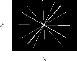
(b)

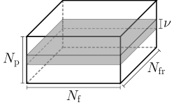
(c)

Figure 1: LABEL:sub@fig:sampling.strategy.cartesian k-space with 1-D Cartesian sampling pattern; LABEL:sub@fig:sampling.strategy.radial k-space with radial sampling pattern; LABEL:sub@fig:DataCube The $N_{\text{p}}\times N_{\text{f}}\times N_{\text{fr}}$ (k,t)-space. “Navigator (pilot) data” comprise the gray-colored $\nu\times N_{\text{f}}\times N_{\text{fr}}$ area of the (k,t)-space ($\nu\ll N_{\text{p}}$).

MRI data $\bm{\mathcal{Y}}\in\mathbb{C}^{N_{\text{p}}\times N_{\text{f}}}$ ($\mathbb{C}$ denotes the set of all complex-valued numbers) are observed in k-space (frequency domain), which spans an area of size $N_{\text{p}}\times N_{\text{f}}$ (cf. Figs. 1a and 1b), with $N_{\text{p}}$ standing for the number of phase-encoding lines and $N_{\text{f}}$ for the number of frequency-encoding ones [1]. Data $\bm{\mathcal{Y}}$ can be considered as the two-dimensional (discrete) Fourier transform $\mathcal{F}(\cdot)$ of the image-domain data $\bm{\mathcal{X}}\in\mathbb{C}^{N_{\text{p}}\times N_{\text{f}}}$, i.e., $\bm{\mathcal{Y}}=\mathcal{F}(\bm{\mathcal{X}})$ [1]. Without any loss of generality, this study assumes that the “low-frequency” part of $\bm{\mathcal{Y}}$ is located around the center of the $N_{\text{p}}\times N_{\text{f}}$ area. Availability of the data over the whole k-space is infeasible in practice; k-space is usually severely under-sampled [3]. There exist several strategies to sample the k-space; examples are the 1-D Cartesian (Fig. 1a) and the radial (Fig. 1b) ones, where the “white” lines in Figs. 1a and 1b denote the available/sampled data, while data in the “black” areas are not observed. A general trend among sampling strategies is to put more emphasis on low-frequency components, which carry contrast information and with high SNR, and select few high-frequency components, which comprise high-resolution image details. The 1-D Cartesian sampling pattern emulates the acquisition of k-space pixels via the 1-D Gaussian distribution, acquiring a large number of samples in the central k-space area while sampling few ones from the “high-frequency” area (cf. Fig. 1a). The radial-sampling pattern consists of radial spokes which yield dense sampling at the center of k-space, while the sampling density is decreased as the spokes move away from the center (cf. Fig. 1b).

In dMRI, an additional dimension is added to the MRI k-space to accommodate time (the axis vertical on the paper in Fig. 1c), resulting in the augmented (k,t)-space. The dMRI (k,t)-space can be viewed, in other words, as the $N_{\text{fr}}$-fold Cartesian product of the $(N_{\text{p}}\times N_{\text{f}})$-sized MRI k-space, where $N_{\text{fr}}$ represents the number of observed MRI frames over time. In dMRI, k-space $\bm{\mathcal{Y}}_{j}$ and image-domain $\bm{\mathcal{X}}_{j}$ data are connected via $\bm{\mathcal{Y}}_{j}=\mathcal{F}(\bm{\mathcal{X}}_{j})$, $j\in\{1,\ldots,N_{\text{fr}}\}$. The (k,t) space is usually highly under-sampled. To extract reliable information from the (k,t)-space data, this work follows [22, 18, 34] and considers a small number $\nu$ ($\ll N_{\text{p}}$) of phase-encoding lines, coined "navigator (pilot) data" (the gray-colored area in Fig. 1c), to learn the intrinsic low-dimensional structure of the data.

To facilitate processing, the (k,t)-space data are vectorized. More specifically, $\operatorname{vec}(\bm{\mathcal{Y}}_{j})$ stacks one column of $\bm{\mathcal{Y}}_{j}$ below the other to yield the complex-valued $N_{\text{k}}\times 1$ vector $\mathbf{y}_{j}:=\operatorname{vec}(\bm{\mathcal{Y}}_{j})$ where $N_{\text{k}}:=N_{\text{p}}N_{\text{f}}$ denotes the number of pixels in every frame. To avoid notation clutter, $\mathcal{F}$ still denotes the two-dimensional (discrete) Fourier transform even when applied to vectorized versions of image frames: $\mathcal{F}[\operatorname{vec}(\bm{\mathcal{X}}_{j})]:=\operatorname{vec}[\mathcal{F}(\bm{\mathcal{X}}_{j})]=\operatorname{vec}(\bm{\mathcal{Y}}_{j})$. All vectorized k-space frames are gathered in the $N_{\text{k}}\times N_{\text{fr}}$ matrix $\mathbf{Y}:=[\mathbf{y}_{1},\mathbf{y}_{2},\ldots,\mathbf{y}_{N_{\text{fr}}}]$ so that the vectorized image-domain data are $\mathbf{X}:=\mathcal{F}^{-1}(\mathbf{Y}):=[\mathcal{F}^{-1}(\mathbf{y}_{1}),\mathcal{F}^{-1}(\mathbf{y}_{2}),\ldots,\mathcal{F}^{-1}(\mathbf{y}_{N_{\text{fr}}})]$, where $\mathcal{F}^{-1}(\cdot)$ denotes the inverse two-dimensional (discrete) Fourier transform. The navigator data of the $j$th k-space frame (cf. Fig. 1c), $j\in\{1,2,\ldots,N_{\text{fr}}\}$, are gathered into a $\nu N_{\text{f}}\times 1$ vector $\mathbf{y}_{j}^{\text{nav}}$. All navigator data comprise the $\nu N_{\text{f}}\times N_{\text{fr}}$ matrix $\mathbf{Y}_{\text{nav}}:=[\mathbf{y}_{1}^{\text{nav}},\mathbf{y}_{2}^{\text{nav}},\ldots,\mathbf{y}_{N_{\text{fr}}}^{\text{nav}}]$.

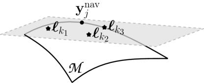
Figure 2: Landmark points $\{\bm{\ell}_{k_{i}}\}_{i=1}^{3}$ are affinely combined to describe $\mathbf{y}_{j}^{\text{nav}}$. All affine combinations of $\{\bm{\ell}_{k_{i}}\}_{i=1}^{3}$ are depicted by the gray-colored plane.

II-B Modeling assumptions

The high-dimensional navigator data $\{\mathbf{y}_{j}^{\text{nav}}\}_{j=1}^{N_{\text{fr}}}$ carry useful information about spatio-temporal dependencies in the (k,t)-space. To promote parsimonious data representations, especially in cases where $N_{\text{fr}}$ attains large values, it is desirable to extract a subset $\{\bm{\ell}_{k}\}_{k=1}^{N_{\ell}}\subset\{\mathbf{y}_{j}^{\text{nav}}\}_{j=1}^{N_{\text{fr}}}$ ($N_{\ell}\leq N_{\text{fr}}$), called landmark points, which provide a “concise description,” in a user-defined sense, of the data cloud $\{\mathbf{y}_{j}^{\text{nav}}\}_{j=1}^{N_{\text{fr}}}$. To this end, the following assumption, often met in manifold-learning approaches [43], imposes structure on $\{\mathbf{y}_{j}^{\text{nav}}\}_{j=1}^{N_{\text{fr}}}$.

Assumption 1.

Data $\{\mathbf{y}_{j}^{\text{nav}}\}_{j=1}^{N_{\text{fr}}}$ lie on a smooth low-dimensional manifold $\mathpzc{M}$ [40] embedded in the high-dimensional Euclidean space $\mathbb{C}^{\nu N_{\text{f}}}$ (cf. Fig. 2).

For example, the most well-known case of $\mathpzc{M}$ is a linear subspace, which is the main hypothesis behind principal component analysis (PCA). PCA assumes that the data lie close to or onto a linear subspace in a low-dimensional space. Along the same lines, based on As. 1 and the concept of the tangent space of a smooth manifold, it is conceivable that neighbouring landmark points cooperate affinely to describe vector $\mathbf{y}_{j}^{\text{nav}}$ (the gray-colored area in Fig. 2 depicts all possible affine combinations of $\{\bm{\ell}_{k_{1}},\bm{\ell}_{k_{2}},\bm{\ell}_{k_{3}}\}$). In other words, every temporal frame is approximated by a combination of landmark points, where these landmark points can be viewed as a representative of a particular group of frames sharing similar phase and motion characteristics. Upon defining the $\nu N_{\text{f}}\times N_{\ell}$ matrix $\bm{\Lambda}:=[\bm{\ell}_{1},\bm{\ell}_{2},\ldots,\bm{\ell}_{N_{\ell}}]$, the above notion can be established by the existence of an $N_{\ell}\times 1$ vector $\mathbf{b}_{j}$ that renders the approximation error $\lVert\mathbf{y}_{j}^{\text{nav}}-\bm{\Lambda}\mathbf{b}_{j}\rVert$ small, where $\lVert\cdot\rVert$ denotes the standard Euclidean norm of space $\mathbb{C}^{\nu N_{\text{f}}}$. Since affine combinations are desirable, $\mathbf{b}_{j}$ is constrained to satisfy $\mathbf{1}_{N_{\ell}}^{\intercal}\mathbf{b}_{j}=1$, where $\mathbf{1}_{N_{\ell}}$ stands for the all-one $N_{\ell}\times 1$ vector and superscript $\intercal$ denotes vector/matrix transposition. Moreover, motivated by the low-dimensional nature of $\mathpzc{M}$ (As. 1), only a few landmark points are considered to cooperate to represent $\mathbf{y}_{j}^{\text{nav}}$ in its closed vicinity, i.e., $\mathbf{b}_{j}$ is sparse. The previous arguments are summarized into the following modeling hypothesis.

Assumption 2.

There exist a sparse $N_{\ell}\times N_{\text{fr}}$ matrix $\mathbf{B}$, with $\mathbf{1}_{N_{\ell}}^{\intercal}\mathbf{B}=\mathbf{1}_{N_{\text{fr}}}^{\intercal}$, and a $\nu N_{\text{f}}\times N_{\text{fr}}$ matrix $\mathbf{E}_{2}$, which gathers approximation errors, such that (s.t.) $\mathbf{Y}_{\text{nav}}=\bm{\Lambda}\mathbf{B}+\mathbf{E}_{2}$.

The previous assumption holds true in the prototypical case where $\mathpzc{M}$ is a linear subspace and $\mathbf{Y}_{\text{nav}}$ comprises column vectors which lie close to or onto $\mathpzc{M}$. Any matrix which includes as column vectors any basis of $\mathpzc{M}$ may serve as $\bm{\Lambda}$. Since the affine hull [44] of the columns of $\bm{\Lambda}$ coincides with $\mathpzc{M}$, there exists surely a coefficient matrix $\mathbf{B}$ that satisfies the affine constraints $\mathbf{1}_{N_{\ell}}^{\intercal}\mathbf{B}=\mathbf{1}_{N_{\text{fr}}}^{\intercal}$ and $\mathbf{Y}_{\text{nav}}=\bm{\Lambda}\mathbf{B}$. It is not now difficult to see that As. 2 covers also the case where $\mathpzc{M}$ is a union $\cup_{q=1}^{Q}\mathpzc{M}_{q}$ of linear subspaces $\{\mathpzc{M}_{q}\}_{q=1}^{Q}$, with $\mathbf{Y}_{\text{nav}}$ comprising columns vectors which lie close to or onto $\{\mathpzc{M}_{q}\}_{q=1}^{Q}$. Hence, As. 2 lays the foundations for more general cases where data vectors lie close to or onto a union of smooth manifolds, with different dimensions. In such a way, As. 2 offers theoretical support and justification in cases where data comprise disparate groups, where intra-group dependencies can be captured by a single smooth manifold, while inter-group relations can be only viewed via the union of those manifolds, e.g., the union of data drawn from a static gray-colored background and data describing the movement of a beating heart.

Although several strategies may be implemented to identify the landmark points $\bm{\Lambda}$, a greedy optimization methodology, introduced in [39], is adopted here. In short, at every step of the algorithm, a landmark point is selected from $\{\mathbf{y}_{j}^{\text{nav}}\}_{j=1}^{N_{\text{fr}}}$ that maximizes, over all un-selected $\{\mathbf{y}_{j}^{\text{nav}}\}_{j=1}^{N_{\text{fr}}}$, the minimum distance to the landmark points which have been already selected up to the previous step of the algorithm. The algorithm of [39] scores a computational complexity of order $\mathcal{O}(N_{\ell}N_{\text{fr}})$, which is naturally heavier than that of a procedure that selects $\{\bm{\ell}_{k}\}_{k=1}^{N_{\ell}}$ randomly from $\{\mathbf{y}_{j}^{\text{nav}}\}_{j=1}^{N_{\text{fr}}}$.

Still, the landmark points (columns of $\bm{\Lambda}$) are high dimensional. To meet restrictions imposed by finite computational resources, it is desirable to reduce the dimensionality of $\bm{\Lambda}$. To this end, the methodology of [41], which is motivated by [43, 45], is employed. The approach comprises of two steps:

1. Given $\bm{\Lambda}$ and a user-defined $\lambda_{W}>0$, solve

   $$\min_{\mathbf{W}\in\mathbb{C}^{N_{\ell}\times N_{\ell}}} \left\lVert\bm{\Lambda}-\bm{\Lambda}\mathbf{W}\right\rVert_{\text{F}}^{2}+\lambda_{W}\lVert\mathbf{W}\rVert_{1}$$

   s.to $$\mathbf{1}_{N_{\ell}}^{\intercal}\mathbf{W}=\mathbf{1}_{N_{\ell}}^{\intercal}\ \text{and}\ \operatorname{diag}(\mathbf{W})=\mathbf{0}\,,$$ (1a)

   where $\lVert\cdot\rVert_{\text{F}}$ stands for the Frobenius norm of a matrix. Since $\{\bm{\ell}_{k}\}_{k=1}^{N_{\ell}}$ lie on the manifold $\mathpzc{M}$, then according to As. 1 and Fig. 2, any point taken from $\{\bm{\ell}_{k}\}_{k=1}^{N_{\ell}}$ may be faithfully approximated by an affine combination of the rest of the landmark points. In other words, there exists a matrix $\mathbf{W}$ s.t. $\bm{\Lambda}\approx\bm{\Lambda}\mathbf{W}$. With $\mathbf{1}_{N_{\ell}}^{\intercal}\mathbf{W}=\mathbf{1}_{N_{\ell}}^{\intercal}$ manifesting the previous desire for affine combinations, the constraint $\operatorname{diag}(\mathbf{W})=\mathbf{0}$ is used to exclude the trivial solution of the identity matrix $\mathbf{I}_{N_{\ell}}$ for $\mathbf{W}$. Task (1a) is an affinely constrained composite convex minimization task, and, hence, the framework of [46] can be employed to solve it, due to the flexibility by which [46] deals with affine constraints when compared with state-of-the-art convex optimization techniques.

2. Once $\mathbf{W}$ is obtained from the previous step and for a user-defined integer number $d\leq\min\{N_{\ell},\nu N_{\text{f}}\}$, solve

   $$\min_{\check{\bm{\Lambda}}\in\mathbb{C}^{d\times N_{\ell}}} \lVert\check{\bm{\Lambda}}-\check{\bm{\Lambda}}\mathbf{W}\rVert_{\text{F}}^{2}\ \text{s.to}\ \check{\bm{\Lambda}}\check{\bm{\Lambda}}^{\mathsf{H}}=\mathbf{I}_{d}\,,$$ (1b)

   where the constraint $\check{\bm{\Lambda}}\check{\bm{\Lambda}}^{\mathsf{H}}=\mathbf{I}_{d}$ is used to exclude the trivial solution of $\check{\bm{\Lambda}}=\mathbf{0}$, and the superscript $\mathsf{H}$ denotes the Hermitian transpose of a matrix. The solution of the previous task is nothing but the complex conjugate transpose of the matrix which comprises the $d$ minimal eigenvectors of $(\mathbf{I}_{N_{\ell}}-\mathbf{W})(\mathbf{I}_{N_{\ell}}-\mathbf{W})^{\mathsf{H}}$.

To this point, the identified landmark points were used to capture a latent structure of the MR data cloud and the structure was further used to compress the landmark points to a lower dimension, thus, facilitating the search for affine combinations in a lower dimensional space. However, there arises a need to unfold the points back to the dimensions of the navigator data which leads us to the following model.

Assumption 3.

There exist an $N_{\text{k}}\times d$ matrix $\mathbf{G}_{3}$ and an $N_{\text{k}}\times N_{\ell}$ matrix $\mathbf{E}_{3}$, which gathers all approximation errors, s.t. $\bm{\Lambda}=\mathbf{G}_{3}\check{\bm{\Lambda}}+\mathbf{E}_{3}$.

Matrix $\mathbf{G}_{3}$ can be viewed as the “decompression” operator which reconstructs the “full” $\bm{\Lambda}$ from its low-dimensional representation $\check{\bm{\Lambda}}$.

The relationship between the undersampled k-space frames and navigator frames can be established, for the case of Fig. 1c, as $\mathbf{Y}_{\text{nav}}=\bm{\Omega}\mathbf{Y}$, where $\bm{\Omega}$ is a matrix with binary entries $\{0,1\}$ that select entries of $\mathbf{Y}$. The inverse problem of recovering $\mathbf{Y}$ from its partial $\mathbf{Y}_{\text{nav}}$ is viable under errors, e.g., an approximation of $\mathbf{Y}$ can be obtained via $\bm{\Omega}^{\dagger}\mathbf{Y}_{\text{nav}}$, where the decompressor $\bm{\Omega}^{\dagger}$ stands for the Moore-Penrose pseudo-inverse of $\bm{\Omega}$. The following modeling hypothesis generalizes this argument.

Assumption 4.

There exist an $N_{\text{k}}\times\nu N_{\text{f}}$ matrix $\mathbf{G}_{1}$ and an $N_{\text{k}}\times N_{\text{fr}}$ matrix $\mathbf{E}_{1}$, which gathers all approximation errors, s.t. $\mathbf{Y}=\mathbf{G}_{1}\mathbf{Y}_{\text{nav}}+\mathbf{E}_{1}$.

A similar modeling assumption can be found in the classical principal component analysis (PCA) [47], where $\mathbf{G}_{1}$ serves as the “decompression” operator (usually an orthogonal matrix) that maps the “compressed” $\mathbf{Y}_{\text{nav}}$ back to the original data $\mathbf{Y}$ under the approximation error $\mathbf{E}_{1}$. However, PCA identifies best-linear-fit approximations to data, which might be an inappropriate modeling assumption for several types of data [43]. The following discussion departs from PCA and establishes modeling assumptions that allow non-linear data geometries.

Putting modeling assumptions 2, 3 and 4 together, it can be verified that there exist matrices $\mathbf{G}$ and $\mathbf{E}$ s.t. $\mathbf{Y}=\mathbf{G}\check{\bm{\Lambda}}\mathbf{B}+\mathbf{E}$. Upon defining $\mathbf{U}:=\mathcal{F}^{-1}(\mathbf{G})$, and since $\mathbf{G}\check{\bm{\Lambda}}\mathbf{B}=\mathcal{F}(\mathbf{U})\check{\bm{\Lambda}}\mathbf{B}=\mathcal{F}(\mathbf{U}\check{\bm{\Lambda}}\mathbf{B})$, by virtue of the linearity of $\mathcal{F}$, the following bi-linear model between $\mathbf{Y}$ and the unknowns $(\mathbf{U},\mathbf{B})$ is established:

$$\mathbf{Y}=\mathcal{F}(\mathbf{U}\check{\bm{\Lambda}}\mathbf{B})+\mathbf{E}\,.$$ (2)

Bi-linearity means that if $\mathbf{U}$ (or $\mathbf{B}$) is fixed to a specific value, then $\mathbf{Y}$ is linear with respect to $\mathbf{B}$ (or $\mathbf{U}$), modulo the error $\mathbf{E}$ term. Interestingly, the linearity of $\mathcal{F}^{-1}$ suggests that the previous modeling hypothesis holds true also in the image domain: $\mathcal{F}^{-1}(\mathbf{Y})=\mathbf{U}\check{\bm{\Lambda}}\mathbf{B}+\mathcal{F}^{-1}(\mathbf{E})$.

III The Bi-Linear Recovery task and its Algorithmic Solution

In practice, only few (k,t)-space data are known. To explicitly take account of the limited number of data, a (linear) sampling/masking operator $\mathcal{S}(\cdot)$ is introduced, where $\mathcal{S}(\mathbf{Y})$ leaves the entries of $\mathbf{Y}$ as they are at sampled or observed positions of the k-space domain while nullifying all the rest. The sampling operator is capable of mimicking any sampling strategy, such as Cartesian, radial, spiral, etc. It is also often in dMRI that image frames capture a periodic process, e.g., heart movement, other than the static background. In other words, it is reasonable to assume that in (2), the one-dimensional Fourier transform $\mathcal{F}_{t}$ of the $1\times N_{\text{fr}}$ time profile of every one of the $N_{\text{k}}$ pixels, i.e., every row of the matrix $\mathcal{F}_{t}(\mathbf{U}\check{\bm{\Lambda}}\mathbf{B})$, is a sparse vector.

All of the previous modeling assumptions are incorporated in the following recovery task: Given the positive real-valued parameters $\lambda_{1},\lambda_{2},\lambda_{3},C_{U}$, solve

$$\min_{(\mathbf{U},\mathbf{B},\mathbf{Z})} \ \overbrace{\tfrac{1}{2}\left\lVert\mathcal{S}(\mathbf{Y})-\mathcal{S}\mathcal{F}(\mathbf{U}\check{\bm{\Lambda}}\mathbf{B})\right\rVert_{\text{F}}^{2}}^{\text{T1}}+\overbrace{\tfrac{\lambda_{1}}{2}\left\lVert\mathbf{Z}-\mathcal{F}_{t}(\mathbf{U}\check{\bm{\Lambda}}\mathbf{B})\right\rVert_{\text{F}}^{2}}^{\text{T2}}$$

$$\ +\underbrace{\lambda_{2}\left\lVert\mathbf{Z}\right\rVert_{1}}_{\text{T3}}+\underbrace{\lambda_{3}\left\lVert\mathbf{B}\right\rVert_{1}}_{\text{T4}}$$

s.to $$\ \underbrace{\left\lVert\mathbf{Ue}_{i}\right\rVert\leq C_{U},\ \forall i\in\{1,\ldots,d\}}_{\text{C1}};~{}\underbrace{\mathbf{1}_{N_{\ell}}^{\intercal}\mathbf{B}=\mathbf{1}_{N_{\text{fr}}}^{\intercal}}_{\text{C2}};$$

$$\mathbf{U}\in\mathbb{C}^{N_{\text{k}}\times d};\mathbf{B}\in\mathbb{C}^{N_{\ell}\times N_{\text{fr}}};\mathbf{Z}\in\mathbb{C}^{N_{\text{k}}\times N_{\text{fr}}},$$ (3)

where $\mathbf{e}_{i}$ denotes the $i$th column of the identity matrix $\mathbf{I}_{d}$. Elaborating more on the recovery task (3), T1 corresponds to the data-fit term, while T2 and T3 introduce the auxiliary variable $\mathbf{Z}$, used to impose a sparsity constraint on $\mathcal{F}_{t}(\mathbf{U}\check{\bm{\Lambda}}\mathbf{B})$. T4 imposes a sparsity constraint on $\mathbf{B}$, following the discussion on As. 2. Bound $C_{U}$ in C1 is used to prevent unbounded solutions for $\mathbf{U}$ due to the scaling ambiguity in the bi-linear term $\mathbf{U}\check{\bm{\Lambda}}\mathbf{B}$. C2 adds the affine constraint discussed in As. 2. Moreover, it is worth noticing here that the reduction of dimensionality, achieved via $\check{\bm{\Lambda}}$, reduces also the number of columns and unknowns, i.e., degrees of freedom, of $\mathbf{U}$.

1:Available are data $\mathcal{S}(\mathbf{Y})$, including the navigator $\mathbf{Y}_{\text{nav}}$ ones. Choose parameters $\lambda_{1},\lambda_{2},\lambda_{3},C_{U},\tau_{U},\tau_{B}>0$, as well as $\zeta\in(0,1)$ and $\gamma_{0}\in(0,1]$.

2:Extract the limit points $\mathbf{U}_{*}$ and $\mathbf{B}_{*}$ of sequences $(\mathbf{U}_{n})_{n}$ and $(\mathbf{B}_{n})_{n}$, respectively, and recover the dMRI data by the estimate $\hat{\mathbf{X}}:=\mathbf{U}_{*}\check{\bm{\Lambda}}\mathbf{B}_{*}$.

3: Identify landmark points $\bm{\Lambda}$ from the columns of $\mathbf{Y}_{\text{nav}}$ according to [39] (cf. Sec. II-B).

4: Compute the “compressed” $\check{\bm{\Lambda}}$ according to (1).

5: Arbitrarily fix $(\mathbf{U}_{0},\mathbf{B}_{0},\mathbf{Z}_{0})$ and set $n=0$.

6:while $n\geq 0$ do

7:    Available are $(\mathbf{U}_{n},\mathbf{B}_{n},\mathbf{Z}_{n})$ and $\gamma_{n}$.

8:    Let $\gamma_{n+1}:=\gamma_{n}(1-\zeta\gamma_{n})$.

9:    Obtain $\hat{\mathbf{U}}_{n}$ of (4a) and $\hat{\mathbf{B}}_{n}$ of (4b) via Alg. 2, and the $(i,j)$th entry of $\hat{\mathbf{Z}}_{n}$, $\forall(i,j)$, via the following soft-thresholding rule: $\displaystyle[\hat{\mathbf{Z}}_{n}]_{ij}\ \mathbin{:=}\$ $\displaystyle[\mathcal{F}_{t}(\mathbf{U}_{n}\check{\bm{\Lambda}}\mathbf{B}_{n})]_{ij}\cdot\Biggl{(}1-$ $\displaystyle\frac{\lambda_{2}/\lambda_{1}}{\max\left\{\lambda_{2}/\lambda_{1},\left\lvert[\mathcal{F}_{t}(\mathbf{U}_{n}\check{\bm{\Lambda}}\mathbf{B}_{n})]_{ij}\right\rvert\right\}}\Biggr{)}\,.$

10:    Update $\displaystyle(\mathbf{U}_{n+1},\mathbf{B}_{n+1},\mathbf{Z}_{n+1})\ \mathbin{:=}\$ $\displaystyle(1-\gamma_{n+1})(\mathbf{U}_{n},\mathbf{B}_{n},\mathbf{Z}_{n})$ $\displaystyle+\gamma_{n+1}(\hat{\mathbf{U}}_{n},\hat{\mathbf{B}}_{n},\hat{\mathbf{Z}}_{n})\,.$

11:    Set $n$ equal to $n+1$ and go to step 6.

12:end while

Algorithm 1 Recovering the dMRI data

The proposed scheme shares with PS-Sparse [18], SToRM [22], (and its other variants bandlimited-SToRM [31], navigator-less SToRM [35]) and MLS [34] similarities in terms of using navigator lines to learn the underlying data manifold. Instead of using the eigen vectors of the co-variance (PS-Sparse) and Laplacian (SToRM and its variants) matrices as the temporal basis, BiLMDM relies on robust sparse embedding [41] to estimate a low dimensional latent structure. SToRM and BiLMDM both aim at learning the structure of “smooth” data manifolds. Smoothness in SToRM is established globally over the data cloud by penalizing the recovery task via several operator norms of a graph-Laplacian matrix. On the other hand, BiLMDM enforces smoothness locally over the manifold via neighborhoods and affine approximations (patches) of the tangent spaces (cf. Fig. 2), and the data manifold can be viewed as an approximation of the union of all those patches (as discussed in As. 2). PCA-inspired schemes, such as PS-Sparse, search also for local affine/linear patches to manifolds. Nevertheless, BiLMDM does not impose any orthogonality constraints on any of its factors $\mathbf{U}$ and $\mathbf{B}$, as PCA via the singular value decomposition (SVD) does. Identification of landmark points to learn an underlying manifold is a novel contribution of the proposed work, given that all of the prior-art methods rely on the entire data cloud for learning. The incorporation of the landmark points in the bi-linear factorization model $\mathbf{U}\check{\bm{\Lambda}}\mathbf{B}$ serves also as a natural encapsulation of the underlying data geometry into the optimization task, extending thus the usual way that PCA interprets its factors as an orthogonal/decorrelating basis and coefficients. Given that MLS employs the same approach of robust sparse embedding, the key feature of BiLMDM that sets itself apart from MLS, as well as other manifold-learning methods, is the bi-linear factorization model used to represent the MR data cloud. This bi-linear factorization model helps to capture the geometry of the point cloud locally by imposing a sparsity-promoting penalty on the affine combinations, thus, restricting the sharing of data among frames that show common phase and structural characteristics; local exploitation of dependencies is promoted over any global one. Such a bi-linear model differs also from LASSI [23], which adopts the popular approach of viewing the data matrix as the superposition of a low-rank and a sparse component. The low-rank component describes the static image background, while the sparse component, modeled via a classical bi-linear dictionary-learning term, describes the dynamic foreground. In contrast to LASSI, BiLMDM uses bi-linear modeling to describe the dynamic foreground and the static background together. BiLMDM does not also require any pre-processing procedures, like sorting the acquired data into cardiac and respiratory phases, as in the motion resolved strategies of XD-GRASP [24], before solving the reconstruction task.

The successive-convex-approximation framework of [48] is employed to solve (3) and is presented in a concise form in steps 6–12 of Alg. 1. Convergence to a stationary solution of (3) is guaranteed [48]. Step 9 of Alg. 1 comprises convex minimization sub-tasks. More specifically, at every step of the algorithm, given $(\mathbf{U}_{n},\mathbf{B}_{n},\mathbf{Z}_{n})$, the following estimates are required (for $\tau_{U},\tau_{B}>0$):

$$\hat{\mathbf{U}}_{n}\in\operatorname*{arg\,min}_{\mathbf{U}}\, \tfrac{1}{2}\left\lVert\mathcal{S}(\mathbf{Y})-\mathcal{S}\mathcal{F}(\mathbf{U}\check{\bm{\Lambda}}\mathbf{B}_{n})\right\rVert_{\text{F}}^{2}+\tfrac{\tau_{U}}{2}\left\lVert\mathbf{U}-\mathbf{U}_{n}\right\rVert_{\text{F}}^{2}$$

$$+\tfrac{\lambda_{1}}{2}\left\lVert\mathbf{Z}_{n}-\mathcal{F}_{t}(\mathbf{U}\check{\bm{\Lambda}}\mathbf{B}_{n})\right\rVert_{\text{F}}^{2}$$

s.to $$\ \left\lVert\mathbf{Ue}_{i}\right\rVert\leq C_{U},\ \forall i\in\{1,\ldots,d\}\,.$$ (4a)

$$\hat{\mathbf{B}}_{n}\in\operatorname*{arg\,min}_{\mathbf{B}} \ \tfrac{1}{2}\left\lVert\mathcal{S}(\mathbf{Y})-\mathcal{S}\mathcal{F}(\mathbf{U}_{n}\check{\bm{\Lambda}}\mathbf{B})\right\rVert_{\text{F}}^{2}+\tfrac{\tau_{B}}{2}\left\lVert\mathbf{B}-\mathbf{B}_{n}\right\rVert_{\text{F}}^{2}$$

$$\ +\tfrac{\lambda_{1}}{2}\left\lVert\mathbf{Z}_{n}-\mathcal{F}_{t}(\mathbf{U}_{n}\check{\bm{\Lambda}}\mathbf{B})\right\rVert_{\text{F}}^{2}+\lambda_{3}\left\lVert\mathbf{B}\right\rVert_{1}$$

s.to $$\ \mathbf{1}_{N_{\ell}}^{\intercal}\mathbf{B}=\mathbf{1}_{N_{\text{fr}}}^{\intercal}\,.$$ (4b)

Both tasks in (4) can be viewed as affinely constrained composite convex minimization tasks, hence allowing the use of [46], as described in Alg. 2. From a computational complexity perspective, it is worth pointing out that the proposed scheme relies on minimization sub-tasks, and computational complexities depend thus on the solver adopted for solving those sub-tasks. Here, [46] employs only first-order information (gradients) and proximal mappings, e.g., soft-thresholding rules and projection mappings. The implementation of [46] for the specific tasks (4) is presented in Alg. 2, and details are deferred to the appendix section of this manuscript. Notice also that the previous minimization sub-tasks can be solved in parallel. Furthermore, problems 4 can be solved inexactly at each iteration (with increasing precision, as described in [48]), which contributes to reducing the computation cost of each iteration; we refer to [48] for more details.

1:$\mathbf{D}$ is either $\mathbf{U}_{n}$ or $\mathbf{B}_{n}$ in step 9 of Alg. 1. Choose parameter $K_{0},~{}\alpha\in[0.5,1)$.

2:$\hat{\mathbf{U}}_{n}$ and $\hat{\mathbf{B}}_{n}$ are set equal to the limit $\mathbf{H}_{K_{0}}$ of the sequence $(\mathbf{H}_{k})_{k}$.

3: Compute the Lipschitz coefficient $L$ via (13) or (20), and choose $\lambda\in(0,2(1-\alpha)/L)$.

4: $\mathbf{H}_{0}:=\mathbf{D}$.

5: Letting $T$ be either (15) or (22), define $T_{\alpha}:=\alpha T+(1-\alpha)\operatorname{Id}$, where $\operatorname{Id}$ denotes the identity operator.

6: Set $\mathbf{H}_{1/2}:=T_{\alpha}(\mathbf{H}_{0})-\lambda\nabla g_{1}(\mathbf{H}_{0})$, where the gradient $\nabla g_{1}(\mathbf{H}_{0})$ takes the form of either (11) or (19).

7: Set $\mathbf{H}_{1}:=\operatorname{Prox}_{\lambda g_{2}}(\mathbf{H}_{1/2})$, where the proximal operator takes the form of either (14) or (21).

8:while $k\leq K_{0}$ do

9:    $\mathbf{H}_{k+3/2}:=\mathbf{H}_{k+1/2}+T(\mathbf{H}_{k+1})-\lambda\nabla g_{1}(\mathbf{H}_{k+1})-T_{\alpha}(\mathbf{H}_{k})+\lambda\nabla g_{1}(\mathbf{H}_{k})$.

10:    $\mathbf{H}_{k+2}:=\operatorname{Prox}_{\lambda g_{2}}(\mathbf{H}_{k+3/2})$.

11:    Set $k$ equal to $k+1$ and go to step 8.

12:end while

Algorithm 2 Computing $\hat{\mathbf{U}}_{n}$ of (4a) and $\hat{\mathbf{B}}_{n}$ of (4b)

IV Numerical Results

(a)

(b)

Figure 3: NRMSE values [cf. (5)] computed for LABEL:sub@fig:mrxcat.nrmse MRXCAT, and LABEL:sub@fig:perfusion.nrmse real cardiac cine data vs. acceleration/undersampling rates. The NRMSE plot for BiLMDM, given the non-convex nature of the recovery task, is averaged over $25$ independent trials, with different initialization points for each trial. Error bars are also used to indicate the deviation from the sample means due to the random initializations of the non-convex algorithmic scheme. There are points where the error bars are too small to be clearly visible.

(a)

(b)

Figure 4: Framewise-NRMSE values for LABEL:sub@fig:nrmse.frame.mxrcat MRXCAT cardiac cine data (acceleration rate: 12x), and LABEL:sub@fig:nrmse.frame.perfusion real cardiac cine data (acceleration rate: 17x) for PS-Sparse [LABEL:sub@fig:nrmse.frame.mxrcat $0.054\pm 3\times 10^{-3}$ LABEL:sub@fig:nrmse.frame.perfusion $0.0863\pm 2.1\times 10^{-2}$], MLS [LABEL:sub@fig:nrmse.frame.mxrcat $0.051\pm 3.1\times 10^{-3}$ LABEL:sub@fig:nrmse.frame.perfusion $0.0892\pm 2\times 10^{-2}$], SToRM [LABEL:sub@fig:nrmse.frame.mxrcat $0.0844\pm 2.6\times 10^{-2}$ LABEL:sub@fig:nrmse.frame.perfusion $0.0583\pm 6.6\times 10^{-3}$], LASSI [LABEL:sub@fig:nrmse.frame.mxrcat $0.0732\pm 6\times 10^{-3}$ LABEL:sub@fig:nrmse.frame.perfusion $0.0791\pm 3.1\times 10^{-2}$]XD-GRASP [LABEL:sub@fig:nrmse.frame.mxrcat $0.065\pm 2.5\times 10^{-2}$ LABEL:sub@fig:nrmse.frame.perfusion $0.0587\pm 2.7\times 10^{-2}$] and BiLMDM [LABEL:sub@fig:nrmse.frame.mxrcat $0.0488\pm 1.6\times 10^{-3}$, LABEL:sub@fig:nrmse.frame.perfusion $0.0527\pm 6.4\times 10^{-3}$]. The previous numerical values demonstrate the (sample mean over all $N_{\text{fr}}$ frames) $\pm$ (standard deviation from the sample mean). Consistent with simulation results, BiLMDM exhibits less fluctuations in error across all the frames over the rest of the methods.

(a)

(b)

(c)

(d)

(e)

(f)

(g)

(h)

(i)

(j)

(k)

(l)

(m)

(n)

Figure 5: Temporal cross-sections for MRXCAT cardiac cine (acceleration rate: 20x). Left to right: Gold standard (spatial frame), gold standard (temporal cross-section), PS-Sparse ($0.055$), MLS ($0.0512$), SToRM ($0.0844$), LASSI ($0.0732$), XD-GRASP ($0.0653$) and BiLMDM ($0.0488\pm 2.5\times 10^{-4}$). The previous numerical values indicate the NRMSE for the complete dataset, in addition to the standard deviation (for BiLMDM only) obtained after running the non-convex algorithmic scheme for $25$ independent trials. Top to bottom: Temporal cross section and error maps. The temporal location of the frames is indicated by the yellow dotted line in the gold-standard (spatial-frame) image.

The proposed framework is tested and validated on three datasets, used also in [18, 17, 30, 34, 49]: i) Magnetic-resonance extended cardiac-torso (MRXCAT) cine phantom [50]; ii) cardiac phantom generated from real MR scans [18] iii) prospectively undersampled free breathing, real time, cardiac cine data. All experiments were conducted on a $12$-core Intel(R) $2.40$ GHz Linux-based system with $48$GB RAM, with implementations realized in MATLAB [51]. The proposed method is compared with: PS-Sparse [18], MLS [34], SToRM [22], LASSI [23] and XD-GRASP [24].

The publicly available MATLAB implementations of SToRM [52], LASSI [53] and XD-GRASP [54] were employed. MATLAB code was also written to realize the algorithmic solutions of [46] to the convex-optimization problems posed in PS-Sparse and MLS. Parameters were tuned to produce the least NRMSE for each algorithm at each sampling ratio and on every dataset. The proposed framework currently underperforms in terms of computation times versus the competing algorithms and their optimized software implementations. Since the present manuscript serves as a proof of concept of BiLMDM, an optimized and time-efficient C/C++ version of the developed MATLAB code falls beyond the scope of this work and it will be presented in the near future via an open-source software-distribution venue.

Tasks (3), (4a) and (4b) require parameter tuning to produce the desirable MR images from the scanner acquired data. These parameters were chosen empirically to minimize the reconstruction error for the datasets where the gold standard was known. A range of values for every parameter was realized, and as long as these parameters are within that range, the NRMSEs were not so sensitive to the parameters. This empirical research into the behaviour of the parameter values revealed the following: for hyper parameters penalizing the periodicity along the time series ($\lambda_{1}$, $\lambda_{2}$), higher the ratio $\lambda_{2}/\lambda_{1}$, severe temporal bleeding was observed; hence, it should be low enough to avoid temporal bleeding and at the same time exploit the periodicity along the temporal axis. The parameter which penalizes the sparsity on $\mathbf{B}$, $\lambda_{3}$, controls the size of the neighborhood used for approximation of the time series image. Higher the value of $\lambda_{3}$, lower the size of the neighborhood, allowing thus frames with very similar characteristics to share data among themselves. However, decreasing the value excessively would result in dissimilar frames influencing each other. Parameter $\text{N}_{\ell}$ determines the number of landmark points which act as a representative of a collection of frames with similar phase and motion characteristics. The value for $\text{N}_{\ell}$ should be high enough to describe the data cloud concisely. For the datasets used in this work, desirable values range between $15\%-20\%$ of $N_{\text{fr}}$. Any increase $\text{N}_{\ell}$ beyond that didn’t yield any significant changes in the image quality. Bounding constant $C_{U}$ set to 1 usually yields adequate estimates for $\mathbf{U}$, although it is worth pointing out that the estimates for $\mathbf{U}$ are not sensitive to a change in $C_{U}$. The step sizes for convergence of Alg. 1 ($\gamma_{0}=0.9$, $\zeta_{0}=0.001$) and the step size for Alg. 2 ($\alpha=0.5$) ensures desirable results. These values were reached by observing the effects of these parameters on the NRMSE values for the reconstruction of the two synthetically generated cardiac cine dataset.

Quality of reconstruction is evaluated by the normalized-root-mean-square error (NRMSE), defined as

$$\text{NRMSE}:=\tfrac{\lVert\mathbf{X}-\hat{\mathbf{X}}\rVert_{\text{F}}}{\lVert\mathbf{X}\rVert_{\text{F}}}\,,$$ (5)

where $\mathbf{X}$ represents the fully sampled, high-fidelity and original image-domain data, while $\hat{\mathbf{X}}$ represents an estimate of $\mathbf{X}$ computed by the reconstruction schemes. In addition to the NRMSE, the effectiveness of the algorithms are also inspected along the edges using the high-frequency error norm (HFEN) and sharpness measures. HFEN is defined as

$$\text{HFEN}=\tfrac{\lVert\text{LoG}(\mathbf{X})-\text{LoG}(\hat{\mathbf{X}})\rVert_{\text{2}}}{\lVert\text{LoG}(\mathbf{X})\rVert_{\text{2}}}\,,$$ (6)

where LoG is a rotationally symmetric Laplacian of Gaussian filter. As in [55], a filter kernel of size $15\times 15$ with standard deviation of 1.5 pixels is employed. Two sharpness measures are used: M1 (intensity variance based) and M2 (energy of the image gradient based), as described in [56]. Better insights into the structural information are extracted using the Structural Similarity (SSIM) index [57] which investigates the local patterns in the pixel intensities after normalizing for luminance and contrast. The metrics (except for sharpness measure) can be used for assessment only when the ground truth images are present and hence are used for the two phantom datasets and not the prospectively undersampled data.

The proposed framework is validated over a range of undersampling/acceleration rates, defined by $N_{\text{k}}N_{\text{fr}}/(\text{\# of acquired voxels})$. 1-D Cartesian (Fig. 1a) as well as radial (Fig. 1b) sampling were applied to both the phantom datasets. To save space, only the 1-D Cartesian-sampling results are demonstrated for the MRXCAT dataset, while radial-sampling ones are shown for the phantom generated using real MR scans. Nevertheless, BiLMDM’s performance against the competing reconstruction algorithms follows a similar trend also for sampling strategies not included in the manuscript due to space limitations.

(a)

(b)

(c)

(d)

(e)

(f)

(g)

(h)

(i)

(j)

(k)

(l)

(m)

(n)

(o)

(p)

(q)

(r)

(s)

(t)

(u)

(v)

(w)

(x)

(y)

(z)

(aa)

(ab)

Figure 6: Spatial results for region of interest in (marked with a yellow rectangle in the gold standard spatial-frame image of Fig. 5) MRXCAT cardiac cine (acceleration rate: 20x). Left to right: Gold standard, PS-Sparse ($0.055$), MLS ($0.0512$), SToRM ($0.0844$), LASSI ($0.0732$), XD-GRASP ($0.0653$) and BiLMDM ($0.0488\pm 2.5\times 10^{-4}$). The previous numerical values indicate the NRMSE for the complete dataset, in addition to the standard deviation (for BiLMDM only) obtained after running the non-convex algorithmic scheme for $25$ independent trials. Top to bottom: Diastole phase (frame $1$ of the time series), the under-sampled image followed by error maps, systole phase (frame $12$ of the time series) and the under-sampled image followed by error maps.

IV-A MRXCAT phantom

The extended cardiac torso (XCAT) framework was used to generate the MRXCAT phantom [50]; a breath-hold cardiac cine data of spatial size $(\text{N}_{\text{p}},\text{N}_{\text{f}})=(408,408)$ corresponding to a spatial resolution of $1.56\times 1.56~{}\text{mm}^{2}$ for a FOV of $400\times 400~{}\text{mm}^{2}$. The cardiac cine phantom generated is spread across $\text{N}_{\text{fr}}=360$ time frames in the temporal direction, consisting of 15 cardiac cycles and 24 cardiac phases. The MRXCAT-phantom dataset is characterized by its limited inter-frame variations and periodic nature along the temporal direction, unlike the other two datasets.

On the quantitative front, Fig. 3a provides quantitative comparisons in terms of NRMSE for a range of acceleration factors; while Fig. 4a provides the fluctuations in the NRMSE across the time frames in addition to Tab. I which summarizes all the performance metrics for an acceleration factor of 20x. It is evident from Fig. 3a that the proposed BiLMDM consistently outperforms the state-of-the-art schemes over the entire range of acceleration rates. It is worth noticing here that BiLMDM scores similar NRMSE values to PS-Sparse and MLS, at specific acceleration rates, even though it uses a small subset of the navigator data (landmark points) in this case $N_{\ell}=50,~{}d=4$, in contrast to PS-Sparse and MLS that utilize the whole set of navigator data. BiLMDM’s performance is consistent for every frame in the time series as displayed in Fig. 4a, and exhibits the least NRMSE and least NRMSE deviation for every frame, unlike XD-GRASP, LASSI and SToRM. Tab. I provides evidence that BiLMDM not only produces result closest to the ground truth, as exhibited by both the NRMSE and SSIM values, but also produces the sharpest image of all indicated by the smallest HFEN value and the largest M1 measure supported by a high M2 measure.

Shifting focus towards the qualitative aspect, Fig. 6 focuses on a dynamic region of interest (ROI) from the end-diastolic and end-systolic phases. The proposed framework exhibits reconstruction of a high-resolution image with contrast close to the gold standard, as opposed to the alias-infected reconstruction of XD-GRASP and SToRM or the noisy reconstructions of PS-Sparse, MLS and LASSI. The error maps in Figs. 5 and 6 provide visual proof of the improvements in reconstruction. BiLMDM shows significant improvements at the image edges, as visualized in the error maps for both the diastolic and systolic phases and further supported by HFEN, M1 and M2 values. Moreover, PS-Sparse, MLS and LASSI exhibit faint-right artifacts (marked by red arrows in Fig. 6), unlike BiLMDM. The temporal cross sections in Fig. 5 are consistent with the spatial results in Fig. 6. Reconstructions from XD-GRASP and SToRM exhibit temporal blurring, while LASSI reconstructions show presence of noisy artifacts in Fig. 5. SToRM, LASSI and XD-GRASP also witness breaks in the periodicity of the cardiac phases as pointed by red arrows in Fig. 5.

TABLE I: Quantitative Performance Analysis for MRXCAT Phantom (Acceleration Rate: 20x)

	NRMSE	SSIM	HFEN	M1	M2
PS-Sparse	$0.055$	$0.8913$	$0.1548$	$4856.8$	$1.7\times 10^{7}$
MLS	$0.0512$	$0.8905$	$0.1558$	$4855.1$	$1.7\times 10^{7}$
SToRM	$0.0937$	$0.776$	$0.2882$	$4594$	$\bm{1.9\times 10^{7}}$
LASSI	$0.0732$	$0.7954$	$0.1785$	$4616.1$	$1.6\times 10^{7}$
XD-GRASP	$0.0653$	$0.8205$	$0.2478$	$4764.3$	$1.8\times 10^{7}$
BiLMDM	$\bm{0.0488}$	$\bm{0.9218}$	$\bm{0.1314}$	$\bm{4958.1}$	$1.8\times 10^{7}$

TABLE II: Quantitative Performance Analysis for cardiac phantom generated from real MR scans (Acceleration Rate:16x)

	NRMSE	SSIM	HFEN	M1	M2
PS-Sparse	$0.0863$	$0.9216$	$0.1375$	$2.6\times 10^{-6}$	$175.6$
MLS	$0.0892$	$0.9134$	$0.2684$	$2.6\times 10^{-6}$	$176.6$
SToRM	$0.0583$	$0.9336$	$0.1375$	$2.6\times 10^{-6}$	$191.9$
LASSI	$0.0791$	$0.7425$	$0.368$	$2.2\times 10^{-6}$	$180.7$
XD GRASP	$0.0587$	$0.9348$	$0.1193$	$2.6\times 10^{-6}$	$194.4$
BiLMDM	$\bm{0.0526}$	$\bm{0.946}$	$\bm{0.089}$	$\bm{2.7\times 10^{-6}}$	$\bm{194.6}$

IV-B Cardiac phantom generated from real MR scan

Besides synthetically generated MR images, real human-cardiac cine MR data were also acquired [18] with the following parameters: spatial size $(\text{N}_{\text{p}},\text{N}_{\text{f}})=(200,256)$, $\text{FOV}=273\times 350~{}\text{mm}^{2}$, resulting in a spatial resolution of $1.36\times 1.36~{}\text{mm}^{2}$. The data were acquired during a single breath hold. Multiple time-wraps (introducing temporal variations) and quasi-periodic spatial deformation [58] (to model respiration) were then used to generate a temporal sequence with $\text{N}_{\text{fr}}=256$ frames. The results in Fig. 3b, similar to those on the previous cine dataset, show that BiLMDM outperforms the rest of the techniques with NRMSE values ranging from $0.05$ to $0.061$ for $N_{\ell}=35,~{}d=12$. Fig. 4b, further supports the ability of BiLMDM to create reconstructions with the least NRMSE fluctuations across the many frames. As seen in Tab. II, BiLMDM exhibits the least HFEN, M1 and M2 measure values which are testament to the fact that reconstructions obtained are sharper and are precise around the edges. The high similarity index proves that the BiLMDM is capable of producing results closest to the ground truth.

With regards to Figs. 7 and 8, significant blurring and deformations can be observed for PS-Sparse, MLS and LASSI, in contrast to the sharper images produced by BiLMDM for both the end-diastolic and end-systolic phases. There are slight improvements over SToRM and XD-GRASP, which are illustrated via the error maps. At the same time, it is worth noting that in the end-systolic phase, PS-Sparse, MLS and LASSI produce an enlargement (deformation) of the area marked with a red rectangle on the image. The temporal cross sections in Fig. 7 indicate significant motion blurring for PS-Sparse, MLS and LASSI. Moreover, it can be verified that a large number of artifacts are present in the temporal cross section produced by LASSI. Significant temporal bleeding is observed in results from PS-Sparse and MLS which is consistent with the undesirable enlargement in the end-systolic phase discussed earlier. Even though SToRM and XD-GRASP provide reconstructions almost as good as BiLMDM, it can be seen that there are signs of temporal blurring in the marked areas in Fig. 7 for the corresponding methods. On the contrary, BiLMDM provides a temporal cross-section very close to the gold standard.

IV-C Prospectively Undersampled Cardiac Cine Data

The prospectively undersampled real-time free breathing cardiac cine data was acquired using a FLASH sequence from a volunteer breathing normally under the following acquisition parameters: TR/TE = $5.8/4$ ms, FOV $284\times 350$ mm, spatial resolution = $1.8$ mm. A 12 channel scanner was used to continuously acquire 4500 phase encoding lines under 1-D Cartesian trajectory. These phase encoded lines were divided in groups of 15 (including 5 navigator lines) to form 300 frames, resulting in a data matrix of size $156\times 192\times 300$ for each channel. The above acquisition corresponds to a undersampling factor of nearly 10x. For fairness in comparison, the multi-channel data was reconstructed coil by coil for all methods and then combined with the sum-of-squares strategy.

Fig. 9 shows the reconstruction results from the proposed and state-of-the methods. The validation skips most of the performance metrics except for the sharpness measure due to the absence of a ground truth. Hence the validation is solely dependent on the visual quality as shown in Fig. 9 and the sharpness measures. The full FOV images exhibit that BiLMDM along with SToRM, unlike other methods show well-defined structures and result in a sharper image. LASSI exhibits some aliasing effects, while PS-Sparse and MLS observes some blurring in the spatial frame. This is further supported by sharpness measures (M1 followed by M2): PS-Sparse ($8.0\times 10^{-8}$, $81.7$), MLS ($8.2\times 10^{-8}$, $79.9$), SToRM ($8.6\times 10^{-7}$, $\bm{91.8}$), LASSI ($8.2\times 10^{-8}$, $83.6$), XD-GRASP ($8.2\times 10^{-7}$, $80.6$) and BiLMDM ($\bm{8.8\times 10^{-7}}$, $91.7$). Comparing the temporal cross sections for the reconstructed images, even though the FOV images look pretty sharp for SToRM and BiLMDM, SToRM suffers from more temporal blurring than BiLMDM, while LASSI and PS-Sparse show grainy artifacts in the temporal cross section.

(a)

(b)

(c)

(d)

(e)

(f)

(g)

(h)

(i)

(j)

(k)

(l)

(m)

(n)

Figure 7: Temporal cross-sections for real cardiac cine data (acceleration rate: 17x). Left to right: Gold standard (spatial frame), gold standard (temporal cross-section), PS-Sparse ($0.0863$), MLS ($0.0892$), SToRM ($0.0583$), LASSI ($0.0791$), XD-GRASP ($0.0587$) and BiLMDM ($0.0527\pm 1.1\times 10^{-4}$). The previous numerical values indicate the NRMSE for the complete dataset, in addition to the standard deviation (for the proposed scheme only) obtained after running the non-convex algorithmic scheme for $25$ independent trials. Top to bottom: Temporal cross section and error maps. The temporal location of the frames is indicated by the yellow dotted line in the gold-standard (spatial-frame) image.

(a)

(b)

(c)

(d)

(e)

(f)

(g)

(h)

(i)

(j)

(k)

(l)

(m)

(n)

(o)

(p)

(q)

(r)

(s)

(t)

(u)

(v)

(w)

(x)

(y)

(z)

(aa)

(ab)

Figure 8: Spatial results for region of interest marked with a yellow rectangle in the gold standard (spatial-frame) image of Fig. 7 real cardiac cine data (acceleration rate: 17x). Left to right: Gold standard, PS-Sparse ($0.0863$), MLS ($0.0892$), SToRM ($0.0583$), LASSI ($0.0791$), XD-GRASP ($0.0587$) and BiLMDM ($0.0527\pm 1.1\times 10^{-4}$). The previous numerical values indicate the NRMSE for the complete dataset, in addition to the standard deviation (for BiLMDM only) obtained after running the non-convex algorithmic scheme for $25$ independent trials. Top to bottom: Diastole phase (frame $1$ of the time series), the under-sampled image followed by error maps, systole phase (frame $16$ of the time series) and the under-sampled image followed by error maps.

(a)

(b)

(c)

(d)

(e)

(f)

(g)

(h)

(i)

(j)

(k)

(l)

(m)

(n)

(o)

(p)

(q)

(r)

Figure 9: Spatial results for prospectively undersampled cardiac cine data (acceleration rate: 10x). Left to right: PS-Sparse, MLS, SToRM, LASSI, XD-GRASP and BiLMDM. Top to bottom: Reconstructed frame $1$ of the time series, the region of interest (cardiac region marked with a yellow rectangle in the images of the topmost row), temporal cross-section of the reconstructed time series along the yellow dotted line in the images of the topmost row.

V Discussion

The proposed BiLMDM scheme relies on data sharing among different frames by approximating each frame by an affine combination of its neighboring frames on the manifold that describes locally the MR data cloud. This manifold and sparse-approximation based recovery model enables the reconstruction of desirable, good quality and artifact free MR images from severely undersampled k-space measurements. The quality of the reconstructed images and the corresponding performance in numbers discussed under Sec. IV is a testament to the fact that the BiLMDM outperforms the competing state-of-the-art methods. BiLMDM has consistently provided better results for both synthetically generated, retrospectively undersampled as well as experimentally acquired, prospectively undersampled cardiac cine data.

Methods like PS-Sparse and MLS have reconstructed desirable MR images in the case of the MRXCAT phantom, under cartesian sampling trajectories; however, they suffered severe motion blurring and deformations (enlargements) in the case of the cardiac cine data retrospectively sampled via radial trajectories. In contrast, SToRM produced good quality images for the data using radial sampling but suffered severe spatial blurring and temporal bleeding in the cases of Cartesian sampling. However, BiLMDM reconstructions have been artifact free, without any temporal bleeding irrespective of what sampling strategy was used to acquire data. Similar results to the ones discussed here hold also for the sampling strategies not included in the manuscript, for all employed algorithms. Even in the case of the experimentally acquired data, where techniques like PS-Sparse, MLS, XD-GRASP and LASSI suffered from some missing structures and distortions, while SToRM suffered temporal blurring, BiLMDM produced images which seem to best preserve the features of the cardiac structure spatially and temporally. BiLMDM seems capable of reconstructing desirable MR images irrespective of the sampling strategy into consideration, which appears to be a dominant factor in the competing state-of-the-art methods.

VI Conclusions

This paper proposed the novel bi-linear modeling for data manifolds (BiLMDM); a new framework for data reconstruction using manifold-learning and sparse-approximation arguments. BiLMDM comprises several modules: Extracting a set of landmark points from a data cloud helps in learning the latent manifold geometry while identifying low-dimensional renditions of the landmark points facilitates efficient means for data storage and computations. Finally, a bi-linear optimization task is used to achieve data recovery. Quantitative and qualitative analyses on dynamic MRI data, described in Sec. IV, provided evidence that the proposed BiLMDM achieves improvements in dMRI image reconstruction and artifact suppression over state-of-the-art approaches such as PS-Sparse, MLS, LASSI, XD-GRASP and SToRM in cardiac cine data. BiLMDM reconstruction is not limited to cine MR data but has also produced reliable reconstructions for perfusion MR data. The efficacy of BiLMDM on perfusion data and extensive comparison tests versus state-of-the-art schemes are reserved for a future publication. By introducing BiLMDM, this work paves the way for devising efficient ways to utilize fewer data points for reconstruction than state-of-the-art solutions and opens the door for further advances in geometric data-approximation methods.

Appendix A Mathematical Preliminaries

For positive integers $m,n$, the space of matrices $\mathbb{C}^{m\times n}$ is equipped with the inner product $\langle\mathbf{A}\mathop{}|\mathop{}\mathbf{B}\rangle:=\operatorname{trace}(\mathbf{A^{\mathsf{H}}}\mathbf{B})$, $\forall\mathbf{A},\mathbf{B}\in\mathbb{C}^{m\times n}$, where the superscript $\mathsf{H}$ denotes the Hermitian transpose of a matrix. It is worth noting that the inner product is not commutative: $\langle\mathbf{B}\mathop{}|\mathop{}\mathbf{A}\rangle=\overline{\langle\mathbf{A}\mathop{}|\mathop{}\mathbf{B}\rangle}$, where the overline symbol denotes the complex conjugate of a number. The induced norm of $\mathbb{C}^{m\times n}$ by the previous inner product coincides with the Frobenius norm of a matrix: $\lVert\cdot\rVert_{\text{F}}=\langle\cdot\mathop{}|\mathop{}\cdot\rangle^{1/2}$. Moreover, the spectral norm $\lVert\mathbf{A}\rVert_{2}$ of matrix $\mathbf{A}\in\mathbb{C}^{m\times n}$ is defined as $\lambda_{\max}^{1/2}(\mathbf{A}^{\mathsf{H}}\mathbf{A})$, where $\lambda_{\max}(\cdot)$ stands for the maximum eigenvalue of a symmetric matrix. In the case where $m=n$, then $\lVert\mathbf{A}\rVert_{2}=\lambda_{\max}(\mathbf{A})$.

Given the positive integers $m_{1},m_{2},n_{1},n_{2}$ and the linear mapping $\mathcal{L}:\mathbb{C}^{m_{1}\times n_{1}}\to\mathbb{C}^{m_{2}\times n_{2}}$, the adjoint of $\mathcal{L}$ is the linear mapping $\mathcal{L}^{*}:\mathbb{C}^{m_{2}\times n_{2}}\to\mathbb{C}^{m_{1}\times n_{1}}$ defined as $\langle\mathbf{A}\mathop{}|\mathop{}\mathcal{L}(\mathbf{B})\rangle=\langle\mathcal{L}^{*}(\mathbf{A})\mathop{}|\mathop{}\mathbf{B}\rangle$, $\forall\mathbf{A}\in\mathbb{C}^{m_{2}\times n_{2}}$, $\forall\mathbf{B}\in\mathbb{C}^{m_{1}\times n_{1}}$. For example, with regards to the sampling mapping $\mathcal{S}(\cdot)$ in Sec. III, its adjoint $\mathcal{S}^{*}(\cdot)=\mathcal{S}(\cdot)$, i.e., $\mathcal{S}(\cdot)$ is self-adjoint, and $\mathcal{S}^{2}(\cdot)=\mathcal{S}(\cdot)$. Moreover, for the MATLAB implementation of the Fourier transform [51], $\mathcal{F}^{*}=N_{\text{k}}\mathcal{F}^{-1}$ and $\mathcal{F}_{t}^{*}=N_{\text{fr}}\mathcal{F}_{t}^{-1}$. If matrix $\mathbf{A}\in\mathbb{C}^{m\times n}$ is viewed as a linear mapping $\mathbf{A}:\mathbb{C}^{n}\to\mathbb{C}^{m}$, then $\mathbf{A}^{*}=\mathbf{A}^{\mathsf{H}}$. Mapping $\mathcal{L}(\cdot)$ is called Lipschitz continuous, with coefficient $L>0$, if $\lVert\mathcal{L}(\mathbf{A})-\mathcal{L}(\mathbf{B})\rVert_{\text{F}}\leq L\lVert\mathbf{A}-\mathbf{B}\rVert_{\text{F}}$, $\forall\mathbf{A},\mathbf{B}$.

Given a convex function $g(\cdot):\mathbb{C}^{m\times n}\to\mathbb{R}$ and a positive real number $\lambda$, the proximal mapping $\operatorname{Prox}_{\lambda g}(\cdot):\mathbb{C}^{m\times n}\to\mathbb{C}^{m\times n}$ is defined as $\operatorname{Prox}_{\lambda g}(\mathbf{A}):=\arg\min_{\mathbf{B}}\lambda g(\mathbf{B})+(1/2)\lVert\mathbf{A}-\mathbf{B}\rVert_{\text{F}}^{2}$. For example, in the case where $g$ becomes the indicator function $\iota_{\mathcal{C}}$ with respect to a closed convex set $\mathcal{C}\subset\mathbb{C}^{m\times n}$, i.e., $\iota_{\mathcal{C}}(\mathbf{A}):=0$, if $\mathbf{A}\in\mathcal{C}$, while $\iota_{\mathcal{C}}(\mathbf{A}):=+\infty$, if $\mathbf{A}\notin\mathcal{C}$, then $\operatorname{Prox}_{\lambda\iota_{\mathcal{C}}}$ becomes the metric projection mapping onto $\mathcal{C}$: $\operatorname{Prox}_{\lambda\iota_{\mathcal{C}}}(\mathbf{A})=\arg\min_{\mathbf{B}\in\mathcal{C}}\lVert\mathbf{A}-\mathbf{B}\rVert_{\text{F}}$. Moreover, in the case where $g$ is the $\ell_{1}$-norm $\lVert\cdot\rVert_{1}$, then the $(i,j)$th entry of $\operatorname{Prox}_{\lambda\lVert\cdot\rVert_{1}}(\mathbf{A})$ is given by the soft-thresholding rule [59, Lemma V.I]

$$[\operatorname{Prox}_{\lambda\lVert\cdot\rVert_{1}}(\mathbf{A})]_{ij}=[\mathbf{A}]_{ij}\left(1-\tfrac{\lambda}{\max\{\lambda,\lvert[\mathbf{A}]_{ij}\rvert\}}\right)\,.$$ (7)

Appendix B Solving for $\hat{\mathbf{U}}_{n}$

This refers to the convex minimization sub-task (4a) and provides important details essential to the implementation of Alg. 2. All derivations, including those in Sec. C, are performed on the basis of viewing the complex-valued $\mathbf{U}$ as $(\Re(\mathbf{U}),\Im(\mathbf{U}))$, where $\Re(\cdot)$ and $\Im(\cdot)$ stand for the real and imaginary parts, respectively, of a complex-valued matrix. Gradients are not considered in the complex-differentiability sense (Cauchy-Riemann conditions) [60]. Nevertheless, to save space and use compact mathematical expressions, all subsequent results, including those in Sec. C, are stated in their complex-valued form.

Upon defining the convex constraint $\mathcal{C}_{i}:=\{\mathbf{U}\ \nonscript\,|\allowbreak\nonscript\,\mathopen{}\lVert\mathbf{Ue}_{i}\rVert\leq C_{U}\},\forall i\in\{1,\ldots,d\}$, (4a) can be expressed as

$$\hat{\mathbf{U}}_{n}\in\arg\min\nolimits_{\mathbf{U}}g_{1}(\mathbf{U})+g_{2}(\mathbf{U})\,,$$ (8)

where

$$g_{1}(\mathbf{U}) {}:={} \tfrac{1}{2}\lVert\mathcal{S}(\mathbf{Y})-\mathcal{SF}(\mathbf{U}\check{\bm{\Lambda}}\mathbf{B}_{n})\rVert^{2}_{\text{F}}+\tfrac{\tau_{U}}{2}\lVert\mathbf{U}-\mathbf{U}_{n}\rVert^{2}_{\text{F}}$$

$$+\tfrac{\lambda_{1}}{2}\lVert{\mathbf{Z}_{n}-\mathcal{F}_{t}(\mathbf{U}\check{\bm{\Lambda}}\mathbf{B}_{n})}\rVert_{\text{F}}^{2}\,,$$ (9)

$$g_{2}(\mathbf{U}) := \sum\nolimits_{i=1}^{d}\iota_{\mathcal{C}_{i}}(\mathbf{U})\,.$$ (10)

It can be verified that $\forall\mathbf{U}$,

$$\nabla g_{1}(\mathbf{U}) {}={} \left[N_{\text{k}}\mathcal{F}^{-1}\mathcal{S}\mathcal{F}(\mathbf{U}\check{\bm{\Lambda}}\mathbf{B}_{n})+\lambda_{1}N_{\text{fr}}\mathbf{U}\check{\bm{\Lambda}}\mathbf{B}_{n}\right]\mathbf{B}_{n}^{\mathsf{H}}\check{\bm{\Lambda}}^{\mathsf{H}}$$

$$+\tau_{U}(\mathbf{U}-\mathbf{U}_{n})$$

$$-\left[N_{\text{k}}\mathcal{F}^{-1}\mathcal{S}(\mathbf{Y})+\lambda_{1}N_{\text{fr}}\mathcal{F}_{t}^{-1}(\mathbf{Z}_{n})\right]\mathbf{B}_{n}^{\mathsf{H}}\check{\bm{\Lambda}}^{\mathsf{H}}\,.$$ (11)

By virtue of the fact $\lVert\mathcal{F}^{-1}\mathcal{S}\mathcal{F}(\mathbf{U})\rVert_{\text{F}}\leq\lVert\mathbf{U}\rVert_{\text{F}}$, $\forall\mathbf{U}$, it can be also verified that $\forall\mathbf{U}_{1},\mathbf{U}_{2}$,

$$\lVert\nabla{g_{1}(\mathbf{U}_{1})}-\nabla{g_{1}(\mathbf{U}_{2})}\rVert_{\text{F}}$$

$$\leq\left\lVert(N_{\text{k}}+\lambda_{1}N_{\text{fr}})\check{\bm{\Lambda}}\mathbf{B}_{n}\mathbf{B}_{n}^{\mathsf{H}}\check{\bm{\Lambda}}^{\mathsf{H}}+\tau_{U}\mathbf{I}_{d}\right\rVert_{2}\cdot\lVert\mathbf{U}_{1}-\mathbf{U}_{2}\rVert_{\text{F}}\,,$$ (12)

which yields the Lipschitz coefficient

$$L:=(N_{\text{k}}+\lambda_{1}N_{\text{fr}})\cdot\lambda_{\max}\left(\check{\bm{\Lambda}}\mathbf{B}_{n}\mathbf{B}_{n}^{\mathsf{H}}\check{\bm{\Lambda}}^{\mathsf{H}}\right)+\tau_{U}\,.$$ (13)

The $i$th column of $\operatorname{Prox}_{\lambda g_{2}}(\mathbf{U})$, $\forall\lambda>0$ and $\forall\mathbf{U}$, is computed by the (metric) projection mapping onto $\mathcal{C}_{i}$:

$$\operatorname{Prox}_{\lambda g_{2}}(\mathbf{U})\mathbf{e}_{i}=\tfrac{C_{U}}{\max\{C_{U},\lVert\mathbf{U}\mathbf{e}_{i}\rVert\}}\mathbf{U}\mathbf{e}_{i}\,.$$ (14)

Lastly, since (8) is not affinely constrained, [46] suggests

$$T(\mathbf{U})=\mathbf{U},\quad\forall\mathbf{U}\,,$$ (15)

for Alg. 2.

Appendix C Solving for $\hat{\mathbf{B}}_{n}$

This refers to the convex minimization sub-task (4b) and provides important details, essential to the implementation of Alg. 2. Upon defining the affine constraint $\mathcal{C}_{\text{aff}}:=\{\mathbf{B}\mid\mathbf{1}_{N_{\ell}}^{\intercal}\mathbf{B}=\mathbf{1}_{N_{\text{fr}}}^{\intercal}\}$, (4b) can be expressed as

$$\hat{\mathbf{B}}_{n}\in\arg\min\nolimits_{\mathbf{B}\in\mathcal{C}_{\text{aff}}}\ g_{1}(\mathbf{B})+g_{2}(\mathbf{B})\,,$$ (16)

where

$$g_{1}(\mathbf{B}) {}={} \tfrac{1}{2}\lVert\mathcal{S}(\mathbf{Y})-\mathcal{SF}(\mathbf{U}_{n}\check{\bm{\Lambda}}\mathbf{B})\rVert^{2}_{\text{F}}+\tfrac{\tau_{B}}{2}\lVert\mathbf{B}-\mathbf{B}_{n}\rVert^{2}_{\text{F}}$$

$$+\tfrac{\lambda_{1}}{2}\lVert{\mathbf{Z}_{n}-\mathcal{F}_{t}(\mathbf{U}_{n}\check{\bm{\Lambda}}\mathbf{B})}\rVert_{\text{F}}^{2}\,,$$ (17)

$$g_{2}(\mathbf{B}) = \lambda_{3}\lVert\mathbf{B}\rVert_{1}\,.$$ (18)

It can be verified that $\forall\mathbf{B}$,

$$\nabla{g_{1}}(\mathbf{B}) {}={} \check{\bm{\Lambda}}^{\mathsf{H}}\mathbf{U}_{n}^{\mathsf{H}}[N_{\text{k}}\mathcal{F}^{-1}\mathcal{S}\mathcal{F}(\mathbf{U}_{n}\check{\bm{\Lambda}}\mathbf{B})+\lambda_{1}N_{\text{fr}}\mathbf{U}_{n}\check{\bm{\Lambda}}\mathbf{B}]$$

$$+\tau_{B}(\mathbf{B}-\mathbf{B}_{n})$$

$$-\check{\bm{\Lambda}}^{\mathsf{H}}\mathbf{U}_{n}^{\mathsf{H}}[N_{\text{k}}\mathcal{F}^{-1}\mathcal{S}(\mathbf{Y})+\lambda_{1}N_{\text{fr}}\mathcal{F}_{t}^{-1}(\mathbf{Z}_{n})]\,,$$ (19)

and by steps similar to those in Sec. B, $\nabla{g_{1}}(\cdot)$ is Lipschitz continuous with coefficient

$$L=(N_{\text{k}}+\lambda_{1}N_{\text{fr}})\cdot\lambda_{\max}\left(\check{\bm{\Lambda}}^{\mathsf{H}}\mathbf{U}_{n}^{\mathsf{H}}\mathbf{U}_{n}\check{\bm{\Lambda}}\right)+\tau_{B}\,.$$ (20)

According to (7), $\operatorname{Prox}_{\lambda g_{2}}(\cdot)$ becomes: $\forall\mathbf{B}$,

$$[\operatorname{Prox}_{\lambda g_{2}}]_{ij}=[\mathbf{B}]_{ij}\left(1-\tfrac{\lambda\lambda_{3}}{\max\{\lambda\lambda_{3},{|[\mathbf{B}]_{ij}|\}}}\right)\,.$$ (21)

Moreover, according to [46], mapping $T(\cdot)$, used in Alg. 2, is set equal to the projection mapping onto $\mathcal{C}_{\text{aff}}$: $\forall\mathbf{B}$,

$$T(\mathbf{B})=\mathbf{B}-\tfrac{1}{N_{\ell}}\mathbf{1}_{N_{\ell}}(\mathbf{1}_{N_{\ell}}^{\intercal}\mathbf{B}-\mathbf{1}_{N_{\text{fr}}}^{\intercal})\,.$$ (22)

References

- [1] Z.-P. Liang and P. C. Lauterbur, Principles of Magnetic Resonance Imaging: A Signal Processing Perspective. IEEE Press, 2000.
- [2] D. P. Petersen and D. Middleton, “Sampling and reconstruction of wave-number-limited functions in N-dimensional Euclidean spaces,” Information and Control, vol. 5, no. 4, pp. 279–323, 1962.
- [3] Z.-P. Liang and P. C. Lauterbur, “An efficient method for dynamic magnetic resonance imaging,” IEEE Trans. Medical Imag., vol. 13, no. 4, pp. 677–686, 1994.
- [4] S. Wang, Z. Su, L. Ying, X. Peng, S. Zhu, F. Liang, D. Feng, and D. Liang, “Accelerating magnetic resonance imaging via deep learning,” in Proc. ISBI, 2016, pp. 514–517.
- [5] H. Chen, Y. Zhang, M. K. Kalra, F. Lin, Y. Chen, P. Liao, J. Zhou, and G. Wang, “Low-dose CT with a residual encoder-decoder convolutional neural network,” IEEE Trans. Medical Imag., vol. 36, no. 12, pp. 2524–2535, 2017.
- [6] B. Zhu, J. Z. Liu, S. F. Cauley, B. R. Rosen, and M. S. Rosen, “Image reconstruction by domain-transform manifold learning,” Nature, vol. 555, no. 7697, p. 487, 2018.
- [7] K. H. Jin, M. T. McCann, E. Froustey, and M. Unser, “Deep convolutional neural network for inverse problems in imaging,” IEEE Transactions on Image Processing, vol. 26, no. 9, pp. 4509–4522, 2017.
- [8] H. K. Aggarwal, M. P. Mani, and M. Jacob, “Model based image reconstruction using deep learned priors (MODL),” in 2018 IEEE 15th International Symposium on Biomedical Imaging (ISBI 2018). IEEE, 2018, pp. 671–674.
- [9] J. Schlemper, J. Caballero, J. V. Hajnal, A. N. Price, and D. Rueckert, “A deep cascade of convolutional neural networks for dynamic MR image reconstruction,” IEEE Trans. Medical Imag., vol. 37, no. 2, pp. 491–503, 2018.
- [10] K. Hammernik, T. Klatzer, E. Kobler, M. P. Recht, D. K. Sodickson, T. Pock, and F. Knoll, “Learning a variational network for reconstruction of accelerated MRI data,” Magnetic Resonance in Medicine, vol. 79, no. 6, pp. 3055–3071, 2018.
- [11] M. Mardani, E. Gong, J. Y. Cheng, J. Pauly, and L. Xing, “Recurrent generative adversarial neural networks for compressive imaging,” in Proc. IEEE CAMSAP, 2017, pp. 1–5.
- [12] M. Mardani, E. Gong, J. Y. Cheng, S. Vasanawala, G. Zaharchuk, M. Alley, N. Thakur, S. Han, W. Dally, J. M. Pauly et al., “Deep generative adversarial networks for compressed sensing automates MRI,” arXiv e-print, 2017, 1706.00051.
- [13] M. Lustig, J. M. Santos, D. L. Donoho, and J. M. Pauly, “k-t SPARSE: High frame rate dynamic MRI exploiting spatio-temporal sparsity,” in Proc. ISMRM, vol. 2420, 2006.
- [14] H. Jung, J. C. Ye, and E. Y. Kim, “Improved k-t BLAST and k-t SENSE using FOCUSS,” Physics in Medicine and Biology, vol. 52, no. 11, pp. 3201–3226, 2007.
- [15] R. Otazo, D. Kim, L. Axel, and D. K. Sodickson, “Combination of compressed sensing and parallel imaging for highly accelerated first-pass cardiac perfusion MRI,” Magnetic Resonance in Medicine, vol. 64, no. 3, pp. 767–776, 2010.
- [16] D. Liang, E. V. R. DiBella, R.-R. Chen, and L. Ying, “k-t ISD: Dynamic cardiac MR imaging using compressed sensing with iterative support detection,” Magnetic Resonance in Medicine, vol. 68, no. 1, pp. 41–53, 2012.
- [17] S. G. Lingala, Y. Hu, E. V. R. DiBella, and M. Jacob, “Accelerated dynamic MRI exploiting sparsity and low-rank structure: k-t SLR,” IEEE Trans. Medical Imag., vol. 30, no. 5, pp. 1042–1054, 2011.
- [18] B. Zhao, J. P. Haldar, A. G. Christodoulou, and Z.-P. Liang, “Image reconstruction from highly undersampled (k,t)-space data with joint partial separability and sparsity constraints,” IEEE Trans. Medical Imag., vol. 31, no. 9, pp. 1809–1820, 2012.
- [19] K. T. Block, M. Uecker, and J. Frahm, “Undersampled radial MRI with multiple coils: Iterative image reconstruction using a total variation constraint,” Magnetic Resonance in Medicine, vol. 57, no. 6, pp. 1086–1098, 2007.
- [20] F. Knoll, K. Bredies, T. Pock, and R. Stollberger, “Second order total generalized variation (TGV) for MRI,” Magnetic Resonance in Medicine, vol. 65, no. 2, pp. 480–491, 2011.
- [21] L. Feng, R. Grimm, K. T. Block, H. Chandarana, S. Kim, J. Xu, L. Axel, D. K. Sodickson, and R. Otazo, “Golden-angle radial sparse parallel MRI: combination of compressed sensing, parallel imaging, and golden-angle radial sampling for fast and flexible dynamic volumetric MRI,” Magnetic Resonance in Medicine, vol. 72, no. 3, pp. 707–717, 2014.
- [22] S. Poddar and M. Jacob, “Dynamic MRI using smoothness regularization on manifolds (SToRM),” IEEE Trans. Medical Imag., vol. 35, no. 4, pp. 1106–1115, 2016.
- [23] S. Ravishankar, B. E. Moore, R. R. Nadakuditi, and J. A. Fessler, “Low-rank and adaptive sparse signal (LASSI) models for highly accelerated dynamic imaging,” IEEE Trans. Medical Imag., vol. 36, no. 5, pp. 1116–1128, 2017.
- [24] L. Feng, L. Axel, H. Chandarana, K. T. Block, D. K. Sodickson, and R. Otazo, “XD-GRASP: Golden-angle radial MRI with reconstruction of extra motion-state dimensions using compressed sensing,” Magnetic resonance in medicine, vol. 75, no. 2, pp. 775–788, 2016.
- [25] S. P. Awate and E. V. R. DiBella, “Spatiotemporal dictionary learning for undersampled dynamic MRI reconstruction via joint frame-based and dictionary-based sparsity,” in Proc. ISBI, 2012, pp. 318–321.
- [26] Y. Wang and L. Ying, “Compressed sensing dynamic cardiac cine MRI using learned spatiotemporal dictionary.” IEEE Trans. Biomed. Engineering, vol. 61, no. 4, pp. 1109–1120, 2014.
- [27] J. Caballero, A. N. Price, D. Rueckert, and J. V. Hajnal, “Dictionary learning and time sparsity for dynamic MR data reconstruction,” IEEE Trans. Medical Imag., vol. 33, no. 4, pp. 979–994, 2014.
- [28] U. Nakarmi, Y. Zhou, J. Lyu, K. Slavakis, and L. Ying, “Accelerating dynamic magnetic resonance imaging by nonlinear sparse coding,” in Proc. ISBI, 2016.
- [29] Y. Wang, N. Cao, Z. Liu, and Y. Zhang, “Real-time dynamic MRI using parallel dictionary learning and dynamic total variation,” Neurocomputing, vol. 238, pp. 410–419, 2017.
- [30] U. Nakarmi, K. Slavakis, J. Lyu, and L. Ying, “M-MRI: A manifold-based framework to highly accelerated dynamic magnetic resonance imaging,” in Proc. ISBI, 2017, pp. 19–22.
- [31] S. Poddar, Y. Mohsin, D. Ansah, B. Thattaliyath, R. Ashwath, and M. Jacob, “Free-breathing cardiac MRI using bandlimited manifold modelling,” arXiv preprint arXiv:1802.08909, 2018.
- [32] S. Poddar and M. Jacob, “Recovery of noisy points on bandlimited surfaces: Kernel methods re-explained,” in 2018 IEEE International Conference on Acoustics, Speech and Signal Processing (ICASSP). IEEE, 2018, pp. 4024–4028.
- [33] M. Usman, D. Atkinson, C. Kolbitsch, T. Schaeffter, and C. Prieto, “Manifold learning based ECG-free free-breathing cardiac CINE MRI,” J. Magnetic Resonance Imag., vol. 41, no. 6, pp. 1521–1527, 2015.
- [34] U. Nakarmi, K. Slavakis, and L. Ying, “MLS: Joint manifold-learning and sparsity-aware framework for highly accelerated dynamic magnetic resonance imaging,” in Proc. ISBI, 2018, pp. 1213–1216.
- [35] A. H. Ahmed, Y. Mohsin, R. Zhou, Y. Yang, M. Salerno, P. Nagpal, and M. Jacob, “Free-breathing and ungated cardiac cine using navigator-less spiral SToRM,” arXiv preprint arXiv:1901.05542, 2019.
- [36] Y. Shen, P. A. Traganitis, and G. B. Giannakis, “Nonlinear dimensionality reduction on graphs,” in Proc. IEEE CAMSAP, 2017.
- [37] J. Silva, J. Marques, and J. Lemos, “Selecting landmark points for sparse manifold learning,” in Proc. NIPS, 2006, pp. 1241–1248.
- [38] Y. Chen, M. Crawford, and J. Ghosh, “Improved nonlinear manifold learning for land cover classification via intelligent landmark selection,” in Proc. IEEE IGARSS, 2006, pp. 545–548.
- [39] V. De Silva and J. B. Tenenbaum, “Sparse multidimensional scaling using landmark points,” Stanford University, Tech. Rep., 2004.
- [40] L. W. Tu, An Introduction to Manifolds. New York: Springer, 2008.
- [41] K. Slavakis, G. B. Giannakis, and G. Leus, “Robust sparse embedding and reconstruction via dictionary learning,” in Proc. CISS, Baltimore: USA, Mar. 2013.
- [42] K. Slavakis, G. N. Shetty, A. Bose, U. Nakarmi, and L. Ying, “Bi-linear modeling of manifold-data geometry for dynamic-MRI recovery,” in Proc. IEEE CAMSAP, 2017.
- [43] L. K. Saul and S. T. Roweis, “Think globally, fit locally: Unsupervised learning of low dimensional manifolds,” J. Machine Learning Research, vol. 4, pp. 119–155, 2003.
- [44] R. T. Rockafellar, Convex Analysis. Princeton, NJ: Princeton University Press, 1970.
- [45] E. Elhamifar and R. Vidal, “Sparse manifold clustering and embedding,” in Proc. NIPS, Granada: Spain, Dec. 2011.
- [46] K. Slavakis and I. Yamada, “Fejér-monotone hybrid steepest descent method for affinely constrained and composite convex minimization tasks,” Optimization, 2018, DOI: 10.1080/02331934.2018.1505885.
- [47] J. Friedman, T. Hastie, and R. Tibshirani, The Elements of Statistical Learning, 2nd ed. Springer, 2009.
- [48] F. Facchinei, G. Scutari, and S. Sagratella, “Parallel selective algorithms for nonconvex big data optimization,” IEEE Trans. Signal Process., vol. 63, no. 7, pp. 1874–1889, 2015.
- [49] E. J. Candes, C. A. Sing-Long, and J. D. Trzasko, “Unbiased risk estimates for singular value thresholding and spectral estimators,” IEEE Trans. Signal Process., vol. 61, no. 19, pp. 4643–4657, 2013.
- [50] L. Wissmann, C. Santelli, W. P. Segars, and S. Kozerke, “MRXCAT: Realistic numerical phantoms for cardiovascular magnetic resonance,” Journal of Cardiovascular Magnetic Resonance, vol. 16, no. 1, p. 63, 2014.
- [51] “MATLAB (R2018b),” The Mathworks, Inc., Natick, Massachusetts, 2018.
- [52] S. Poddar and M. Jacob, “SToRM MATLAB Package,” accessed in 2018. [Online]. Available: https://github.com/sunrita-poddar/l2SToRM
- [53] S. Ravishankar, B. E. Moore, R. R. Nadakuditi, and J. A. Fessler, “LASSI MATLAB Package,” accessed in 2018. [Online]. Available: https://web.eecs.umich.edu/~fessler/irt/reproduce/17/ravishankar-17-lra/
- [54] L. Feng, L. Axel, H. Chandarana, K. T. Block, D. K. Sodickson, and R. Otazo, “XD-GRASP MATLAB Package,” accessed in 2019. [Online]. Available: https://cai2r.net/resources/software/xd-grasp-matlab-code
- [55] S. Ravishankar and Y. Bresler, “MR image reconstruction from highly undersampled k-space data by dictionary learning,” IEEE transactions on medical imaging, vol. 30, no. 5, pp. 1028–1041, 2011.
- [56] M. Subbarao, T.-S. Choi, and A. Nikzad, “Focusing techniques,” Optical Engineering, vol. 32, no. 11, pp. 2824–2837, 1993.
- [57] Z. Wang, A. C. Bovik, H. R. Sheikh, E. P. Simoncelli et al., “Image quality assessment: From error visibility to structural similarity,” IEEE transactions on image processing, vol. 13, no. 4, pp. 600–612, 2004.
- [58] Y.-C. Tsai, H.-D. Lin, Y.-C. Hu, C.-L. Yu, and K.-P. Lin, “Thin-plate spline technique for medical image deformation,” J. Medical and Biological Eng., vol. 20, no. 4, pp. 203–210, 2000.
- [59] A. Maleki, L. Anitori, Z. Yang, and R. G. Baraniuk, “Asymptotic analysis of complex LASSO via complex approximate message passing (CAMP),” IEEE Trans. Information Theory, vol. 59, no. 7, pp. 4290–4308, 2013.
- [60] S. Lang, Complex Analysis, 4th ed. New York: Springer, 1999.