Searching for Bispectrum of Stochastic Gravitational Waves
with Pulsar Timing Arrays

Abstract

We study how to probe bispectra of stochastic gravitational waves with pulsar timing arrays. The bispectrum is a key to probe the origin of stochastic gravitational waves. In particular, the shape of the bispectrum carries valuable information of inflation models. We show that an appropriate filter function for three point correlations enables us to extract a specific configuration of momentum triangles in bispectra. We also calculate the overlap reduction functions and discuss strategy for detecting the bispectrum with multiple pulsars.

I Introduction

Stochastic gravitational waves (GWs), the GW analog for the cosmic microwave background, are going through us from all directions. They contain primordial GWs Grishchuk:1974ny ,Starobinsky:1979ty produced during inflation Starobinsky:1980te -Linde:1981mu in addition to GWs of cosmological/astrophysical origin Regimbau:2011rp . As the name suggests, stochastic GWs are characterized by statistics such as the power spectrum, bispectrum and higher order correlation functions.

The detection of the power spectrum of stochastic GWs is a clue to probe the early universe. Moreover, the bispectrum of stochastic GWs, which represents the non-gaussianity, is a powerful tool to discriminate astrophysical and primordial origin since the former has a gaussian distribution as long as event rates are high enough to create continuous GWs Regimbau:2011rp ,Coward:2006df . Therefore, the bispectrum of stochastic GWs enables us to probe the early universe. Indeed, the bispectrum of primordial GWs contains the detail of inflation models like nonlinear interactions of the graviton. The shape of bispectra, which depends on inflation models Baumann:2009ds -Bartolo:2004if , allows us to discriminate inflation models. Furthermore, the imprint of new particles with the mass comparable to the Hubble scale during inflation can potentially appear in the squeezed limit of momentum triangles Dimastrogiovanni:2018gkl -Lee:2016vti . Therefore, the bispectrum is a powerful probe of the early universe and beyond the standard model.

Now, GW detectors are in operation to probe stochastic GWs, although no signal of stochastic GWs has been detected yet. The sensitive frequency band of interferometers like LIGO TheLIGOScientific:2016dpb and Virgo Abadie:2011fx is around $10^{2}$ Hz, while pulsar timing arrays such as EPTA Lentati:2015qwp and NANOGrav Arzoumanian:2018saf are searching for stochastic GWs with a frequency range $10^{-9}$-$10^{-7}$ Hz. The constraints on the energy density of stochastic GWs are $\Omega_{GW}<1.2\times 10^{-9}$ (EPTA), $\Omega_{GW}<3.4\times 10^{-10}$ (NANOGrav), and $\Omega_{GW}<1.1\times 10^{-11}$ (PPTA), respectively. In future, the space interferometers, LISA Bartolo:2016ami and DECIGO Sato:2017dkf , will be launched in a few decades. The pulsar timing array project SKA Janssen:2014dka will start in 2020 and significantly improve the current sensitivity. Its possible upper limit is $\Omega_{GW}<1.0\times 10^{-13}$ Zhao:2013bba . Therefore, it is worth exploring a new theoretical research area for forthcoming observations.

In this paper, we investigate a method for detecting the bispectrum of stochastic GWs with pulsar timing arrays. We utilize a filter function not only to maximize the signal to noise ratio (SNR), but also to extract a specific configuration of momentum triangles in the bispectrum. We generalize the overlap reduction function (ORF) in the two point correlation function Allen:1997ad -Romano:2016dpx to three point correlation functions. The result is useful for increasing the sensitivity with correlation of multiple pulsars Lentati:2015qwp ,Arzoumanian:2018saf . Moreover, optimal pulsar configurations for each polarization mode of bispectra will be found.

The paper is organized as follows. In section II we explain how stochastic GWs affect the residual of pulsar timing. In section III we review the detection method for the power spectrum of stochastic GWs. There, we obtain the Hellings-Downs curve Hellings:1983fr . In section IV we extend the discussion to the case of the bispectrum. A certain filter function is chosen to detect the bispectral shape of stochastic GWs. In section V we explain a method for calculating ORFs which depends on the pulsar configuration and the momentum triangle that we would like to probe. In section VI we analyze ORFs for (+++) mode. In section VII we examine ORFs for (+$\times\times$) mode. In section VIII we discuss the ORF for circularly polarized modes. The final section is devoted to the conclusion.

II GW signal in pulsar timing arrays

In the Minkowski spacetime, GWs as tensor perturbations of the metric can be expanded with plane waves:

$$h_{ij}(t,\vec{x})=\sum_{A}\,\int_{-\infty}^{\infty}{\mathrm{d}}f\,\int{\mathrm{d}}\hat{\Omega}\,e^{2\pi{\mathrm{i}}\left(ft-|f|\hat{\Omega}\cdot\vec{x}\right)}\,\tilde{h}_{A}(f,\hat{\Omega})e_{ij}^{A}(\hat{\Omega})\,,$$ (1)

where $\hat{\Omega}$ is the direction of propagation of GWs. Polarization tensors, which satisfy $e_{ij}^{A}(\hat{\Omega})e_{ij}^{A^{\prime}}(\hat{\Omega})=2\delta^{AA^{\prime}}$, can be defined by

$$e_{ij}^{+}(\hat{\Omega})=\hat{m}_{i}\hat{m}_{j}-\hat{n}_{i}\hat{n}_{j}\ ,\quad e_{ij}^{\times}(\hat{\Omega})=\hat{m}_{i}\hat{n}_{j}+\hat{n}_{i}\hat{m}_{j}\ .$$ (2)

Here, $\hat{m}$ and $\hat{n}$ are unit vectors perpendicular to $\hat{\Omega}$ and one another. It should be noted that since the way to choose the directions of $\hat{m}$ and $\hat{n}$ is arbitrary and thus the linear polarization bases (2) depend on coordinates, circular polarization bases,

$$e^{{\rm R}}_{ij}(\hat{\Omega})=\frac{e_{ij}^{+}(\hat{\Omega})+ie_{ij}^{\times}(\hat{\Omega})}{\sqrt{2}}\ ,\quad e^{{\rm L}}_{ij}(\hat{\Omega})=\frac{e_{ij}^{+}(\hat{\Omega})-ie_{ij}^{\times}(\hat{\Omega})}{\sqrt{2}}\ ,$$ (3)

are physically essential. However, from now on, we employ $+$ and $\times$ polarizations for convenience in calculation until Sec. VIII.

GW detectors have their specific response to GWs. For instance, pulsars can be utilized as a detector. A pulsar is a neutron star which emits periodic electromagnetic fields very accurately. If gravitational waves $h_{A}(f,\hat{\Omega})$ exist continuously between the Earth and a pulsar (the direction $\hat{p}$), we observe the redshift of an emitted pulse as Anholm:2008wy

$$\tilde{Z}(f,\hat{\Omega})=\left(e^{-2\pi{\mathrm{i}}L\left(f+|f|\hat{\Omega}\cdot\hat{p}\right)}-1\right)\sum_{A}\tilde{h}_{A}(f,\hat{\Omega})F^{A}(\hat{\Omega},\hat{p})\ ,$$ (4)

where

$$F^{A}(\hat{\Omega},\hat{p})\equiv e_{ij}^{A}\,\cfrac{1}{2}\,\cfrac{\hat{p}^{i}\hat{p}^{j}}{1+\hat{\Omega}\cdot\hat{p}}$$ (5)

is the pattern function. It represents a geometrical factor, namely, dependence of the sensitivity on the configuration of the detector and GWs. Furthermore, we integrate Eq. (4)

$$\tilde{z}(f)=\int{\mathrm{d}}\hat{\Omega}\,\tilde{Z}(f,\hat{\Omega})\ ,$$ (6)

because stochastic GWs propagate toward all directions. The quantity that is actually measured is the residual defined by

$$R(t) \equiv \int_{0}^{t}{\mathrm{d}}t^{\prime}\int_{-\infty}^{\infty}{\mathrm{d}}f\,e^{2\pi{\mathrm{i}}ft^{\prime}}\,\tilde{z}(f)$$ (7)

$$= \int_{0}^{t}{\mathrm{d}}t^{\prime}\,\int_{-\infty}^{\infty}{\mathrm{d}}f\,\int{\mathrm{d}}\hat{\Omega}\,e^{2\pi{\mathrm{i}}ft^{\prime}}\,\left(e^{-2\pi{\mathrm{i}}L\left(f+|f|\hat{\Omega}\cdot\hat{p}\right)}-1\right)\,\sum_{A}\tilde{h}_{A}(f,\hat{\Omega})F^{A}(\hat{\Omega},\hat{p})\ .$$ (8)

Since, for pulsar timing measurement, the minimum frequency is about $0.1\,\mathrm{yr^{-1}}$ and the shortest distance between the Earth and a pulsar is $\sim 100\,\mathrm{ly}$, we have $fL\gtrsim 10$. In this range, the exponential term in the parenthesis of Eq. (8) can be approximated to zero because it oscillates rapidly. Hence, Eq. (6) can be approximated as

$$\tilde{z}(f)\simeq-\sum_{A}\int{\mathrm{d}}\hat{\Omega}\tilde{h}_{A}(f,\hat{\Omega})F^{A}(\hat{\Omega},\hat{p})\ .$$ (9)

We find that the correlation of residuals is directly related with that of stochastic GWs. Therefore, observing appropriate correlation function of the signals, we can probe the statistic of stochastic GWs.

III Probing power spectrum with pulsar timing arrays

In practice, output data of detectors $s_{i}$ (i is the index of detectors) contain noises $n_{i}$ peculiar to each detector in addition to GW signals. We can remove the noises by correlating multiple detectors. In this section, we review the detection method of power spectra of stochastic GWs with two detectors Maggiore:1999vm . In pulsar timing measurement, the signal is

$$s_{i}(t)=z_{i}(t)+n_{i}(t)\,,$$ (10)

where we have assumed linearity of the signal. Consider $n_{i}$ are zero-mean random noises and irrelevant to each other. Also, we assume there is no correlation between GW signals and noises. We then have

$$\braket{n_{i}(t)} = 0\,,$$ (11)

$$\braket{n_{i}(t)n_{j}(t)} = 0\,,\>\>\>\>\>({\rm for}\ i\neq j)$$ (12)

$$\braket{n_{i}(t)z_{j}(t)} = 0\,.$$ (13)

Now, we correlate two output signals of two pulsars (the directions $\hat{p}_{1}$ and $\hat{p}_{2}$) as

$$S_{12}\equiv\iint_{-T/2}^{T/2}{\mathrm{d}}t\,{\mathrm{d}}t^{\prime}\,s_{1}(t)s_{2}(t^{\prime})Q(t,t^{\prime})\,,$$ (14)

where $T$ is the observation time and $Q(t,t^{\prime})$ is a filter function which specifies the way to correlate $s_{1}(t)$ and $s_{2}(t)$. We take a filter function as $Q(t-t^{\prime})$ to extract contributions from the stochastic GWs which satisfy the momentum conservation. In the frequency domain, Eq. (14) is expanded as

$$S_{12}=\iint_{-T/2}^{T/2}\mathrm{d}t\mathrm{d}t^{\prime}\,\iiint_{-\infty}^{\infty}\mathrm{d}f\mathrm{d}f^{\prime}\mathrm{d}f^{\prime\prime}\tilde{s}_{1}(f)\,\tilde{s}_{2}(f^{\prime})\tilde{Q}(f^{\prime\prime})e^{2\pi\mathrm{i}ft}e^{2\pi\mathrm{i}f^{\prime}t^{\prime}}e^{2\pi\mathrm{i}f^{\prime\prime}(t-t^{\prime})}\ .$$ (15)

Thus, if T is large enough to suffice $fT,f^{\prime}T\gg 1$, the ranges of integrals are approximated as $T\rightarrow\infty$. Then, Eq. (15) is approximated to

$$S_{12}=\iint_{-\infty}^{\infty}{\mathrm{d}}f{\mathrm{d}}f^{\prime}\,\delta(f+f^{\prime})\tilde{s}_{1}(f)\tilde{s}_{2}(f^{\prime})\tilde{Q}(f^{\prime})\ .$$ (16)

We note that the appropriate functional form of $\tilde{Q}(f)$ is determined in such a way that the SNR is maximized (see Appendix.A). From Eqs. (12),(13) and (16) the ensemble average of the correlation $S_{12}$ is

$$\braket{S_{12}}=\iint_{-\infty}^{\infty}{\mathrm{d}}f{\mathrm{d}}f^{\prime}\delta(f+f^{\prime})\braket{\tilde{z}_{1}(f)\tilde{z}_{2}(f^{\prime})}\tilde{Q}(f^{\prime})\ .$$ (17)

Here let us define the spectral density of GWs as

$$\braket{\tilde{h}_{A}(f,\hat{\Omega})\tilde{h}_{A^{\prime}}(f^{\prime},\hat{\Omega^{\prime}})}=\frac{1}{4\pi}\,\delta(\hat{\Omega}+\hat{\Omega^{\prime}})\delta(f+f^{\prime})\delta_{AA^{\prime}}\frac{1}{2}\,S_{h}(|f|)\,,$$ (18)

where we have assumed that there is no polarization of the GW. The delta functions come from the fact that the Minkowski spacetime is homogeneous and the stochastic GW is stationary. From Eqs. (9),(17) and (18), we obtain

$$\braket{S_{12}}=2T\,\int_{0}^{\infty}{\mathrm{d}}f\,\frac{1}{2}S_{h}(f)\tilde{Q}(f)\Gamma\ ,$$ (19)

where we used $\delta(0)=\int_{-T/2}^{T/2}{\mathrm{d}}t=T$ and

$$\Gamma=\sum_{A}\,\int{\mathrm{d}}\hat{\Omega}\,\frac{1}{4\pi}\,F^{A}(\hat{\Omega},\hat{p}_{1})F^{A}(-\hat{\Omega},\hat{p}_{2})\,.$$ (20)

It includes the pattern function $F^{A}(\hat{\Omega},\hat{p_{i}})$ defined by Eq. (5) and represents the loss of sensitivity due to relative directions of pulsars and called the overlap reduction function (ORF). One can perform the angular integral of (20) and the result is

$$\Gamma=\frac{1}{3}+\frac{1+\cos\xi}{2}\left[\ln\left(\frac{1+\cos\xi}{2}\right)-\frac{1}{6}\right]\,,$$ (21)

where $\xi$ is the angle between $\hat{p}_{1}$ and $\hat{p}_{2}$. From Eqs. (19) and (21), the geometrical factor of $\braket{S_{12}}$ depends only on $\xi$. This is known as the Hellings-Downs curve Hellings:1983fr . It is characterized in that the ORF has quadrupolar signature and takes the maximum value when the two pulsars are in the opposite direction. We find that the knowledge of the ORF is essential to extract $S_{h}(f)$ from the observable $\braket{S_{12}}$. Moreover, the ORF (21) is useful for removing noises and increasing the sensitivity of two point correlations with multiple pulsars Lentati:2015qwp ,Arzoumanian:2018saf . Therefore, the ORF is a powerful tool in pulsar timing measurement. This is true even in the case of three point correlations as we will see in the next section.

IV Probing bispectrum with pulsar timing arrays

Let us extend previous discussion to three point correlations of GW signals to probe the bispectrum of stochastic GWs.

First, we define the bispectrum as

$$\braket{\tilde{h}_{A}(f_{1},\hat{\Omega}_{1})\tilde{h}_{A^{\prime}}(f_{2},\hat{\Omega}_{2})\tilde{h}_{A^{\prime\prime}}(f_{3},\hat{\Omega}_{3})}$$

$$\quad=B_{AA^{\prime}A^{\prime\prime}}(|f_{1}|,|f_{2}|,|f_{3}|)\delta(f_{1}+f_{2}+f_{3})\delta^{(3)}(|f_{1}|\hat{\Omega}_{1}+|f_{2}|\hat{\Omega}_{2}+|f_{3}|\hat{\Omega}_{3})\ .$$ (22)

The first delta function denotes that correlations of stochastic GWs are time-independent. The second delta function shows that the momenta form a closed triangle due to homogeneity of the Minkowski spacetime. The bispectral shape varies depending on the inflation model, so that its measurement is a key to probe the early universe.

As in the previous section, correlation of three detectors can be defined with a filter function as follows:

$$S_{123}=\iiint_{-T/2}^{T/2}\,\mathrm{d}t_{1}\mathrm{d}t_{2}\mathrm{d}t_{3}\,\,s_{1}(t_{1})s_{2}(t_{2})s_{3}(t_{3})Q(t_{1},t_{2},t_{3})\,.$$ (23)

We introduce a filter function in a form $Q(t_{1},t_{2},t_{3})=Q(at_{1}+bt_{2}+ct_{3})$, where $a,b$ and $c$ are positive constants. It will turn out that the filter function enables us to extract a specific configuration of the momentum triangle determined by these constants. Moving on to Fourier space, we have

$$S_{123}=\iiint_{-T/2}^{T/2}\mathrm{d}t_{1}\mathrm{d}t_{2}\mathrm{d}t_{3}\,\iiiint_{-\infty}^{\infty}\mathrm{d}f_{1}\mathrm{d}f_{2}\mathrm{d}f_{3}\mathrm{d}f\,\,\tilde{s}_{1}(f_{1})\tilde{s}_{2}(f_{2})\tilde{s}_{3}(f_{3})\tilde{Q}(f)$$

$$\times e^{2\pi\mathrm{i}f_{1}t_{1}}\,e^{2\pi\mathrm{i}f_{2}t_{2}}\,e^{2\pi\mathrm{i}f_{3}t_{3}}\,e^{-2\pi\mathrm{i}f(at_{1}+bt_{2}+ct_{3})}\ ,$$ (24)

where we have assumed $\tilde{Q}(-f)=\tilde{Q}(f)$. As in the case of the power spectrum, taking $T\rightarrow\infty$, one can carry out the integration:

$$S_{123} = \iiiint_{-\infty}^{\infty}\mathrm{d}f_{1}\mathrm{d}f_{2}\mathrm{d}f_{3}\mathrm{d}f\,\tilde{s}_{1}(f_{1})\tilde{s}_{2}(f_{2})\tilde{s}_{3}(f_{3})\tilde{Q}(f)\delta(f_{1}-af)\delta(f_{2}-bf)\delta(f_{3}-cf)$$ (25)

$$= \int_{-\infty}^{\infty}\mathrm{d}f\,\tilde{s}_{1}(af)\tilde{s}_{2}(bf)\tilde{s}_{3}(cf)\tilde{Q}(f)\,.$$

Using Eqs. (12) and (13) in Eq. (25), the ensemble average of $S_{123}$ becomes

$$\braket{S_{123}}=\,\int_{-\infty}^{\infty}\mathrm{d}f\,\braket{\tilde{z}_{1}(af)\tilde{z}_{2}(bf)\tilde{z}_{3}(cf)}\tilde{Q}(f)\ .$$ (26)

It should be noted that Eq. (26) is valid even for a single pulsar case as long as the noise is gaussian, namely, $\braket{n_{i}(t)n_{i}(t)n_{i}(t)}=0$. An explicit functional form of $\tilde{Q}(f)$ maximizing the SNR is also discussed in Appendix.A. From Eqs. (9), (22) and (26), one can deduce

$$\braket{S_{123}}=2T\sum_{A,A^{\prime},A^{\prime\prime}}\int_{0}^{\infty} \mathrm{d}f \frac{1}{f^{3}}B_{AA^{\prime}A^{\prime\prime}}(af,bf,cf)\tilde{Q}(f)\frac{\sin\big{(}\pi(a+b+c)fT\big{)}}{\pi(a+b+c)fT}$$ (27)

$$\times \frac{(4\pi)^{2}}{abc}\Gamma^{AA^{\prime}A^{\prime\prime}}(a,b,c;\hat{p}_{1},\hat{p}_{2},\hat{p}_{3})\ ,$$

where the ORF for the three point correlation is defined by 

$$\Gamma^{AA^{\prime}A^{\prime\prime}}(a,b,c;\hat{p}_{1},\hat{p}_{2},\hat{p}_{3}) = -\frac{abc}{(4\pi)^{2}}\iiint\mathrm{d}\hat{\Omega}_{1}\mathrm{d}\hat{\Omega}_{2}\mathrm{d}\hat{\Omega}_{3}\delta^{(3)}(a\hat{\Omega}_{1}+b\hat{\Omega}_{2}+c\hat{\Omega}_{3})$$ (28)

$$\times F^{A}(\hat{\Omega}_{1},\hat{p}_{1})F^{A^{\prime}}(\hat{\Omega}_{2},\hat{p}_{2})F^{A^{\prime\prime}}(\hat{\Omega}_{3},\hat{p}_{3})\ .$$

In Eq. (27), we see that the frequency and the angular integrals are separated due to the filter function, although there appears a suppression factor, $\int_{-T/2}^{T/2}e^{2\pi i(a+b+c)ft}{\mathrm{d}}t=\frac{\sin\big{(}\pi(a+b+c)fT\big{)}}{\pi(a+b+c)f}$, in the first line. Eq. (28) shows that a specific configuration of the momentum triangle determined by $a,b$ and $c$ is extracted.

Therefore, we can probe the shape of the bispectrum with changing those parameters. For this purpose, we need to carry out the angular integration to evaluate the ORF, whose analytic form is available only for several special cases (see Appendix B). For more general cases, we compute the ORF numerically in general cases instead. The detail of the procedure will be explained in the next section.

V Overlap reduction function (ORF)

To treat the delta function in Eq. (28) adequately, we use new integration variables which specify the rotation of momentum triangles. There are two triangles that suffice $a\hat{\Omega}_{1}+b\hat{\Omega}_{2}+c\hat{\Omega}_{3}$ = 0 as drawn in Fig. 1, where $\beta$ and $\gamma$ are angles which face with $b\hat{\Omega}_{2}$ and $c\hat{\Omega}_{3}$, respectively. Since the shape of a triangle has already been determined by $(\beta,\gamma$), there remain three degrees of freedom regarding the rotation of the triangles. They can be specified as follows:

1. the zenith angle of $\hat{\Omega}_{1}$ with respect to $z$-axis : $\phi$

2. the azimuth angle of $\hat{\Omega}_{1}$ around the $z$-axis : $\theta$

3. rotation of a triangle around $\hat{\Omega}_{1}$ : $\Phi$

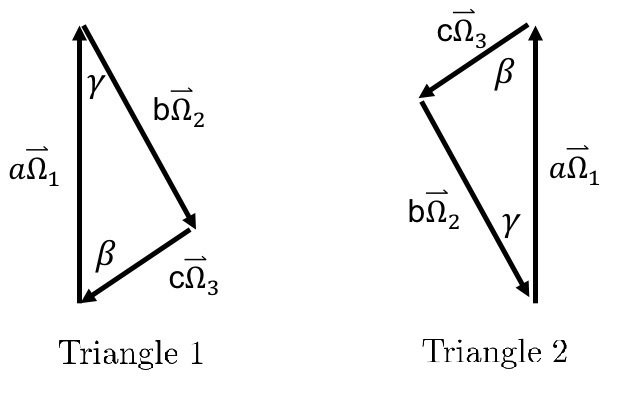
Figure 1: Two types of triangles which satisfy the momentum conservation are depicted. The angles $\beta$ and $\gamma$ are related to $a,b,c$ as $\beta=\mathrm{Arccos}\left(\frac{c^{2}+a^{2}-b^{2}}{2ca}\right)({\rm for}\ c,a\neq 0)$ and $\gamma=\mathrm{Arccos}\left(\frac{a^{2}+b^{2}-c^{2}}{2ab}\right)({\rm for}\ a,b\neq 0)$.

We will carry out the integral about these variables.

On the other hand, the directions of pulsars from the Earth can be defined by

$$\hat{p}_{1}=\left(\begin{array}[]{ccc}0\\ 0\\ 1\end{array}\right),\>\>\>\>\>\hat{p}_{2}=\left(\begin{array}[]{ccc}\cos\xi_{2}\sin\psi_{2}\\ \sin\xi_{2}\sin\psi_{2}\\ \cos\psi_{2}\end{array}\right),\>\>\>\>\>\hat{p}_{3}=\left(\begin{array}[]{ccc}\cos\xi_{3}\sin\psi_{3}\\ \sin\xi_{3}\sin\psi_{3}\\ \cos\psi_{3}\end{array}\right)\ .$$ (29)

Note that we have fixed $\hat{p}_{1}$ to be the $z$-direction. Although one can set $\xi_{3}=0$ without loss of generality, we leave it to keep $\xi_{2}$ and $\xi_{3}$ symmetric for a while.

Below we express $F^{A}(\hat{\Omega}_{i},\hat{p}_{i})$ defined by Eq. (5) in terms of the constants $\gamma,\beta,\xi_{2},\psi_{2},\xi_{3},\psi_{3}$ and the integration variables $\phi,\theta,\Phi$ to carry out the integral (28).

V.1 Computation of Pattern functions

The direction of $\hat{\Omega}_{1}$ is

$$\hat{\Omega}_{1}=R_{z}(\phi)\,R_{y}(\theta)\,\vec{e}_{z}=\left(\begin{array}[]{ccc}\cos\phi\sin\theta\\ \sin\phi\sin\theta\\ \cos\theta\end{array}\right)\,,$$ (30)

where $R_{z}(\phi)$ and $R_{y}(\theta)$ represent the rotation around $z$-axis by $\phi$ and the rotation around $y$-axis by $\theta$, respectively.

To compute $e_{ij}^{A}(\hat{\Omega}_{1})$, it is necessary to determine $\hat{m}(\hat{\Omega}_{1})$ and $\hat{n}(\hat{\Omega}_{1})$. Since any $\hat{m}(\hat{\Omega}_{1})$ and $\hat{n}(\hat{\Omega}_{1})$ are allowed as long as $\hat{m}(\hat{\Omega}_{1})$ and $\hat{n}(\hat{\Omega}_{1})$ are perpendicular to $\hat{\Omega}_{1}$ and one another, we choose the following simple ones:

$$\hat{m}(\hat{\Omega}_{1})=R_{z}(\phi)\,R_{y}(\theta)\,\vec{e}_{x}=\left(\begin{array}[]{ccc}\cos\phi\cos\theta\\ \sin\phi\cos\theta\\ -\sin\theta\end{array}\right),\>\>\>\>\>\hat{n}(\hat{\Omega}_{1})=R_{z}(\phi)\,R_{y}(\theta)\,\vec{e}_{y}=\left(\begin{array}[]{ccc}-\sin\phi\\ \cos\phi\\ 0\end{array}\right).$$ (31)

Then, from Eqs. (2) and (5), the pattern functions for $\hat{\Omega}_{1}$ follow as

$$\begin{cases}F^{+}(\hat{\Omega}_{1},\hat{p}_{1})=\frac{1}{2}(1-\cos\theta)\ ,&\\ F^{\times}(\hat{\Omega}_{1},\hat{p}_{1})=0\ .&\end{cases}$$ (32)

Next we compute $F^{A^{\prime}}(\hat{\Omega}_{2},\hat{p}_{2})$ and $F^{A^{\prime\prime}}(\hat{\Omega}_{3},\hat{p}_{3})$. Let us focus on the Triangle 1 for a while. Then, the zenith angle of $\hat{\Omega}_{2}$ with respect to $\hat{\Omega}_{1}$ is $\pi-\gamma$ and the azimuth angle of $\hat{\Omega}_{2}$ around the $\hat{\Omega}_{1}$ is $\Phi$. Similarly, the zenith angle of $\hat{\Omega}_{3}$ with respect to $\hat{\Omega}_{1}$ is $\pi-\beta$ and the azimuth angle of $\hat{\Omega}_{3}$ around the $\hat{\Omega}_{1}$ is $\Phi+\pi$. Therefore, we have

$$\begin{cases}\hat{\Omega}_{2}=R_{z}(X_{2})\,R_{y}(Y_{2})\vec{e}_{z}=R_{z}(\phi)\,R_{y}(\theta)\,R_{z}(\Phi)\,R_{y}(\pi-\gamma)\,R_{y}(-\theta)\,R_{z}(-\phi)\hat{\Omega}_{1}\ ,&\\ \hat{\Omega}_{3}=R_{z}(X_{3})\,R_{y}(Y_{3})\vec{e}_{z}=R_{z}(\phi)\,R_{y}(\theta)\,R_{z}(\Phi+\pi)\,R_{y}(\pi-\beta)\,R_{y}(-\theta)\,R_{z}(-\phi)\hat{\Omega}_{1}\ ,&\end{cases}$$ (33)

where we have defined the zenith angles $X_{2},X_{3}$ and the azimuth angles $Y_{2},Y_{3}$ with respect to z-axis for later use. More explicitly, they obey the equations

$$\left\{\,\,\begin{aligned} \left(\begin{array}[]{ccc}\cos X_{2}\sin Y_{2}\\ \sin X_{2}\sin Y_{2}\\ \cos Y_{2}\\ \end{array}\right)&=&\left(\begin{array}[]{ccc}\cos\Phi\cos\theta\sin\gamma\cos\phi-\cos\phi\sin\theta\cos\gamma-\sin\gamma\sin\Phi\sin\phi\\ \cos\Phi\cos\theta\sin\gamma\sin\phi-\sin\phi\sin\theta\cos\gamma+\sin\gamma\cos\phi\sin\Phi\\ -\sin\theta\cos\Phi\sin\gamma-\cos\theta\cos\gamma\\ \end{array}\right)\,,\\ \left(\begin{array}[]{ccc}\cos X_{3}\sin Y_{3}\\ \sin X_{3}\sin Y_{3}\\ \cos Y_{3}\\ \end{array}\right)&=&\left(\begin{array}[]{ccc}-\cos\Phi\cos\theta\cos\phi\sin\beta-\cos\phi\sin\theta\cos\beta+\sin\Phi\sin\phi\sin\beta\\ -\cos\Phi\cos\theta\sin\phi\sin\beta-\sin\phi\sin\theta\cos\beta-\cos\phi\sin\Phi\sin\beta\\ \sin\theta\cos\Phi\sin\beta-\cos\theta\cos\beta\\ \end{array}\right)\,.\end{aligned}\right.$$ (34)

We can solve the above equations to obtain

$$Y_{2}=\mathrm{Arccos}\left(-\sin\theta\cos\Phi\sin\gamma-\cos\theta\cos\gamma\right)\ ,$$ (35)

$$X_{2}=\left\{\begin{aligned} 0\>\>\>\>\>\>\>\>\>\>\>\>\>\>\>\>\>\>\>\>\>\>\>\>\>\>\>\>\>\>\>\>\>\>\>\>\>\>\>\>\>\>\>\>(Y_{2}=0,\pi)\\ \,\,\\ \mathrm{Arccos}\left[\cfrac{\cos\Phi\cos\theta\sin\gamma\cos\phi-\cos\phi\sin\theta\cos\gamma-\sin\gamma\sin\Phi\sin\phi}{\sqrt{1-\left(\sin\theta\cos\Phi\sin\gamma+\cos\gamma\cos\theta\right)^{2}}}\right]\\ (\cos\Phi\cos\theta\sin\gamma\sin\phi-\sin\phi\sin\theta\cos\gamma+\sin\gamma\cos\phi\sin\Phi\geq 0)\\ \,\,\\ 2\pi-\mathrm{Arccos}\left[\cfrac{\cos\Phi\cos\theta\sin\gamma\cos\phi-\cos\phi\sin\theta\cos\gamma-\sin\gamma\sin\Phi\sin\phi}{\sqrt{1-\left(\sin\theta\cos\Phi\sin\gamma+\cos\gamma\cos\theta\right)^{2}}}\right]\\ ({\rm otherwise})\end{aligned}\right.$$ (36)

and

$$Y_{3}=\mathrm{Arccos}(\sin\theta\cos\Phi\sin\beta-\cos\theta\cos\beta)\ ,$$ (37)

$$X_{3}=\left\{\begin{aligned} 0\>\>\>\>\>\>\>\>\>\>\>\>\>\>\>\>\>\>\>\>\>\>\>\>\>\>\>\>\>\>\>\>\>\>\>\>\>\>\>\>\>\>\>\>(Y_{3}=0,\pi)\\ \,\,\\ \mathrm{Arccos}\left[\cfrac{-\cos\Phi\cos\theta\cos\phi\sin\beta-\cos\phi\sin\theta\cos\beta+\sin\Phi\sin\phi\sin\beta}{\sqrt{1-\left(\sin\theta\cos\Phi\sin\beta-\cos\theta\cos\beta\right)^{2}}}\right]\\ (-\cos\Phi\cos\theta\sin\phi\sin\beta-\sin\phi\sin\theta\cos\beta-\cos\phi\sin\Phi\sin\beta\geq 0)\\ \,\,\\ 2\pi-\mathrm{Arccos}\left[\cfrac{-\cos\Phi\cos\theta\cos\phi\sin\beta-\cos\phi\sin\theta\cos\beta+\sin\Phi\sin\phi\sin\beta}{\sqrt{1-\left(\sin\theta\cos\Phi\sin\beta-\cos\theta\cos\beta\right)^{2}}}\right]\\ ({\rm otherwise})\end{aligned}\right.$$ (38)

On the other hand, unlike $\hat{\Omega}_{i}$, $\hat{m}(\hat{\Omega}_{i})$ and $\hat{n}(\hat{\Omega}_{i})$ depend on the process of rotation rather than the entire rotation. Therefore, $\hat{m}(\hat{\Omega}_{2}),\hat{n}(\hat{\Omega}_{2}),\hat{m}(\hat{\Omega}_{3})$ and $\hat{n}(\hat{\Omega}_{3})$ have to follow the same rotation process of $\hat{m}(\hat{\Omega}_{1})$ and $\hat{n}(\hat{\Omega}_{1})$. Thus,

$$\left\{\,\,\begin{aligned} \hat{m}(\hat{\Omega}_{2})&=&R_{z}(X_{2})R_{y}(Y_{2})\vec{e}_{x}\\ \hat{n}(\hat{\Omega}_{2})&=&R_{z}(X_{2})R_{y}(Y_{2})\vec{e}_{y}\end{aligned}\right.\ \ \ ,\>\>\>\>\>\>\>\>\>\>\left\{\,\,\begin{aligned} \hat{m}(\hat{\Omega}_{3})&=&R_{z}(X_{3})R_{y}(Y_{3})\vec{e}_{x}\\ \hat{n}(\hat{\Omega}_{3})&=&R_{z}(X_{3})R_{y}(Y_{3})\vec{e}_{y}\end{aligned}\right.\ \ .$$ (39)

Now, we can express $F^{A^{\prime}}(\hat{\Omega}_{2},\hat{p}_{2})$ and $F^{A^{\prime\prime}}(\hat{\Omega}_{3},\hat{p}_{3})$ by the constants $\gamma,\beta,\xi_{2},\psi_{2},\xi_{3},\psi_{3}$ and the integration variables $\phi,\theta,\Phi$ through Eqs. (2), (5), (29), (33) and (35)-(39).

V.2 ORF for ($+++$) and ($+\times\times$) modes

For example, the ORF for (+++) mode is evaluated as

$$\Gamma^{+++}(\gamma,\beta;\hat{p}_{1},\hat{p}_{2},\hat{p}_{3})=-\cfrac{1}{(4\pi)^{2}}\,\int_{0}^{2\pi}{\mathrm{d}}\phi\,\int_{-1}^{1}{\mathrm{d}}\cos\theta\,\int_{0}^{2\pi}{\mathrm{d}}\Phi\,\Big{[}\ f(\gamma,\hat{p}_{2};\beta,\hat{p}_{3})+f(\beta,\hat{p}_{3};\gamma,\hat{p}_{2})\ \Big{]}\ ,$$ (40)

where

$$f(\gamma,\hat{p}_{2};\beta,\hat{p}_{3})=\frac{1}{8}\left(1-\cos\theta\right)\,\prod_{i=2,3}\left[\frac{\left(\hat{p}_{i}\cdot\hat{m}(\hat{\Omega}_{i})\right)^{2}-\left(\hat{p}_{i}\cdot\hat{n}(\hat{\Omega}_{i})\right)^{2}}{1+\hat{p}_{i}\cdot\hat{\Omega}_{i}}\right]\,\,.$$ (41)

In Eq. (40), the first and the second terms in the square bracket are from the Triangle 1 and the Triangle 2 of Fig. 1, respectively. We can not calculate (40) analytically in general. However, in a few special cases, such as the co-aligned pulsars/a single pulsar ($\hat{p}_{1}=\hat{p}_{2}=\hat{p}_{3}$) and the anti-parallel pulsars/two oppositely directed pulsars ($\hat{p}_{1}=-\hat{p}_{2}=-\hat{p}_{3}$), the integral can be solved analytically. The analytical expressions are given in Appendix.B.

Taking a look at Eq. (32), we find that the ORF for ($\times A^{\prime}A^{\prime\prime}$) are all zero. Then, there just remain ($++\times$) and ($+\times\times$) modes. However, we found that the integrand for the ($++\times$) mode is odd function, so that the ORF is zero. This can be interpreted as follows: In calculating the ORF for the three point correlation, we sum over all possible triangles. As shown in Fig. 1, this corresponds to adding parity-inverted triangles. Since the response to cross polarization, namely, $F^{\times}(\hat{\Omega}_{i},\hat{p}_{i})$ ($i=2,3$), has odd parity, the contributions from polarization combinations where cross appears only once should be zero. Consequently, we have only ($+++$) and ($+\times\times$) modes which have nonzero values. In the next section, we will show the several results of the ORF for ($+++$) and ($+\times\times$) modes.

VI ORF for ($+++$) mode

In this section, we evaluate the ORF for $(A,A^{\prime},A^{\prime\prime})=(+,+,+)$ mode while changing parameters $(a,b,c,\hat{p}_{1},\hat{p}_{2},\hat{p}_{3})$. Let us show the dependence of the ORF on pulsar configurations in the squeezed and the equilateral momentum triangles. We have calculated the ORF dependence on $\psi_{2}$ and $\psi_{3}$, for $\xi_{2}=0,\pi/20,2\pi/20,3\pi/20,\ldots,39\pi/20$. The definition of the angles $\xi_{i}$ and $\psi_{i}$ are given in Eq. (29) and we have set $\xi_{3}=0$ without loss of generality. Since it turns out that change in $\xi_{2}$ does not drastically affect the behavior of the ORF, the ORFs for $\xi_{2}=0,\frac{\pi}{2}$ are shown in Figs. 2-5 as illustrative examples.

Consider the squeezed momentum triangle: $\frac{b}{a}=1,\frac{c}{a}\rightarrow 0$. In Figs. 2 and 3, we plotted the ORF for the squeezed momentum triangle. From Figs. 2 and 3, we see extremums are on the four edges, $(\psi_{2},\psi_{3})=(0,0),(0,\pi),(\pi,0),(\pi,\pi)$, and the central point $(\psi_{2},\psi_{3})=(\pi/2,\pi/2)$. In particular, the ORFs are maximized when $(\psi_{2},\psi_{3})=(\pi,0),(\pi,\pi)$, namely,

$$\hat{p}_{1}=-\hat{p}_{2}=\hat{p}_{3}\ ,\>\>\>\>\>\mbox{or}\>\>\>\>\>-\hat{p}_{1}=\hat{p}_{2}=\hat{p}_{3}\ .$$ (42)

Notice that $\hat{p}_{1}=\hat{p}_{2}=-\hat{p}_{3}$ does not have the maximum value since $\hat{p}_{1,2}$ and $\hat{p}_{3}$ are not symmetric due to the choice $a=b,c=0$. We also see quadrupolar signature along with $\psi_{2}$ and $\psi_{3}$ directions. It is analogous to the Hellings-Downs curve.

Next, we consider the equilateral momentum triangle: $\frac{b}{a}=\frac{c}{a}=1$. Figs. 4 and 5 show the ORF for this case. At first sight, Figs. 4 and 5 are similar to the squeezed triangle case, Figs. 2 and 3. In fact, the positions of the extremums are the same. However, Figs. 6 and 7 have maximum points at $(\psi_{2},\psi_{3})=(\pi,0),(\pi,\pi),(\pi,0)$, namely,

$$\hat{p}_{1}=-\hat{p}_{2}=\hat{p}_{3}\ ,\>\>\>\>\>\mbox{or}\>\>\>\>\>-\hat{p}_{1}=\hat{p}_{2}=\hat{p}_{3}\ ,\>\>\>\>\>\mbox{or}\>\>\>\>\>\hat{p}_{1}=\hat{p}_{2}=-\hat{p}_{3}\ .$$ (43)

At these maximum points, there is a permutation symmetry of three pulsars. It is because o$a=b=c$. Quadrupolar signature along with $\psi_{2}$ and $\psi_{3}$ directions appears in Figs. 4 and 5 as well as Figs. 2 and 3. We confirmed that such signature is general for any momentum triangle. Furthermore, ORFs take maximum values at the anti-parallel pulsar configuration for any momentum triangle. Therefore, the anti-parallel pulsar configuration is optimal for the detection of ($+++$) mode of the bispectrum.

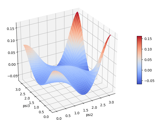
Figure 2: $(-\Gamma^{+++})$ for the squeezed triangle against $\psi_{2}$ and $\psi_{3}$ ($\xi_{2}=0$) is depicted.

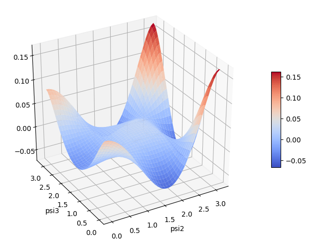
Figure 3: $(-\Gamma^{+++})$ for the squeezed triangle against $\psi_{2}$ and $\psi_{3}$ ($\xi_{2}=\frac{\pi}{2}$) is depicted.

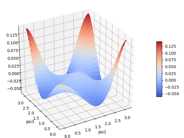
Figure 4: $(-\Gamma^{+++})$ for the equilateral triangle against $\psi_{2}$ and $\psi_{3}$ ($\xi_{2}=0$) is depicted.

Figure 5: $(-\Gamma^{+++})$ for the equilateral triangle against $\psi_{2}$ and $\psi_{3}$ ($\xi_{2}=\frac{\pi}{2}$) is depicted.

VII ORF for ($+\times\times$) mode

As discussed in section V, the ORFs $\Gamma^{AA^{\prime}A^{\prime\prime}}$, are zero other than $\Gamma^{+++}$ and $\Gamma^{+\times\times}$. Thus, in this section, we study $\Gamma^{+\times\times}$. Figs. 6 and 7 show the dependence of the ORF on the pulsar configurations for the squeezed triangle case. Figs. 8 and 9 are for the equilateral triangle case. From Figs. 6-9, one can see that $\Gamma^{+\times\times}$ does not have sensitivity to the co-aligned and the anti-parallel pulsar configurations. Therefore, the co-aligned and the anti-parallel pulsar configurations are suitable to probe $(+++)$ mode of the bispectrum since then only $\Gamma^{+++}$ is non-zero.

On the other hand, we have to choose pulsar configurations other than the co-aligned and the anti-parallel pulsar configurations to probe $(+\times\times)$ mode of the bispectrum. Then one can always find an optimal pulsar configuration corresponding to each momentum triangle. For example, the optimal pulsar configuration for the case of Fig. 6 is $\psi_{2}=2.6,\psi_{3}=2.6$. Potentially, we can separate ($+++$) and ($+\times\times$) modes in (27) with multiple pulsars because $\Gamma^{+++}$ and $\Gamma^{+\times\times}$ are complementary, i.e., positions of peaks are different as depicted in Figs. 2-9.

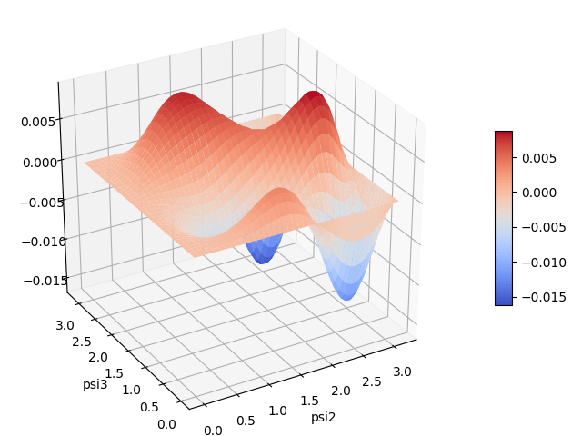
Figure 6: $(-\Gamma^{+\times\times})$ for the squeezed triangle against $\psi_{2}$ and $\psi_{3}$ ($\xi_{2}=0$) is depicted. There is a maximum of the absolute value at $\psi_{2}=2.6,\psi_{3}=2.6$.

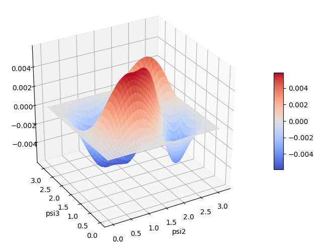
Figure 7: $(-\Gamma^{+\times\times})$ for the squeezed triangle against $\psi_{2}$ and $\psi_{3}$ ($\xi_{2}=\frac{\pi}{2}$) is depicted. There are maximums of the absolute value at $\psi_{2}=1.1,\psi_{3}=0.94$ and $\psi_{2}=1.1,\psi_{3}=2.2$.

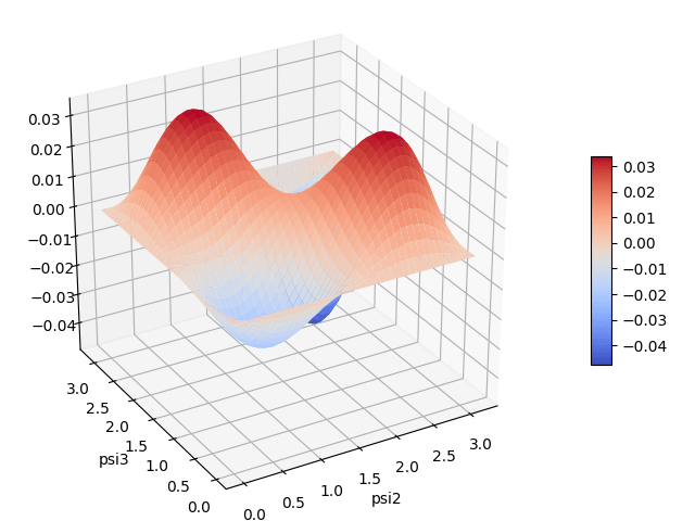
Figure 8: $(-\Gamma^{+\times\times})$ for the equilateral triangle against $\psi_{2}$ and $\psi_{3}$ ($\xi_{2}=0$) is depicted. There is a maximum of the absolute value at $\psi_{2}=2.4,\psi_{3}=2.4$.

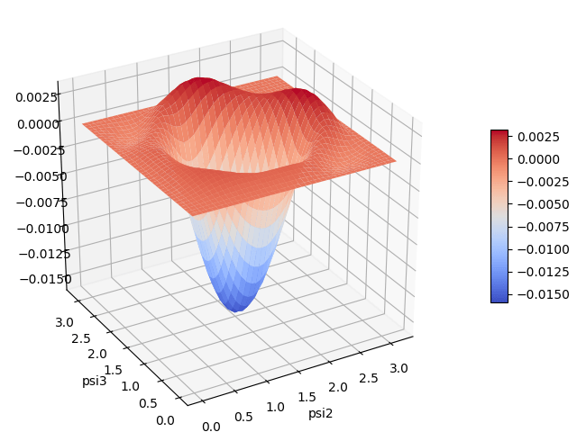
Figure 9: $(-\Gamma^{+\times\times})$ for the equilateral triangle against $\psi_{2}$ and $\psi_{3}$ ($\xi_{2}=\frac{\pi}{2}$) is depicted. There is a maximum of the absolute value at $\psi_{2}=1.5,\psi_{3}=1.5$.

VIII ORF for circular polarization

So far, we have used the linear polarization tensors $e_{ij}^{+}$ and $e_{ij}^{\times}$ as bases of GWs. In this subsection, we investigate the ORF for circular polarization bases defined by

$$e^{{\rm R}}_{ij}(\hat{\Omega})=\frac{e_{ij}^{+}(\hat{\Omega})+ie_{ij}^{\times}(\hat{\Omega})}{\sqrt{2}}\ ,\quad e^{{\rm L}}_{ij}(\hat{\Omega})=\frac{e_{ij}^{+}(\hat{\Omega})-ie_{ij}^{\times}(\hat{\Omega})}{\sqrt{2}}\ .$$ (44)

They then satisfy

$$\left(e^{\sigma}_{ij}(\hat{\Omega})\right)^{*}e^{\sigma^{\prime}}_{ij}(\hat{\Omega})=2\delta^{\sigma\sigma^{\prime}}\ ,\quad\left(e^{{\rm R}}_{ij}(\hat{\Omega})\right)^{*}=e^{{\rm R}}_{ij}(-\hat{\Omega})=e^{{\rm L}}_{ij}(\hat{\Omega})\ ,$$ (45)

where $\sigma,\sigma^{\prime}={\rm R},{\rm L}$. The circular polarization bases are useful to discuss the signature of parity violation Soda:2011am -Bartolo:2017szm . From Eqs. (5), (28) and (44), it is easy to construct the ORF for the circular polarization bases as

$$\begin{cases}\ \Gamma^{{\rm RRR}}=\Gamma^{{\rm RLL}}=\Gamma^{{\rm LLL}}=\Gamma^{{\rm LRR}}=\frac{1}{2\sqrt{2}}\big{[}\Gamma^{+++}-\Gamma^{+\times\times}\big{]}\ ,&\\ \ \Gamma^{{\rm RRL}}=\Gamma^{{\rm RLR}}=\Gamma^{{\rm LLR}}=\Gamma^{{\rm LRL}}=\frac{1}{2\sqrt{2}}\big{[}\Gamma^{+++}+\Gamma^{+\times\times}\big{]}\ .&\end{cases}$$ (46)

They can be evaluated immediately by using the result in previous subsections. Especially, for the case of the co-aligned (or a single pulsar) and the anti-parallel (or two oppositely directed pulsars) configurations, all the ORF for circular polarization bases are given by Eqs. (56) and (57) because then $\Gamma^{+\times\times}$ is zero.

We find that the bispectrum can not be used to detect circular polarization since all the ORFs (LABEL:licir) are parity even and thus all parity violating bispectrum terms such as $\left(B_{{\rm RRR}}-B_{{\rm LLL}}\right)\left(\Gamma^{{\rm RRR}}-\Gamma^{{\rm LLL}}\right)$ are zero. The situation is same for the case of the power spectrum Kato:2015bye . Physically, the three point correlation function is on a plane rather than three-dimensional because we have ignored the pulsar term in Eq. (4), and thus the three point function can not distinguish left and right polarizations. Therefore, one guess that the four point correlation function could detect parity violation with pulsar timing arrays.

IX Conclusion

We explored the possibility of the detection of the bispectrum of stochastic gravitational waves with pulsar timing arrays. We showed that an appropriate filter function in three point correlations enables us to extract a specific configuration of momentum triangles in the bispectrum of stochastic GWs. Therefore, one can probe the bispectral shape, which carries important information of the early universe, by adjusting the filter function.

Furthermore, we considered the three point correlation in pulsar timing measurement and investigated the dependence of the sensitivity, i.e. ORF, on the pulsar configurations and the momentum triangle which we want to probe. Several examples of the result are shown in Figs. 2-9. In ($+++$) mode of the ORF, it was found that the anti-parallel (or two oppositely directed pulsars) configuration universally maximizes the sensitivity of the three point correlation. This is analogous to the ORF for the two point correlation (21) where the configuration for two oppositely directed pulsars has a maximum value. Moreover, as is shown in Figs. 2-5, ($+++$) mode has quadrupolar signature like the Hellings-Downs curve (21). Remarkably, we obtained analytical expressions of the ORF for special cases, (56) and (57). In ($+\times\times$) mode, the ORF does not have the sensitivity in the co-aligned and the anti-parallel pulsar configurations as is depicted in Figs. 6-9. Therefore, the co-aligned and the anti-parallel pulsar configurations are suitable to probe $(+++)$ mode of the bispectrum. Conversely, we have to choose pulsar configurations other than the co-aligned and the anti-parallel pulsar configurations to probe $(+\times\times)$ mode of the bispectrum. Then one can always find an optimal pulsar configuration corresponding to each momentum configuration. Potentially, we can separate ($+++$) and ($+\times\times$) modes in (27) with multiple pulsars because $\Gamma^{+++}$ and $\Gamma^{+\times\times}$ are complementary, i.e., positions of peaks are different as depicted in Figs. 2-9. The ORF for circular polarization bases are also discussed in section VIII and described in Eq. (LABEL:licir). We note that our result, i.e. ORF, is useful for removing noises and increasing the sensitivity with correlation of multiple pulsars Lentati:2015qwp ,Arzoumanian:2018saf .

We roughly estimated the detectable value of the non linear estimator $f_{NL}$ by setting the SNR (54) to be unity, on the assumption that the observation time $T\sim 100$ years and target frequencies $f\sim 3\times 10^{-9}$ Hz, with $100$ pulsars which detectable timing residuals are $\sim 10$ ns. We then got $f_{NL}\sim 10^{12}$.  Then, one may wonder if the non-gaussianity is too small to detect at all Maldacena:2002vr . However, there is another GW source rather than vacuum fluctuations such as particle production during inflation Senatore:2011sp and nonlinear density perturbations after inflation Ananda:2006af . They can produce non-gaussian GWs. For example, vector field production during inflation can induce abundant primordial GWs with large non-gaussianity Cook:2013xea . Non-Abelian gauge fields can also generate very large tensor non-gaussianity because they have a tensor component Agrawal:2017awz . Therefore, the detection of the bispecta is promising.

Appendix A Optimum filter function

In section III and IV, we derived the expression of the two point correlation (17) and the three point correlation (27), respectively. There we left the filter functions $\tilde{Q}(f)$ as an arbitrary function. In this appendix we investigate which form of the filter function $\tilde{Q}(f)$ maximizes the SNR.

To begin with, the variance of $S_{12}$ is defined as

$$\sigma^{2}\equiv\braket{S_{12}^{2}}-\braket{S_{12}}^{2}\,.$$ (47)

Using Eqs. (12) and (13), we obtain

$$\sigma^{2} = \int_{-\infty}^{\infty}\mathrm{d}f\mathrm{d}f^{\prime}\,\tilde{Q}(f)\tilde{Q}(f^{\prime})\times\left[\braket{\tilde{s}_{1}(f)\tilde{s}_{2}(f)\tilde{s}_{1}(f^{\prime})\tilde{s}_{2}(f^{\prime})}-\braket{\tilde{s}_{1}(f)\tilde{s}_{2}(f)}\braket{\tilde{s}_{2}(f^{\prime})\tilde{s}_{1}(f^{\prime})}\right]$$ (48)

$$\simeq \int_{-\infty}^{\infty}{\mathrm{d}}f{\mathrm{d}}f^{\prime}\,\tilde{Q}(f)\tilde{Q}(f^{\prime})\,\braket{\tilde{n}_{1}(f)\tilde{n}_{1}(f^{\prime})}\braket{\tilde{n}_{2}(f)\tilde{n}_{2}(f^{\prime})}\,.$$

where we have assumed $z_{i}\ll n_{i}$. Defining the spectral noise density

$$\braket{\tilde{n}_{i}(f)\tilde{n}_{j}(f^{\prime})}=\cfrac{1}{2}\,\delta(f+f^{\prime})\,\delta_{ij}\,S_{n}^{(i)}(|f|)\ ,$$ (49)

we can rewrite Eq. (48) as

$$\sigma^{2}=\frac{T}{2}\int_{0}^{\infty}\mathrm{d}f\,\tilde{Q}(f)^{2}\,S_{n}^{(1)}(f)S_{n}^{(2)}(f)\,.$$ (50)

The SNR can be defined as $\frac{\braket{S_{12}}}{\sqrt{\sigma^{2}}}$ and then we have

$${\rm SNR}=\cfrac{\sqrt{2T}\,\int_{0}^{\infty}{\mathrm{d}}f\,S_{h}(f)\tilde{Q}(f)\Gamma}{\left(\int_{0}^{\infty}\mathrm{d}f\,\tilde{Q}(f)^{2}\,S_{n}^{(1)}(f)S_{n}^{(2)}(f)\right)^{1/2}}\ .$$ (51)

From Eq. (51), the optimum $\tilde{Q}(f)$ which maximizes the SNR is

$$\tilde{Q}(f)\propto\cfrac{S_{h}(f)}{S_{n}^{(1)}(f)S_{n}^{(2)}(f)}\ .$$ (52)

It is determined by $S_{h}(f)$, $S_{n}^{(1)}(f)$ and $S_{n}^{(2)}(f)$.

Next, we extend above discussion to the case of the three point correlation. One can obtain the variation of $S_{123}$ in the same manner as the two point correlation case:

$$\sigma^{2}=\frac{T^{2}}{4abc}\,\int_{0}^{\infty}\mathrm{d}f\tilde{Q}(f)^{2}S_{n}^{(1)}(af)S_{n}^{(2)}(bf)S_{n}^{(3)}(cf)\ .$$ (53)

Then, the SNR defined by $\frac{\braket{S_{123}}}{\sqrt{\sigma^{2}}}$ is

$${\rm SNR}=\frac{4\sum_{A,A^{\prime},A^{\prime\prime}}\int_{0}^{\infty}\mathrm{d}f\frac{1}{f^{3}}\,B_{AA^{\prime}A^{\prime\prime}}(af,bf,cf)\tilde{Q}(f)\frac{\sin\big{(}\pi(a+b+c)fT\big{)}}{\pi(a+b+c)fT}(4\pi)^{2}\Gamma^{AA^{\prime}A^{\prime\prime}}(a,b,c;\hat{p}_{1},\hat{p}_{2},\hat{p}_{3})}{\left(abc\int_{0}^{\infty}\mathrm{d}f\tilde{Q}(f)^{2}S_{n}^{(1)}(af)S_{n}^{(2)}(bf)S_{n}^{(3)}(cf)\right)^{1/2}}\ .$$ (54)

We get the optimum filter function by requiring it to maximize the SNR as

$$\tilde{Q}(f)\propto\cfrac{\sum_{A,A^{\prime},A^{\prime\prime}}\frac{1}{f^{3}}B_{AA^{\prime}A^{\prime\prime}}(af,bf,cf)\frac{\sin\big{(}\pi(a+b+c)fT\big{)}}{\pi(a+b+c)fT}\Gamma^{AA^{\prime}A^{\prime\prime}}(a,b,c;\hat{p}_{1},\hat{p}_{2},\hat{p}_{3})}{S_{n}^{(1)}(af)S_{n}^{(2)}(bf)S_{n}^{(3)}(cf)}\ .$$ (55)

It is determined by the bispectrum, the ORF and the noises.

Appendix B Analytical expression of ORF for special cases

For the cases of the co-aligned pulsars/a single pulsar ($\hat{p}_{1}=\hat{p}_{2}=\hat{p}_{3}$) and the anti-parallel pulsars/two oppositely directed pulsars ($\hat{p}_{1}=-\hat{p}_{2}=-\hat{p}_{3}$), we can solve the integral (40) analytically. The results are

$$\Gamma^{+++}(\beta,\gamma)=-\frac{1}{24}\big{(}3+\cos(\beta-\gamma)-\cos\beta-\cos\gamma\big{)}\quad({\rm for\ co\mathchar 45\relax aligned})\ ,$$ (56)

$$\Gamma^{+++}(\beta,\gamma)=-\frac{1}{24}\big{(}3+\cos(\beta-\gamma)+\cos\beta+\cos\gamma\big{)}\quad({\rm for\ anti\mathchar 45\relax parallel})\ .$$ (57)

In Eq. (56), there is a peak at $\beta=\gamma=\frac{\pi}{2}$, namely, the squeezed momentum triangle. On the other hand, Eq. (57) has a peak at $\beta=\gamma=0$, namely, the folded momentum triangle. From Eqs. (56) and (57), we see that the ORF for the anti-parallel pulsar configuration is always larger than that for the co-aligned pulsar configuration. We numerically confirmed that the anti-parallel pulsar configuration maximizes the ORF for any momentum triangle. Therefore, the anti-parallel pulsar configuration is optimal for the detection of ($+++$) mode of the bispectrum.

We mention that numerical evaluations of the ORFs corresponded with the analytical solutions (56) and (57). It justifies the numerical calculation of ORFs.

References

- (1) L. P. Grishchuk, Sov. Phys. JETP 40, 409 (1975) [Zh. Eksp. Teor. Fiz. 67, 825 (1974)].
- (2) A. A. Starobinsky, JETP Lett. 30, 682 (1979) [Pisma Zh. Eksp. Teor. Fiz. 30, 719 (1979)].
- (3) A. A. Starobinsky, Phys. Lett. B 91, 99 (1980) [Phys. Lett. 91B, 99 (1980)] [Adv. Ser. Astrophys. Cosmol. 3, 130 (1987)].
- (4) K. Sato, Mon. Not. Roy. Astron. Soc. 195, 467 (1981).
- (5) A. H. Guth, Phys. Rev. D 23, 347 (1981) [Adv. Ser. Astrophys. Cosmol. 3, 139 (1987)].
- (6) A. D. Linde, Phys. Lett. 108B, 389 (1982) [Adv. Ser. Astrophys. Cosmol. 3, 149 (1987)].
- (7) T. Regimbau, Res. Astron. Astrophys. 11, 369 (2011) [arXiv:1101.2762 [astro-ph.CO]].
- (8) D. Coward and T. Regimbau, New Astron. Rev. 50, 461 (2006) [astro-ph/0607043].
- (9) S. Drasco and E. E. Flanagan, Phys. Rev. D 67, 082003 (2003) [gr-qc/0210032].
- (10) D. M. Coward and R. R. Burman, Mon. Not. Roy. Astron. Soc. 361, 362 (2005) [astro-ph/0505181].
- (11) E. Racine and C. Cutler, Phys. Rev. D 76, 124033 (2007) [arXiv:0708.4242 [gr-qc]].
- (12) N. Seto, Astrophys. J. 683, L95 (2008) [arXiv:0807.1151 [astro-ph]].
- (13) N. Seto, Phys. Rev. D 80, 043003 (2009) [arXiv:0908.0228 [gr-qc]].
- (14) E. Thrane, Phys. Rev. D 87, no. 4, 043009 (2013) [arXiv:1301.0263 [astro-ph.IM]].
- (15) D. Baumann, arXiv:0907.5424 [hep-th].
- (16) D. Babich, P. Creminelli and M. Zaldarriaga, JCAP 0408, 009 (2004) [astro-ph/0405356].
- (17) N. Bartolo, E. Komatsu, S. Matarrese and A. Riotto, Phys. Rept. 402, 103 (2004) [astro-ph/0406398].
- (18) G. Goon, K. Hinterbichler, A. Joyce and M. Trodden, arXiv:1812.07571 [hep-th].
- (19) A. Ito and J. Soda, Phys. Lett. B 771, 415 (2017) [arXiv:1607.07062 [hep-th]].
- (20) E. Dimastrogiovanni, M. Fasiello, G. Tasinato and D. Wands, arXiv:1810.08866 [astro-ph.CO].
- (21) R. Saito and T. Kubota, JCAP 1806, no. 06, 009 (2018) [arXiv:1804.06974 [hep-th]].
- (22) X. Chen and Y. Wang, JCAP 1004, 027 (2010) [arXiv:0911.3380 [hep-th]].
- (23) D. Baumann and D. Green, Phys. Rev. D 85, 103520 (2012) [arXiv:1109.0292 [hep-th]].
- (24) T. Noumi, M. Yamaguchi and D. Yokoyama, JHEP 1306, 051 (2013) [arXiv:1211.1624 [hep-th]].
- (25) N. Arkani-Hamed and J. Maldacena, arXiv:1503.08043 [hep-th].
- (26) H. Lee, D. Baumann and G. L. Pimentel, JHEP 1612, 040 (2016) [arXiv:1607.03735 [hep-th]].
- (27) B. P. Abbott et al. [LIGO Scientific and Virgo Collaborations], Phys. Rev. Lett. 118, no. 12, 121101 (2017) Erratum: [Phys. Rev. Lett. 119, no. 2, 029901 (2017)] [arXiv:1612.02029 [gr-qc]].
- (28) J. Abadie et al. [LIGO Scientific and VIRGO Collaborations], Phys. Rev. D 85, 122001 (2012) [arXiv:1112.5004 [gr-qc]].
- (29) L. Lentati et al., Mon. Not. Roy. Astron. Soc. 453, no. 3, 2576 (2015) [arXiv:1504.03692 [astro-ph.CO]].
- (30) Z. Arzoumanian et al. [NANOGRAV Collaboration], Astrophys. J. 859, no. 1, 47 (2018) [arXiv:1801.02617 [astro-ph.HE]].
- (31) P. D. Lasky et al., Phys. Rev. X 6, no. 1, 011035 (2016) doi:10.1103/PhysRevX.6.011035 [arXiv:1511.05994 [astro-ph.CO]].
- (32) N. Bartolo et al., JCAP 1612, no. 12, 026 (2016) [arXiv:1610.06481 [astro-ph.CO]].
- (33) S. Sato et al., J. Phys. Conf. Ser. 840, no. 1, 012010 (2017).
- (34) G. Janssen et al., PoS AASKA 14, 037 (2015) [arXiv:1501.00127 [astro-ph.IM]].
- (35) W. Zhao, Y. Zhang, X. P. You and Z. H. Zhu, Phys. Rev. D 87, no. 12, 124012 (2013) doi:10.1103/PhysRevD.87.124012 [arXiv:1303.6718 [astro-ph.CO]].
- (36) B. Allen and J. D. Romano, Phys. Rev. D 59, 102001 (1999) [gr-qc/9710117].
- (37) M. Maggiore, Phys. Rept. 331, 283 (2000) [gr-qc/9909001].
- (38) J. D. Romano and N. J. Cornish, Living Rev. Rel. 20, no. 1, 2 (2017) [arXiv:1608.06889 [gr-qc]].
- (39) R. w. Hellings and G. s. Downs, Astrophys. J. 265, L39 (1983).
- (40) M. Anholm, S. Ballmer, J. D. E. Creighton, L. R. Price and X. Siemens, Phys. Rev. D 79, 084030 (2009) [arXiv:0809.0701 [gr-qc]].
- (41) N. Bartolo et al., arXiv:1806.02819 [astro-ph.CO].
- (42) N. Bartolo, V. De Luca, G. Franciolini, M. Peloso and A. Riotto, arXiv:1810.12218 [astro-ph.CO].
- (43) N. Bartolo, V. De Luca, G. Franciolini, M. Peloso, D. Racco and A. Riotto, arXiv:1810.12224 [astro-ph.CO].
- (44) J. Soda, H. Kodama and M. Nozawa, JHEP 1108, 067 (2011) [arXiv:1106.3228 [hep-th]].
- (45) I. Obata and J. Soda, Phys. Rev. D 93, no. 12, 123502 (2016) Addendum: [Phys. Rev. D 95, no. 10, 109903 (2017)] [arXiv:1602.06024 [hep-th]].
- (46) I. Obata and J. Soda, Phys. Rev. D 94, no. 4, 044062 (2016) [arXiv:1607.01847 [astro-ph.CO]].
- (47) M. Satoh, S. Kanno and J. Soda, Phys. Rev. D 77, 023526 (2008) [arXiv:0706.3585 [astro-ph]].
- (48) T. Takahashi and J. Soda, Phys. Rev. Lett. 102, 231301 (2009) [arXiv:0904.0554 [hep-th]].
- (49) T. Zhu, W. Zhao, Y. Huang, A. Wang and Q. Wu, Phys. Rev. D 88, 063508 (2013) [arXiv:1305.0600 [hep-th]].
- (50) N. Bartolo and G. Orlando, JCAP 1707, 034 (2017)
- (51) R. Kato and J. Soda, Phys. Rev. D 93, no. 6, 062003 (2016) [arXiv:1512.09139 [gr-qc]].
- (52) J. M. Maldacena, JHEP 0305, 013 (2003) [astro-ph/0210603].
- (53) L. Senatore, E. Silverstein and M. Zaldarriaga, JCAP 1408, 016 (2014) [arXiv:1109.0542 [hep-th]].
- (54) K. N. Ananda, C. Clarkson and D. Wands, Phys. Rev. D 75, 123518 (2007) [gr-qc/0612013].
- (55) J. L. Cook and L. Sorbo, JCAP 1311, 047 (2013) [arXiv:1307.7077 [astro-ph.CO]].
- (56) A. Agrawal, T. Fujita and E. Komatsu, Phys. Rev. D 97, no. 10, 103526 (2018) [arXiv:1707.03023 [astro-ph.CO]].
- (57) A. Lewis: private communication.