Abstract

Parameter reduction has been an important topic in deep learning due to the ever-increasing size of deep neural network models and the need to train and run them on resource limited machines. Despite many efforts in this area, there were no rigorous theoretical guarantees on why existing neural net compression methods should work. In this paper, we provide provable guarantees on some hashing-based parameter reduction methods in neural nets. First, we introduce a neural net compression scheme based on random linear sketching (which is usually implemented efficiently via hashing), and show that the sketched (smaller) network is able to approximate the original network on all input data coming from any smooth and well-conditioned low-dimensional manifold. The sketched network can also be trained directly via back-propagation. Next, we study the previously proposed HashedNets architecture and show that the optimization landscape of one-hidden-layer HashedNets has a local strong convexity property similar to a normal fully connected neural network. We complement our theoretical results with empirical verifications.

 

Towards a Theoretical Understanding of Hashing-Based Neural Nets

 

Yibo Lin yibolin@utexas.edu                        Zhao Song zhaos@g.harvard.edu                        Lin F. Yang lin.yang@princeton.edu UT-Austin                        Harvard & UT-Austin                        Princeton University

1 Introduction

In the past decade, deep neural networks have become the new standards for many machine learning applications, including computer vision Krizhevsky et al. (2012); He et al. (2016), natural language processing Zaremba et al. (2014); Gehring et al. (2017), speech recognition Graves et al. (2013); Amodei et al. (2016), robotics Lillicrap et al. (2015), game playing Silver et al. (2016, 2017), etc. Such model usually contains an enormous number of parameters, which is often much larger than the number of available training samples. Therefore, these networks are usually trained on modern computer clusters which have a huge amount of memory and computation power. On the other hand, there is an increasing need to train and run personalized machine learning models on mobile and embedded devices instead of transferring mobile data to a remote computation center on which all the computations are performed. This is because real-time processing of deep learning models on mobile devices brings the benefits of better privacy and less Internet bandwidth. However, mobile devices like smart phones do not have the memory or computation capability of training large neural networks or even storing these models.

These trends motivate the study of neural network compression, with the goal of reducing the memory overhead required to train, store and run neural networks. There is a recent line of research in this direction, for example Chen et al. (2015); Iandola et al. (2016); Han et al. (2016). Despite their empirical effectiveness, there is little theoretical understanding on why these methods perform well.

The goal of this paper is to bridge the gap between theory and practice in neural network compression. Our focus is on hashing-based methods, which have been studied empirically in e.g. Chen et al. (2015, 2016), with the hope that the randomness in hash functions helps preserve the properties of neural networks despite a reduction in the number of effective parameters. We make this intuition formal by giving theoretical guarantees on the approximation power and the parameter recovery of such networks.

First, we propose a neural net compression scheme based on random linear sketching, which can be efficiently implemented using a hash function. Similar idea has been proposed in Kasiviswanathan et al. (2017) and demonstrated high performance empirically, but no formal theoretical guarantee was known. We show that such compression has strong approximation power. Namely, the small network obtained after sketching can approximate the original network on all input data coming from any low-dimensional manifold with some regularity properties. The sketched network is also directly trainable via back-propagation. In fact, sketching is a principled technique for dimensionality reduction, which has been shown to be very powerful in solving various problems arising in statistics Raskutti and Mahoney (2016); Wang et al. (2017) and numerical linear algebra Woodruff (2014). Given its theoretical success, it is natural to ask whether sketching can be applied to the context of neural net compression with theoretical guarantees. Our result makes partial progresses on this question.

Next we study HashedNets, a simple method proposed in Chen et al. (2015) which appears to perform well in practice. HashedNets directly applies a random hash function on the connection weights in a neural net and to enforce all the weights mapped to the same hash bucket to take the same value. In this way the number of trainable parameters is reduced to be the number of different hash buckets, and training can still be performed via back-propagation while taking the weight sharing structure into account. From the perspective of optimization, we show that the training objective for a one-hidden-layer hashed neural net has a local strong convexity property, similar to that of a normal fully connected network Zhong et al. (2017b). Additionally, we can apply the initialization algorithm in Zhong et al. (2017b) to obtain a good initialization for training. Therefore it implies that the parameters in one-hidden-layer HashedNets can be provably recovered under milde assumptions.

Below we describe our contributions in more detail.

Approximation Power

Our result on the approximation power of sketched nets is based on a classical concept, “subspace embedding”, which originally appears in numerical linear algebra Sarlós (2006). Roughly speaking, it says that there exist a wide family of random matrices $S\in\mathbb{R}^{s\times n}$, such that for any $d$-dimensional subspace $\mathcal{U}\subset\mathbb{R}^{n}$, with probability $1-\delta$ we have $\left\langle Sx,Sx^{\prime}\right\rangle=\langle x,x^{\prime}\rangle\pm\epsilon\|x\|_{2}\|x^{\prime}\|_{2}$ for all $x,x^{\prime}\in\mathcal{U}$, provided $s=\Omega\left(\left(d+\log 1/\delta\right)/\epsilon^{2}\right)$. This result means that the inner product between every two points in a subspace can be approximated simultaneously after applying a random sketching matrix $S$, which is interesting if $s\ll n$. There has been a line of work trying to do subspace embedding using different sketching matrices (e.g. Nelson and Nguyên (2013); Cohen (2016)). Sparse matrices are of particular interests, since for a sparse matrix $S$, one can compute $Sx$ more efficiently. For example, Nelson and Nguyên (2013) showed that it is possible to construct $S$ with only $\widetilde{O}(1/\epsilon)$ nonzero entries per column, which significantly improves the trivial upper bound $\widetilde{O}(d/\epsilon^{2})$. Furthermore, many of these sketching matrices can be efficiently implemented by $k$-wise independent hash functions where $k$ is very small, which only takes a small amount of space to store, and multiplying $S$ with a vector can be computed efficiently.

We extend the idea of subspace embedding to deep learning and show that a feed-forward fully connected network with Lipschitz-continuous activation functions can be approximated using random sketching on all input data coming from a low-dimensional subspace. Below we describe our result for one-hidden-layer neural nets, and this can be generalized to multiple layers.

Consider a one-hidden-layer neural net with input dimension $n$ and $k$ hidden nodes. It can be parameterized by a weight matrix $W\in\mathbb{R}^{n\times k}$ and a weight vector $v\in\mathbb{R}^{k}$, and the function this network computes is $x\mapsto v^{\top}\phi(W^{\top}x)$, where $x\in\mathbb{R}^{n}$ is the input, and $\phi$ should be viewed as a nonlinear activation function acting coordinate-wise on a vector. Our result says that under appropriate assumptions, one can choose a random sketching matrix $S\in\mathbb{R}^{s\times n}$, such that for any $d$-dimensional subspace $\mathcal{U}\subset\mathbb{R}^{n}$, we have

$$\left|v^{\top}\phi(W^{\top}x)-v^{\top}\phi(W^{\top}S^{\top}Sx)\right|\leq\epsilon,\forall x\in\mathcal{U},\|x\|_{2}\leq 1.$$

This result essentially says that the weight matrix $W^{\top}$ can be replaced by $W^{\top}S^{\top}S$, which has rank $s$. When $s<n$, this means that the effective number of parameters can be reduced from $kn$ to $ks$. As we mentioned, the sketching matrix $S$ can be implemented by hash functions in small space and multiplying it with a vector is efficient. The sketched network is also directly trainable, because we can train the $s\times k$ matrix $\widehat{W}=SW$, regarding another factor $S$ in the decomposition $W^{\top}S^{\top}S=\widehat{W}S$ as a known layer.

This result can be generalized to multi-layer neural nets, and we present the details in Section 3. We also note that our result can be easily generalized to low-dimensional manifolds under some regularity condition (see Definition 2.3 in Baraniuk and Wakin (2009)), which is a much more realistic assumption on data.

Parameter Recovery.

It is known that training a neural net is NP-hard in the worst case, even if it only has $3$ hidden nodes Blum and Rivest (1993). Recently, there has been some theoretical progress on understanding the optimization landscapes of shallow neural nets under special input distributions. In particular, Zhong et al. (2017b) gave a recovery guarantee for one-hidden-layer neural nets. They showed that if the input distribution is Gaussian and the ground-truth weight vectors corresponding to hidden nodes are linearly independent, then the true parameters can be recovered in polynomial time given finite samples. This was proved by showing that the training objective is locally strongly convex and smooth around the ground-truth point, together with an initialization method that can output a point inside the locally “nice” region. In this work, we show that local strong convexity and smoothness continue to hold if we replace the fully connected network by HashedNets which has a weight sharing structure enforced by a hash function. We present this result in Section 4.

1.1 Related Works

Parameter Reduction in Deep Learning.

There has been a series of empirical works on reducing the number of free parameters in deep neural networks: Denil et al. (2013) show a method to learn low-rank decompositions of weight matrices in each layer, Chen et al. (2015) propose an approach to use a hash function to enforce parameter sharing, Cheng et al. (2015) adopt a circulant matrix structure for parameter reduction, Sindhwani et al. (2015) study a more general class of structured matrices for parameter reduction.

Sketching and Neural Networks.

Daniely et al. (2016) show that any linear or sparse polynomial function on sparse binary data can be computed by a small single-layer neural net on a linear sketch of the data. Kasiviswanathan et al. (2017) apply a random sketching on weight matrices/tensors, but they only prove that given a fixed layer input, the output of this layer using sketching matrices is an unbiased estimator of the original output of this layer and has bounded variance; however, this does not provide guarantees on the approximation power of the whole sketching-based deep net.

Subspace Embedding.

Subspace embedding Sarlós (2006) is a fundamental tool for solving numerical linear algebra problems, e.g. linear regression, matrix low-rank approximation Clarkson and Woodruff (2013); Nelson and Nguyên (2013); Razenshteyn et al. (2016); Song et al. (2017b), tensor low-rank approximation Song et al. (2019). See also Woodruff (2014) for a survey on this topic.

Recovery Guarantee of Neural Networks.

Since learning a neural net is NP-hard in the worst case Blum and Rivest (1993), many attempts have been made to design algorithms that learns a neural net provably in polynomial time and sample complexity under additional assumptions, e.g., Sedghi and Anandkumar (2014); Zhang et al. (2015); Janzamin et al. (2015); Goel et al. (2017); Goel and Klivans (2017a, b). Another line of work focused on analyzing (stochastic) gradient descent on shallow networks for Gaussian input distributions, e.g., Brutzkus and Globerson (2017); Zhong et al. (2017a, b); Tian (2017); Li and Yuan (2017); Du et al. (2017); Soltanolkotabi (2017).

Other Related Works

Instead of understanding the parameter reduction as our work, there are several results working on developing over-parameterization theory of deep ReLU neural networks, e.g. Allen-Zhu et al. (2018a, b). Thirty years ago, Blum and Rivest proved training neural network is NP-hard Blum and Rivest (1993). Later, neural networks have been shown hard in several different perspectives Klivans and Sherstov (2009); Livni et al. (2014); Daniely (2016); Daniely and Shalev-Shwartz (2016); Goel et al. (2017); Song et al. (2017a); Katz et al. (2017); Weng et al. (2018); Manurangsi and Reichman (2018) in the worst case regime.

Arora et al. proved a stronger generalization for deep nets via a compression approach Arora et al. (2018). There is a long line of works targeting on explaining GAN from theoretical perspective Arora and Zhang (2017); Arora et al. (2017b, a); Bora et al. (2017); Li et al. (2018); Santurkar et al. (2018); Van Veen et al. (2018); Xiao et al. (2018). There is also a long line of provable results about adversarial examples Madry et al. (2017); Bubeck et al. (2018b, a); Weng et al. (2018); Schmidt et al. (2018); Tran et al. (2018).

2 Preliminaries

For any positive integer $n$, we use $[n]$ to denote the set $\{1,2,\cdots,n\}$. Let $a\pm b$ represent any number in the interval $[a-b,a+b]$. For any vector $x\in\mathbb{R}^{n}$, we use $\|x\|_{2}$, $\|x\|_{1}$ and $\|x\|_{\infty}$ to denote its $\ell_{2}$, $\ell_{1}$ and $\ell_{\infty}$ norms, respectively. For $x,y\in\mathbb{R}^{n}$, we use $\langle x,y\rangle$ to denote the standard Euclidean inner product $x^{\top}y$.

For a matrix $A$, let $\det(A)$ denote its determinant (if $A$ is a square matrix), let $A^{\dagger}$ denote the Moore-Penrose pseudoinverse of $A$, and let $\|A\|_{F}$ and $\|A\|_{2}$ denote respectively the Frobenius norm and the spectral norm of $A$. Denote by $\sigma_{i}(A)$ the $i$-th largest singular value of $A$. We use $\operatorname{nnz}(A)$ to denote the number of non-zero entries in $A$.

For any function $f$, we define $\widetilde{O}(f)$ to be $f\cdot\log^{O(1)}(f)$. In addition to $O(\cdot)$ notation, for two functions $f,g$, we use the shorthand $f\lesssim g$ (resp. $\gtrsim$) to indicate that $f\leq Cg$ (resp. $\geq$) for an absolute constant $C$. We use $f\eqsim g$ to mean $cf\leq g\leq Cf$ for constants $c,C$.

We define the $\ell_{1}$ and $\ell_{2}$ balls in $\mathbb{R}^{n}$ as: ${\cal B}_{1}(B,n)=\{x\in\mathbb{R}^{n}\leavevmode\nobreak\ |\leavevmode\nobreak\ \|x\|_{1}\leq B\},{\cal B}_{2}(B,n)=\{x\in\mathbb{R}^{n}\leavevmode\nobreak\ |\leavevmode\nobreak\ \|x\|_{2}\leq B\}.$ We also need the definitions of Lipschitz-continuous functions and $k$-wise independent hash families.

Definition 2.1.

A function $f:\mathbb{R}\rightarrow\mathbb{R}$ is $L$-Lipshitz continuous, if for all $x_{1},x_{2}\in\mathbb{R}$, $|f(x_{1})-f(x_{2})|\leq L|x_{1}-x_{2}|.$

Definition 2.2.

A family of hash functions ${\cal H}\subseteq\{h\mid h:U\to[B]\}$ is said to be $k$-wise independent if for any $x_{1},\ldots,x_{k}\in U$ and any $y_{1},\ldots,y_{k}\in[B]$ we have $\Pr_{h\sim{\cal H}}[h(x_{i})=y_{i},\forall i\in[k]]=\frac{1}{B^{k}}.$

3 The Approximation Power of Parameter-Reduced Neural Networks

In this section, we study the approximation power of parameter-reduced neural nets based on hashing. Any weight matrix $W$ in a neural net acts on a vector $x$ as $Wx$. We replace $Wx$ by $WS^{\top}Sx$ for some sketching ($\#$rows $<$ $\#$columns) matrix $S$ defined in the following section. Then the new weight matrix $WS^{\top}$ has much fewer parameters. We show that if $S$ is chosen properly as a subspace embedding (formally defined later in this section), the sketched network can approximate the original network on all inputs coming from a low-dimensional subspace or manifold. Our sketching matrix is chosen as a Johnson-Lindenstrauss (JL) Johnson and Lindenstrauss (1984) transformation matrix. In Section 3.1, we provide some preliminaries on subspace embedding. In Sections 3.2 and 3.3, we present our result on one-hidden-layer neural nets. Then in Section 3.4 we extend this result to multi-layer neural nets and show a similar approximation guarantee. This provides a theoretical guarantee for hashing-based parameter-reduced networks used in practice.

3.1 Subspace Embedding

We first present some basic definitions of sketching and subspace embedding. These mathematical tools are building blocks for us to understand parameter-reduced neural networks.

Definition 3.1 (Subspace Embedding).

A $(1\pm\epsilon)$ $\ell_{2}$-subspace embedding for the column space of an $n\times d$ matrix $U$ is a matrix $S$ for which for all $x\in\mathrm{colspan}(U)$, $\|Sx\|_{2}^{2}=(1\pm\epsilon)\|x\|_{2}^{2},$or equivalently, for all $x,x^{\prime}\in\mathrm{colspan}(U)$, $\langle Sx,Sx^{\prime}\rangle=\langle x,x^{\prime}\rangle\pm\epsilon\|x\|_{2}\|x^{\prime}\|_{2}.$

Constructions of subspace embedding can be found in e.g. Nelson and Nguyên (2013) from which there is the following theorem.

Theorem 3.2 (Nelson and Nguyên (2013)).

There is a $(1\pm\epsilon)$ oblivious $\ell_{2}$-subspace embedding for $n\times d$ matrix $U$ with $s=d\cdot\operatorname{poly}\log(d/(\epsilon\delta))/\epsilon^{2}$ rows and error probability $\delta$. Further, $S\cdot U$ can be computed in time $O(\operatorname{nnz}(U)\operatorname{poly}\log(d/(\epsilon\delta))/\epsilon)$. We call $S$ a SparseEmbedding matrix.

There are also other subspace embedding matrices, e.g., CountSketch. We provide additional definitions and examples in Section B.1.

Remark 3.3.

We remark that the subspace embedding in Definition 3.1 naturally extends to low dimensional manifolds. For example, for a $d$-dimensional Riemannian submanifold of $\mathbb{R}^{n}$ with volumn $V$ and geodesic covering regularity $R$ (see Definition 2.3 in Baraniuk and Wakin (2009)), Theorem 3.2 holds by replacing $d$ with $Rd\log(V)$. For ease of presentation, we only present our results for subspaces. All our results can be extended to low-dimensional manifolds satisfying regularity conditions.

3.2 One Hidden Layer - Part i@

We consider one-hidden-layer neural nets in the form $\sum_{i}v_{i}\phi_{i}(w_{i}^{\top}x)$, where $x$ is the input vector, $w_{i}$ is a weight vector, $v_{i}$ is a weight scalar, and $\phi_{i}:\mathbb{R}\to\mathbb{R}$ is a nonlinear activation function. In this subsection, we show how to sketch the weights between the input layer and the hidden layer with guaranteed approximation power. The main result is Theorem 3.4 and its proofs are in Appendix B.

Theorem 3.4.

Given parameters $n_{2}\geq 1,n_{1}\geq 1,\epsilon\in(0,1),\delta\in(0,1)$ and $n=\max(n_{2},n_{1})$. Given $n_{2}$ activation functions $\phi_{i}:\mathbb{R}\rightarrow\mathbb{R}$ that are $L$-Lipshitz-continuous, a fixed matrix $U\in\mathbb{R}^{n_{1}\times d}$, weight matrix $W\in\mathbb{R}^{n_{1}\times n_{2}}$ with $\|W\|_{2}\leq B$, $v\in\mathbb{R}^{n_{2}}$ with $\|v\|_{1}\leq B$. Choose a SparseEmbedding matrix $S\in\mathbb{R}^{s\times n_{1}}$ with $s=O(dL^{2}B^{4}A^{2}\epsilon^{-2}\operatorname{poly}\log(nLBA/(\epsilon\delta)))$, then with probability $1-\delta$, we have : for all $x\in\mathrm{colspan}(U)\cap{\cal B}_{2}(A,n_{1})$,

$$|\langle v,\phi(W^{\top}x)\rangle-\langle v,\phi(W^{\top}S^{\top}Sx)\rangle|\leq\epsilon.$$

3.3 One-hidden layer - Part ii@

In this section, we show the approximation power of the compressed network if the weight matrices of both the input layer and output layer are sketched. One of the core idea in the proof is a recursive $\epsilon$-net argument, which plays a crucial role in extending the result to multiple hidden layer. The goal of this section is to prove the following theorem and present the recursive $\epsilon$-net argument.

Theorem 3.5.

Given parameters $n_{2}\geq 1,n_{2}\geq 1,\epsilon\in(0,1),\delta\in(0,1)$ and $n=\max(n_{2},n_{1})$. Given $n_{2}$ activation functions $\phi_{i}:\mathbb{R}\rightarrow\mathbb{R}$ with $L$-Lipshitz and normalized by $1/\sqrt{n_{2}}$, a fixed matrix $U\in\mathbb{R}^{n_{1}\times d}$, and weight matrix $W\in\mathbb{R}^{n_{2}\times n_{1}}$ with $\|W\|_{2}\leq B$, $v\in\mathbb{R}^{n_{2}}$ with $\|v\|_{2}\leq B$. Choose a SparseEmbedding matrix $S_{1}\in\mathbb{R}^{s_{1}\times n_{1}}$ and $S_{2}\in\mathbb{R}^{s_{2}\times n_{2}}$ with $s_{1},s_{2}=O(dL^{2}B^{4}A^{2}\epsilon^{-2}\operatorname{poly}\log(nLBA/(\epsilon\delta)))$, then with probability $1-\delta$, we have : for all $x\in\mathrm{colspan}(U)\cap{\cal B}_{2}(A,n_{1})$,

$$\left|\langle v,\phi(W^{\top}x)\rangle-\langle S_{2}v,S_{2}\phi(W^{\top}S_{1}^{\top}S_{1}x)\rangle\right|\leq\epsilon.$$

The high level idea is as follows. Firstly, we prove that for any fixed input $x$, the theorem statement holds with high probability. Then we build an sufficiently fine $\epsilon$-net over the input space of $x$ and argue that our statement holds for every input point $x$ from the $\epsilon$-net. Condition on this event, the statement holds by applying the Lipshitz continuity of the activation function. The detailed proof is presented in Appendix B.

3.4 Multiple hidden layer

In this section, we generalize our approximation power result to a multi-layer neural network and delay the proofs to Appendix B. Inspired by the batch normalization Ioffe and Szegedy (2015), which has been widely used in practice, we make an additional assumption by requiring the activations to be normalized by $1/\sqrt{n_{j+1}}$ at each layer $j$. The way we deal with multiple hidden layers is, first recursively argue an $\epsilon$-net can be constructed for all the layers with the same size. Then we use triangle inequality to split error into $q+1$ terms and bounding them separately. The result is the following theorem.

Theorem 3.6.

Given parameters $q\geq 1$, $n_{j}\geq 1,\forall j\in[q+1],\epsilon\in(0,1),\delta\in(0,1)$ and $n=\max_{j\in[q+1]}n_{j}$. For each $j\in[q]$, for each $i\in[n_{j+1}]$ let $\phi_{j,i}:\mathbb{R}\rightarrow\mathbb{R}$ denote an activation function with $L$-Lipshitz and normalized by $1/\sqrt{n_{j+1}}$. Given a fixed matrix $U\in\mathbb{R}^{n_{1}\times d}$, $q$ weight matrices $W_{j}\in\mathbb{R}^{n_{j+1}\times n_{j}},\forall j\in[q]$ with (the $i_{j}$-th column of $W_{j}$) $w_{j,i_{j}}\in{\cal B}_{2}(B,n_{j})$, a weight vector $v\in\mathbb{R}^{n_{j+1}}$ with $v\in{\cal B}_{2}(B,n_{j+1})$. For each $j\in[q+1]$, we choose a SparseEmbedding matrix $S_{j}\in\mathbb{R}^{s_{j}\times n_{j}}$ with

$$s_{j}=O(dq^{2}L^{2q}B^{2q+2}A^{2}\epsilon^{-2}\operatorname{poly}\log(nqLBA/(\epsilon\delta))).$$

Then with probability $1-\delta$, we have : for all $x\in\mathrm{colspan}(U)\cap{\cal B}_{2}(A,n_{1})$,

$$|\langle v,f^{(q)}(x)\rangle-\langle S_{q+1}v,S_{q+1}\widetilde{f}^{(q)}(x)\rangle|\leq\epsilon,$$

where $f^{(q)}(x)$ and $\widetilde{f}^{(q)}(x)$ are defined inductively. The base case is $f^{(0)}(x)=\widetilde{f}^{(0)}(x)=x,$ and the inductive case is

$$f^{(j)}(x) =\phi_{j}(W_{j}^{\top}f^{(j-1)}(x)),\forall j\in[q]$$

$$\mathrm{\leavevmode\nobreak\ and\leavevmode\nobreak\ }\widetilde{f}^{(j)}(x) =\phi_{j}(W_{j}^{\top}S_{j}^{\top}S_{j}\widetilde{f}^{(j-1)}(x)),\forall j\in[q].$$

Note that similar results also hold for the case without using $S_{q+1}$. In other words, we only choose $q$ matrices for $q$ hidden layers.

4 Recovery Guarantee

In this section, we study the recovery guarantee of parameter-reduced neural nets. In particular, we study whether (stochastic) gradient descent can learn the true parameters in a one-hidden-layer HashedNets when starting from a sufficiently good initialization point, under appropriate assumptions. We show that even under the special weight sharing structure depicted by the hash function, the resulting neural net still has sufficiently nice properties - namely, local strong convexity and smoothness around the minimizer. Our proof technique is by reducing our case to that of the fully connected network studied in Zhong et al. (2017b). After that, the recovery guarantee follows similarly. We present our result here and give the detailed proof in Appendix C.

We consider the following regression problem : given a set of $m$ samples $S=\{(x_{1},y_{1}),(x_{2},y_{2}),\cdots,(x_{m},y_{m})\}\subset\mathbb{R}^{n}\times\mathbb{R}.$ Let ${\cal D}$ be an underlying distribution over $\mathbb{R}^{n}\times\mathbb{R}$ with parameters $w^{*}\in\mathbb{R}^{B}$ and $v^{*}\in\mathbb{R}^{k}$, such that each sample $(x,y)\in S$ is sampled i.i.d. from this distribution, with $x\sim{\cal N}(0,I),y=\sum_{i=1}^{k}v_{i}^{*}\cdot\phi(\sum_{j=1}^{n}w_{h(i,j)}^{*}\cdot x_{j}).$ Here $h:[k]\times[n]\rightarrow[B]$ is a random hash function drawn from a $t$-wise independent hash family ${\cal H}$, where $t=\Theta(\log(nk))$, and $\phi$ is an activation function.

Note that $w^{*}$ has a corresponding matrix $\widehat{W}^{*}\in\mathbb{R}^{k\times n}$ defined as $\widehat{W}^{*}_{ij}=w^{*}_{h(i,j)}$, which is the actual weight matrix in the HashedNets with a weight sharing structure.

Our goal is to recover the ground-truth parameters $w^{*},v^{*}$ given the sample $S$. Note that how to recover $v^{*}$ has been discussed in Zhong et al. (2017a, b); their method also applies to our situation. Therefore we focus on recovering $w^{*}$ in this section, assuming $v^{*}$ is known.

For a given weight vector $w\in\mathbb{R}^{B}$, we define its expected risk and empirical risk as

$$F_{\cal D}(w) =\frac{1}{2}\operatorname*{{\bf{E}}}_{(x,y)\sim{\cal D}}\left[\left(\sum_{i=1}^{k}v_{i}^{*}\cdot\phi\left(\sum_{j=1}^{n}w_{h(i,j)}\cdot x_{j}\right)-y\right)^{2}\right],$$

$$F_{S}(w) =\frac{1}{2}\sum_{(x,y)\sim S}\left[\left(\sum_{i=1}^{k}v_{i}^{*}\cdot\phi\left(\sum_{j=1}^{n}w_{h(i,j)}\cdot x_{j}\right)-y\right)^{2}\right].$$

We first show a structural result for $t$-wise independent hash family, which says the pre-image of each bucket is pretty balanced.

Lemma 4.1 (Concentration of hashing buckets, part of Lemma C.12).

Given integers $N$ and $B\lesssim N/\log N$. Let $h:[N]\rightarrow[B]$ denote a $t$-wise independent hash function such that $\Pr_{h\sim{\cal H}}[h(i)=j]=1/B,\forall i\in[N],\forall j\in[B].$ Then, if $t=\Theta(\log N)$, with probability at least $1-1/\operatorname{poly}(N)$, we have for all $j\in[B]$, $0.9N/B\leq\sum_{i=1}^{N}{\bf 1}_{h(i)=j}\leq 1.1N/B.$

The previous work Zhong et al. (2017b) showed that a fully connected network whose ground-truth weight matrix $W^{*}\in\mathbb{R}^{k\times n}$ has rank $k$ has local strong convexity and smoothness around $W^{*}$ in its loss function (see their Lemma D.3).

Using Lemma 4.1 as our core reduction tool, we can reduce HashedNets to a fully connected net and obtain the following result:

Theorem 4.2 (Local strong convexity and smoothness).

Suppose $\operatorname{rank}(\widehat{W}^{*})=k$. Then we have

$$0.5(kn/B)\cdot A_{\min}\cdot I\preceq\nabla^{2}F_{\cal D}(w^{*})\preceq 2(kn/B)\cdot A_{\max}\cdot I,$$

where $A_{\max}$ and $A_{\min}$ are positive parameters that depend on $\widehat{W}^{*}$ and the activation function $\phi$.

Remark 4.3.

A crucial assumption in Theorem 4.2 is that the weight matrix $\widehat{W}^{*}$ has rank $k$. In Section 5, we use numerical experiment to verify this assumption in learned HashedNets.

For the empirical risk $F_{S}$, we can show that its Hessian $\nabla^{2}F_{S}(w^{*})$ at the optimal point also satisfies similar properties given enough samples. See Theorem C.7 for details.

Using the tensor initialization method in Zhong et al. (2017b), we can find a point in the locally “nice region” around $w^{*}$, and then we can show that gradient descent on the empirical risk function $F_{S}$ converges linearly to $w^{*}$. The result is summarized as follows.

Theorem 4.4 (Recovery guarantee).

There exist parameters $\gamma_{1}$ and $\gamma_{2}$ that depend on $\widehat{W}^{*}$ and $\phi$ such that the following is true. Let $w^{c}$ be any point satisfying $\|w^{c}-w^{*}\|_{2}\leq\gamma_{1}\|w^{*}\|_{2},$ and let $S$ denote a set of i.i.d. samples from the distribution ${\cal D}$. Define $m_{0}=\Theta(\frac{kn}{B}A_{\min})\text{\leavevmode\nobreak\ and\leavevmode\nobreak\ }M_{0}=\Theta(\frac{kn}{B}A_{\max})$ where $A_{\max}$ and $A_{\min}$ are the same ones in Theorem 4.2. For any $t\geq 1$, if we choose $|S|\geq n\cdot\operatorname{poly}(\log n,t)\cdot k^{2}\gamma_{2}$ and perform gradient descent with step size $1/M_{0}$ on $F_{S}$ and obtain the next iterate, $\widetilde{w}=w^{c}-\frac{1}{M_{0}}\nabla F_{S}(w^{c}),$ then with probability at least $1-n^{-\Omega(t)}$, we have $\|\widetilde{w}-w^{*}\|_{2}^{2}\leq(1-m_{0}/M_{0})\|w^{c}-w^{*}\|_{2}^{2}.$

The above theorem states that once a constantly-accurate initialization point is specified, we can obtain a solution up to precision $\exp(-\operatorname{poly}(n))$ in a polynomial number of gradient descent iterations. This concludes the recovery guarantee. We give the formal statements and proofs in Section C.

5 Experiments

In this section, we perform some simple experiments on MNIST dataset to evaluate the performance of HashedNets, as well as empirically verify the full rank assumption (as in Theorem 4.2) on weight matrices in HashedNets. Each image in MNIST dataset has a dimensionality of $28\times 28$. The HashedNets in the experiment have single-hidden-layer, i.e., two fully connected layers. To validate the effectiveness of HashedNets, we construct two baselines.

• SmallNets. A single-hidden-layer network is constructed with the same amount of effective weights as that of HashedNets. For example, for a HashedNets with $1000$ hidden units in the hidden layer with compression ratio 64, a corresponding SmallNets have $\lceil{\frac{1000}{64}}\rceil=16$ hidden units in the hidden layer.

• ThinNets. A two-hidden-layer network is constructed with the same amount of effective weights as that of HashedNets. By replacing the first fully connected layer in HashedNets with a thin hidden layer, a same amount of weights can be achieved. For example, for a HashedNets with $1000$ hidden units in the hidden layer with compression ratio 64, a corresponding ThinNets have $\lceil{\frac{784\times 1000}{(784+1000)\times 64}}\rceil=7$ hidden units for the first hidden layer and 1000 hidden units for the second hidden layer.

The accuracy of HashedNets, SmallNets, and ThinNets is compared under various compression ratios.

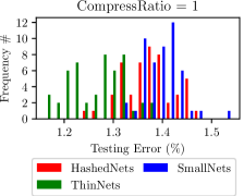
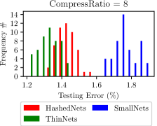
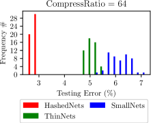
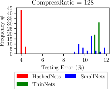
Figure 1: (a) Ratio$=1$; (b) ratio$=8$; (c) ratio$=64$; (d) ratio$=128$. We run two one-hidden layer algorithms on MNIST dataset. Comparison of accuracy distribution with different random seeds for HashedNets and SmallNets. Choose 50 random seeds in total. HashedNets have 1000 hidden units in this case.

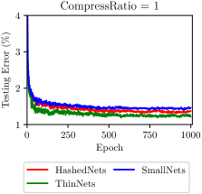
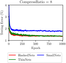
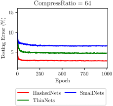
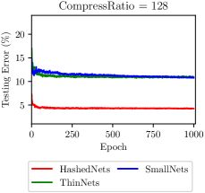
Figure 2: (a) Ratio$=1$; (b) ratio$=8$; (c) ratio$=64$; (d) ratio$=128$. The testing error during training of different networks with random seed 100.

The HashedNets were implemented in Torch7 Collobert et al. (2011); Chen et al. (2015) and validated on NVIDIA GTX 1080 GPU. We used 32 bit precision floating point numbers throughout the experiments. Stochastic gradient descent was adopted as the numerical optimizer with a dropout keep rate of 0.9, momentum of 0.9, and a batch size of 50. ReLU was used as the activation function. We ran 1000 epochs for each experiment and experiments on two single-hidden-layer HashedNets with 500 and 1000 hidden units are conducted, respectively. The amount of units in SmallNets and ThinNets is adjusted to match the amount of weights in HashedNets.

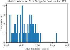
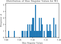
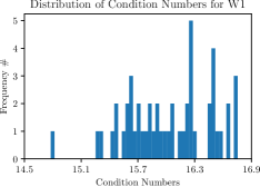
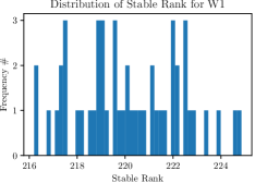
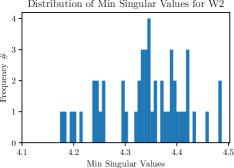
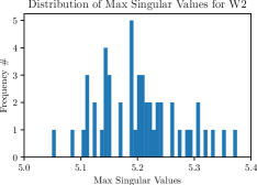
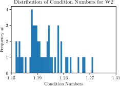
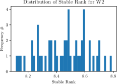
Figure 3: Input dimension is 784. Distributions of singular values, condition numbers, and stable ranks for two weight matrices $W_{1}$ and $W_{2}$ in HashedNets with 1000 hidden units for 50 random seeds.

For different compression ratios, we plot the distribution of testing errors for 50 runs of HashedNets, ThinNets, and SmallNets with 50 different random seeds, as shown in Figure 1. Due to random initialization, SmallNets still gives different results with independent runs. In Figure 1(a), when the compression ratio is 1, which indicating no compression, the distributions for both HashedNets and SmallNets are very close, i.e., with means of 1.37% and 1.40%, standard deviations of 0.050% and 0.038%, respectively. ThinNets provides slightly better testing error with a mean of 1.27% and a standard deviation of 0.057%. In Figure 1(b), when the compression ratio is 8, HashedNets provides smaller testing errors than that of SmallNets, i.e., with means of 1.43% v.s. 1.76%, and standard deviations of 0.052% v.s. 0.070%, respectively. ThinNets provides slightly better testing errors than that of HashedNets, i.e., with means of 1.32% v.s. 1.44%, and standard deviations of 0.060% v.s. 0.056%. In other words, both HashedNets and ThinNets can achieve higher and more robust accuracy with improvements in both mean and standard deviation than SmallNets for this compression ratio. With the compression ratio increasing to 64, as shown in Figure 1(c), the benefit of HashedNets is more significant. The mean of testing errors for HashedNets degrades to 2.80%, while that for SmallNets increases to 6.09%. The errors for SmallNets are more instable due to larger standard deviations. Meanwhile, HashedNets can also provide better accuracy than ThinNets, i.e., with means of 2.80% v.s. 5.03%, and standard deviations of 0.090% v.s. 0.196%. When the compression ratio is 128, as shown in Figure 1(d), HashedNets achieves a mean accuracy of 4.20% and a standard deviation of 0.116%, which is much better than that of ThinNets, a mean accuracy of 11.09% and a standard deviation of 0.160%, and that of SmallNets, a mean accuracy of 10.28% and a standard deviation of 0.810%. In summary, from the aspect of accuracy degradation, when the compression ratio increases from 1 to 128, there is on average 2.83% degradation in accuracy for HashedNets, while the accuracy of SmallNets degrades by 8.88% and that of ThinNets degrades by 9.82%. ThinNets may achieve comparable error to HashedNet for small compression ratios (e.g., 1 and 8), while for large compression ratio, HashedNet tends to be more stable.

Figure 2 plots the training curves of different networks under different compression ratios with random seed 100. The testing errors align with the observation from Figure 1. That is, HashedNets provides high and stable accuracy across various compression ratios; ThinNets achieves good accuracy for small compression ratios (e.g., 1 and 8, the accuracy is close to that of HashedNets), while degrades significantly with the increase of compression ratios; SmallNets are also very sensitive to large compression ratios like ThinNets.

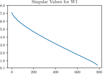
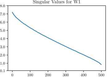
Figure 4: Input dimension is 784. Example of singular values of weight matrix $W_{1}$ in HashedNets with (a) (left) 1000 hidden units and (b) (right) 500 hidden units from large to small for one random seed.

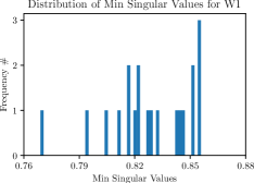
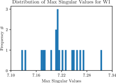
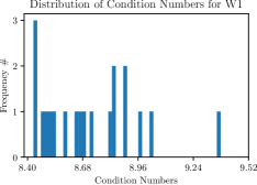
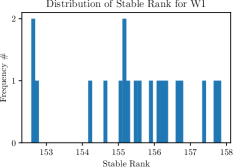
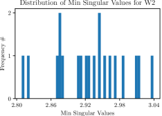
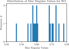
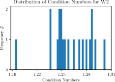
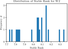
Figure 5: Input dimension is 784. Distributions of singular values, condition numbers, and stable ranks for two weight matrices $W_{1}$ and $W_{2}$ in HashedNets with 500 hidden units for 20 random seeds.

We further verify the full rank assumption of weight matrices in HashedNets. Figure 3 plots the distributions of minimum and maximum singular values, condition numbers, and stable ranks of the two weight matrices $W_{1}$ and $W_{2}$ in HashedNets with 1000 hidden units. The dimensions of $W_{1}$ is $1000\times 784$ and that of $W_{2}$ is $10\times 1000$. The distributions are extracted from the aforementioned 50 runs. Figure 4 (in the Appendix) gives one example of all singular values sorted from large to small in one experiment. All the singular values and condition numbers are distributed in reasonable scales, i.e., neither too close to zero, nor too large. This experiment indicates that the assumption of full rank holds in practice. Same set of figures are also provided for HashedNets with 500 hidden units, as shown in Figure 5 (in the Appendix), where the dimensions of $W_{1}$ is $500\times 784$ and that of $W_{2}$ is $10\times 500$.

6 Conclusion

In this paper, we study the theoretical properties of hashing-based neural networks. We show that (i) parameter-reduced neural nets have uniform approximation power on inputs from any low-dimensional subspace or smooth and well-conditioned manifold; (ii) one-hidden-layer HashedNets have similar recovery guarantee to that of fully connected neural nets. We also empirically explore an alternative compression scheme, ThinNets, which is a very interesting direction for further study, so we plan to explore its property and theoretical insights in the future.

Appendix

Appendix A Notation

For any positive integer $n$, we use $[n]$ to denote the set $\{1,2,\cdots,n\}$. For random variable $X$, let $\mathbb{E}[X]$ denote the expectation of $X$ (if this quantity exists). For any vector $x\in\mathbb{R}^{n}$, we use $\|x\|_{2}$ to denote its $\ell_{2}$ norm.

We provide several definitions related to matrix $A$. Let $\det(A)$ denote the determinant of a square matrix $A$. Let $A^{\top}$ denote the transpose of $A$. Let $A^{\dagger}$ denote the Moore-Penrose pseudoinverse of $A$. Let $A^{-1}$ denote the inverse of a full rank square matrix. Let $\|A\|_{F}$ denote the Frobenius norm of matrix $A$. Let $\|A\|$ denote the spectral norm of matrix $A$. Let $\sigma_{i}(A)$ to denote the $i$-th largest singular value of $A$.

For any function $f$, we define $\widetilde{O}(f)$ to be $f\cdot\log^{O(1)}(f)$. In addition to $O(\cdot)$ notation, for two functions $f,g$, we use the shorthand $f\lesssim g$ (resp. $\gtrsim$) to indicate that $f\leq Cg$ (resp. $\geq$) for an absolute constant $C$. We use $f\eqsim g$ to mean $cf\leq g\leq Cf$ for constants $c,C$.

We state a trivial fact that connects $\ell_{2}$ norm with $\ell_{\infty}$ norm.

Fact A.1.

For any vector $x\in\mathbb{R}^{n}$, we have $\|x\|_{2}\leq\sqrt{n}\|x\|_{\infty}$.

Appendix B Neural Subspace Embedding

B.1 Preliminaries

Definition B.1 (Johnson Lindenstrauss Transform, Johnson and Lindenstrauss [1984]).

A random matrix $S\in\mathbb{R}^{k\times n}$ forms a Johnson-Lindenstrauss transform with parameters $\epsilon,\delta,f$, or JLT($\epsilon,\delta,f$) for short, if with probability at least $1-\delta$, for any $f$-element subset $V\subset\mathbb{R}^{n}$, for all $v,v^{\prime}\in V$ it holds that

$$|\langle Sv,Sv^{\prime}\rangle-\langle v,v^{\prime}\rangle|\leq\epsilon\|v\|_{2}\|v^{\prime}\|_{2}.$$

The well-known Count-Sketch matrix from the data stream literature Charikar et al. [2002], Thorup and Zhang [2012] is a sub-space embedding and JL matrix. The definition is provided as follows.

Definition B.2 (Count-Sketch).

Let $S$ denote a $s\times n$ matrix. We choose a random hash function $h:[n]\rightarrow[s]$, and choose a random hash function $\sigma:[n]\rightarrow\{-1,+1\}$. We set

$$S_{j,i}=\begin{cases}\sigma(i)&\text{\leavevmode\nobreak\ if\leavevmode\nobreak\ }j=h(i),\\ 0&\mathrm{\leavevmode\nobreak\ otherwise.}\end{cases}$$

Count-Sketch matrix gives the following subspace embedding result,

Theorem B.3 (Clarkson and Woodruff [2013], Nelson and Nguyên [2013]).

For any $0<\delta<1$, and for $S$ a Count-Sketch matrix $s=O(d^{2}/(\delta\epsilon^{2}))$ rows, then with probability $1-\delta$, for any fixed $n\times d$ matrix $U$, $S$ is a $(1\pm\epsilon)$ $\ell_{2}$-subspace embedding for $U$. The matrix product $S\cdot U$ can be computed in $O(\operatorname{nnz}(U))$ time. Further, all of this holds if the hash function $h$ defining $S$ is only pairwise independent, and the sign function $\sigma$ defining $S$ is only 4-wise independent.

Definition B.4 (Oblivious Subspace Embedding(OSE), Definition 2.2 in Woodruff [2014]).

Suppose $\Pi$ is a distribution on $s\times n$ matrices $S$, where $s$ is a function of $n,d,\epsilon$ and $\delta$. Suppose that with probability at least $1-\delta$, for any fixed $n\times d$ matrix $U$, a matrix $S$ drawn from distribution $\Pi$ has the property that $S$ is a $(1\pm\epsilon)$ $\ell_{2}$-subspace embedding for $U$. Then we call $\Pi$ an $(\epsilon,\delta)$ oblivious $\ell_{2}$-subspace embedding.

Nelson and Nguyên [2013] provides some other constructions for subspace embedding,

Definition B.5 (Sparse-Embedding).

Let $S$ denote a $s\times n$ matrix. For each $i,j$, $S_{i,j}\in\{0,1/\sqrt{t},-1/\sqrt{t}\}$. For a random draw $S$, let $\delta_{i,j}$ be a indicator random variable for the event $S_{i,j}\neq 0$, and write $S_{i,j}=\delta_{i,j}\sigma_{i,j}/\sqrt{t}$, where the $\sigma_{i,j}$ are random signs. $S$ satisfies the following two properties, for each $j\in[n]$, $\sum_{i=1}^{s}\delta_{i,j}=t$; for any set $T\subseteq[s]\times[n]$, $\operatorname*{{\bf{E}}}[\prod_{(i,j)\in T}\delta_{i,j}\leq(t/m)^{|T|}]$.

Lemma B.6 (Lemma 2.2 in Woodruff [2014]).

Let $A=\{\mathbb{R}^{n}\leavevmode\nobreak\ |\leavevmode\nobreak\ y=Ux,\forall x\in\mathbb{R}^{d},\|y\|_{2}=1\}$, for any $0<\gamma<1$, there exists a $\gamma$-net ${\cal N}$ of $A$ for which $|{\cal N}|\leq(1+4/\gamma)^{d}$.

B.2 Proof of Theorem 3.4

Proof.

Using Theorem 3.2, we choose $s=d\epsilon^{\prime-2}\operatorname{poly}\log(nd/(\epsilon^{\prime}\delta))$, with probability $1-\delta$, we have : for $n_{2}$ fixed vectors $w_{1},\cdots,w_{n_{2}}$ and for all $x\in\text{colspan}(U)$,

$$|\langle Sw_{i},Sx\rangle-\langle w_{i},x\rangle|\leq\epsilon^{\prime}\|w_{i}\|_{2}\|x\|_{2},\forall i\in[n_{1}].$$

Using the Lipschitz property of $\phi_{i}$, we can show that

$$|\phi_{i}(w_{i}^{\top}x)-\phi_{i}(\langle Sw_{i},Sx\rangle)|\leq \leavevmode\nobreak\ L|w_{i}^{\top}x-\langle Sw_{i},Sx\rangle|$$

$$\leq \leavevmode\nobreak\ L\epsilon^{\prime}\|w_{i}\|_{2}\|x\|_{2}$$

$$\leq \leavevmode\nobreak\ \epsilon^{\prime}LBA,$$ (1)

where the first step follows by Property of function $\phi_{i}$, the last step follows by $\|w_{i}\|_{2}\leq B,\|x\|_{2}\leq A$. It remains to bound

$$\left|\sum_{i=1}^{n_{2}}v_{i}\phi_{i}(w_{i}^{\top}x)-v_{i}\phi_{i}(w_{i}^{\top}S^{\top}Sx)\right|\leq \leavevmode\nobreak\ \sum_{i=1}^{n_{2}}|v_{i}|\cdot|\phi_{i}(w_{i}^{\top}x)-\phi_{i}(w_{i}^{\top}S^{\top}Sx)|$$

$$\leq \leavevmode\nobreak\ \|v\|_{1}\max_{i\in[n_{2}]}|\phi_{i}(w_{i}^{\top}x)-\phi_{i}(w_{i}^{\top}S^{\top}Sx)|$$

$$\leq \leavevmode\nobreak\ \|v\|_{1}\epsilon^{\prime}LBA\leq\leavevmode\nobreak\ \epsilon^{\prime}LB^{2}A\leq\leavevmode\nobreak\ \epsilon,$$

where the first step follows by triangle inequality, the third step follows by Eq. (B.2), the fourth step follows by $\|v\|_{1}\leq B$, and the last step follows from $\epsilon^{\prime}=\Theta(\epsilon/(B^{2}AL))$. Therefore, it suffices to choose

$$s=dB^{4}A^{2}L^{2}\epsilon^{-2}\operatorname{poly}\log(nBAL/(\epsilon\delta)).$$

∎

B.3 Proof of Theorem 3.5

Proof.

The proof includes three steps. The first step is similar to the proof of Theorem 3.4. Using Theorem 3.2, we choose $s_{1}=d\epsilon_{1}^{-2}\operatorname{poly}\log(nd/(\epsilon_{1}\delta))$, with probability $1-\delta/2$, we have : for $n_{2}$ fixed vectors $w_{1},\cdots,w_{n_{2}}$ and for all $x\in\text{colspan}(U)$, $|\langle S_{1}w_{i},S_{1}x\rangle-\langle w_{i},x\rangle|\leq\epsilon_{1}\|w_{i}\|_{2}\|x\|_{2},\forall i\in[n_{2}].$ Next, we consider the column space of $U$, which we call $P_{1}$, defined as follows

$$P_{1}=\{y_{1}\in\mathbb{R}^{n_{1}}\leavevmode\nobreak\ |\leavevmode\nobreak\ y_{1}=Ux,\|y_{1}\|_{2}\leq 1,\forall x\in\mathbb{R}^{d}\}.$$

Let ${\cal N}_{1}$ denote the $\gamma_{1}$-net of $P_{1}$, by Lemma B.6, $|{\cal N}_{1}|=2^{O(d\log(1/\gamma_{1}))}$. By definition, for each $y_{1}\in P_{1}$, there exists a vector $z\in{\cal N}_{1}$ such that $\|y_{1}-z_{1}\|_{2}\leq\gamma_{1}.$

Let $P_{2}$ and ${\cal N}_{2}$ be defined as follows,

$$P_{2}= \leavevmode\nobreak\ \{y_{2}\in\mathbb{R}^{n_{2}}\leavevmode\nobreak\ |\leavevmode\nobreak\ y_{2}=\phi(W^{\top}S_{1}^{\top}S_{1}y_{1}),\forall y_{1}\in P_{1}\}.$$

$${\cal N}_{2}= \leavevmode\nobreak\ \{z_{2}\in\mathbb{R}^{n_{2}}\leavevmode\nobreak\ |\leavevmode\nobreak\ z_{2}=\phi(W^{\top}S_{1}^{\top}S_{1}z_{1}),\forall z_{1}\in{\cal N}_{1}\}.$$

Then we want to show the following claim. (The proof can be found in Appendix B.4)

Claim B.7.

(Recursive $\epsilon$-net). Let $\gamma_{2}=\gamma_{1}/(\sqrt{n_{2}}L(1+\epsilon_{1})B)$, then ${\cal N}_{2}$ is an $\gamma_{2}$-net to $P_{2}$.

Now, we choose a sketching matrix $S_{2}\in\mathbb{R}^{s_{2}\times n_{2}}$ with $s_{2}=d\epsilon_{2}^{-2}\operatorname{poly}(nd/(\epsilon_{2}\delta))$, with probability $1-\delta/2$, we have : a vector $v\in\mathbb{R}^{n_{2}}$ and for all $y_{1}\in P_{2}$,

$$|\langle S_{2}v,S_{2}y_{2}\rangle-\langle v,y_{2}\rangle|\leq\epsilon_{2}\|v\|_{2}\|y_{2}\|_{2}.$$

Using triangle inequality, we can bound the error term,

$$|\langle v,\phi(W^{\top}x)\rangle-\langle S_{2}v,S_{2}\phi(W^{\top}S_{1}^{\top}S_{1}x)\rangle|\leq \leavevmode\nobreak\ |\langle v,\phi(W^{\top}x)\rangle-\langle v,\phi(W^{\top}S_{1}^{\top}S_{1}x)\rangle|$$

$$+ \leavevmode\nobreak\ |\langle v,\phi(W^{\top}S_{1}^{\top}S_{1}x)\rangle-\langle S_{2}v,S_{2}\phi(W^{\top}S_{1}^{\top}S_{1}x)\rangle|$$

$$\lesssim \leavevmode\nobreak\ \epsilon_{2}LB^{2}A+\epsilon_{1}B^{2}AL\leq\leavevmode\nobreak\ \epsilon,$$

where the first step follows from triangle inequality, the second step follows from the Property of $S_{2}$, the third step follows from Claim B.8 and Claim B.9, and the last step follows from $\epsilon_{1},\epsilon_{2}\lesssim\epsilon/(LB^{2}A)$. ∎

We list the two Claims here and delay the proofs into Appendix B.4.

Claim B.8.

$|\langle v,\phi(W^{\top}S_{1}^{\top}S_{1}x)\rangle-\langle S_{2}v,S_{2}\phi(W^{\top}S_{1}^{\top}S_{1}x)\rangle|\lesssim\epsilon_{2}LB^{2}A.$

Claim B.9.

$|\langle v,\phi(W^{\top}x)-\langle v,\phi(W^{\top}S_{1}^{\top}S_{1}x)\rangle|\leq LB^{2}A\epsilon_{1}.$

B.4 One hidden layer

In this Section, we provide the proofs of some Claims used for one hidden layer case.

Claim B.7.

Proof.

For each point $y_{2}\in P_{2}$, there must exists a point $y_{1}\in P_{1}$ such that $y_{2}=\phi(W^{\top}S_{1}^{\top}S_{1}y_{1}).$

Since $y_{1}\in P_{1}$ and ${\cal N}_{1}$ is the $\epsilon_{1}$-net of $P_{1}$. Thus, there must exists a vector $z_{1}\in{\cal N}_{1}$ such that $\|y_{1}-z_{1}\|_{2}\leq\gamma_{1}.$

According to the definition ${\cal N}_{2}$, there must exists a point $z_{2}\in{\cal N}_{2}$ such that $z_{2}=\phi(W_{1}^{\top}S_{1}^{\top}S_{1}z_{1}).$ Now, let’s consider the $\|y_{2}-z_{2}\|_{2}$,

$$\|y_{2}-z_{2}\|_{2}\leq \leavevmode\nobreak\ \sqrt{n_{2}}\|y_{2}-z_{2}\|_{\infty}$$

$$= \leavevmode\nobreak\ \sqrt{n_{2}}\|\phi(W^{\top}S_{1}^{\top}S_{1}y_{1})-\phi(W^{\top}S_{1}^{\top}S_{1}z_{1})\|_{\infty}$$

$$= \leavevmode\nobreak\ \sqrt{n_{2}}\max_{i\in[n_{2}]}|\phi_{i}(w_{i}^{\top}S_{1}^{\top}S_{1}y_{1})-\phi_{i}(w_{i}^{\top}S_{1}^{\top}S_{1}z_{1})|$$

$$\leq \leavevmode\nobreak\ \sqrt{n_{2}}\max_{i\in[n_{2}]}L|w_{i}^{\top}S_{1}^{\top}S_{1}y_{1}-w_{i}^{\top}S_{1}^{\top}S_{1}z_{1}|$$

$$= \leavevmode\nobreak\ \sqrt{n_{2}}\max_{i\in[n_{2}]}L|\langle S_{1}w_{i},S_{1}(y_{1}-z_{1})\rangle|$$

$$\leq \leavevmode\nobreak\ \sqrt{n_{2}}\max_{i\in[n_{2}]}L(1+\epsilon_{1})\|w_{i}\|_{2}\|y_{1}-z_{1}\|_{2}$$

$$\leq \leavevmode\nobreak\ \sqrt{n_{2}}L(1+\epsilon_{1})B\gamma_{1}\leq\leavevmode\nobreak\ \gamma_{2},$$

where the first step follows from $\|\cdot\|_{2}\leq\sqrt{\text{dim}}\cdot\|\cdot\|_{\infty}$, the second step follows from definition of $y_{1}$ and $z_{1}$, the third step follows from the definition of $\|\cdot\|_{\infty}$, the fourth step follows from the property of the activation function ($L$-Lipshitz), the sixth step follows from that $S_{1}$ provides a subspace embedding, and the last step follows from the definition of $\gamma_{2}$. ∎

Claim B.8.

$|\langle v,\phi(W^{\top}S_{1}^{\top}S_{1}x)\rangle-\langle S_{2}v,S_{2}\phi(W^{\top}S_{1}^{\top}S_{1}x)\rangle|\lesssim\epsilon_{2}LB^{2}A.$

Proof.

$$|\langle v,\phi(W^{\top}S_{1}^{\top}S_{1}x)\rangle-\langle S_{2}v,S_{2}\phi(W^{\top}S_{1}^{\top}S_{1}x)\rangle|\leq \leavevmode\nobreak\ \epsilon_{2}\|v\|_{2}\cdot\|\phi(W^{\top}S_{1}^{\top}S_{1}x)\|_{2}$$

$$\leq \leavevmode\nobreak\ \epsilon_{2}\|v\|_{2}\cdot L\max_{i\in[n_{2}]}|w_{i}^{\top}S_{1}^{\top}S_{1}x|$$

$$\leq \leavevmode\nobreak\ \epsilon_{2}\|v\|_{2}\cdot L\max_{i\in[n_{2}]}(1\pm\epsilon_{1})\|w_{i}\|_{2}\|x\|_{2}$$

$$\lesssim \leavevmode\nobreak\ \epsilon_{2}LB^{2}A,$$

where the first step follows from that $S_{2}$ is a $(1\pm\epsilon_{2})$ $\ell_{2}$ subspace embedding, the second step follows from the property of $\phi_{i}$ ($L$-lipshitz), the third step follows from that $S_{1}$ is $(1\pm\epsilon_{1})$ $\ell_{2}$ subspace embedding, the fourth step follows from that $\|v\|_{2},\|W\|_{2}\leq B$ and $\|x\|_{2}\leq A$. ∎

Claim B.9.

$|\langle v,\phi(W^{\top}x)-\langle v,\phi(W^{\top}S_{1}^{\top}S_{1}x)\rangle|\leq LB^{2}A\epsilon_{1}.$

Proof.

$$|\langle v,\phi(W^{\top}x)-\langle v,\phi(W^{\top}S_{1}^{\top}S_{1}x)\rangle|\leq \leavevmode\nobreak\ \|v\|_{2}\cdot\|\phi(W^{\top}x)-\phi(W^{\top}S_{1}^{\top}S_{1}x)\|_{2}$$

$$\leq \leavevmode\nobreak\ \|v\|_{2}\cdot L\max_{i\in[n_{2}]}|w_{i}^{\top}x-w_{i}^{\top}S_{1}^{\top}S_{1}x|$$

$$\leq \leavevmode\nobreak\ \|v\|_{2}L\epsilon_{1}\max_{i\in[n_{2}]}\|w_{i}\|_{2}\|x\|_{2}$$

$$\leq \leavevmode\nobreak\ LB^{2}A\epsilon_{1},$$

where the first step follows from Cauchy-Shawrz inequality, the second step follow by property of activation function, the third step follows from $S_{1}$ is an $(1\pm\epsilon_{1})$ subspace embedding, and last step follows from that $\|v\|_{2},\|W\|_{2}\leq B$, $\|x\|_{2}\leq A$. ∎

B.5 Two hidden layers

The goal of section is to present Theorem B.10.

Theorem B.10 (Neural oblivious subspace embedding two hidden layer neural networks).

Given parameters $n_{3}\geq 1,n_{2}\geq 1,n_{2}\geq 1,\epsilon\in(0,1),\delta\in(0,1)$ and $n=\max(n_{3},n_{2},n_{1})$. Given $n_{2}$ activation functions $\phi_{1,i}:\mathbb{R}\rightarrow\mathbb{R}$ with $L$-Lipshitz and normalized by $1/\sqrt{n_{2}}$, $n_{3}$ activation functions $\phi_{2,i}:\mathbb{R}\rightarrow\mathbb{R}$ with $L$-Lipshitz and normalized by $1/\sqrt{n_{3}}$, a fixed matrix $U\in\mathbb{R}^{n_{1}\times d}$, two weight matrices $W_{1}\in\mathbb{R}^{n_{2}\times n_{1}}$ and $W_{2}\in\mathbb{R}^{n_{3}\times n_{2}}$ with (the $i_{1}$-th column of $W_{1}$) $w_{1,i_{1}}\in{\cal B}_{2}(B,n_{1})$ and (the $i_{2}$-th column of $W_{2}$) $w_{2,i_{2}}\in{\cal B}_{2}(B,n_{2})$, a weight vector $v\in\mathbb{R}^{n_{3}}$ with $v\in{\cal B}_{2}(B,n_{3})$. Choose a SparseEmbedding matrix $S_{1}\in\mathbb{R}^{s_{1}\times n_{1}}$, $S_{2}\in\mathbb{R}^{s_{2}\times n_{2}}$, $S_{3}\in\mathbb{R}^{s_{3}\times n_{3}}$ with

$$s_{1},s_{2},s_{3}=O(dL^{4}B^{6}A^{2}\epsilon^{-2}\operatorname{poly}\log(nLBA/(\epsilon\delta))),$$

then with probability $1-\delta$, we have : for all $x\in\mathrm{colspan}(U)\cap{\cal B}_{2}(A,n_{1})$,

$$|\langle v,\phi_{2}(W_{2}^{\top}\phi_{1}(W_{1}^{\top}x))\rangle-\langle S_{3}v,S_{3}\phi_{2}(W_{2}^{\top}S_{2}^{\top}S_{2}\phi_{1}(W_{1}^{\top}S_{1}^{\top}S_{1}x))\rangle|\leq\epsilon.$$

Proof.

It follows by combining Section B.5.1 and Lemma B.13. ∎

B.5.1 Recursive $\epsilon$-net argument

Using Theorem 3.2, we choose $s_{1}=d\epsilon_{1}^{-2}\operatorname{poly}\log(nd/(\epsilon_{1}\delta))$, with probability $1-\delta/2$, we have : for $n_{2}$ fixed vectors $w_{1},\cdots,w_{n_{2}}$ and for all $x\in\text{colspan}(U)$,

$$|\langle S_{1}w_{i},S_{1}x\rangle-\langle w_{i},x\rangle|\leq\epsilon_{1}\|w_{i}\|_{2}\|x\|_{2},\forall i\in[n_{2}].$$

We define $P_{1}$ as follows

$$P_{1}=\{y_{1}\in\mathbb{R}^{n_{1}}\leavevmode\nobreak\ |\leavevmode\nobreak\ y_{1}=Ux,\|y_{1}\|_{2}\leq 1,\forall x\in\mathbb{R}^{d}\}.$$

Let ${\cal N}_{1}$ denote the $\gamma_{1}$-net of $P_{1}$, by Lemma B.6, $|{\cal N}_{1}|=2^{O(d\log(1/\gamma_{1}))}$. By definition For each $y_{1}\notin P_{1}$, there exists a vector $z\in{\cal N}_{1}$ such that

$$\|y_{1}-z_{1}\|_{2}\leq\gamma_{1}.$$

Let $P_{2}$ be defined as follows,

$$P_{2}=\{y_{2}\in\mathbb{R}^{n_{2}}\leavevmode\nobreak\ |\leavevmode\nobreak\ y_{2}=\phi_{1}(W_{1}^{\top}S_{1}^{\top}S_{1}y_{1}),\forall y_{1}\in P_{1}\}.$$

We define ${\cal N}_{2}$ to be

$${\cal N}_{2}=\{z_{2}\in\mathbb{R}^{n_{2}}\leavevmode\nobreak\ |\leavevmode\nobreak\ z_{2}=\phi_{1}(W_{1}^{\top}S_{1}^{\top}S_{1}z_{1}),\forall z_{1}\in{\cal N}_{1}\}.$$

Then we want to show

Claim B.11.

Let $\gamma_{2}=\gamma_{1}/(L(1+\epsilon_{1})B)$, then ${\cal N}_{2}$ is an $\gamma_{2}$-net to $P_{2}$.

Proof.

For each point $y_{2}\in P_{2}$, there must exists a point $y_{1}\in P_{1}$ such that

$$y_{2}=\phi(W_{1}^{\top}S_{1}^{\top}S_{1}y_{1}).$$

Since $y_{1}\in P_{1}$ and ${\cal N}_{1}$ is the $\epsilon_{1}$-net of $P_{1}$. Thus, there must exists a vector $z_{1}\in{\cal N}_{1}$ such that

$$\|y_{1}-z_{1}\|_{2}\leq\gamma_{1}.$$

According to the definition ${\cal N}_{2}$, there must exists a point $z_{2}\in{\cal N}_{2}$ such that

$$z_{2}=\phi(W_{1}^{\top}S_{1}^{\top}S_{1}z_{1}).$$

Now, let’s consider the $\|y_{2}-z_{2}\|_{2}$,

$$\|y_{2}-z_{2}\|_{2}\leq \leavevmode\nobreak\ \sqrt{n_{2}}\|y_{2}-z_{2}\|_{\infty}$$

$$= \leavevmode\nobreak\ \sqrt{n_{2}}\|\phi_{1}(W_{1}^{\top}S_{1}^{\top}S_{1}y_{1})-\phi_{1}(W_{1}^{\top}S_{1}^{\top}S_{1}z_{1})\|_{\infty}$$

$$= \leavevmode\nobreak\ \sqrt{n_{2}}\max_{i\in[n_{2}]}|\phi_{1}(w_{1,i_{1}}^{\top}S_{1}^{\top}S_{1}y_{1})-\phi_{1}(w_{1,i_{1}}^{\top}S_{1}^{\top}S_{1}z_{1})|$$

$$= \leavevmode\nobreak\ \max_{i_{1}\in[n_{2}]}L|w_{1,i_{1}}^{\top}S_{1}^{\top}S_{1}y_{1}-w_{1,i_{1}}^{\top}S_{1}^{\top}S_{1}z_{1}|$$

$$= \leavevmode\nobreak\ \max_{i_{1}\in[n_{2}]}L|\langle S_{1}w_{1,i_{1}},S_{1}(y_{1}-z_{1})\rangle|$$

$$\leq \leavevmode\nobreak\ \max_{i_{1}\in[n_{2}]}L(1+\epsilon_{1})\|w_{1,i_{1}}\|_{2}\|y_{1}-z_{1}\|_{2}$$

$$\leq \leavevmode\nobreak\ L(1+\epsilon_{1})B\gamma_{1}$$

$$\leq \leavevmode\nobreak\ \gamma_{2},$$

where the first step follows by $\|\cdot\|_{2}\leq\sqrt{\text{dim}}\cdot\|\cdot\|_{\infty}$, the second step follows by definition of $y_{1}$ and $z_{1}$, the third step follows by definition, the fourth step follows by property of activation function ($L$-lipshitz and normalization), the sixth step follows by $S_{1}$ provides a subspace embedding, the last step follows by definition of $\gamma_{2}$. ∎

It is obvious that $|{\cal N}_{2}|=|{\cal N}_{1}|$.

Let $P_{3}$ be defined as follows,

$$P_{3}=\{y_{3}\in\mathbb{R}^{n_{3}}\leavevmode\nobreak\ |\leavevmode\nobreak\ y_{3}=\phi_{2}(W_{2}^{\top}S_{2}^{\top}S_{2}y_{2}),\forall y_{2}\in P_{2}\}.$$

We define ${\cal N}_{2}$ to be

$${\cal N}_{3}=\{z_{3}\in\mathbb{R}^{n_{3}}\leavevmode\nobreak\ |\leavevmode\nobreak\ z_{3}=\phi_{2}(W_{2}^{\top}S_{2}^{\top}S_{2}z_{2}),\forall z_{2}\in{\cal N}_{2}\}.$$

Then we want to show

Claim B.12.

Let $\gamma_{3}=\gamma_{2}/(L(1+\epsilon_{2})B)$, then ${\cal N}_{3}$ is an $\gamma_{3}$-net to $P_{3}$.

Proof.

For each point $y_{3}\in P_{3}$, there must exists a point $y_{2}\in P_{2}$ such that

$$y_{3}=\phi(W_{2}^{\top}S_{2}^{\top}S_{2}y_{2}).$$

Since $y_{2}\in P_{2}$ and ${\cal N}_{2}$ is the $\epsilon_{2}$-net of $P_{2}$. Thus, there must exists a vector $z_{2}\in{\cal N}_{2}$ such that

$$\|y_{2}-z_{2}\|_{2}\leq\gamma_{2}.$$

According to the definition ${\cal N}_{3}$, there must exists a point $z_{3}\in{\cal N}_{3}$ such that

$$z_{3}=\phi(W_{2}^{\top}S_{2}^{\top}S_{2}z_{2}).$$

Now, let’s consider the $\|y_{3}-z_{3}\|_{2}$,

$$\|y_{3}-z_{3}\|_{2}\leq \leavevmode\nobreak\ \sqrt{n_{3}}\|y_{3}-z_{3}\|_{\infty}$$

$$= \leavevmode\nobreak\ \sqrt{n_{3}}\|\phi_{2}(W_{2}^{\top}S_{2}^{\top}S_{2}y_{2})-\phi_{2}(W_{2}^{\top}S_{2}^{\top}S_{2}z_{2})\|_{\infty}$$

$$= \leavevmode\nobreak\ \sqrt{n_{3}}\max_{i\in[n_{3}]}|\phi_{2}(w_{2,i_{2}}^{\top}S_{2}^{\top}S_{2}y_{2})-\phi_{1}(w_{2,i_{2}}^{\top}S_{2}^{\top}S_{2}z_{2})|$$

$$= \leavevmode\nobreak\ \max_{i_{2}\in[n_{3}]}L|w_{2,i_{2}}^{\top}S_{2}^{\top}S_{2}y_{2}-w_{2,i_{2}}^{\top}S_{2}^{\top}S_{2}z_{2}|$$

$$= \leavevmode\nobreak\ \max_{i_{2}\in[n_{3}]}L|\langle S_{2}w_{2,i_{2}},S_{2}(y_{2}-z_{2})\rangle|$$

$$\leq \leavevmode\nobreak\ \max_{i_{2}\in[n_{3}]}L(1+\epsilon_{2})\|w_{2,i_{2}}\|_{2}\|y_{2}-z_{2}\|_{2}$$

$$\leq \leavevmode\nobreak\ L(1+\epsilon_{2})B\gamma_{2}$$

$$\leq \leavevmode\nobreak\ \gamma_{3},$$

where the first step follows by $\|\cdot\|_{2}\leq\sqrt{\text{dim}}\cdot\|\cdot\|_{\infty}$, the second step follows by definition of $y_{2}$ and $z_{2}$, the third step follows by definition, the fourth step follows by property of activation function ($L$-lipshitz and normalization), the sixth step follows by $S_{2}$ provides a subspace embedding, the last step follows by definition of $\gamma_{3}$. ∎

B.5.2 Bounding the error

Lemma B.13 (Bounding the error).

$$|\langle v,\phi_{2}(W_{2}^{\top}\phi_{1}(W_{1}^{\top}x))\rangle-\langle S_{3}v,S_{3}\phi_{2}(W_{2}^{\top}S_{2}^{\top}S_{2}\phi_{1}(W_{1}^{\top}S_{1}^{\top}S_{1}x))\rangle|\leq 2(\epsilon_{1}+\epsilon_{2}+\epsilon_{3})L^{2}B^{3}A.$$

Proof.

$$\leavevmode\nobreak\ |\langle v,\phi_{2}(W_{2}^{\top}\phi_{1}(W_{1}^{\top}x))\rangle-\langle S_{3}v,S_{3}\phi_{2}(W_{2}^{\top}S_{2}^{\top}S_{2}\phi_{1}(W^{\top}S_{1}^{\top}S_{1}x))\rangle|$$

$$\leq \leavevmode\nobreak\ |\langle v,\phi_{2}(W_{2}^{\top}\phi_{1}(W_{1}^{\top}x))\rangle-\langle v,\phi_{2}(W_{2}^{\top}\phi_{1}(W_{1}^{\top}S_{1}^{\top}S_{1}x))\rangle|$$

$$+ \leavevmode\nobreak\ |\langle v,\phi_{2}(W_{2}^{\top}\phi_{1}(W_{1}^{\top}S_{1}^{\top}S_{1}x))\rangle-\langle v,\phi_{2}(W_{2}^{\top}S_{2}^{\top}S_{2}\phi_{1}(W_{1}^{\top}S_{1}^{\top}S_{1}x))\rangle|$$

$$+ \leavevmode\nobreak\ |\langle v,\phi_{2}(W_{2}^{\top}S_{2}^{\top}S_{2}\phi_{1}(W_{1}^{\top}S_{1}^{\top}S_{1}x))-\langle S_{3}v,S_{3}\phi_{2}(W_{2}^{\top}S_{2}^{\top}S_{2}\phi_{1}(W_{1}^{\top}S_{1}^{\top}S_{1}x))\rangle|$$

$$\leq \leavevmode\nobreak\ 2(\epsilon_{1}+\epsilon_{2}+\epsilon_{3})L^{2}B^{3}A,$$

where the first step follows by triangle inequality, and the last step follows by Claim B.14, B.15, B.16. ∎

Claim B.14.

$|\langle v,\phi_{2}(W_{2}^{\top}\phi_{1}(W_{1}^{\top}x))\rangle-\langle v,\phi_{2}(W_{2}^{\top}\phi_{1}(W_{1}^{\top}S_{1}^{\top}S_{1}x))\rangle|\leq\epsilon_{1}L^{2}B^{3}A$.

Proof.

We have,

$$\leavevmode\nobreak\ |\langle v,\phi_{2}(W_{2}^{\top}\phi_{1}(W_{1}^{\top}x))\rangle-\langle v,\phi_{2}(W_{2}^{\top}\phi_{1}(W_{1}^{\top}S_{1}^{\top}S_{1}x))\rangle|$$

$$\leq \leavevmode\nobreak\ \|v\|_{2}\cdot\|\phi_{2}(W_{2}^{\top}\phi_{1}(W_{1}^{\top}x))-\phi_{2}(W_{2}^{\top}\phi_{1}(W_{1}^{\top}S_{1}^{\top}S_{1}x))\|_{2}$$

$$\leq \leavevmode\nobreak\ \|v\|_{2}\cdot\sqrt{n_{3}}\cdot\max_{i_{2}\in[n_{3}]}|\phi_{2}(w_{2,i_{2}}^{\top}\phi_{1}(W_{1}^{\top}x))-\phi_{2}(w_{2,i_{2}}^{\top}\phi_{1}(W_{1}^{\top}S_{1}^{\top}S_{1}x))|$$

$$\leq \leavevmode\nobreak\ \|v\|_{2}\cdot L\cdot\max_{i_{2}\in[n_{3}]}|w_{2,i_{2}}^{\top}\phi_{1}(W_{1}^{\top}x)-w_{2,i_{2}}^{\top}\phi_{1}(W_{1}^{\top}S_{1}^{\top}S_{1}x)|$$

$$\leq \leavevmode\nobreak\ \|v\|_{2}\cdot L\cdot\max_{i_{2}\in[n_{3}]}\|w_{2,i_{2}}\|_{2}\|\phi_{1}(W_{1}^{\top}x)-\phi_{1}(W_{1}^{\top}S_{1}^{\top}S_{1}x)\|_{2}$$

$$\leq \leavevmode\nobreak\ \|v\|_{2}\cdot L\cdot\max_{i_{2}\in[n_{3}]}\|w_{2,i_{2}}\|_{2}\max_{i_{1}\in[n_{2}]}\sqrt{n_{2}}L|\phi_{1}(w_{1,i_{1}}^{\top}x)-\phi_{1}(w_{1,i_{1}}^{\top}S_{1}^{\top}S_{1}x)|$$

$$\leq \leavevmode\nobreak\ \|v\|_{2}\cdot L\cdot\max_{i_{2}\in[n_{3}]}\|w_{2,i_{2}}\|_{2}\max_{i_{1}\in[n_{2}]}L|w_{1,i_{1}}^{\top}x-w_{1,i_{1}}^{\top}S_{1}^{\top}S_{1}x|$$

$$\leq \leavevmode\nobreak\ \|v\|_{2}\cdot L\cdot\max_{i_{2}\in[n_{3}]}\|w_{2,i_{2}}\|_{2}\max_{i_{1}\in[n_{2}]}L\epsilon_{1}\|w_{1,i_{1}}\|_{2}\|x\|_{2}$$

$$\leq \leavevmode\nobreak\ \epsilon_{1}L^{2}B^{3}A,$$

where the first step follows by Cauchy-Shawrz inequality, the second step follows by Fact A.1, the third step follows by property of activation function ($L$-Lipshitz and normalization), the fourth step follows by Cauchy-Shawrz inequality, the fifth step follows by Fact A.1, the sixth step follows by property of activation function, the seventh step follows by $S_{1}$ is a $(1\pm\epsilon_{1})$ $\ell_{2}$ subspace embedding, and the last step follows by $\|v\|_{2},\|w_{2,i_{2}}\|_{2},\|w_{1,i_{1}}\|_{2}\leq B$, $\|x\|_{2}\leq A$. ∎

Claim B.15.

$|\langle v,\phi_{2}(W_{2}^{\top}\phi_{1}(W_{1}^{\top}S_{1}^{\top}S_{1}x))\rangle-\langle v,\phi_{2}(W_{2}^{\top}S_{2}^{\top}S_{2}\phi_{1}(W_{1}^{\top}S_{1}^{\top}S_{1}x))\rangle|\leq 2\epsilon_{2}L^{2}B^{3}A$.

Proof.

We have,

$$\leavevmode\nobreak\ |\langle v,\phi_{2}(W_{2}^{\top}\phi_{1}(W_{1}^{\top}S_{1}^{\top}S_{1}x))\rangle-\langle v,\phi_{2}(W_{2}^{\top}S_{2}^{\top}S_{2}\phi_{1}(W_{1}^{\top}S_{1}^{\top}S_{1}x))\rangle|$$

$$\leq \leavevmode\nobreak\ \|v\|_{2}\|\phi_{2}(W_{2}^{\top}\phi_{1}(W_{1}^{\top}S_{1}^{\top}S_{1}x))-\phi_{2}(W_{2}^{\top}S_{2}^{\top}S_{2}\phi_{1}(W_{1}^{\top}S_{1}^{\top}S_{1}x))\|_{2}$$

$$\leq \leavevmode\nobreak\ \|v\|_{2}\cdot\max_{i_{2}\in[n_{3}]}\sqrt{n_{3}}\cdot|\phi_{2}(w_{2,i_{2}}^{\top}\phi_{1}(W_{1}^{\top}S_{1}^{\top}S_{1}x))-\phi_{2}(w_{2,i_{2}}^{\top}S_{2}^{\top}S_{2}\phi_{1}(W_{1}^{\top}S_{1}^{\top}S_{1}x))|$$

$$\leq \leavevmode\nobreak\ \|v\|_{2}\cdot\max_{i_{2}\in[n_{3}]}L\cdot|w_{2,i_{2}}^{\top}\phi_{1}(W_{1}^{\top}S_{1}^{\top}S_{1}x)-w_{2,i_{2}}^{\top}S_{2}^{\top}S_{2}\phi_{1}(W_{1}^{\top}S_{1}^{\top}S_{1}x)|$$

$$\leq \leavevmode\nobreak\ \|v\|_{2}\cdot\max_{i_{2}\in[n_{3}]}L\cdot\epsilon_{2}\cdot\|w_{2,i_{2}}\|_{2}\|\phi_{1}(W_{1}^{\top}S_{1}^{\top}S_{1}x)\|_{2}$$

$$\leq \leavevmode\nobreak\ \|v\|_{2}\cdot\max_{i_{2}\in[n_{3}]}L\cdot\epsilon_{2}\cdot\|w_{2,i_{2}}\|_{2}\max_{i_{1}\in[n_{2}]}\sqrt{n_{2}}|\phi_{1}(w_{1,i_{1}}^{\top}S_{1}^{\top}S_{1}x)|$$

$$\leq \leavevmode\nobreak\ \|v\|_{2}\cdot\max_{i_{2}\in[n_{3}]}L\cdot\epsilon_{2}\cdot\|w_{2,i_{2}}\|_{2}\max_{i_{1}\in[n_{2}]}L|w_{1,i_{1}}^{\top}S_{1}^{\top}S_{1}x|$$

$$\leq \leavevmode\nobreak\ \|v\|_{2}\cdot\max_{i_{2}\in[n_{3}]}L\cdot\epsilon_{2}\cdot\|w_{2,i_{2}}\|_{2}\max_{i_{1}\in[n_{2}]}(1+\epsilon_{1})L\|w_{1,i_{1}}\|_{2}\|x\|_{2}$$

$$\leq \leavevmode\nobreak\ 2\epsilon_{2}L^{2}B^{3}A,$$

where the first step follows by Cauchy-Shawrz inequality, the second step follows by Fact A.1, the third step follows by property of activation function, the fourth step follows by $S_{2}$ is a $(1\pm\epsilon_{2})$ $\ell_{2}$ subspace embedding, the fifth step follows by Fact A.1, the sixth step follows by property of activation function, the seventh step follows by $S_{1}$ is $a$ $(1\pm\epsilon_{1})$ $\ell_{2}$ subspace embedding, and the last step follows by $\|v\|_{2},\|w_{2,i_{2}}\|_{2},\|w_{1,i_{1}}\|_{2}\leq B$ and $\|x\|_{2}\leq A$. ∎

Claim B.16.

$|\langle v,\phi_{2}(W_{2}^{\top}S_{2}^{\top}S_{2}\phi_{1}(W_{1}^{\top}S_{1}^{\top}S_{1}x))-\langle S_{3}v,S_{3}\phi_{2}(W_{2}^{\top}S_{2}^{\top}S_{2}\phi_{1}(W^{\top}S_{1}^{\top}S_{1}x))\rangle|\leq 2\epsilon_{3}L^{2}B^{3}A$.

Proof.

We have

$$\leavevmode\nobreak\ |\langle v,\phi_{2}(W_{2}^{\top}S_{2}^{\top}S_{2}\phi_{1}(W_{1}^{\top}S_{1}^{\top}S_{1}x))-\langle S_{3}v,S_{3}\phi_{2}(W_{2}^{\top}S_{2}^{\top}S_{2}\phi_{1}(W^{\top}S_{1}^{\top}S_{1}x))\rangle|$$

$$\leq \leavevmode\nobreak\ \epsilon_{3}\|v\|_{2}\cdot\|\phi_{2}(W_{2}^{\top}S_{2}^{\top}S_{2}\phi_{1}(W_{1}^{\top}S_{1}^{\top}S_{1}x))\|_{2}$$

$$\leq \leavevmode\nobreak\ \epsilon_{3}\|v\|_{2}\cdot L\max_{i_{2}\in[n_{3}]}|w_{2,i_{2}}^{\top}S_{2}^{\top}S_{2}\phi_{1}(W_{1}^{\top}S_{1}^{\top}S_{1}x)|$$

$$\leq \leavevmode\nobreak\ \epsilon_{3}\|v\|_{2}\cdot L\max_{i_{2}\in[n_{3}]}(1+\epsilon_{2})\|w_{2,i_{2}}\|_{2}\cdot\|\phi_{1}(W_{1}^{\top}S_{1}^{\top}S_{1}x)\|_{2}$$

$$\leq \leavevmode\nobreak\ \epsilon_{3}\|v\|_{2}\cdot L\max_{i_{2}\in[n_{3}]}(1+\epsilon_{2})\|w_{2,i_{2}}\|_{2}\cdot L\max_{i_{1}\in[n_{2}]}|w_{1,i_{1}}^{\top}S_{1}^{\top}S_{1}x|$$

$$\leq \leavevmode\nobreak\ \epsilon_{3}\|v\|_{2}\cdot L\max_{i_{2}\in[n_{3}]}(1+\epsilon_{2})\|w_{2,i_{2}}\|_{2}\cdot L\max_{i_{1}\in[n_{2}]}(1+\epsilon_{1})\|w_{1,i_{1}}\|_{2}\|x\|_{2}$$

$$\leq \leavevmode\nobreak\ 2\epsilon_{3}L^{2}B^{3}A,$$

where the first step follows by $S_{3}$ is a $(1\pm\epsilon_{3})$ $\ell_{2}$ subspace embedding, the second step follows by Fact A.1 and the property of activation function, the third step follows by $S_{2}$ is a $(1\pm\epsilon_{2})$ $\ell_{2}$ subspace embedding, the fourth step follows by Fact A.1, the fifth step follows by $S_{1}$ is a $(1\pm\epsilon_{1})$ $\ell_{1}$ subspace embedding, and last step follows $\|v\|_{2},\|w_{2,i_{2}}\|_{2},\|w_{1,i_{1}}\|_{2}\leq B$ and $\|x\|_{2}\leq A$. ∎

B.6 Multiple hidden layers

The goal of section is to present Theorem B.17.

Theorem B.17 (Oblivious neural subspace embedding multiple hidden layer neural networks, restate of Theorem 3.6).

Given parameters $q\geq 1$, $n_{j}\geq 1,\forall j\in[q+1],\epsilon\in(0,1),\delta\in(0,1)$ and $n=\max_{j\in[q+1]}n_{j}$. For each $j\in[q]$, for each $i\in[n_{j+1}]$ let $\phi_{j,i}:\mathbb{R}\rightarrow\mathbb{R}$ denote an activation function with $L$-Lipshitz and normalized by $1/\sqrt{n_{j+1}}$. Given a fixed matrix $U\in\mathbb{R}^{n_{1}\times d}$, $q$ weight matrices $W_{j}\in\mathbb{R}^{n_{j+1}\times n_{j}},\forall j\in[q]$ with (the $i_{j}$-th column of $W_{j}$) $w_{j,i_{j}}\in{\cal B}_{2}(B,n_{j})$, a weight vector $v\in\mathbb{R}^{n_{j+1}}$ with $v\in{\cal B}_{2}(B,n_{j+1})$. For each $j\in[q+1]$, we choose a SparseEmbedding matrix $S_{1}\in\mathbb{R}^{s_{j}\times n_{j}}$ with

$$s_{j}=O(dq^{2}L^{2q}B^{2q+2}A^{2}\epsilon^{-2}\operatorname{poly}\log(nqLBA/(\epsilon\delta))).$$

Then with probability $1-\delta$, we have : for all $x\in\mathrm{colspan}(U)\cap{\cal B}_{2}(A,n_{1})$,

$$|\langle v,\phi_{q}(W_{q}^{\top}\cdots\phi_{2}(W_{2}^{\top}\phi_{1}(W_{1}^{\top}x)))\rangle-\langle S_{q+1}v,S_{q+1}\phi_{q}(W_{q}^{\top}S_{q}^{\top}S_{q}\cdots\phi_{2}(W_{2}^{\top}S_{2}^{\top}S_{2}\phi_{1}(W_{1}^{\top}S_{1}^{\top}S_{1}x)))\rangle|\leq\epsilon.$$

To provide a clear proof, we define some notations to simplify the multiple hidden layer neural network,

Definition B.18.

We first define the base

$$f^{(0)}(x)=\widetilde{f}^{(0)}(x)=x.$$

Then we define the general case in a recursive way,

$$f^{(j)}(x)= \leavevmode\nobreak\ \phi_{j}(W_{j}^{\top}f^{(j-1)}(x)),\forall j\in[q]$$

$$\widetilde{f}^{(j)}(x)= \leavevmode\nobreak\ \phi_{j}(W_{j}^{\top}S_{j}^{\top}S_{j}\widetilde{f}^{(j-1)}(x)),\forall j\in[q]$$

$$f^{(j,l)}\circ\widetilde{f}^{(l-1)}(x)= \leavevmode\nobreak\ \phi_{j}(W_{j}^{\top}\cdots\phi_{l}(W_{l}^{\top}\widetilde{f}^{(l-1)}(x))),\forall j\in[q],l\in\{1,\cdots,j+1\}.$$

Note that $f^{(j,1)}\circ\widetilde{f}^{(0)}(x)=f^{(j)}(x)$ and $f^{(j,j+1)}\circ\widetilde{f}^{(j)}(x)=\widetilde{f}^{(j)}(x)$.

Using the above definition, it is easy to see that

$$\langle v,\phi_{q}(W_{q}^{\top}\cdots\phi_{2}(W_{2}^{\top}\phi_{1}(W_{1}^{\top}x)))\rangle=\langle v,f^{(q)}(x)\rangle,$$

and

$$\langle S_{q+1}v,S_{q+1}\phi_{q}(W_{q}^{\top}S_{q}^{\top}S_{q}\cdots\phi_{2}(W_{2}^{\top}S_{2}^{\top}S_{2}\phi_{1}(W_{1}^{\top}S_{1}^{\top}S_{1}x)))\rangle=\langle S_{q+1}v,S_{q+1}\widetilde{f}^{(q)}(x)\rangle.$$

Thus, we have

$$\leavevmode\nobreak\ |\langle v,f^{(q)}(x)\rangle-\langle S_{q+1}v,S_{q+1}\widetilde{f}^{(q)}(x)\rangle|$$

$$\leq \leavevmode\nobreak\ \sum_{l=1}^{q}|\langle v,f^{(q,l)}\circ\widetilde{f}^{(l-1)}(x)\rangle-\langle v,f^{(q,l+1)}\circ\widetilde{f}^{(l)}(x)\rangle|+|\langle v,\widetilde{f}^{(q)}(x)-\langle S_{q+1}v,S_{q+1}\widetilde{f}^{(q)}(x)|.$$

Now the question is how to bound the above $q+1$ terms.

Claim B.19.

$|\langle v,\widetilde{f}^{(q)}(x)-\langle S_{q+1}v,S_{q+1}\widetilde{f}^{(q)}(x)|\leq 4\epsilon_{q}L^{q}B^{q+1}A^{q}$.

Proof.

We have,

$$|\langle v,\widetilde{f}^{(q)}(x)-\langle S_{q+1}v,S_{q+1}\widetilde{f}^{(q)}(x)|\leq \leavevmode\nobreak\ \epsilon_{q+1}\|v\|_{2}\cdot\|\widetilde{f}^{(q)}(x)\|_{2}$$

$$\leq \leavevmode\nobreak\ \epsilon_{q+1}L^{q}B^{q+1}A^{q}\prod_{j=1}^{q}(1+\epsilon_{j})$$

$$\leq \leavevmode\nobreak\ 4\epsilon_{q+1}L^{q}B^{q+1}A^{q},$$

where the first step follows by $S_{q+1}$ is a $(1\pm\epsilon_{q+1})$ $\ell_{2}$ subspace embedding, the second step follows by applying the argument in the proof of Lemma B.13 recursively, and the last step follows by $\epsilon_{j}<1/q$. ∎

Similarly, we have

Claim B.20.

$\forall l\in[q],|\langle v,f^{(q,l)}\circ\widetilde{f}^{(l-1)}(x)\rangle-\langle v,f^{(q,l+1)}\circ\widetilde{f}^{(l)}(x)\rangle|\leq 4\epsilon_{l}L^{q}B^{q+1}A^{q}$.

Proof.

We have

$$|\langle v,f^{(q,l)}\circ\widetilde{f}^{(l-1)}(x)\rangle-\langle v,f^{(q,l+1)}\circ\widetilde{f}^{(l)}(x)\rangle|\leq \leavevmode\nobreak\ \epsilon_{l}L^{q}B^{q+1}A^{q}\prod_{i=l-1}^{1}(1+\epsilon_{i})$$

$$\leq \leavevmode\nobreak\ 4\epsilon_{l}L^{q}B^{q+1}A^{q},$$

where the first step follows by applying the argument in the proof of Lemma B.13 recursively, and the last step follows by $\epsilon_{i}<1/p$. ∎

Putting it all together,

$$|\langle v,f^{(q)}(x)\rangle-\langle S_{q+1}v,S_{q+1}\widetilde{f}^{(q)}(x)\rangle|\leq 4\left(\sum_{j=1}^{q+1}\epsilon_{j}\right)L^{q}B^{q+1}A^{q}.$$

Therefore, we can show the error is small.

We also need the $\epsilon$-net argument for all $j\in[q+1]$, it also follows by applying the proof of Section B.5.1 recursively.

Therefore, we complete the proof.

Appendix C Recovery Guarantee

C.1 Preliminaries

Theorem C.1 (Bellare and Rompel [1994]).

Let $k$ be an even integer, and let $X$ be the sum of $n$ $k$-wise independent random variables taking values in $[0,1]$. Let $\mu\operatorname*{{\bf{E}}}[X]$ and $a>0$. Then we have

$$\Pr[|X-\mu|>a]< \leavevmode\nobreak\ 1.1\left(\frac{nk}{a^{2}}\right)^{k/2},$$

$$\Pr[|X-\mu|>a]< \leavevmode\nobreak\ 8\left(\frac{k\mu+k^{2}}{a^{2}}\right)^{k/2}.$$

C.2 Definitions

Definition C.2.

Let $\widehat{w}\in\mathbb{R}^{n\times k}$ denote the weights. Let $\widehat{w}_{i}\in\mathbb{R}^{n}$ denote the $i$-th column of $\widehat{w}$. Let $\widehat{w}_{i,j}$ denote the $j$-th entry of $\widehat{w}_{i}$. Let $h$ denote a hash function that maps $[k]\times[n]$ to $[B]$. Let $w\in\mathbb{R}^{B}$ denote a vector. Then for each $i\in[k],j\in[n]$, we have $w_{h(i,j)}=\widehat{w}_{i,j}$.

Property C.3 (Property 3.2 in Zhong et al. [2017b]).

Let $\alpha_{q}(\sigma)=\operatorname*{{\bf{E}}}_{z\sim{\cal N}(0,1)}[\phi^{\prime}(\sigma\cdot z)z^{q}],\forall q\in\{0,1,2\}$, and $\beta_{q}(\sigma)=\operatorname*{{\bf{E}}}_{z\sim{\cal N}(0,1)}[\phi^{\prime 2}(\sigma\cdot z)z^{q}],\forall q\in\{0,2\}$. Let $\rho(\sigma)$ denote

$$\min\{\beta_{0}(\sigma)-\alpha_{0}^{2}(\sigma)-\alpha_{1}^{2}(\sigma),\beta_{2}(\sigma)-\alpha_{1}^{2}(\sigma)-\alpha_{2}^{2}(\sigma),\alpha_{0}(\sigma)\cdot\alpha_{2}(\sigma)-\alpha_{1}^{2}(\sigma)\}.$$

The first derivative $\phi^{\prime}(z)$ satisfies that, for all $\sigma>0$, we have $\rho(\sigma)>0$.

C.3 Local strong convexity

Recall the definition

$$F_{\cal D}(w)=\frac{1}{2}\operatorname*{{\bf{E}}}_{(x,y)\sim{\cal D}}\left[\left(\sum_{i=1}^{k}v_{i}^{*}\cdot\phi\left(\sum_{j=1}^{n}w_{h(i,j)}\cdot x_{j}\right)-y\right)^{2}\right],$$ (2)

$$F_{S}(w)=\frac{1}{2}\frac{1}{|S|}\sum_{(x,y)\in S}\left[\left(\sum_{i=1}^{k}v_{i}^{*}\cdot\phi\left(\sum_{j=1}^{n}w_{h(i,j)}\cdot x_{j}\right)-y\right)^{2}\right],$$ (3)

where $\phi$ is activation function. All of Section C assumes that $\phi$ satisfies the Property 3.1, 3.2 and 3.3 in Zhong et al. [2017b].

We use ${\bf 1}_{h(i,j)=p}$ to denote the indicator function which means

$${\bf 1}_{h(i,j)}=\begin{cases}1,&\text{\leavevmode\nobreak\ if\leavevmode\nobreak\ }h(i,j)=p;\\ 0,&\text{\leavevmode\nobreak\ otherwise.}\end{cases}$$

For each $p\in[B]$, we have

$$\frac{\partial F}{\partial w_{p}}=\operatorname*{{\bf{E}}}_{(x,y)\sim{\cal D}}\left[\left(\sum_{i=1}^{k}v_{i}^{*}\cdot\phi\left(\sum_{j=1}^{n}w_{h(i,j)}x_{j}\right)-y\right)\cdot\left(\sum_{i=1}^{k}v_{i}^{*}\cdot\phi^{\prime}\left(\sum_{j=1}^{n}w_{h(i,j)}x_{j}\right)\cdot\left(\sum_{j=1}^{n}{\bf 1}_{h(i,j)=p}\cdot x_{j}\right)\right)\right].$$

For $q\neq p\in[B]$, have

$$\frac{\partial^{2}F}{\partial w_{p}\partial w_{q}}= \leavevmode\nobreak\ \operatorname*{{\bf{E}}}_{(x,y)\sim{\cal D}}\left[\left(\sum_{i=1}^{k}v_{i}^{*}\cdot\phi^{\prime}\left(\sum_{j=1}^{n}w_{h(i,j)}x_{j}\right)\cdot\left(\sum_{j=1}^{n}{\bf 1}_{h(i,j)=p}\cdot x_{j}\right)\right)\right.$$

$$\leavevmode\nobreak\ \cdot\left(\sum_{i=1}^{k}v_{i}^{*}\cdot\phi^{\prime}\left(\sum_{j=1}^{n}w_{h(i,j)}x_{j}\right)\cdot\left(\sum_{j=1}^{n}{\bf 1}_{h(i,j)=q}\cdot x_{j}\right)\right)$$

$$\leavevmode\nobreak\ +\left(\sum_{i=1}^{k}v_{i}^{*}\cdot\phi\left(\sum_{j=1}^{n}w_{h(i,j)}x_{j}\right)-y\right)$$

$$\leavevmode\nobreak\ \cdot\left.\left(\sum_{i=1}^{k}v_{i}^{*}\cdot\phi^{\prime\prime}\left(\sum_{j=1}^{n}w_{h(i,j)}x_{j}\right)\cdot\left(\sum_{j=1}^{n}{\bf 1}_{h(i,j)=p}\cdot x_{j}\right)\cdot\left(\sum_{j=1}^{n}{\bf 1}_{h(i,j)=q}\cdot x_{j}\right)\right)\right]$$

$$= \leavevmode\nobreak\ \operatorname*{{\bf{E}}}_{(x,y)\sim{\cal D}}\left[\left(\sum_{i=1}^{k}v_{i}^{*}\cdot\phi^{\prime}\left(\sum_{j=1}^{n}w_{h(i,j)}x_{j}\right)\cdot\left(\sum_{j=1}^{n}{\bf 1}_{h(i,j)=p}\cdot x_{j}\right)\right)\right.$$

$$\leavevmode\nobreak\ \cdot\left.\left(\sum_{i=1}^{k}v_{i}^{*}\cdot\phi^{\prime}\left(\sum_{j=1}^{n}w_{h(i,j)}x_{j}\right)\cdot\left(\sum_{j=1}^{n}{\bf 1}_{h(i,j)=q}\cdot x_{j}\right)\right)\right],$$

where the last step follows by $\phi^{\prime\prime}=0$.

For $p=q\in[B]$, we have

$$\frac{\partial^{2}F}{\partial w_{p}^{2}}= \leavevmode\nobreak\ \operatorname*{{\bf{E}}}_{(x,y)\sim{\cal D}}\left[\left(\sum_{i=1}^{k}v_{i}^{*}\cdot\phi^{\prime}\left(\sum_{j=1}^{n}w_{h(i,j)}x_{j}\right)\cdot\left(\sum_{j=1}^{n}{\bf 1}_{h(i,j)=p}\cdot x_{j}\right)\right)\right.$$

$$\leavevmode\nobreak\ \cdot\left(\sum_{i=1}^{k}v_{i}^{*}\cdot\phi^{\prime}\left(\sum_{j=1}^{n}w_{h(i,j)}x_{j}\right)\cdot\left(\sum_{j=1}^{n}{\bf 1}_{h(i,j)=p}\cdot x_{j}\right)\right)$$

$$\leavevmode\nobreak\ +\left(\sum_{i=1}^{k}v_{i}^{*}\cdot\phi\left(\sum_{j=1}^{n}w_{h(i,j)}x_{j}\right)-y\right)$$

$$\leavevmode\nobreak\ \cdot\left.\left(\sum_{i=1}^{k}v_{i}^{*}\cdot\phi^{\prime\prime}\left(\sum_{j=1}^{n}w_{h(i,j)}x_{j}\right)\cdot\left(\sum_{j=1}^{n}{\bf 1}_{h(i,j)=p}\cdot x_{j}\right)\cdot\left(\sum_{j=1}^{n}{\bf 1}_{h(i,j)=p}\cdot x_{j}\right)\right)\right]$$

$$= \leavevmode\nobreak\ \operatorname*{{\bf{E}}}_{(x,y)\sim{\cal D}}\left[\left(\sum_{i=1}^{k}v_{i}^{*}\cdot\phi^{\prime}\left(\sum_{j=1}^{n}w_{h(i,j)}x_{j}\right)\cdot\left(\sum_{j=1}^{n}{\bf 1}_{h(i,j)=p}\cdot x_{j}\right)\right)\right.$$

$$\leavevmode\nobreak\ \cdot\left.\left(\sum_{i=1}^{k}v_{i}^{*}\cdot\phi^{\prime}\left(\sum_{j=1}^{n}w_{h(i,j)}x_{j}\right)\cdot\left(\sum_{j=1}^{n}{\bf 1}_{h(i,j)=p}\cdot x_{j}\right)\right)\right],$$

where the last step follows by $\phi^{\prime\prime}=0$.

Before presenting the main theorem, we provide some definition here,

Definition C.4.

Given $w^{*}\in\mathbb{R}^{B}$ and hash function $h:[k]\times[n]\rightarrow[B]$. The matrix $\widehat{w}^{*}\in\mathbb{R}^{k\times n}$ is defined in Definition C.2 For each $i\in[k]$, we use $\sigma_{i}$ to denote the $i$-th singular value of matrix $\widehat{w}^{*}$. Let $\kappa=\sigma_{1}/\sigma_{k}$, $\lambda=(\prod_{i=1}^{k}\sigma_{i})/\sigma_{k}^{k}$. We define $v_{\max}=\max_{i\in[k]}|v_{i}^{*}|$ and $v_{\min}=\min_{i\in[k]}|v_{i}^{*}|$. For simplicity, let $\nu=v_{\max}/v_{\min}$. Let function $\rho(\sigma)$ be defined in Property C.3. Let $p$ be defined in Property 3.1 in Zhong et al. [2017b].

We present our main theorem here,

Theorem C.5.

Let $F_{\cal D}$ be defined in Eq. (2). Let $N=nk$. Let ${\cal H}$ denote a family of $\Theta(\log N)$-wise independent hash functions that maps $[N]\rightarrow[B]$. Then choosing $h\sim{\cal H}$, we have

$$\frac{kn}{2B}\cdot A_{\min}\cdot I_{B}\preceq\nabla^{2}F_{\cal D}(w^{*})\preceq\frac{2kn}{B}\cdot A_{\max}\cdot I_{B}$$

holds with probability at least $1-1/\operatorname{poly}(N)$, where

$$A_{\min}=\Omega(\frac{v_{\min}^{2}\rho(\sigma_{k})}{\kappa^{2}\lambda}),\text{\leavevmode\nobreak\ and\leavevmode\nobreak\ }A_{\max}=O(kv_{\max}^{2}\sigma_{1}^{2p}).$$

Proof.

It follows by combining Lemma C.9 and Lemma C.10 directly. ∎

Remark C.6.

The $A_{\min}$ and $A_{\max}$ are the exact same as Zhong et al. [2017b]. Once we have reduced the Hessian of HashNet to the Hessian of Fully-connected Net, we run the analysis of Zhong et al. [2017b] as a black-box.

Further we have

Theorem C.7.

Choose a random hash function $h$, for each vector $w$, let matrix $\widehat{w}$ be defined according to $w$ and $h$(Definition C.2). For any $w\in\mathbb{R}^{B}$ with $\|\widehat{w}-\widehat{w}^{*}\|\leq\operatorname{poly}(1/k,1/\lambda,1/\nu,\rho/\sigma_{1}^{2p})\cdot\|\widehat{w}^{*}\|$, let $S$ denote a set of i.i.d. samples from distribution ${\cal D}$ and the activation satisfy Property 3.1,3.2,3.3 in Zhong et al. [2017b]. Let $F_{S}$ be defined as Eq. (3). Then for any $t\geq 1$, if

$$|S|\geq n\cdot\operatorname{poly}(\log n,t,k,\nu,\tau,\lambda,\sigma_{1}^{2p}/p),$$

we have

$$\frac{nk}{2B}A_{\min}I\preceq\nabla^{2}F_{S}(w^{*})\preceq\frac{2nk}{B}A_{\max}I$$

holds with probability at least $1-n^{-\Omega(t)}$.

C.4 Linear convergence of gradient descent

Finally, following the similar ideas in Zhong et al. [2017b], we can show

Theorem C.8 (Detailed version of Theorem 4.4).

Let $w^{c}$ be the current iterate satisfying

$$\|w^{c}-w^{*}\|\lesssim\operatorname{poly}(1/k,1/\kappa,1/\lambda,1/\nu,\rho/\sigma_{1}^{2p})\cdot\|w^{*}\|.$$

Let $S$ denote a set of i.i.d. samples from distribution ${\cal D}$. Let the activation function satisfy Property 3.1, 3.2 and 3.3(a) in Zhong et al. [2017b]. Let $F_{S}$ be defined as Eq. (3). Let $m_{0}=\Theta(v_{\min}^{2}\rho(\sigma_{k})/(\kappa^{2}\lambda))$ and $M_{0}=\Theta(kv_{\max}^{2}\sigma_{1}^{2p})$. For any $t\geq 1$, if we choose

$$|S|\geq n\cdot\operatorname{poly}(\log n,t,\kappa,\lambda,\tau,\nu,\sigma_{1}^{2p}/\rho)$$

and perform gradient descent with step size $1/M_{0}$ on $F_{S}(w^{c})$ and obtain the next iterate, $\widetilde{w}=w^{c}-\frac{1}{M_{0}}\nabla F_{S}(w^{c}),$ then $\|\widetilde{w}-w^{*}\|_{2}^{2}\leq\left(1-m_{0}/M_{0}\right)\|w^{c}-w^{*}\|_{2}^{2}$ holds with probability at least $1-n^{-\Omega(t)}$.

C.5 Lower bound on eigenvalues

The goal of this section is to prove Lemma C.9.

Lemma C.9 (Lower bound).

Let $F_{\cal D}$ be defined in Eq. (2). Let $N=nk$. Let ${\cal H}$ denote a family of $\Theta(\log N)$-wise independent hash functions that maps $[N]\rightarrow[B]$. Then choosing $h\sim{\cal H}$, we have

$$\nabla^{2}F_{\cal D}(w^{*})\succeq\frac{1}{2}\frac{kn}{B}\frac{v_{\min}^{2}\rho(\sigma_{k})}{\kappa^{2}\lambda},$$

holds with probability at least $1-1/\operatorname{poly}(N)$.

Proof.

Let $a\in\mathbb{R}^{B}$. The smallest eigenvalue of the Hessian can be calculated by

$$\nabla^{2}F(w^{*})\succeq \leavevmode\nobreak\ \min_{\|a\|=1}a^{\top}\nabla^{2}F(w^{*})a\cdot I_{B}$$

$$= \leavevmode\nobreak\ \min_{\|a\|=1}\operatorname*{{\bf{E}}}_{x}\left[\left(\sum_{p\in[B]}a_{p}\sum_{i=1}^{k}v_{i}^{*}\cdot\phi^{\prime}\left(\sum_{j=1}^{n}w_{h(i,j)}^{*}x_{j}\right)\cdot\sum_{j=1}^{n}{\bf 1}_{h(i,j)=p}x_{j}\right)^{2}\right]\cdot I_{B},$$

where $I_{B}$ is a $B\times B$ identity matrix.

The goal is to lower bound the above quantity, we can simplify it in the following way,

$$\min_{\|a\|=1,a\in\mathbb{R}^{B}}\operatorname*{{\bf{E}}}_{x}\left[\left(\sum_{p\in[B]}a_{p}\sum_{i=1}^{k}v_{i}^{*}\cdot\phi^{\prime}\left(\sum_{j=1}^{n}w_{h(i,j)}^{*}x_{j}\right)\cdot\sum_{j=1}^{n}{\bf 1}_{h(i,j)=p}x_{j}\right)^{2}\right].$$ (4)

For each $i\in[k],j\in[n]$, we define $b_{i,j}$ as follows

$$b_{i,j}=\sum_{p\in[B]}a_{p}{\bf 1}_{h_{(i,j)=p}}.$$

Then we can rewrite Eq. (4) by using the definition $b$ in the following way,

$$\leavevmode\nobreak\ \min_{\|a\|=1,a\in\mathbb{R}^{B}}\operatorname*{{\bf{E}}}_{x}\left[\left(\sum_{p\in[B]}a_{p}\sum_{i=1}^{k}v_{i}^{*}\cdot\phi^{\prime}\left(\sum_{j=1}^{n}w_{h(i,j)}^{*}x_{j}\right)\cdot\sum_{j=1}^{n}{\bf 1}_{h(i,j)=p}x_{j}\right)^{2}\right]$$

$$= \leavevmode\nobreak\ \min_{\|a\|=1,a\in\mathbb{R}^{B}}\operatorname*{{\bf{E}}}_{x}\left[\left(\sum_{i=1}^{k}\sum_{j=1}^{n}\sum_{p\in[B]}a_{p}\cdot{\bf 1}_{h(i,j)=p}\cdot x_{j}\cdot v_{i}^{*}\cdot\phi^{\prime}(\widehat{w}_{i}^{*\top}\cdot x)\right)^{2}\right]$$

$$= \leavevmode\nobreak\ \min_{\|a\|=1,a\in\mathbb{R}^{B}}\operatorname*{{\bf{E}}}_{x}\left[\left(\sum_{i=1}^{k}\sum_{j=1}^{n}b_{i,j}\cdot x_{j}\cdot v_{i}^{*}\cdot\phi^{\prime}(\widehat{w}_{i}^{*\top}\cdot x)\right)^{2}\right]$$

$$= \leavevmode\nobreak\ \min_{\|a\|=1,a\in\mathbb{R}^{B}}\operatorname*{{\bf{E}}}_{x}\left[\left(\sum_{i=1}^{k}b_{i}^{\top}x\cdot v_{i}^{*}\cdot\phi^{\prime}(\widehat{w}_{i}^{*\top}\cdot x)\right)^{2}\right]$$

$$= \leavevmode\nobreak\ \min_{a\in\mathbb{R}^{B}}\operatorname*{{\bf{E}}}_{x}\left[\left(\sum_{i=1}^{k}b_{i}^{\top}x\cdot v_{i}^{*}\cdot\phi^{\prime}(\widehat{w}_{i}^{*\top}\cdot x)\right)^{2}\right]/\|a\|_{2}^{2}$$

$$\geq \leavevmode\nobreak\ \min_{a\in\mathbb{R}^{B}}\operatorname*{{\bf{E}}}_{x}\left[\left(\sum_{i=1}^{k}b_{i}^{\top}x\cdot v_{i}^{*}\cdot\phi^{\prime}(\widehat{w}_{i}^{*\top}\cdot x)\right)^{2}\right]/(2\|b\|_{2}^{2}B/(kn))$$

$$= \leavevmode\nobreak\ \min_{b\in\mathbb{R}^{nk}}\operatorname*{{\bf{E}}}_{x}\left[\left(\sum_{i=1}^{k}b_{i}^{\top}x\cdot v_{i}^{*}\cdot\phi^{\prime}(\widehat{w}_{i}^{*\top}\cdot x)\right)^{2}\right]/(2\|b\|_{2}^{2}B/(kn))$$

$$= \leavevmode\nobreak\ \min_{\|b\|_{2}^{2}=1,b\in\mathbb{R}^{nk}}\operatorname*{{\bf{E}}}_{x}\left[\left(\sum_{i=1}^{k}b_{i}^{\top}x\cdot v_{i}^{*}\cdot\phi^{\prime}(\widehat{w}_{i}^{*\top}\cdot x)\right)^{2}\right]/(2B/(kn))$$

$$= \leavevmode\nobreak\ \frac{kn}{2B}\cdot\underbrace{\min_{\|b\|_{2}^{2}=1,b\in\mathbb{R}^{nk}}\operatorname*{{\bf{E}}}_{x}\left[\left(\sum_{i=1}^{k}b_{i}^{\top}x\cdot v_{i}^{*}\cdot\phi^{\prime}(\widehat{w}_{i}^{*\top}\cdot x)\right)^{2}\right]}_{A_{\min}},$$

where the first step follows by swapping the sums, definition of ${\bf 1}_{h(i,j)=p}$ and the ground-truth weight matrix can be viewed in two ways (see Fact C.2), the second step follows by $\sum_{p\in[B]}a_{p}\cdot{\bf 1}_{h(i,j)=p}$, the third step follows by $\sum_{j=1}^{n}b_{i,j}x_{j}=b_{i}^{\top}x$.

Now the term $A_{\min}$ is exact the same as the Equation (9) in page 34 of arXiv version of Zhong et al. [2017b].Therefore, we can use Lemma D.6 in page 33 of Zhong et al. [2017b], it provides $A_{\min}\geq v_{\min}^{2}\rho(\sigma_{k})/(\kappa^{2}\lambda).$ ∎

C.6 Upper bound on eigenvalues

The goal of this section is to prove Lemma C.10.

Lemma C.10 (Upper bound).

Let $F$ be defined in Eq. (2). Let $N=nk$. Let ${\cal H}$ denote a family of $\Theta(\log N)$-wise independent hash functions that maps $[N]\rightarrow[B]$. Then choosing $h\sim{\cal H}$, we have

$$\nabla^{2}F(w^{*})\preceq 2\frac{kn}{B}kv_{\max}^{2}\sigma_{1}^{2p}I_{B},$$

holds with probability at least $1-1/\operatorname{poly}(N)$.

Proof.

Let $a\in\mathbb{R}^{B}$. The largest eigenvalue of the Hessian can be calculated by

$$\nabla^{2}F(w^{*})\succeq \leavevmode\nobreak\ \max_{\|a\|=1}a^{\top}\nabla^{2}F(w^{*})a\cdot I_{B}$$

$$= \leavevmode\nobreak\ \max_{\|a\|=1}\operatorname*{{\bf{E}}}_{x}\left[\left(\sum_{p\in[B]}a_{p}\sum_{i=1}^{k}v_{i}^{*}\cdot\phi^{\prime}\left(\sum_{j=1}^{n}w_{h(i,j)}^{*}x_{j}\right)\cdot\sum_{j=1}^{n}{\bf 1}_{h(i,j)=p}x_{j}\right)^{2}\right]\cdot I_{B},$$

where $I_{B}$ is a $B\times B$ identity matrix.

The goal is to lower bound the above quantity, we can simplify it in the following way,

$$\max_{\|a\|=1,a\in\mathbb{R}^{B}}\operatorname*{{\bf{E}}}_{x}\left[\left(\sum_{p\in[B]}a_{p}\sum_{i=1}^{k}v_{i}^{*}\cdot\phi^{\prime}\left(\sum_{j=1}^{n}w_{h(i,j)}^{*}x_{j}\right)\cdot\sum_{j=1}^{n}{\bf 1}_{h(i,j)=p}x_{j}\right)^{2}\right].$$ (5)

For each $i\in[k],j\in[n]$, we define $b_{i,j}$ as follows

$$b_{i,j}=\sum_{p\in[B]}a_{p}{\bf 1}_{h_{(i,j)=p}}.$$

Then we can rewrite Eq. (5) by using the definition $b$ in the following way,

$$\leavevmode\nobreak\ \max_{\|a\|=1,a\in\mathbb{R}^{B}}\operatorname*{{\bf{E}}}_{x}\left[\left(\sum_{p\in[B]}a_{p}\sum_{i=1}^{k}v_{i}^{*}\cdot\phi^{\prime}\left(\sum_{j=1}^{n}w_{h(i,j)}^{*}x_{j}\right)\cdot\sum_{j=1}^{n}{\bf 1}_{h(i,j)=p}x_{j}\right)^{2}\right]$$

$$= \leavevmode\nobreak\ \max_{\|a\|=1,a\in\mathbb{R}^{B}}\operatorname*{{\bf{E}}}_{x}\left[\left(\sum_{i=1}^{k}\sum_{j=1}^{n}\sum_{p\in[B]}a_{p}\cdot{\bf 1}_{h(i,j)=p}\cdot x_{j}\cdot v_{i}^{*}\cdot\phi^{\prime}(\widehat{w}_{i}^{*\top}\cdot x)\right)^{2}\right]$$

$$= \leavevmode\nobreak\ \max_{\|a\|=1,a\in\mathbb{R}^{B}}\operatorname*{{\bf{E}}}_{x}\left[\left(\sum_{i=1}^{k}\sum_{j=1}^{n}b_{i,j}\cdot x_{j}\cdot v_{i}^{*}\cdot\phi^{\prime}(\widehat{w}_{i}^{*\top}\cdot x)\right)^{2}\right]$$

$$= \leavevmode\nobreak\ \max_{\|a\|=1,a\in\mathbb{R}^{B}}\operatorname*{{\bf{E}}}_{x}\left[\left(\sum_{i=1}^{k}b_{i}^{\top}x\cdot v_{i}^{*}\cdot\phi^{\prime}(\widehat{w}_{i}^{*\top}\cdot x)\right)^{2}\right]$$

$$= \leavevmode\nobreak\ \max_{a\in\mathbb{R}^{B}}\operatorname*{{\bf{E}}}_{x}\left[\left(\sum_{i=1}^{k}b_{i}^{\top}x\cdot v_{i}^{*}\cdot\phi^{\prime}(\widehat{w}_{i}^{*\top}\cdot x)\right)^{2}\right]/\|a\|_{2}^{2}$$

$$\geq \leavevmode\nobreak\ \max_{a\in\mathbb{R}^{B}}\operatorname*{{\bf{E}}}_{x}\left[\left(\sum_{i=1}^{k}b_{i}^{\top}x\cdot v_{i}^{*}\cdot\phi^{\prime}(\widehat{w}_{i}^{*\top}\cdot x)\right)^{2}\right]/(2\|b\|_{2}^{2}B/(kn))$$

$$= \leavevmode\nobreak\ \max_{b\in\mathbb{R}^{nk}}\operatorname*{{\bf{E}}}_{x}\left[\left(\sum_{i=1}^{k}b_{i}^{\top}x\cdot v_{i}^{*}\cdot\phi^{\prime}(\widehat{w}_{i}^{*\top}\cdot x)\right)^{2}\right]/(2\|b\|_{2}^{2}B/(kn))$$

$$= \leavevmode\nobreak\ \max_{\|b\|_{2}^{2}=1,b\in\mathbb{R}^{nk}}\operatorname*{{\bf{E}}}_{x}\left[\left(\sum_{i=1}^{k}b_{i}^{\top}x\cdot v_{i}^{*}\cdot\phi^{\prime}(\widehat{w}_{i}^{*\top}\cdot x)\right)^{2}\right]/(2B/(kn))$$

$$= \leavevmode\nobreak\ \frac{kn}{2B}\cdot\underbrace{\max_{\|b\|_{2}^{2}=1,b\in\mathbb{R}^{nk}}\operatorname*{{\bf{E}}}_{x}\left[\left(\sum_{i=1}^{k}b_{i}^{\top}x\cdot v_{i}^{*}\cdot\phi^{\prime}(\widehat{w}_{i}^{*\top}\cdot x)\right)^{2}\right]}_{A_{\max}},$$

where the first step follows by swapping the sums, definition of ${\bf 1}_{h(i,j)=p}$ and the ground-truth weight matrix can be viewed in two ways (see Fact C.2), the second step follows by $\sum_{p\in[B]}a_{p}\cdot{\bf 1}_{h(i,j)=p}$, the third step follows by $\sum_{j=1}^{n}b_{i,j}x_{j}=b_{i}^{\top}x$.

Now the term $A_{\max}$ is exact the same as the Equation in page 38 of arXiv version of Zhong et al. [2017b].Therefore, we can use Lemma D.7 in page 37 of Zhong et al. [2017b], which provides $A_{\max}\leq O(kv_{\max}^{2}\sigma_{1}^{2p}).$ ∎

C.7 Analysis of Hashing schemes

Claim C.11.

With probability $1-1/\operatorname{poly}(nk)$, we have

$$2\|a\|_{2}^{2}\frac{kn}{B}\geq\|b\|_{2}^{2}\geq\frac{1}{2}\|a\|_{2}^{2}\frac{kn}{B}.$$

Proof.

We consider the square of the entry-wise $\ell_{2}$ norm of $b$ (we define $b$ in a matrix way, but we can view it as a vector),

$$\|b\|_{2}^{2}= \leavevmode\nobreak\ \sum_{i=1}^{k}\sum_{j=1}^{n}b_{i,j}^{2}$$

$$= \leavevmode\nobreak\ \sum_{i=1}^{k}\sum_{j=1}^{n}\left(\sum_{p\in[B]}a_{p}{\bf 1}_{h(i,j)=p}\right)^{2}$$

$$= \leavevmode\nobreak\ \sum_{i=1}^{k}\sum_{j=1}^{n}\left(\text{diagonal-term}+\text{off-diagonal-term}\right)$$

$$= \leavevmode\nobreak\ \sum_{i=1}^{k}\sum_{j=1}^{n}\left(\sum_{p\in[B]}a_{p}^{2}{\bf 1}_{h(i,j)=p}+\sum_{p\neq q}a_{p}a_{q}{\bf 1}_{h(i,j)=p}{\bf 1}_{h(i,j)=q}\right)$$

$$= \leavevmode\nobreak\ \sum_{i=1}^{k}\sum_{j=1}^{n}\sum_{p\in[B]}a_{p}^{2}{\bf 1}_{h(i,j)=p}$$

$$= \leavevmode\nobreak\ \sum_{p\in[B]}a_{p}^{2}\sum_{i=1}^{k}\sum_{j=1}^{n}{\bf 1}_{h(i,j)=p}$$

$$\geq \leavevmode\nobreak\ \sum_{p\in[B]}a_{p}^{2}\cdot\frac{1}{2}\frac{kn}{B}$$

$$= \leavevmode\nobreak\ \frac{1}{2}\|a\|_{2}^{2}\frac{kn}{B},$$

where the first step follows by viewing $b$ as a vector, the last step follows by Lemma C.12. ∎

Lemma C.12 (Concentration of hashing buckets).

Given integers $N$ and $B\lesssim N/\log N$. Let $h:[N]\rightarrow[B]$ denote a $t$-wise independent hash function such that

$$\Pr_{h\sim{\cal H}}[h(i)=j]=1/B,\forall i\in[N],\forall j\in[B].$$

Then,
$\mathrm{(\@slowromancap i@)}$, if $t=\Theta(\log N)$, with probability at least $1-1/\operatorname{poly}(N)$, we have for all $j\in[B]$,

$$0.9N/B\leq\sum_{i=1}^{N}{\bf 1}_{h(i)=j}\leq 1.1N/B;$$

$\mathrm{(\@slowromancap ii@)}$, if $t=\Theta(\log B)$, with probability at least $1-1/\operatorname{poly}(B)$, we have for all $j\in[B]$,

$$0.9N/B\leq\sum_{i=1}^{N}{\bf 1}_{h(i)=j}\leq 1.1N/B.$$

Proof.

First, notice that $\Pr[h(i)=p]=\frac{1}{B}$. We can estimate the expectation,

$$\operatorname*{{\bf{E}}}\left[\sum_{i=1}^{N}h(i)=p\right]=\frac{N}{B}\gg 1.$$

By Theorem C.1 for $t$-wise, we have

$$\Pr\left[\left|\sum_{i=1}^{N}{\bf 1}_{h(i)=p}-\frac{N}{B}\right|>a\right]<8\left(\frac{tN/B+t^{2}}{a^{2}}\right)^{t/2}.$$

Choosing $a=0.1N/B$, we have

$$\Pr\left[\left|\sum_{i=1}^{N}{\bf 1}_{h(i)=p}-\frac{N}{B}\right|>0.1N/B\right]< \leavevmode\nobreak\ 8(100N/(N/B)^{2})^{t/2}$$

$$= \leavevmode\nobreak\ 8\left(\frac{tN/B+t^{2}}{0.01N^{2}/B^{2}}\right)^{t/2}$$

$$\leq \leavevmode\nobreak\ 8\left(\frac{2tN/B}{0.01N^{2}/B^{2}}\right)^{t/2} \text{\leavevmode\nobreak\ by\leavevmode\nobreak\ }N/B>t$$

$$= \leavevmode\nobreak\ 8\left(\frac{200t}{N/B}\right)^{t/2}$$

$$\leq \leavevmode\nobreak\ 8(1/10)^{t/2} \text{\leavevmode\nobreak\ by\leavevmode\nobreak\ }N/B>2000t$$

$$\leq \leavevmode\nobreak\ 1/\operatorname{poly}(N) \text{\leavevmode\nobreak\ by\leavevmode\nobreak\ }t=\Theta(\log N).$$

The total number of $p$’s is at most $B$ and $N\geq B$, thus by taking a union bound, we prove the part (i@).

For part (ii@), the only change is setting $t=\Theta(\log B)$. We can still take a union over all $p$, thus we complete the proof of part (ii@).

∎

C.8 Weight matrix is almost full rank

In this section, we explain that making the assumption that weight matrix is full rank is reasonable in both theory and practice.

Consider the situation where $B=2$, the following result indicates that, the weight matrix will be full rank with high probability.

Theorem C.13 (Bourgain et al. [2010]).

Let $M\in\mathbb{R}^{n\times n}$ denote a matrix where each entry is $+1$ with probability $1/2$ and $-1$ with probability $1/2$, then

$$\Pr\left[\operatorname{rank}(M)=n\right]\geq 1-\left(\frac{1}{\sqrt{2}}+o(1)\right)^{n}.$$

Using Theorem 9.2 in Bourgain et al. [2010] and Lemma in Salmond et al. [2014], we have that with high probability the above Theorem also holds for general $B>2$.

In addition, we also run experiments, we do observe that condition number of the weight matrix is not too big.

Appendix D Experiments

References

- Allen-Zhu et al. [2018a] Z. Allen-Zhu, Y. Li, and Z. Song. A convergence theory for deep learning via over-parameterization. In arXiv preprint. https://arxiv.org/pdf/1811.03962, 2018a.
- Allen-Zhu et al. [2018b] Z. Allen-Zhu, Y. Li, and Z. Song. On the convergence rate of training recurrent neural networks. In arXiv preprint. https://arxiv.org/pdf/1810.12065, 2018b.
- Amodei et al. [2016] D. Amodei, S. Ananthanarayanan, R. Anubhai, J. Bai, E. Battenberg, C. Case, J. Casper, B. Catanzaro, Q. Cheng, G. Chen, et al. Deep speech 2: End-to-end speech recognition in english and mandarin. In International Conference on Machine Learning, pages 173–182, 2016.
- Arora and Zhang [2017] S. Arora and Y. Zhang. Do gans actually learn the distribution? an empirical study. arXiv preprint arXiv:1706.08224, 2017.
- Arora et al. [2017a] S. Arora, R. Ge, Y. Liang, T. Ma, and Y. Zhang. Generalization and equilibrium in generative adversarial nets (gans). In ICML. arXiv preprint arXiv:1703.00573, 2017a.
- Arora et al. [2017b] S. Arora, A. Risteski, and Y. Zhang. Theoretical limitations of encoder-decoder gan architectures. arXiv preprint arXiv:1711.02651, 2017b.
- Arora et al. [2018] S. Arora, R. Ge, B. Neyshabur, and Y. Zhang. Stronger generalization bounds for deep nets via a compression approach. In ICML. arXiv preprint arXiv:1802.05296, 2018.
- Baraniuk and Wakin [2009] R. G. Baraniuk and M. B. Wakin. Random projections of smooth manifolds. Foundations of computational mathematics, 9(1):51–77, 2009.
- Bellare and Rompel [1994] M. Bellare and J. Rompel. Randomness-efficient oblivious sampling. In Foundations of Computer Science, 1994 Proceedings., 35th Annual Symposium on, pages 276–287. IEEE, 1994.
- Blum and Rivest [1993] A. L. Blum and R. L. Rivest. Training a 3-node neural network is np-complete. In Machine learning: From theory to applications, pages 9–28. Springer, 1993.
- Bora et al. [2017] A. Bora, A. Jalal, E. Price, and A. G. Dimakis. Compressed sensing using generative models. In ICML. arXiv preprint arXiv:1703.03208, 2017.
- Bourgain et al. [2010] J. Bourgain, V. H. Vu, and P. M. Wood. On the singularity probability of discrete random matrices. Journal of Functional Analysis, 258(2):559–603, 2010.
- Brutzkus and Globerson [2017] A. Brutzkus and A. Globerson. Globally optimal gradient descent for a convnet with gaussian inputs. In ICML, pages 605–614, 2017.
- Bubeck et al. [2018a] S. Bubeck, Y. T. Lee, E. Price, and I. Razenshteyn. Adversarial examples from cryptographic pseudo-random generators. arXiv preprint arXiv:1811.06418, 2018a.
- Bubeck et al. [2018b] S. Bubeck, E. Price, and I. Razenshteyn. Adversarial examples from computational constraints. arXiv preprint arXiv:1805.10204, 2018b.
- Charikar et al. [2002] M. Charikar, K. Chen, and M. Farach-Colton. Finding frequent items in data streams. In Automata, Languages and Programming, pages 693–703. Springer, 2002.
- Chen et al. [2015] W. Chen, J. Wilson, S. Tyree, K. Weinberger, and Y. Chen. Compressing neural networks with the hashing trick. In International Conference on Machine Learning, pages 2285–2294, 2015.
- Chen et al. [2016] W. Chen, J. Wilson, S. Tyree, K. Q. Weinberger, and Y. Chen. Compressing convolutional neural networks in the frequency domain. In KDD, pages 1475–1484. ACM, 2016.
- Cheng et al. [2015] Y. Cheng, F. X. Yu, R. S. Feris, S. Kumar, A. Choudhary, and S.-F. Chang. An exploration of parameter redundancy in deep networks with circulant projections. In Proceedings of the IEEE International Conference on Computer Vision, pages 2857–2865, 2015.
- Clarkson and Woodruff [2013] K. L. Clarkson and D. P. Woodruff. Low rank approximation and regression in input sparsity time. In Symposium on Theory of Computing Conference, STOC’13, Palo Alto, CA, USA, June 1-4, 2013, pages 81–90. https://arxiv.org/pdf/1207.6365, 2013.
- Cohen [2016] M. B. Cohen. Nearly tight oblivious subspace embeddings by trace inequalities. In Proceedings of the Twenty-Seventh Annual ACM-SIAM Symposium on Discrete Algorithms (SODA), Arlington, VA, USA, January 10-12, 2016, pages 278–287, 2016.
- Collobert et al. [2011] R. Collobert, K. Kavukcuoglu, and C. Farabet. Torch7: A matlab-like environment for machine learning. In BigLearn, NIPS Workshop, number EPFL-CONF-192376 in ., 2011.
- Daniely [2016] A. Daniely. Complexity theoretic limitations on learning halfspaces. In Proceedings of the forty-eighth annual ACM symposium on Theory of Computing (STOC), pages 105–117. ACM, 2016.
- Daniely and Shalev-Shwartz [2016] A. Daniely and S. Shalev-Shwartz. Complexity theoretic limitations on learning DNFs. In Conference on Learning Theory (COLT), pages 815–830, 2016.
- Daniely et al. [2016] A. Daniely, N. Lazic, Y. Singer, and K. Talwar. Sketching and neural networks. arXiv preprint arXiv:1604.05753, 2016.
- Denil et al. [2013] M. Denil, B. Shakibi, L. Dinh, M. Ranzato, and N. de Freitas. Predicting parameters in deep learning. In Advances in Neural Information Processing Systems, pages 2148–2156, 2013.
- Du et al. [2017] S. S. Du, J. D. Lee, Y. Tian, B. Poczos, and A. Singh. Gradient descent learns one-hidden-layer cnn: Don’t be afraid of spurious local minima. arXiv preprint arXiv:1712.00779, 2017.
- Gehring et al. [2017] J. Gehring, M. Auli, D. Grangier, D. Yarats, and Y. N. Dauphin. Convolutional Sequence to Sequence Learning. In ArXiv preprint:1705.03122, 2017.
- Goel and Klivans [2017a] S. Goel and A. Klivans. Eigenvalue decay implies polynomial-time learnability for neural networks. In NIPS, pages 2189–2199, 2017a.
- Goel and Klivans [2017b] S. Goel and A. Klivans. Learning depth-three neural networks in polynomial time. arXiv preprint arXiv:1709.06010, 2017b.
- Goel et al. [2017] S. Goel, V. Kanade, A. Klivans, and J. Thaler. Reliably learning the relu in polynomial time. In COLT, pages 1004–1042, 2017.
- Graves et al. [2013] A. Graves, A.-r. Mohamed, and G. Hinton. Speech recognition with deep recurrent neural networks. In Acoustics, speech and signal processing (icassp), 2013 ieee international conference on, pages 6645–6649. IEEE, 2013.
- Han et al. [2016] S. Han, H. Mao, and W. J. Dally. Deep compression: Compressing deep neural networks with pruning, trained quantization and huffman coding. In International Conference on Learning Representations (ICLR). arXiv preprint arXiv:1510.00149, 2016.
- He et al. [2016] K. He, X. Zhang, S. Ren, and J. Sun. Deep residual learning for image recognition. In Proceedings of the IEEE conference on computer vision and pattern recognition, pages 770–778, 2016.
- Iandola et al. [2016] F. N. Iandola, S. Han, M. W. Moskewicz, K. Ashraf, W. J. Dally, and K. Keutzer. Squeezenet: Alexnet-level accuracy with 50x fewer parameters and < 0.5 mb model size. arXiv preprint arXiv:1602.07360, 2016.
- Ioffe and Szegedy [2015] S. Ioffe and C. Szegedy. Batch normalization: Accelerating deep network training by reducing internal covariate shift. In International Conference on Machine Learning, pages 448–456, 2015.
- Janzamin et al. [2015] M. Janzamin, H. Sedghi, and A. Anandkumar. Beating the perils of non-convexity: Guaranteed training of neural networks using tensor methods. In arXiv preprint. https://arxiv.org/pdf/1506.08473, 2015.
- Johnson and Lindenstrauss [1984] W. B. Johnson and J. Lindenstrauss. Extensions of lipschitz mappings into a hilbert space. Contemporary mathematics, 26(189-206):1, 1984.
- Kasiviswanathan et al. [2017] S. P. Kasiviswanathan, N. Narodytska, and H. Jin. Deep neural network approximation using tensor sketching. arXiv preprint arXiv:1710.07850, 2017.
- Katz et al. [2017] G. Katz, C. Barrett, D. L. Dill, K. Julian, and M. J. Kochenderfer. Reluplex: An efficient smt solver for verifying deep neural networks. In International Conference on Computer Aided Verification (CAV), pages 97–117. Springer, 2017.
- Klivans and Sherstov [2009] A. R. Klivans and A. A. Sherstov. Cryptographic hardness for learning intersections of halfspaces. Journal of Computer and System Sciences, 75(1):2–12, 2009.
- Krizhevsky et al. [2012] A. Krizhevsky, I. Sutskever, and G. E. Hinton. Imagenet classification with deep convolutional neural networks. In NIPS, pages 1097–1105, 2012.
- Li et al. [2018] J. Li, A. Madry, J. Peebles, and L. Schmidt. On the limitations of first order approximation in gan dynamics. In ICML, 2018.
- Li and Yuan [2017] Y. Li and Y. Yuan. Convergence analysis of two-layer neural networks with relu activation. In NIPS, pages 597–607, 2017.
- Lillicrap et al. [2015] T. P. Lillicrap, J. J. Hunt, A. Pritzel, N. Heess, T. Erez, Y. Tassa, D. Silver, and D. Wierstra. Continuous control with deep reinforcement learning. arXiv preprint arXiv:1509.02971, 2015.
- Livni et al. [2014] R. Livni, S. Shalev-Shwartz, and O. Shamir. On the computational efficiency of training neural networks. In Advances in Neural Information Processing Systems (NIPS), pages 855–863, 2014.
- Madry et al. [2017] A. Madry, A. Makelov, L. Schmidt, D. Tsipras, and A. Vladu. Towards deep learning models resistant to adversarial attacks. In ICLR. arXiv preprint arXiv:1706.06083, 2017.
- Manurangsi and Reichman [2018] P. Manurangsi and D. Reichman. The computational complexity of training ReLU(s). arXiv preprint arXiv:1810.04207, 2018.
- Nelson and Nguyên [2013] J. Nelson and H. L. Nguyên. Osnap: Faster numerical linear algebra algorithms via sparser subspace embeddings. In 2013 IEEE 54th Annual Symposium on Foundations of Computer Science (FOCS), pages 117–126. IEEE, https://arxiv.org/pdf/1211.1002, 2013.
- Raskutti and Mahoney [2016] G. Raskutti and M. Mahoney. A statistical perspective on randomized sketching for ordinary least-squares. JMLR, 2016.
- Razenshteyn et al. [2016] I. Razenshteyn, Z. Song, and D. P. Woodruff. Weighted low rank approximations with provable guarantees. In Proceedings of the 48th Annual Symposium on the Theory of Computing (STOC), 2016.
- Salmond et al. [2014] D. Salmond, A. Grant, I. Grivell, and T. Chan. On the rank of random matrices over finite fields. arXiv preprint arXiv:1404.3250, 2014.
- Santurkar et al. [2018] S. Santurkar, L. Schmidt, and A. Madry. A classification-based study of covariate shift in gan distributions. In International Conference on Machine Learning (ICML), pages 4487–4496, 2018.
- Sarlós [2006] T. Sarlós. Improved approximation algorithms for large matrices via random projections. In 47th Annual IEEE Symposium on Foundations of Computer Science (FOCS) , 21-24 October 2006, Berkeley, California, USA, Proceedings, pages 143–152, 2006.
- Schmidt et al. [2018] L. Schmidt, S. Santurkar, D. Tsipras, K. Talwar, and A. Mądry. Adversarially robust generalization requires more data. In NeurIPS. arXiv preprint arXiv:1804.11285, 2018.
- Sedghi and Anandkumar [2014] H. Sedghi and A. Anandkumar. Provable methods for training neural networks with sparse connectivity. arXiv preprint arXiv:1412.2693, 2014.
- Silver et al. [2016] D. Silver, A. Huang, C. J. Maddison, A. Guez, L. Sifre, G. Van Den Driessche, J. Schrittwieser, I. Antonoglou, V. Panneershelvam, M. Lanctot, et al. Mastering the game of go with deep neural networks and tree search. Nature, 529(7587):484–489, 2016.
- Silver et al. [2017] D. Silver, J. Schrittwieser, K. Simonyan, I. Antonoglou, A. Huang, A. Guez, T. Hubert, L. Baker, M. Lai, A. Bolton, et al. Mastering the game of go without human knowledge. Nature, 550(7676):354, 2017.
- Sindhwani et al. [2015] V. Sindhwani, T. Sainath, and S. Kumar. Structured transforms for small-footprint deep learning. In Advances in Neural Information Processing Systems, pages 3088–3096, 2015.
- Soltanolkotabi [2017] M. Soltanolkotabi. Learning relus via gradient descent. In NIPS, pages 2004–2014, 2017.
- Song et al. [2017a] L. Song, S. Vempala, J. Wilmes, and B. Xie. On the complexity of learning neural networks. In Advances in Neural Information Processing Systems (NIPS), pages 5514–5522, 2017a.
- Song et al. [2017b] Z. Song, D. P. Woodruff, and P. Zhong. Low rank approximation with entrywise -norm error. In Proceedings of the 49th Annual Symposium on the Theory of Computing (STOC). ACM, https://arxiv.org/pdf/1611.00898, 2017b.
- Song et al. [2019] Z. Song, D. P. Woodruff, and P. Zhong. Relative error tensor low rank approximation. In SODA. https://arxiv.org/pdf/1704.08246, 2019.
- Thorup and Zhang [2012] M. Thorup and Y. Zhang. Tabulation-based 5-independent hashing with applications to linear probing and second moment estimation. SIAM Journal on Computing, 41(2):293–331, 2012.
- Tian [2017] Y. Tian. An analytical formula of population gradient for two-layered relu network and its applications in convergence and critical point analysis. arXiv preprint arXiv:1703.00560, 2017.
- Tran et al. [2018] B. Tran, J. Li, and A. Madry. Spectral signatures in backdoor attacks. In Advances in Neural Information Processing Systems (NeurIPS), pages 8010–8020, 2018.
- Van Veen et al. [2018] D. Van Veen, A. Jalal, E. Price, S. Vishwanath, and A. G. Dimakis. Compressed sensing with deep image prior and learned regularization. arXiv preprint arXiv:1806.06438, 2018.
- Wang et al. [2017] S. Wang, A. Gittens, and M. W. Mahoney. Sketched ridge regression: Optimization perspective, statistical perspective, and model averaging. ICML, 2017.
- Weng et al. [2018] T.-W. Weng, H. Zhang, H. Chen, Z. Song, C.-J. Hsieh, D. Boning, I. S. Dhillon, and L. Daniel. Towards fast computation of certified robustness for ReLU networks. In International Conference on Machine Learning (ICML). arXiv preprint arXiv:1804.09699, 2018.
- Woodruff [2014] D. P. Woodruff. Sketching as a tool for numerical linear algebra. Foundations and Trends in Theoretical Computer Science, 10(1-2):1–157, 2014.
- Xiao et al. [2018] C. Xiao, P. Zhong, and C. Zheng. Bourgan: Generative networks with metric embeddings. In NeurIPS. arXiv preprint arXiv:1805.07674, 2018.
- Zaremba et al. [2014] W. Zaremba, I. Sutskever, and O. Vinyals. Recurrent neural network regularization. arXiv preprint arXiv:1409.2329, 2014.
- Zhang et al. [2015] Y. Zhang, J. D. Lee, M. J. Wainwright, and M. I. Jordan. Learning halfspaces and neural networks with random initialization. arXiv preprint arXiv:1511.07948, 2015.
- Zhong et al. [2017a] K. Zhong, Z. Song, and I. S. Dhillon. Learning non-overlapping convolutional neural networks with multiple kernels. arXiv preprint arXiv:1711.03440, 2017a.
- Zhong et al. [2017b] K. Zhong, Z. Song, P. Jain, P. L. Bartlett, and I. S. Dhillon. Recovery guarantees for one-hidden-layer neural networks. In ICML, 2017b.