ART: adaptive residual–time restarting for
Krylov subspace matrix exponential evaluations

Abstract

In this paper a new restarting method for Krylov subspace matrix exponential evaluations is proposed. Since our restarting technique essentially employs the residual, some convergence results for the residual are given. We also discuss how the restart length can be adjusted after each restart cycle, which leads to an adaptive restarting procedure. Numerical tests are presented to compare our restarting with three other restarting methods. Some of the algorithms described in this paper are a part of the Octave/Matlab package expmARPACK available at http://team.kiam.ru/botchev/expm/.

1 Introduction

Computing actions of the matrix exponential for large usually sparse matrices is an important task occurring e.g. in time integration of ODE (ordinary differential equation) systems, network analysis, Markov chain models and many other problems. Krylov subspace methods appear to be an indispensable tool to carry out this task, especially for nonsymmetric or stiff matrices. Other methods applicable to this task include polynomial interpolation methods [29, 38, 10], stabilized explicit time stepping methods [36, 28, 8] and scaled truncated Taylor series approximations [2].

To be computationally efficient, Krylov subspace methods for evaluating actions of the matrix exponential on given vectors often have to rely on so-called restarting techniques [14]. Restarting techniques allow to decrease memory and computational expenses of the Krylov subspace methods by storing (and working with) only a limited, restricted number of the Krylov subspace basis vectors, in contrast to the nonrestarted methods whose memory and work costs usually grow with the iteration number. We emphasize that for general matrix function evaluations no short-term recurrence Krylov subspace methods exist (such as the conjugate gradient method for solving linear systems). On the other hand, the design of Krylov subspace restarting techniques for general matrix functions is a more complicated task than for solving linear systems [39].

Different restarting techniques for the Krylov subspace methods to evaluate matrix exponential actions have been developed. In the EXPOKIT package [35], the restarting is based on the division of the time interval $[0,t]$ into smaller intervals to facilitate Krylov subspace convergence. Here, $t>0$ is the time at which the solution $y(t)=\exp(-tA)v$ to the associated initial value problem (IVP) (2) has to be computed. Authors of [9] propose restarting which employs a residual concept (cf. (7)): the solution of the next restart is an approximate correction with respect to the residual. This residual restarting is further developed and tested in [7]. In [31, Chapter 3] the proposed restarting is based on the so-called generalized residual [21] and on the analogy between Krylov subspace methods for solving linear systems and for evaluating matrix exponential actions. Another restarting is proposed in [39]: it uses the observation that the Krylov subspace methods for evaluating $f(A)v$, with $f(\cdot)$ being a given matrix function and $v$ a given vector, can be seen as polynomial methods which interpolate $f$ at the so-called Ritz values [33]. Other restarting techniques include [1, 18, 15, 19, 24].

In this paper we present a new restarting procedure for Krylov subspace methods which is applicable to the matrix exponential. Our restarting technique has an attractive property, namely, convergence of the restarted Krylov subspace method to the sought after solution $e^{-tA}v$ is guaranteed (though can be slow) for any length of the restart. Since our restarting procedure relies on the behavior of the residual (cf. (7)), we provide some convergence estimates for the residual norm. We also show how the restarting we present here can be extended to an adaptive procedure to choose a good length for the next restart. Numerical tests are presented showing the potential of our adaptive restarting. We also discuss how this restarting can be combined with the shift-and-invert (SAI) rational Krylov subspace approximations. Another contribution of our paper is that the new restarting is tested numerically together with three other restarting methods: the time step restarting of EXPOKIT [35], the Niehoff–Hochbruck restarting [31] and the residual restarting [9, 7].

The paper is organized as follows. In Section 2 some preliminaries on the Krylov subspace approximations to the matrix exponential and their residuals are given, as well as some results on residual convergence. Furthermore, in this section the new restarting procedure is discussed and an adaptive way to choose an optimal Krylov dimension based on this restarting procedure is introduced. In this section we also discuss how the restarting can be generalized to the shift-and-invert (SAI) Krylov subspace approximations. In Section 3 we describe numerical experiments and present their results. Finally, the conclusions are drawn in Section 4.

2 Restarting procedure

2.1 Preliminaries

Throughout the paper, unless indicated otherwise, $\|\cdot\|$ denotes the 2-norm. We also assume that $A\in\mathbb{R}^{n\times n}$ is a matrix such that

$$\mathrm{Re}(x^{*}Ax)\geqslant 0,\qquad\forall x\in\mathbb{C}^{n},$$ (1)

where $\mathrm{Re}(z)$ denotes the real part of a complex number $z$. This means that initial value problem

$$y^{\prime}(t)=-Ay(t),\qquad y(0)=v,$$ (2)

with $v\in\mathbb{R}^{n}$ given, is well posed, see e.g. [23]. Moreover, (1) implies that

$$\|\exp(-tA)\|\leqslant e^{-t\omega},\qquad t\geqslant 0,$$ (3)

where $-\omega=\mu(-A)\leqslant 0$ is the logarithmic 2-norm of the matrix $-A$ [11, 23]. Let $\mathcal{K}_{k}(A,v)$ be the Krylov subspace

$$\mathcal{K}_{k}(A,v)=\mathrm{span}\{v,Av,\dots,A^{k-1}v\}.$$

In practice, the Arnoldi process (or, if $A$ is (possibly skew) Hermitian, the Lanczos process) is usually exploited to compute an orthonormal basis $v_{1}$, …, $v_{k}$ of $\mathcal{K}_{k}(A,v)$ (see for instance [17, 32, 42, 34]):

$$\begin{gathered}V_{k}=\begin{bmatrix}v_{1}&\dots&v_{k}\end{bmatrix}\in\mathbb{R}^{n\times k},\qquad\mathrm{colspan}(V_{k})=\mathcal{K}_{k}(A,v),\\ AV_{k}=V_{k+1}\underline{H}_{k},\end{gathered}$$ (4)

where $\underline{H}_{k}\in\mathbb{R}^{(k+1)\times k}$ is an upper Hessenberg matrix. The relation $AV_{k}=V_{k+1}\underline{H}_{k}$ is called the Arnoldi decomposition. Using the fact that the last row of $\underline{H}_{k}$ contains a single nonzero entry $h_{k+1,k}\geqslant 0$, one can rewrite (4) as

$$AV_{k}=V_{k+1}\underline{H}_{k}=V_{k}H_{k}+h_{k+1,k}v_{k+1}e_{k}^{T},$$ (5)

where $H_{k}=V_{k}^{T}AV_{k}$ is the matrix $\underline{H}_{k}$ with the last row skipped and $e_{k}=(0,\dots,0,1)^{T}\in\mathbb{R}^{k}$. A Krylov subspace approximation $y_{k}(t)$ to $y(t)=\exp(-tA)v$ can be computed as [41, 13, 25, 33, 20]

$$y_{k}(t)=V_{k}\exp(-tH_{k})(\beta e_{1}),$$ (6)

where $e_{1}=(1,0,\dots,0)^{T}\in\mathbb{R}^{k}$ and $\beta=\|v\|$.

A convenient way to monitor the error of the Krylov subspace approximation $y_{k}(t)$ is to check its residual with respect to the ODE in (2)

$$r_{k}(t)=-y_{k}^{\prime}(t)-Ay_{k}(t),$$ (7)

which is readily computable as [9, 12, 7]

$$r_{k}(t)=\beta_{k}(t)v_{k+1},\qquad\beta_{k}(t)=-h_{k+1,k}e_{k}^{T}\exp(-tH_{k})(\beta e_{1}).$$ (8)

Although this residual notion for the matrix exponential is known and used in the literature (for example, to obtain upper bounds on the error, see [12, formula (32)] and [7, Lemma 4.1]), there are hardly any convergence estimates for $r_{k}(t)$ available. Therefore, since we essentially use this exponential residual in this paper, we now first give a general a priori convergence result for its norm.

2.2 An estimate on the residual in terms of the Faber series

Faber series as a means to investigate convergence of Arnoldi method are introduced in [25]; see also [4]. Let $\Phi_{j}$ be the Faber polynomials [37] on the compact $W(A)$, and consider the Faber series decomposition

$$f(z;t)=e^{-tz}=\sum_{j=0}^{+\infty}f_{j}(t)\Phi_{j}(z),\qquad z\in W(A),\quad t\geqslant 0,$$ (9)

where $t$ is considered as a parameter.

Proposition 1.

The residual of the Arnoldi method $r_{k}(t)$ defined by (7) satisfies the inequality

$$\|r_{k}(t)\|\leqslant 2h_{k+1,k}\sum_{j=k-1}^{+\infty}|f_{j}(t)|\leqslant 2\|A\|\sum_{j=k-1}^{+\infty}|f_{j}(t)|.$$ (10)

Proof.

Throughout the proof for simplicity we omit the index $\cdot_{k}$ in $H_{k}$ and $V_{k}$. The Faber series converges superexponentially in $j$ and its coefficients $f_{j}(t)$ are smooth in $t$ [37, Chapter 3]. This enables us to differentiate series (9) in $t$.

Decomposition (9) induces the decomposition of the approximant

$$y_{k}=Vf(H;t)e_{1}=V\sum_{j=0}^{+\infty}f_{j}(t)\Phi_{j}(H)e_{1}.$$ (11)

Evidently,

$$zf(z;t)+\frac{\partial f(z;t)}{\partial t}=0,$$

whence

$$0=z\sum_{j=0}^{+\infty}f_{j}(t)\Phi_{j}(z)+\sum_{j=0}^{+\infty}f_{j}^{\prime}(t)\Phi_{j}(z)=\sum_{j=0}^{+\infty}[f_{j}(t)z+f_{j}^{\prime}(t)]\Phi_{j}(z).$$ (12)

Exploiting (7), (11), (4), (12) with $H$ substituted for $z$, and the equality $\deg\Phi_{j}=j$, derive

$$-r_{k}(t)=AV\sum_{j=0}^{+\infty}f_{j}(t)\Phi_{j}(H)e_{1}+V\sum_{j=0}^{+\infty}f_{j}^{\prime}(t)\Phi_{j}(H)e_{1}$$

$$=(VH+h_{k+1,k}q_{k+1}e_{k}^{\mbox{\it\tiny T}})\sum_{j=0}^{+\infty}f_{j}(t)\Phi_{j}(H)e_{1}+V\sum_{j=0}^{+\infty}f_{j}^{\prime}(t)\Phi_{j}(H)e_{1}$$

$$=V\sum_{j=0}^{+\infty}[f_{j}(t)H+f_{j}^{\prime}(t)]\Phi_{j}(H)e_{1}+h_{k+1,k}q_{k+1}e_{k}^{\mbox{\it\tiny T}}\sum_{j=0}^{+\infty}f_{j}(t)\Phi_{j}(H)e_{1}$$

$$=h_{k+1,k}q_{k+1}e_{k}^{\mbox{\it\tiny T}}\sum_{j=0}^{+\infty}f_{j}(t)\Phi_{j}(H)e_{1}=h_{k+1,k}q_{k+1}e_{k}^{\mbox{\it\tiny T}}\sum_{j=k-1}^{+\infty}f_{j}(t)\Phi_{j}(H)e_{1}.$$

The bound $\|\Phi_{j}(H)\|\leqslant 2$ (see [3, theorem 1]) now implies (10). ∎

Remark 1.

For rendering $|f_{j}(t)|$ specific see [4, section 4].

Remark 2.

Comparing of our estimate (10) with the estimate [4, theorem 3.2] for the error

$$\|y(t)-y_{k}(t)\|\leqslant 4\sum_{j=k}^{+\infty}|f_{j}(t)|,$$

we see that these two upper bounds differ mainly in coefficients. This gives one a hope that the error and the residual behave similarly to each other. We also note that there exist error bounds in terms of the residual (see [12, formula (32)] and [7, Lemma 4.1]).

We now discuss our restarting procedure.

2.3 Restarting algorithm

The restarting procedure we propose here is based on the observation that, even for very small values of $k$, the residual $r_{k}(s)$ is small in norm on some interval $s\in[0,\delta]$ where $\delta$ is taken sufficiently small. This is formulated more precisely in the following statement (which is a simple result given here for completeness). Let us define function $\varphi_{1}(z)$ as (see e.g. [22])

$$\varphi_{1}(z)=(e^{z}-1)/z.$$

% Given: $t>0$, $\mathtt{tol}>0$, $\underline{H}_{k}$ (cf. (4)-(6))

% determine $n_{t}$ - number of time steps to monitor the residual

$u:=e_{1}$

$n_{t}:=100$ % initial value of $n_{t}$

$r:=2\mathtt{tol}$

while $r>\mathtt{tol}$

$E:=\exp(-(t/n_{t})H_{k})$

$u:=Ee_{1}$

$r:=-h_{k+1,k}(e_{k}^{T}u)$

if $|r|\leqslant\mathtt{tol}$

$u:=e_{1}$

break the while loop

end

$n_{t}:=2n_{t}$

end

% compute residual for intermediate time points

% until it exceeds tolerance

for $i=1,\dots,n_{t}$

$u_{0}:=u$

$u:=Eu$

$r:=-h_{k+1,k}(e_{k}^{T}u)$

if $|r|>\mathtt{tol}$

$\delta_{k}:=\frac{i-1}{n_{t}}t$

$u:=u_{0}$

break the for loop

end

end

Figure 1: This algorithm determines $\delta_{k}$ such that $\|r_{k}(s)\|\leqslant\beta\mathtt{tol}$ for $s\in[0,\delta_{k}]$ and $u\in\mathbb{R}^{k}$ such that $y_{k}(\delta_{k})=V_{k}u$. The initial value of $n_{t}$ can be changed if desired.

Lemma 1.

Let $y_{k}$ be the Krylov approximation (6) to $y(t)=\exp(-tA)v$ and let $k$ be fixed. Then for the residual $r_{k}(t)$ defined by (8) holds

$$\|r_{k}(t)\|\leqslant th_{k+1,k}\|H_{k}\|\beta\varphi_{1}(-t\omega_{k}),$$

where $-\omega_{k}=\mu(-H_{k})$ is the logarithmic norm of $-H_{k}$. Hence, for any $k$ and $\varepsilon>0$ there exists a $\delta_{k}>0$ such that

$$\|r_{k}(s)\|\leqslant\varepsilon,\qquad\forall s\in[0,\delta_{k}].$$

Proof.

It follows from (8) that

$$\|r_{k}(t)\|=|\beta_{k}(t)|=h_{k+1,k}\cdot|e_{k}^{T}u(t)|,$$

where $u(t)=\exp(-tH_{k})(\beta e_{1})$ solves the initial value problem

$$u^{\prime}(t)=-H_{k}u(t),\quad u(0)=\beta e_{1}.$$

Then we have

$$u(t)-u(0)=(\exp(-tH_{k})-I)u(0)=-tH_{k}\varphi_{1}(-tH_{k})u(0).$$

Since $H_{k}=V_{k}^{T}AV_{k}$ is a Galerkin projection of $A$, from (1) it follows that

$$\lambda_{\min}(\frac{1}{2}(A+A^{T}))\leqslant\lambda_{\min}(\frac{1}{2}(H_{k}+H_{k}^{T})),\qquad\lambda_{\max}(\frac{1}{2}(H_{k}+H_{k}^{T}))\leqslant\lambda_{\max}(\frac{1}{2}(A+A^{T})),$$ (13)

where $\lambda_{\min}(\cdot)$ and $\lambda_{\max}(\cdot)$ denote the minimal and maximal eigenvalues, respectively. We further note that

$$\lambda_{\min}(\frac{1}{2}(A+A^{T}))=\omega,$$

where $\omega$ is the constant defined in (3) (see e.g. [11, 23]) and denote $\omega_{k}=\lambda_{\min}(\frac{1}{2}(H_{k}+H_{k}^{T}))$. Hence, $H_{k}$ inherits the property (3) of $A$, so that

$$\|\exp(-tH_{k})\|\leqslant e^{-t\omega_{k}},\qquad t\geqslant 0,$$ (14)

with $-\omega_{k}=\mu(-H_{k})\leqslant-\omega$. Using the estimate in the proof of Lemma 2.4 in [22], one can see that (3) implies

$$\|\varphi_{1}(-tA)\|\leqslant\varphi_{1}(-t\omega),$$ (15)

so that a similar relation holds for $\|\varphi_{1}(-tH_{k})\|$. Hence,

$$|e_{k}^{T}u(t)|=|e_{k}^{T}(u(t)-u(0))| \leqslant\|u(t)-u(0)\|$$ (16)

$$\leqslant t\|H_{k}\|\,\|\varphi_{1}(-tH_{k})\|\,\|u(0)\|\leqslant t\|H_{k}\|\beta\varphi_{1}(-t\omega_{k}).$$

Then the last part of the Lemma statement follows from the observation that $0<\varphi_{1}(z)\leqslant 1$ for $z\leqslant 0$. ∎

% Given: $A\in\mathbb{R}^{n\times n}$, $v\in\mathbb{R}^{n}$, $t>0$, $k_{\max}$ and $\mathtt{tol}>0$

$\mathtt{convergence}:=\mathtt{false}$

while not($\mathtt{convergence}$)

$\beta:=\|v\|$, $v_{1}:=\frac{1}{\beta}v$

for $k=1,\dots,k_{\max}$

$w:=Av_{k}$

for $i=1,\dots,k$

$h_{i,k}:=w^{T}v_{i}$

$w:=w-h_{i,k}v_{i}$

end

$h_{k+1,k}:=\|w\|$

$s:=(t/6)(1,2,3,4,5,6)^{T}\in\mathbb{R}^{6}$

for $q=1,\dots,6$

$u:=\exp(-s_{q}H_{k})e_{1}$

$r(s_{q}):=-h_{k+1,k}(e_{k}^{T}u)$

end

$\mathtt{rnorm}:=\max\{r(s_{1}),\dots,r(s_{6})\}$

if $\mathtt{rnorm}\leqslant\mathtt{tol}$

$\mathtt{convergence}:=\mathtt{true}$

break

elseif $k=k_{\max}$

% -------- restart after $k_{\max}$ steps

carry out Algorithm in Figure 1:

find $\delta_{k}$ and $u=\exp(-\delta_{k}H_{k})e_{1}$

$v:=V_{k}(\beta u)$

$t:=t-\delta_{k}$

break

end

$v_{k+1}:=\frac{1}{h_{k+1,k}}w$

end

end

$y_{k}:=V_{k}(\beta u)$

Figure 2: Description of the RT (residual–time) restarting algorithm. The algorithm computes Krylov subspace approximation $y_{k}(t)\approx\exp(-tA)v$ such that for its residual $r_{k}(t)$ holds $\|r_{k}(s)\|\leqslant\mathtt{tol}$ for $s=t$ and several representative points $s\in(0,t)$.

It is not difficult to see that we can not expect the estimate of Lemma 1 to be sharp. Indeed, the sharpness is lost in the estimates (16) and this is confirmed by numerical experiments given below in this section (see also Figure 6). We now describe how our restarting procedure works and give some numerical illustrations.

Let $\mathtt{tol}$ be the given residual tolerance, i.e., we need to compute a Krylov subspace approximation $\tilde{y}(t)$ to $\exp(-tA)v$ whose residual $\tilde{r}$ satisfies $\|\tilde{r}(s)\|\leqslant\mathtt{tol}$ for all $s\in[0,t]$. Furthermore, let $k_{\max}$ be the largest possible Krylov dimension, so that the costs for computing $V_{k+1}$, $\underline{H}_{k}$ and storing $V_{k+1}$ are unacceptably high for $k>k_{\max}$. Denote by $\delta_{k}$ the length of the interval $[0,\delta_{k}]\ni s$ such that $\|r_{k}(s)\|\leqslant\mathtt{tol}$. We carry out (at most) $k_{\max}$ steps of the Krylov method, computing on the way at every step $k$ the residual norm $\|r_{k}(s)\|$ for several values $s\in[0,t]$ (including the value $s=t$, of course). If at step $k$ the largest of the computed values $\|r_{k}(s)\|$ is below the given tolerance $\mathtt{tol}$ then we stop at this step (in this case no restarting is needed). Otherwise, if $k_{\max}$ steps are done but the stopping criterion is not satisfied then we carry out our time restarting procedure. This means that we first determine the value $\delta_{k_{\max}}$. Taking into account Lemma 1, this is not a difficult task which is carried out by tracking the values of $\|r_{k}(s)\|$ for increasing $s$ (this procedure is outlined in detail in Figure 1). Then we set $v:=y_{k_{\max}}(\delta_{k_{\max}})$ and solve the IVP (2) on a shorter time interval $[0,t-\delta_{k_{\max}}]$. Again, when solving this IVP on the shortened time interval, we can apply the same restarting procedure. We call this restarting method RT restarting (residual–time restarting) to emphasize its essential dependence on the time behavior of the residual function $r_{k}(s)$. The RT restarting algorithm is outlined in Figure 2 and schematically illustrated in Figure 3.

Figure 3: A sketch of the RT restarting procedure

It is easy to see that our RT restarting procedure is guaranteed to converge for any restart length $k_{\max}$ because there always exists a value $\delta_{k_{\max}}>0$ such that the residual is sufficiently small in norm on the interval $[0,\delta_{k_{\max}}]$ (see Lemma 1).

To show how the restarting procedure works, in Figure 4 we give convergence plots of the restarted Arnoldi method applied to the convection–diffusion test problem described in Section 3.1. The figure also shows the values of $\delta_{k_{\max}}$ plotted against the restart numbers. In addition, in Figure 5 we plot the residual norms $\|r_{k}(s)\|$ versus $s\in[0,t]$. At this point it is instructive to demonstrate the estimate of Lemma 1. Therefore, in Figure 6 the estimates are plotted which correspond to the residuals shown in Figure 5. We see that the upper bounds are, as expected, by no means sharp but they do reflect the time dependence of the residual norm $\|r_{k}(s)\|$, $s\in[0,t]$, qualitatively well.

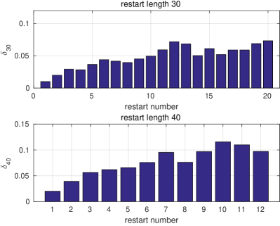
Figure 4: Residual convergence plot (left) and the values of $\delta_{k_{\max}}$ against the restart numbers (right) for the convection–diffusion test problem (see Section 3.1). The matrix $A$ is a discretized convection–diffusion operator for Peclet number $\textit{P\!e}=100$, mesh $102\times 102$ ($n=100^{2}$).

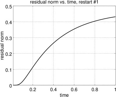
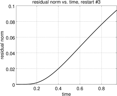
Figure 5: Residual norms $\|r_{k}(s)\|$ versus $s\in[0,t]$ at the end of the first (left) and the third (right) restart cycles of length 40 for the convection–diffusion test problem (see Section 3.1). The time interval at right is shorter, as it has been decreased at first two restarts. The matrix $A$ is a discretized convection–diffusion operator for Peclet number $\textit{P\!e}=100$, mesh $102\times 102$ ($n=100^{2}$).

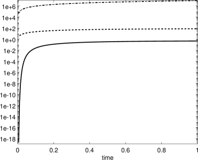
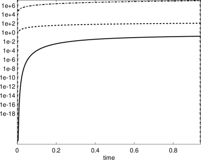
Figure 6: Residual norms $\|r_{k}(s)\|$ versus $s\in[0,t]$ (left and right, solid lines) as shown in Figure 5, together with their upper bounds given by Lemma 1 and estimates (16). Dashed lines: $h_{k+1,k}\|u(s)-u(0)\|$. Dashed–dotted and dotted lines (coinciding): $s\beta h_{k+1,k}\|H_{k}\|\,\|\varphi_{1}(-sH_{k})\|$ and $s\beta h_{k+1,k}\|H_{k}\||\varphi_{1}(-s\omega_{k})|$.

2.4 Making the restarting procedure adaptive

As can be seen in numerical experiments (see right plots in Figure 4), the value $\delta_{k_{\max}}$ tends to remain approximately constant after several first restarts. At each restart the time interval is decreased from $[0,t]$ to $[0,t-\delta_{k_{\max}}]$. Hence, at the end of each restart we can estimate the number of restarts that have yet to be done as $\approx t/\delta_{k_{\max}}$.

This observation allows to make our time restarting procedure adaptive as follows. Denote by $[\cdot]$ the rounding operation to the nearest integer. While carrying out Krylov steps $k=1,\dots,k_{\max}$, we compute for several values $k$ (in our experiments these are $[k_{\max}/3]$, $[2k_{\max}/3]$, $[5k_{\max}/6]$ and $k_{\max}$) the values $\delta_{k}$ and measured CPU times $t_{k}^{\mathsf{cpu}}$ spent to carry out these $k$ steps. Then the values

$$\dfrac{t}{\delta_{k}}t_{k}^{\mathsf{cpu}},\quad k=[k_{\max}/3],\;[2k_{\max}/3],\;[5k_{\max}/6],\;k_{\max}$$

are estimates of the remaining CPU needed to finish the computations for the restart lengths $[k_{\max}/3]$, $[2k_{\max}/3]$, $[5k_{\max}/6]$ and $k_{\max}$, respectively. Having computed these values during the restart, we can adjust the restart length for the next restart to have the smallest expected CPU time. In the experiments shown below we do so only if the expected gain in CPU time exceeds 5%. This adaptation procedure is then carried out at the end of every restart and also includes an option for an adaptive increase of the restart length as follows. If the current restart length is $\tilde{k}$, with $\tilde{k}<k_{\max}$, and the CPU time estimations indicate that the restart length $\tilde{k}$ is the optimal one then the new restart length is set to $\min\{\tilde{k}+5,k_{\max}\}$. We call this adaptive restarting ART: adaptive residual–time restarting. In Section 3 we test the ART restarting numerically and discuss it further.

2.5 RT restarting for the SAI Krylov subspace method

Shift-and-invert (SAI) Krylov subspace methods for computing actions of the matrix exponential are rational Krylov subspace methods designed to have a much faster convergence (in terms of the Krylov subspace dimension) than in regular polynomial Krylov subspace methods [30, 40]. In SAI methods the Krylov subspace is built up for the matrix $(I+\gamma A)^{-1}$, $\gamma>0$, rather than for $A$, and thus the price to pay for the faster convergence is solution, at each Krylov step, of linear systems with the matrix $I+\gamma A$. If these linear systems are solved by an iterative method, there are efficient strategies to save computational work by relaxing the tolerance to which the systems are solved [40]. The shift $\gamma$ can be chosen depending on the required tolerance $\mathtt{tol}$, and for the tolerances of order $10^{-5}$ to $10^{-7}$ a good value of $\gamma$ is $t/10$ where $t$ is the time interval length [40]. This is the value we use in all our experiments. An attractive property of the SAI Krylov methods is their often observed space–mesh independent convergence, which can be proven for the discretizations of parabolic PDEs with a numerical range close to the positive real axis [40, 16].

We now describe how the RT restarting strategy described above can be applied within the SAI Krylov subspace methods. The regular Arnoldi decomposition (4),(5) still holds for the SAI methods, namely

$$(I+\gamma A)^{-1}V_{k}=V_{k+1}\underline{\widetilde{H}}_{k}=V_{k}\widetilde{H}_{k}+\widetilde{h}_{k+1,k}v_{k+1}e_{k}^{T},$$ (17)

where $\widetilde{H}_{k}\in\mathbb{R}^{k\times k}$ denotes the first $k$ rows of $\underline{\widetilde{H}}_{k}$. The approximation $y_{k}(t)\approx\exp(-tA)v$ is computed according to (6), with $H_{k}$ being the SAI back transformed projection:

$$H_{k}=\frac{1}{\gamma}(\widetilde{H}_{k}^{-1}-I).$$ (18)

After rewriting the SAI Arnoldi decomposition (17) as [40, formula (4.1)]

$$AV_{k}=V_{k}H_{k}-\frac{\widetilde{h}_{k+1,k}}{\gamma}(I+\gamma A)v_{k+1}e_{k}^{T}\widetilde{H}_{k}^{-1},$$ (19)

we can see that the residual $r_{k}(t)=-y^{\prime}_{k}(t)-Ay_{k}(t)$ in the SAI Krylov subspace method reads [7]

$$r_{k}(t)=\beta_{k}(t)(I+\gamma A)v_{k+1},\qquad\beta_{k}(t)=\beta\,\frac{\widetilde{h}_{k+1,k}}{\gamma}\,e_{k}^{T}\widetilde{H}_{k}^{-1}\exp(-tH_{k})e_{1}.$$ (20)

This residual function $r_{k}(s)$ has quite a different dependence on $s\in[0,t]$ than the residual in the regular Krylov method (8): its convergence $\|r_{k}(s)\|\rightarrow 0$ with growing $k$ is much more uniform in $s\in[0,t]$. This means that we can not expect that $r_{k}(s)$ is much smaller in norm for small $s$ than for larger $s$. Typical dependence of the SAI residual norm $\|r_{k}(s)\|$ on $s\in[0,t]$ is shown in Figure 7.

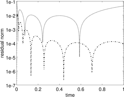
Figure 7: Residual norms $\|r_{k}(s)\|$ versus $s\in[0,t]$ of the SAI Krylov subspace method after $k=5$ (dotted line) and $k=10$ (dash-dotted line) Krylov steps for the convection–diffusion test problem (see Section 3.1). The matrix $A$ is a discretized convection–diffusion operator for Peclet number $\textit{P\!e}=100$, mesh $102\times 102$ ($n=100^{2}$).

As we see, there are a few distinct points $s$ on the interval $[0,t]$ where $\|r_{k}(s)\|$ has values much smaller than the average value $\frac{1}{t}\int_{0}^{t}\|r_{k}(s)\|\,ds$. Therefore, we can carry out the RT restarting procedure by assigning $\delta_{k}$ the value $s$ at which $\|r_{k}(s)\|$ has the smallest value:

$$\delta_{k}:=\arg\min_{s\in[0,t]}\|r_{k}(s)\|.$$

The rest of the RT restarting is carried out exactly in the same way as for regular Krylov subspace methods, i.e., we set $v:=y_{k_{\max}}(\delta_{k_{\max}})$ and proceed further by solving the IVP (2) on a shorter time interval $[0,t-\delta_{k_{\max}}]$. The drawback of this approach is that the reachable accuracy is restricted by the value $\|r_{k}(\delta_{k})\|=\min_{s\in[0,t]}\|r_{k}(s)\|$ (this is the error introduced to the initial data of the restarted IVP by setting $v:=y_{k_{\max}}(\delta_{k_{\max}})$). For instance, as can be seen in Figure 7, for the restart length $k_{\max}=5$ we have $\delta_{k}\approx 0.6$ and the reachable accuracy is $\min_{s\in[0,t]}\|r_{k}(s)\|\approx 10^{-5}$. In practical implementations of the method a warning should be given if such an accuracy drop takes place during the restart (i.e., if it turns out that $\min_{s\in[0,t]}\|r_{k}(s)\|$ is larger than the prescribed tolerance $\mathtt{tol}$). We further discuss the RT restarted SAI Krylov subspace methods in Section 3.

3 Numerical experiments

All the numerical tests are carried out on a Linux PC with 8 CPUs Intel Xeon E5504 2.00GHz in Matlab. No parallelization is carried out for the regular Arnoldi method. However, for Arnoldi/SAI methods automatic parallelization of the sparse LU factorizations is employed by Matlab.

3.1 Convection–diffusion test problem

In this test problem the matrix $A$ is a standard five point central-difference discretization of the following convection–diffusion operator acting on $u(x,y)$, defined for $(x,y)\in[0,1]\times[0,1]$ and satisfying the homogeneous Dirichlet boundary conditions:

$$L[u]=-(D_{1}u_{x})_{x}-(D_{2}u_{y})_{y}+\textit{P\!e}{}\,\left(\frac{1}{2}(v_{1}u_{x}+v_{2}u_{y})+\frac{1}{2}((v_{1}u)_{x}+(v_{2}u)_{y})\right)$$

$$D_{1}(x,y)=\begin{cases}10^{3}\;&(x,y)\in[0.25,0.75]^{2},\\ 1&\text{otherwise},\end{cases}\qquad\quad D_{2}(x,y)=\frac{1}{2}D_{1}(x,y),$$

$$v_{1}(x,y)=x+y,\qquad v_{2}(x,y)=x-y.$$

where the convective terms (i.e., the terms containing the first derivatives of $u$) are written in this specific form to guarantee that the contribution of the convection terms results in a skew-symmetric matrix [27]. In the experiments, we use matrices $A$ discretized on mesh $802\times 802$ for the Peclet number $\textit{P\!e}=200$ and on mesh $1202\times 1202$ for the Peclet number $\textit{P\!e}=300$. The problem size for these meshes is then $n=640\,000$ and $n=1\,440\,000$, respectively. In both cases $\|\frac{1}{2}(A+A^{T})\|_{2}\approx 6000$ and $\|\frac{1}{2}(A-A^{T})\|_{2}\approx 0.5$, so that the matrices are weakly non-symmetric. The initial vector $v$ is set to the values of the function $\sin(\pi x)\sin(\pi y)$ on the finite-difference mesh and then normalized as $v:=v/\|v\|$. The final time is set to $t=1$ and the tolerance to $\mathtt{tol}=10^{-6}$.

We compare the Krylov subspace method based on the Arnoldi process and our RT restarting with the following three methods:

1. The phiv function of the EXPOKIT package [35] based on the EXPOKIT time stepping restarting strategy.

2. Krylov subspace method based on the Arnoldi process and residual restarting [31, Chapter 3].

3. Krylov subspace method based on the Arnoldi process and NH (Niehoff–Hochbruck) restarting [31, Chapter 3].

We note that our implementations of the Arnoldi method do not include reorthogonalization of the Krylov basis vectors and we have not noticed a serious orthogonality loss. In the tables of this section presenting numerical results, the last two restarting methods are indicated by “Res” and “NH”, respectively. In these tables, the restarting methods presented in this paper are denoted by “RT” (residual–time) and “ART” (adaptive RT) restarting.

Table 1: Results for the convection–diffusion test problem. The restart ways are denoted by “Res” (residual based), “NH” (Niehoff–Hochbruck), “RT” (residual–time) and “ART” (adaptive RT). EXPOKIT uses time–stepping restarts.

method	restart	CPU	steps	error
	length, way	time, s
$\textit{P\!e}=200$, mesh $802\times 802$
EXPOKIT	30	57.3	800	3.82e-08
Arnoldi	30, Res	67.8	316	1.18e-07
Arnoldi	30, NH	71.7	317	1.02e-08
Arnoldi	30, RT	44.6	569	2.28e-08
Arnoldi	30, ART	41.1	572	2.05e-08
EXPOKIT	40	63.6	756	5.22e-09
Arnoldi	40, Res	74.9	298	4.40e-08
Arnoldi	40, NH	78.1	299	9.80e-09
Arnoldi	40, RT	45.1	505	1.18e-08
Arnoldi	40, ART	42.9	499	1.27e-08
$\textit{P\!e}=300$, mesh $1202\times 1202$
EXPOKIT	30	129.2	800	3.25e-08
Arnoldi	30, Res	136.9	310	8.34e-08
Arnoldi	30, NH	145.0	312	9.99e-09
Arnoldi	30, RT	90.7	539	2.83e-08
Arnoldi	30, ART	85.8	538	2.55e-08
EXPOKIT	40	147.3	756	4.09e-09
Arnoldi	40, Res	161.1	292	2.51e-08
Arnoldi	40, NH	154.2	293	1.08e-08
Arnoldi	40, RT	98.3	489	1.26e-08
Arnoldi	40, ART	93.7	492	1.01e-08

A simple way to restart Krylov subspace evaluations of the matrix exponential is to split the time interval into smaller intervals (time steps), on which the method converges within an acceptable number of Krylov steps. A question arises how this time-stepping restarting approach is compared to our RT restarting. To answer this question we include into comparisons the EXPOKIT package, which exploits such a time-stepping restarting [35].

The results of the comparisons are presented in Tables 1 and 2. The values reported there in the column “error” are relative error norms computed with respect to the EXPOKIT solution. The results in Table 1 show that our RT and ART restarting strategies outperform the other restarting strategies in terms of the CPU time. The residual based and NH restarting perform worse than the EXPOKIT restarting in terms of the CPU time. The reason for this is probably the sophisticated treatment of the projected problems in these restarting strategies, which creates an overhead in computational costs. Indeed, if, for instance, 5 restarts of length $k_{\max}=30$ are carried out with the NH restarting then the matrix exponential of a matrix size $150\times 150$ has to be computed. Additional costs in the residual based restarting is solution of a small projected ODE system, which, for this restarting, can not be solved by a matrix exponential evaluation [7]. Note also that the matrix-vector products are relatively cheap for this two-dimensional problems, which makes the other costs more pronounced.

In Table 2 the results for Arnoldi/SAI method are presented. In this case the method itself converges much quicker than the regular Arnoldi method, hence, fewer matrix–vector products are required and the restarting effects are less visible. However, we see that all the restarting strategies perform well in this case. The drawback of our RT restarting is that, as discussed in Section 2.5, it tends to deliver a less accurate solution for shorter restart lengths. We plan to address this problem in future.

Table 2: Results for the convection–diffusion test problem for the Arnoldi/SAI method. The restart ways are denoted by “Res” (residual based), “NH” (Niehoff–Hochbruck), “RT” (residual–time) and “ART” (adaptive RT). EXPOKIT uses time–stepping restarts.

method	restart	CPU	steps	error
	length, way	time, s
$\textit{P\!e}=200$, mesh $802\times 802$
Arnoldi/SAI	30, residual	46.8	16	1.35e-09
Arnoldi/SAI	30, NH	46.2	14	8.52e-09
Arnoldi/SAI	30, RT	44.7	14	8.52e-09
Arnoldi/SAI	10, residual	48.1	18	3.90e-07
Arnoldi/SAI	10, NH	45.4	14	1.24e-08
Arnoldi/SAI	10, RT	46.2	20	2.50e-07
Arnoldi/SAI	5, residual	54.5	20	1.08e-09
Arnoldi/SAI	5, NH	45.4	14	1.43e-08
Arnoldi/SAI	5, RT	43.8	13	4.25e-05
$\textit{P\!e}=300$, mesh $1202\times 1202$
Arnoldi/SAI	10, residual	159.8	17	2.58e-07
Arnoldi/SAI	10, NH	155.5	14	8.16e-09
Arnoldi/SAI	10, RT	154.3	14	8.03e-08
Arnoldi/SAI	5, residual	159.1	15	1.75e-07
Arnoldi/SAI	5, NH	155.5	14	8.31e-09
Arnoldi/SAI	5, RT	153.6	15	8.14e-06
$\textit{P\!e}=300$, mesh $1202\times 1202$, $t=10$
Arnoldi/SAI	30, Res	110.3	17	2.94e-09
Arnoldi/SAI	30, NH	108.0	15	1.25e-08
Arnoldi/SAI	30, RT	106.0	15	1.25e-08
Arnoldi/SAI	10, Res	109.5	18	1.42e-06
Arnoldi/SAI	10, NH	106.5	15	1.57e-08
Arnoldi/SAI	10, RT	104.0	15	1.57e-05

3.2 Photonic crystal test problem

This test problem is a space-discretized system of the three-dimensional Maxwell equations in a lossless and source-free medium:

$$\frac{\partial\bm{H}}{\partial t} =-\frac{1}{\mu}\nabla\times\bm{E},$$ (21)

$$\frac{\partial\bm{E}}{\partial t} =\frac{1}{\varepsilon}\nabla\times\bm{H},$$

where $\varepsilon$ and $\mu$ are scalar functions of $(x,y,z)$ representing permittivity and permeability, respectively, and $\bm{H}$ and $\bm{E}$ are vector-valued functions of $(x,y,z,t)$ representing unknown magnetic and electric fields, respectively. The boundary conditions are homogeneous Dirichlet. The spatial setup for this test problem is taken from the second test in [26]: in a spatial domain $[-6.05,6.05]\times[-6.05,6.05]\times[-6.05,6.05]$ filled with air (relative permittivity $\varepsilon_{r}=1$) there is a dielectric specimen occupying the region $[-4.55,4.55]\times[-4.55,4.55]\times[-4.55,4.55]$. The specimen has 27 spherical voids ($\varepsilon_{r}=1$) of radius $1.4$, whose centers have coordinates $(x_{i},y_{j},z_{k})=(3.03i,3.03j,3.03k)$, $i,j,k=-1,0,1$. The relative permittivity in the dielectric specimen is $\varepsilon_{r}=5.0$. The initial values are zero for all the components of both fields $\bm{H}$ and $\bm{E}$ except for the $x$- and $y$-components of $\bm{E}$: they are set to nonzero values in the middle of the spatial domain to represent a light emission. In addition, the initial value vector $v$ is normalized as $v:=v/\|v\|$. The standard finite-difference staggered Yee discretization in space leads to an ODE system of the form (2). The meshes $40\times 40\times 40$ and $80\times 80\times 80$ used in this test lead to problem size $n=413\,526$ and $n=3\,188\,646$, respectively. The final time is now set to $t=10$ and the tolerance to $\mathtt{tol}=10^{-6}$.

In the second test problem we compare the two solvers which come out as the best for the first test problem, namely the phiv solver of EXPOKIT [35] and our RT restarting (along with its adaptive version ART). Our experience reveals that the SAI strategy is inefficient in this test problem, which can be expected due to a strong nonsymmetry of $A$. This is in contrast to discretized Maxwell equations with nonreflecting boundary conditions or in lossy media, where SAI can be efficient [43, 6].

The results are presented in Table 3, where the values reported there in the column “error” are relative error norms computed with respect to the EXPOKIT solution. As we see, the RT restarting performs well comparably to EXPOKIT and outperforms it for longer restarts. We also see that the ART restarting, as expected, indeed helps to reduce the CPU time, possibly at the cost of the increased total number of Krylov steps.

Table 3: Results for the photonic crystal test problem. The restart ways are denoted by “RT” (residual–time) and “ART” (adaptive RT). EXPOKIT uses time–stepping restarts.

method	restart	CPU	steps	error
	length, way	time, s
mesh $40\times 40\times 40$
EXPOKIT	30	10.6	256	1.02e-06
Arnoldi	30, RT	11.3	231	5.19e-07
Arnoldi	30, ART	11.2	229	5.80e-07
EXPOKIT	70	23.3	288	2.16e-09
Arnoldi	70, RT	14.4	168	1.17e-07
Arnoldi	70, ART	14.4	167	1.57e-07
mesh $80\times 80\times 80$
EXPOKIT	30	155.2	512	4.37e-07
Arnoldi	30, RT	162.0	502	3.15e-07
Arnoldi	30, ART	160.8	488	4.06e-07
EXPOKIT	40	170.3	420	2.25e-06
Arnoldi	40, RT	160.8	427	2.77e-07
Arnoldi	40, ART	168.9	417	9.69e-07
EXPOKIT	50	178.9	416	2.33e-07
Arnoldi	50, RT	169.1	383	1.52e-07
Arnoldi	50, ART	169.1	379	2.31e-07
EXPOKIT	60	208.1	434	2.43e-08
Arnoldi	60, RT	181.3	354	1.06e-07
Arnoldi	60, ART	169.0	378	1.49e-07
EXPOKIT	70	250.5	432	2.74e-08
Arnoldi	70, RT	190.1	338	8.16e-08
Arnoldi	70, ART	162.2	389	1.06e-07

4 Conclusions and outlook

In this paper a new restarting RT (residual–time) procedure for Krylov subspace matrix exponential evaluations is proposed, analyzed and tested numerically. Our restarting is algorithmically simple as it only relies on evaluation of the readily available residual (8) and the restarted problem has the same form (2) as the original one. Furthermore, the RT restarting compares favorably to three other restarting techniques, namely, the time step restarting of EXPOKIT [35], the generalized residual restarting of Niehoff–Hochbruck [31] and the residual-based restarting [9, 7]. For the rational SAI (shift-and-invert) Krylov subspace approximations the proposed restarting works well for moderate accuracy requirements. The RT restarting is also implemented adaptively and the adaptive RT (ART) Krylov subspace method is available as a part of the Octave/Matlab package expmARPACK at http://team.kiam.ru/botchev/expm/.

Our future research plans include extension of this restarting approach to nonhomogeneous and nonlinear ODE systems, in combination with the exponential block Krylov method [5]. Furthermore, it would be interesting to see how this approach will work for second order ODE systems, where the matrix cosine and sine functions are involved.

The authors thank Vladimir Druskin for stimulating discussions.

References

- [1] M. Afanasjew, M. Eiermann, O. G. Ernst, and S. Güttel. Implementation of a restarted Krylov subspace method for the evaluation of matrix functions. Linear Algebra Appl., 429:2293–2314, 2008.
- [2] A. H. Al-Mohy and N. J. Higham. Computing the action of the matrix exponential, with an application to exponential integrators. SIAM J. Sci. Comput., 33(2):488–511, 2011. http://dx.doi.org/10.1137/100788860.
- [3] B. Beckermann. Image numérique, GMRES et polynômes de Faber. C. R. Acad. Sci. Paris: Ser. I, 340(11):855–860, 2005.
- [4] B. Beckermann and L. Reichel. Error estimation and evaluation of matrix functions via the Faber transform. SIAM J. Num. Anal., 47:3849–3883, 2009.
- [5] M. A. Botchev. A block Krylov subspace time-exact solution method for linear ordinary differential equation systems. Numer. Linear Algebra Appl., 20(4):557–574, 2013.
- [6] M. A. Botchev. Krylov subspace exponential time domain solution of Maxwell’s equations in photonic crystal modeling. J. Comput. Appl. Math., 293:24–30, 2016. http://dx.doi.org/10.1016/j.cam.2015.04.022.
- [7] M. A. Botchev, V. Grimm, and M. Hochbruck. Residual, restarting and Richardson iteration for the matrix exponential. SIAM J. Sci. Comput., 35(3):A1376–A1397, 2013. http://dx.doi.org/10.1137/110820191.
- [8] M. A. Botchev, G. L. G. Sleijpen, and H. A. van der Vorst. Stability control for approximate implicit time stepping schemes with minimum residual iterations. Appl. Numer. Math., 31(3):239–253, 1999.
- [9] E. Celledoni and I. Moret. A Krylov projection method for systems of ODEs. Appl. Numer. Math., 24(2-3):365–378, 1997.
- [10] H. De Raedt, K. Michielsen, J. S. Kole, and M. T. Figge. One-step finite-difference time-domain algorithm to solve the Maxwell equations. Phys. Rev. E, 67:056706, 2003.
- [11] K. Dekker and J. G. Verwer. Stability of Runge–Kutta methods for stiff non-linear differential equations. North-Holland Elsevier Science Publishers, 1984.
- [12] V. L. Druskin, A. Greenbaum, and L. A. Knizhnerman. Using nonorthogonal Lanczos vectors in the computation of matrix functions. SIAM J. Sci. Comput., 19(1):38–54, 1998.
- [13] V. L. Druskin and L. A. Knizhnerman. Two polynomial methods of calculating functions of symmetric matrices. U.S.S.R. Comput. Maths. Math. Phys., 29(6):112–121, 1989.
- [14] M. Eiermann and O. G. Ernst. A restarted Krylov subspace method for the evaluation of matrix functions. SIAM Journal on Numerical Analysis, 44:2481–2504, 2006.
- [15] M. Eiermann, O. G. Ernst, and S. Güttel. Deflated restarting for matrix functions. SIAM J. Matrix Anal. Appl., 32(2):621–641, 2011.
- [16] T. Göckler and V. Grimm. Uniform approximation of -functions in exponential integrators by a rational Krylov subspace method with simple poles. SIAM Journal on Matrix Analysis and Applications, 35(4):1467–1489, 2014. http://dx.doi.org/10.1137/140964655.
- [17] G. H. Golub and C. F. Van Loan. Matrix Computations. The Johns Hopkins University Press, Baltimore and London, third edition, 1996.
- [18] S. Güttel. Rational Krylov Methods for Operator Functions. PhD thesis, Technischen Universität Bergakademie Freiberg, March 2010. www.guettel.com.
- [19] S. Güttel, A. Frommer, and M. Schweitzer. Efficient and stable Arnoldi restarts for matrix functions based on quadrature. SIAM J. Matrix Anal. Appl, 35(2):661–683, 2014.
- [20] M. Hochbruck and C. Lubich. On Krylov subspace approximations to the matrix exponential operator. SIAM J. Numer. Anal., 34(5):1911–1925, Oct. 1997.
- [21] M. Hochbruck, C. Lubich, and H. Selhofer. Exponential integrators for large systems of differential equations. SIAM J. Sci. Comput., 19(5):1552–1574, 1998.
- [22] M. Hochbruck and A. Ostermann. Exponential integrators. Acta Numer., 19:209–286, 2010.
- [23] W. Hundsdorfer and J. G. Verwer. Numerical Solution of Time-Dependent Advection-Diffusion-Reaction Equations. Springer Verlag, 2003.
- [24] T. Jawecki, W. Auzinger, and O. Koch. Computable strict upper bounds for Krylov approximations to a class of matrix exponentials and -functions. arXiv preprint arXiv:1809.03369, 2018. https://arxiv.org/pdf/1809.03369.
- [25] L. A. Knizhnerman. Calculation of functions of unsymmetric matrices using Arnoldi’s method. U.S.S.R. Comput. Maths. Math. Phys., 31(1):1–9, 1991.
- [26] J. S. Kole, M. T. Figge, and H. De Raedt. Unconditionally stable algorithms to solve the time-dependent Maxwell equations. Phys. Rev. E, 64:066705, 2001.
- [27] L. A. Krukier. Implicit difference schemes and an iterative method for solving them for a certain class of systems of quasi-linear equations. Sov. Math., 23(7):43–55, 1979. Translation from Izv. Vyssh. Uchebn. Zaved., Mat. 1979, No. 7(206), 41–52 (1979).
- [28] V. I. Lebedev. Explicit difference schemes for solving stiff systems of ODEs and PDEs with complex spectrum. Russian J. Numer. Anal. Math. Modelling, 13(2):107–116, 1998.
- [29] I. Moret and P. Novati. An interpolatory approximation of the matrix exponential based on Faber polynomials. Journal of Computational and Applied Mathematics, 131(1-2):361–380, 2001.
- [30] I. Moret and P. Novati. RD rational approximations of the matrix exponential. BIT, 44:595–615, 2004.
- [31] J. Niehoff. Projektionsverfahren zur Approximation von Matrixfunktionen mit Anwendungen auf die Implementierung exponentieller Integratoren. PhD thesis, Mathematisch-Naturwissenschaftlichen Fakultät der Heinrich-Heine-Universität Düsseldorf, December 2006.
- [32] B. N. Parlett. The Symmetric Eigenvalue Problem. SIAM, 1998.
- [33] Y. Saad. Analysis of some Krylov subspace approximations to the matrix exponential operator. SIAM J. Numer. Anal., 29(1):209–228, 1992.
- [34] Y. Saad. Iterative Methods for Sparse Linear Systems. SIAM, 2d edition, 2003. Available from http://www-users.cs.umn.edu/~saad/books.html.
- [35] R. B. Sidje. Expokit. A software package for computing matrix exponentials. ACM Trans. Math. Softw., 24(1):130–156, 1998. www.maths.uq.edu.au/expokit/.
- [36] B. P. Sommeijer, L. F. Shampine, and J. G. Verwer. RKC: An explicit solver for parabolic PDEs. J. Comput. Appl. Math., 88:315–326, 1998.
- [37] P. K. Suetin. Series of Faber Polynomials. CRC Press, 1998.
- [38] H. Tal-Ezer. Polynomial approximation of functions of matrices and applications. Journal of Scientific Computing, 4(1):25–60, 1989.
- [39] H. Tal-Ezer. On restart and error estimation for Krylov approximation of . SIAM J. Sci. Comput., 29(6):2426–2441, 2007.
- [40] J. van den Eshof and M. Hochbruck. Preconditioning Lanczos approximations to the matrix exponential. SIAM J. Sci. Comput., 27(4):1438–1457, 2006.
- [41] H. A. van der Vorst. An iterative solution method for solving , using Krylov subspace information obtained for the symmetric positive definite matrix . J. Comput. Appl. Math., 18:249–263, 1987.
- [42] H. A. van der Vorst. Iterative Krylov methods for large linear systems. Cambridge University Press, 2003.
- [43] J. G. Verwer and M. A. Botchev. Unconditionally stable integration of Maxwell’s equations. Linear Algebra and its Applications, 431(3–4):300–317, 2009.