Is the composite fermion state of Graphene a doped Chern insulator?

Abstract

Graphene in the presence of a strong external magnetic field is a unique attraction for investigations of the fractional quantum Hall (fQH) states with odd and even denominators of the fraction. Most of the attempts to understand Graphene in the strong-field regime were made through exploiting the universal low-energy effective description of Dirac fermions emerging from the nearest-neighbor hopping model of electrons on a honeycomb lattice. We highlight that accounting for the next-nearest-neighbor hopping terms in doped Graphene can lead to a unique redistribution of magnetic fluxes within the unit cell of the lattice. While this affects all the fQH states, it has a striking effect at a half-filled Landau-level state: it leads to a composite fermion state that is equivalent to the doped topological Chern insulator on a honeycomb lattice. At energies comparable to the Fermi energy, this state possesses a Haldane gap in the bulk proportional to the next-nearest-neighbor hopping and density of dopants. We argue that this microscopically derived energy gap survives the projection to the lowest band. We also conjecture that the gap should be present in a microscopic theory giving the recently proposed particle-hole symmetric Dirac composite fermion scenario of the half-filled Landau-level. The proposed gap is lower than the chemical potential, and is predicted to be parametrically separated from the Dirac point in the latter description. Finally we conclude by proposing experiments to detect this gap; the associated boundary mode; and encourage cold-atom setups to test other predictions of the theory.

I Introduction

Since the discovery of the “$1/3$-plateau” in resistivity in the 2DEG Al-Ga-AsTsui et al. (1982), the fractional quantum Hall (fQH) effect has since intrigued the researchers. A multitude of states between filling fractions $\nu=0$ and $\nu=1$ of the lowest Landau level has been seen in 2DEGsKukushkin et al. (1999); Verdene et al. (2007) and Dirac systemsDean et al. (2011); Du et al. (2009); Bolotin et al. (2009); Ghahari et al. (2011); Feldman et al. (2012, 2013) with patterns consistent with $n/(pn\pm 1)$ (the Jain seriesJain (1989); where $p$ is an even integer and $n\in\{1,2,...\}$). The even denominator states are even more exotic displaying anyonic behaviorZibrov et al. (2017).

Besides the experimental progress, there have been significant contributions from the theoretical side. Major advancements were provided by the formulation of the variational wavefunction by LaughlinLaughlin (1983), the composite fermion theory by JainJain (1989, 2015), the Chern-Simon’s (CS) gauge theory of the fQHEZhang et al. (1989); Lopez and Fradkin (1991, 1995), topological order in fQHE statesWen (1995), effect of spin degree of freedomDavenport and Simon (2012), to name a few. The physics of even denominators were explored in the famous Halperin-Lee-Read (HLR) theory of the half-filled Landau levelHalperin et al. (1993); the Dirac composite fermionSon (2015); new field theoriesGoldman and Fradkin (2018); and the vortex metal stateYou (2018). The half-filled Landau level has itself been an intense subject of investigationSedrakyan and Raikh (2008); Sedrakyan and Chubukov (2009); Geraedts et al. (2016); Wang et al. (2017).

The composite fermion description of the fQH within HLR theory has been one of the most productive ones. Recently, it has been argued, however, that the HLR theory needs to be modified in order to capture the correct symmetry properties (particularly the particle-hole symmetry) of the low-energy effective theory describing the $\nu=1/2$ state. Motivated by these new advances, a question emerges whether the half-filled lowest Landau-level state exhibits universal properties irrespective the microscopic characteristics of the system and whether it represents a quantum criticality and a stable phase of matter with well defined low-energy quasiparticles. Experimentally it has been observed that when the amount of the disorder is small, the Hall resistivity exhibits a linear behavior near $\nu=1/2$ state as a function of the magnetic field, $B$, between Jain’s fractional quantum Hall series. This observation, together with the fact that Ohm resistivity is also finite and continuous, does guarantee stability of the compressible state. Although the theoretical microscopic derivation of the state with correct symmetry properties is still lacking, we side with the idea that there exists modification of the flux attachment within the HLR approach, that yields Son’s Dirac composite fermions. Basing on this idea, we will outline here novel properties of composite fermions which are independent of a particular form of the flux attachment. Hence we will apply HLR theory to describe our predictions, conjecturing that the same universal features will show up in any macroscopic derivation of Dirac composite fermions, which is not only confined to the lowest energy sector.

The HLR theory is a continuous microscopic theory based on formally exact flux attachment procedure, where the composite fermion quasiparticle is obtained upon attaching an even number magnetic flux quanta to an electron. To describe the $\nu=1/2$ state, one attaches just two fluxes followed by the flux smearing mean-field ansatz. In this way, the background magnetic field is ultimately canceled out yielding the HLR composite fermion sea as a “variational” ground state for the system with Chern-Simons gauge fluctuations around it.

When extending this logic to lattices one introduces a lattice Chern Simons theory and perform a mean field consistent with Gauss law constraints. One can then remain in the lattice pictureKumar et al. (2014); Sedrakyan et al. (2012, 2014); Sedrakyan et al. (2015a); Maiti and Sedrakyan (2019) or take leap and consider the continuum limit after performing the mean-field as in Refs. Sedrakyan et al., 2012, 2014; Sedrakyan et al., 2015a; Maiti and Sedrakyan, 2019. This latter approach is what we pursue in this work with the intention to arrive at an HLR-like theory after the mean-field. We explore what a CS flux distribution in a lattice may look like (with nearest and next-neighbor hoppings) and the corresponding continuum limit spectrum. While studies have looked into the effect of degeneracies on the fQH states in latticesSodemann and MacDonald (2014); Wu et al. (2015), some important considerations regarding the role of next nearest neighbor (nnn) hoppings and the flux distribution within a unit cell had been postponed to a future consideration. Here we make an attempt to account for these aspects in doped Graphene, and report a modification to the known results especially at half-filling of the lowest Landau level. Our first result is that at half-filling of the Landau level, we do expect composite fermions. However, one must contrast this inference from those made with naive expectations. One could argue that if we applied the HLR-idea to Graphene, the flux-detachment from the composite fermions would lead to a complete cancellation of the background magnetic field and thus the spectrum on the composite fermions should be identical to doped Graphene in zero field as shown in Fig. 1b. Our theory suggests that while the low energy excitations may seem similar to the naive HLR version, the spectrum of composite fermions has a non-trivial Haldane type gapHaldane (1988) in the bulk spectra, with a chiral edge mode around the sample, as shown in Fig. 1c. The essential physical property that distinguishes the naive application of HLR from out theory is the presence of the nnn hopping in Graphene (which is not negligibleCastro Neto et al. (2009); Kundu (2011)). We emphasize that this is not the Dirac-composite fermion theorySon (2015) where the postulate is that it is the correct theory of composite fermions formed in a system of electrons in the continuum model with parabolic dispersion.

$\begin{array}[]{cc}\includegraphics[width=216.81pt]{schema.eps}&\includegraphics[width=216.81pt]{schemb.eps}\\ \includegraphics[width=216.81pt]{schemc.eps}&\includegraphics[width=216.81pt]{schemd.eps}\end{array}$

Figure 1: (a) A schematic of the dispersion of electronic states in Graphene in zero field. (b) The spectrum of composite fermion states at half-filling condition based on naive application of HLR-type theory (uniform background field cancellation). (c) The composite fermion spectra based on this work. It consists of a bulk gap and an edge state. (d) Conjecture for how the Dirac composite fermion analog might look like. This is not addressed in this work. The inset represents the scenario for a parabolic band. $E_{F}$ is the Fermi level.

The second result we demonstrate is that in a generic fQH state there is a flux distribution within a unit cell arising from the external and the emergent CS fields. The former is uniformly distributed across the unit cell and we refer to this type of distribution as the Maxwell type. The latter results in a flux modulation within the unit cell which can be seen as a superposition of a Maxwell type component $\phi_{MW}$ (which contributes to the total flux through the unit cell), and an intra-unit cell component $\phi_{H}$ (which is only responsible for flux modulation and does not contribute to any net flux through the unit cell). The flux $\phi_{MW}$ is an orbital component that can be accounted for by minimal coupling of a gauge field (that is given by the 2+1D CS action), where as $\phi_{H}$ is an intra-unit cell property that should be accounted for independently in the resulting two-component Hamiltonian (the closest analogy would be the spin-field coupling of Dirac electrons in the relativistic theory of electron).

In what follows, we will derive the origin of $\phi_{H}$ and argue for its existence whenever there are internal hoppings within the unit cell. We will apply this general scheme to nnn Graphene at half filling and derive the effective low energy topological Hamiltonian for composite fermions and present the flux distributions for other filling fractions. We provide predictions for the gap in terms of the lattice parameters of Graphene and external field and motivate some cold atom setups to test our theory.

II Peierls’ substitution with nnn Graphene

The first intriguing observation is about the tight binding Hamiltonian for Graphene with nnn hoppings. This can be written in the momentum space as

$$H = -t\left(\begin{array}[]{cc}rT^{A}_{\mathbf{k}}&T_{\mathbf{k}}\\ T^{*}_{\mathbf{k}}&rT^{B}_{\mathbf{k}}\end{array}\right).$$ (3)

Here, $t$ and $rt$ denote the nn and nnn hopping amplitudes respectively, and

$$T^{A}_{\mathbf{k}}=T^{B}_{\mathbf{k}} = e^{i\mathbf{k}\cdot\mathbf{a}_{1}}+e^{i\mathbf{k}\cdot\mathbf{a}_{2}}+e^{i\mathbf{k}\cdot\mathbf{a}_{3}}~{}+~{}{\rm c.c.},$$

$$T_{\mathbf{k}} = e^{i\mathbf{k}\cdot\mathbf{e}_{1}}+e^{i\mathbf{k}\cdot\mathbf{e}_{2}}+e^{i\mathbf{k}\cdot\mathbf{e}_{3}},$$ (4)

where $\mathbf{e}_{1}=\frac{a}{\sqrt{3}}(\frac{\sqrt{3}}{2},\frac{-1}{2});~{}\mathbf{e}_{2}=\frac{a}{\sqrt{3}}(0,1),~{}\mathbf{e}_{3}=-\frac{a}{\sqrt{3}}(\frac{\sqrt{3}}{2},\frac{1}{2})$ (the translations from A to B atoms of Graphene), and $\mathbf{a}_{1}=a(1,0),~{}\mathbf{a}_{2}=a(\frac{1}{2},\frac{\sqrt{3}}{2}),~{}\mathbf{a}_{3}=a(\frac{1}{2},\frac{-\sqrt{3}}{2})$ (the lattice translation vectors), where $a$ is the lattice constant. Observe that $T^{A}_{\mathbf{k}}=T_{\mathbf{k}}T^{*}_{\mathbf{k}}-3$ and $T^{B}_{\mathbf{k}}=T^{*}_{\mathbf{k}}T_{\mathbf{k}}-3$. When an external field $\mathbf{B}$ is applied, one employs the Peierls’ substitution and either resorts to a Hofstadter like schemeHofstadter (1976) to obtain the spectrum, or performs an expansion of $H$ around a high symmetry point ($\mathbf{k}_{0}$) in the Brilliouin zone(BZ) where the chemical potential is expected to lie, in powers of $\delta\mathbf{k}=\mathbf{k}-\mathbf{k}_{0}$ and setting $\delta\mathbf{k}\rightarrow-i\partial_{\mathbf{r}}+e\mathbf{A}\equiv\mathbf{p}$, such that $\mathbf{\nabla}\times\mathbf{A}=\mathbf{B}$. We shall refer to this procedure as elongating the momentum $\mathbf{k}$.

This seemingly simple prescription has led to many useful results in many lattices including Graphene (with $r=0$). When $r\neq 0$, the first thing we note is that upon momentum elongation $\mathbf{k}\rightarrow\mathbf{k}_{0}+\mathbf{p}$, $T^{A}_{\mathbf{k}_{0}+\mathbf{p}}\neq T_{\mathbf{k}_{0}+\mathbf{p}}T^{*}_{\mathbf{k}_{0}+\mathbf{p}}-3$. This is because,

$$e^{i\mathbf{p}\cdot\mathbf{e}_{1}}e^{-i\mathbf{p}\cdot\mathbf{e}_{2}}=e^{i\mathbf{p}\cdot\mathbf{a}_{3}}e^{-i2\pi\phi_{B}/\phi_{0}},$$ (5)

where $\phi_{B}=Ba^{2}/4\sqrt{3}$, the flux through the small triangle in Fig. 2; and $\phi_{0}=2\pi/e$ the flux quantum ($\hbar=1$). One is thus left with a choice of using either $T^{A}_{\mathbf{k}_{0}+\mathbf{p}}$ or $T_{\mathbf{k}_{0}+\mathbf{p}}T^{*}_{\mathbf{k}_{0}+\mathbf{p}}-3$ in the Hamiltonian.

This ambiguity is removed by noting that the two choices reflect the two translations from $A\rightarrow A$: directly ($T^{A}_{\mathbf{k}}$) or via $B$ ($T_{\mathbf{k}}T^{*}_{\mathbf{k}}$), which must not commute as it encloses a flux $\phi_{B}$. The choice of $T_{\mathbf{k}_{0}+\mathbf{p}}T^{*}_{\mathbf{k}_{0}+\mathbf{p}}$ is consistent with $\phi_{B}=0$ and hence we can conclude that the correct choice is using $T^{A/B}_{\mathbf{k}_{0}+\mathbf{p}}$. In other words, to obtain a Maxwell type flux distribution in a lattice, the momentum elongation must be carried out on the translations corresponding to every allowed hop on the lattice. Carrying this procedure out and expanding the Hamiltonian around the $K$-point of Graphene [$\mathbf{k}_{0}=\frac{1}{a}(\frac{4\pi}{3},0)$] to $\mathcal{O}(p^{2})$, we find

$$H_{B}(\mathbf{r}) = -t\left[r\bar{p}^{2}\sigma_{0}-\bar{p}_{x}\sigma_{x}-\bar{p}_{y}\sigma_{y}\right],$$ (6)

where $\bar{p}_{i}\equiv\sqrt{3}ap_{i}/2$. This effective low energy Hamiltonian can be exactly solved. The energy spectrum is

$$\frac{E^{\pm}}{-t} = 2r\phi_{b}n\pm\sqrt{2\phi_{b}n+r^{2}\phi_{b}^{2}},$$ (7)

where $\phi_{b}\equiv 3\sqrt{3}e\phi_{B}$. The wavefunctions for the $A/B$ components for the quantum number $n$ with the gauge choice of $\mathbf{A}=-By\hat{\mathbf{x}}$ are: $\psi^{\pm}_{B}=\Phi_{n}(\mathbf{r})$, $\psi^{\pm}_{A}=\Phi_{n-1}(\mathbf{r})/(c\pm\sqrt{1+c^{2}})$, where $c=r\sqrt{\phi_{b}/2n}$, and

$$\Phi_{n}(\mathbf{r})=\frac{1}{\sqrt{2^{n}n!\sqrt{\pi}}}e^{ikx}e^{-\bar{y}^{2}/2}H_{n}(\bar{y}).$$ (8)

Here $\bar{y}\equiv(y-kl^{2}_{B})/l_{B}$, $\l^{2}_{B}=1/Be$, $k$ is a quantum number corresponding to translations along $x$, and $n\in\{1,2,...\}$. For $n=0$, we have $-E/t=r\phi_{b}$ and the wavefunction components are $\psi_{B}=\Phi_{0}(\mathbf{r})$ and $\psi_{A}=0$. At the $K^{\prime}$ point where $\mathbf{k}_{0}=\frac{1}{a}\left(\frac{-4\pi}{3},0\right)$, our low energy Hamiltonian is the same as $H_{B}$ but with $p_{x}\rightarrow-p_{x}$. This leads to the same spectrum however, $\psi^{K}_{B}\rightarrow\psi^{K^{\prime}}_{A}$ and $\psi^{K}_{A}\rightarrow-\psi^{K^{\prime}}_{B}$. Thus the $n=0$ landau level at $K^{\prime}$ point only has sublattice $A$ occupied. The presence of nnn affects the relative weights of the respective sublattices. It must be noted that the expansion to $\mathcal{O}(p^{2})$ is only valid for weak fields such that $\phi_{B}/\phi_{0}\ll 1$.

At finite $r$, there is an interesting situation that arises specifically when $\phi_{B}=\phi_{0}/6$ (see Fig. 2). The total flux through the unit cell is $\phi_{0}$ meaning the phase accumulation around the unit cell is $2\pi$ which restores the translation invariance to the lattice, although the internal hoppings still acquire a Peierls’ phase. The distribution of this phase is demonstrated in the appendix. The effective Hamiltonian (at $K$ point) is

$$H_{B}(\mathbf{r}) = -t\left[r\bar{k}^{2}\sigma_{0}-\bar{k}_{x}\sigma_{x}-\bar{k}_{y}\sigma_{y}+r\phi_{b}\sigma_{z}\right].$$ (9)

The spectrum is $-E^{\pm}/t=r\bar{k}^{2}\pm\sqrt{\bar{k}^{2}+r^{2}\phi_{b}^{2}}$, with a spectral gap of $2r\phi_{b}|t|$. At such a value of the external field the system becomes equivalent to the Haldane’s model for GrapheneHaldane (1988). Given the lattice constant of Graphene of $a=2.46\AA$, this phenomenon is expected to happen when $6\phi_{B}=\frac{\sqrt{3}}{2}Ba^{2}=\phi_{0}$, resulting in an unrealistic magnetic field of $B\approx 8\times 10^{4}$T. Below we will show that the Haldane’s model can be realized for composite fermions at much weaker fields. But before we make this connection, we describe how the CS field affects the lattice and the flux distribution within the unit cell.

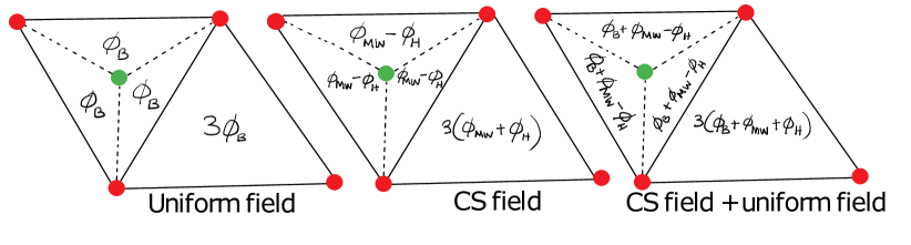
Figure 2: Flux distribution in a unit cell of Graphene in uniform external field, CS field, external$+$CS field. The CS field consists of a Maxwell part $\phi_{MW}$ and a modulated part $\phi_{H}$ ($=\phi_{MW}$) that does not contribute to the total flux. In the formulas we use the dimensionless fluxes $\phi_{b,h,mw}$ which are defined at appropriate places.

III The CS field in nnn Graphene

Consider a system of N particles with sets of coordinates $\{\mathbf{r}\}\equiv\{\mathbf{r}_{1},...,\mathbf{r}_{N}\}$. The many-body state $\Psi(\{\mathbf{r}\})$ constructed as a Slater determinant of the single particle states obeys $H_{\rm kin}(\{\mathbf{r}\})\Psi(\{\mathbf{r}\})=E\Psi(\{\mathbf{r}\})$ (where ‘kin’ denotes the kinetic part of the Hamiltonian). If the single particle states are picked from a manifold of degenerate states, one can propose another solution, without costing any energy, by introducing composite fermions in terms of original electrons coupled via a CS phase

$$\Psi(\{\mathbf{r}\})=e^{i\Lambda_{\{\mathbf{r}\}}}\Psi_{c}(\{\mathbf{r}\}),~{}\Lambda_{\{\mathbf{r}\}}=\kappa\sum_{\mathbf{r}^{\prime}\neq\mathbf{r}}\theta_{\mathbf{r}^{\prime}\mathbf{r}},$$ (10)

where $\theta_{\mathbf{r}^{\prime}\mathbf{r}}=\arg(\mathbf{r}^{\prime}-\mathbf{r})$, and $\kappa$ is an even integer to retain fermionic statistics of the resulting composite particles. It then follows that:

$$H(\{\mathbf{r}\})\Psi(\{\mathbf{r}\}) =E\Psi(\{\mathbf{r}\}),$$

$$\Rightarrow H(\{\mathbf{r}\},\mathbf{A}_{\{\mathbf{r}\}})\Psi_{c}(\{\mathbf{r}\}) =E\Psi_{c}(\{\mathbf{r}\}),$$

$${\rm MFA\Rightarrow} \left[\sum_{i}H_{\rm kin}(\mathbf{r}_{i},\mathbf{A}^{MW}_{\mathbf{r}_{i}})\right]\Psi^{\rm sl}_{c}(\{\mathbf{r}\}) =E\Psi^{\rm sl}_{c}(\{\mathbf{r}\}),$$ (11)

where $\mathbf{A}_{\{\mathbf{r}\}}(\mathbf{r}_{i})=\frac{1}{e}\partial_{\mathbf{r}_{i}}\Lambda_{\{\mathbf{r}\}}$; $H(\{\mathbf{r}\},\mathbf{A}_{\{\mathbf{r}\}})=e^{-i\Lambda_{\{\mathbf{r}\}}}H(\{\mathbf{r}\})e^{i\Lambda_{\{\mathbf{r}\}}}$; and ${\rm sl}$ stands for Slater determinant. The standard flux-smearing mean-field approximationHalperin et al. (1993) (MFA) designed to capture the transition to a topologically non-trivial system $H(\{\mathbf{r}\},\mathbf{A}_{\{\mathbf{r}\}})\rightarrow\sum_{\{\mathbf{r}\}}H_{\rm kin}(\mathbf{r},\mathbf{A}^{MW}_{\mathbf{r}})$. This amounts to changing the non-local $\mathbf{A}_{\{\mathbf{r}\}}$ to a local single-particle $\mathbf{A}^{MW}(\mathbf{r})$. Equivalently, the CS magnetic field defined by $\mathbf{B}(\mathbf{r})\equiv\nabla_{\mathbf{r}}\times\mathbf{A}_{\{\mathbf{r}\}}=\phi_{0}\kappa\sum_{\mathbf{r}^{\prime}\neq\mathbf{r}}\delta(\mathbf{r}^{\prime}-\mathbf{r})$ is approximated by a uniform $\mathbf{B}=\phi_{0}\kappa\rho_{2D}=\nabla_{\mathbf{r}}\times\mathbf{A}^{MW}_{\mathbf{r}}$. This is the many-body version of the field theories considered in Refs. Lopez and Fradkin (1991); Halperin et al. (1993). This formalism has been used in Refs. Sedrakyan et al. (2012, 2014); Sedrakyan et al. (2015a, b); Maiti and Sedrakyan (2019) to treat hard-core bosons as fermions with an odd $\kappa$ leading to chiral spin-liquid behaviour in honeycomb and Kagome lattices.

As discussed in Refs. Sedrakyan et al. (2014); Maiti and Sedrakyan (2019), the CS field produces a flux that is bound to a particle, the flux enclosed within the space of the particles in a unit cell must be zero. The net flux that arises from the MFA must then be re-distributed to the part of the unit cell that does not include any internal hoppings. Thus, the regions bounded by internal hoppings that are entirely within the unit cell (defined as loops having at the most one shared edge with external cells) must enclose zero flux. This is a constraint in our MFA to account for the CS character and distinguish it from a Maxwellian field. This constraint is efficiently implemented by introducing two types of fluxes: $\phi_{MW}$ (which contributes to the total flux per unit cell as constrained by the MFA) and $\phi_{H}$ (which does not contribute to the flux per unit cell). Our constraint requires $\phi_{H}=\phi_{MW}$ (see Fig. 2).

Note that this constraint implies that the direct $A\rightarrow A$ translation and the one mediated through a $B$ atom commute (which is different from the case of uniform field). Also note that while $\phi_{MW}$ can be accounted for by momentum elongation, $\phi_{H}$ cannot as it emerges as an internal degree of freedom due to the CS constraint. This results in the effective Hamiltonian (at the $K$ point) to be

$$H_{CS}(\mathbf{r}) = -t\left[r\bar{p}^{2}\sigma_{0}-\bar{p}_{x}\sigma_{x}-\bar{p}_{y}\sigma_{y}+r\phi_{h}\sigma_{z}\right],$$ (12)

where $\bar{\mathbf{p}}=\sqrt{3}a[-i\partial_{\mathbf{r}}+e\mathbf{A}^{MW}(\mathbf{r})]/2$, and $\phi_{h}=3\sqrt{3}e\phi_{H}$. Further, $[\bar{p}_{x},\bar{p}_{y}]=3\sqrt{3}\phi_{MW}$. Since the case of CS requires $\phi_{MW}=\phi_{H}$, it is possible to compact Eq. (12):

$$H_{CS}(\mathbf{r}) = -t\left[r\left\{\bar{\mathbf{p}}\cdot\mathbf{\sigma}\right\}^{2}-\bar{\mathbf{p}}\cdot\mathbf{\sigma}\right],$$ (13)

where the dot-product is 2-dimensional. Thus, $H_{CS}=-rt[H_{\mathbf{k}_{0}+\mathbf{p}}]^{2}-tH_{\mathbf{k}_{0}+\mathbf{p}}$. The CS nature of the field relates flux to density and requires that $\phi_{MW}=2\pi\kappa n_{uc}\nu_{l}/e$, where $n_{uc}$ is the number of atoms per unit cell and $\nu_{l}$ is the deviation from half-filling per site. The energy spectrum is:

$$\frac{E^{\pm}}{-t} = 2r|\phi_{mw}|n\pm\sqrt{2|\phi_{mw}|n},$$ (14)

where $\phi_{mw}=3\sqrt{3}e\phi_{MW}$, $n\in\{1,2,...\}$ and the wavefunctions are $\psi^{\pm}_{B}=\Phi_{n}(\mathbf{r})$, and $\psi^{\pm}_{A}=\pm\Phi_{n-1}(\mathbf{r})$. For $n=0$, $E=0$ and $\psi_{B}=\Phi_{0}(\mathbf{r})$ and $\psi_{A}=0$. At $K^{\prime}$ point $p_{x}\rightarrow-p_{x}$, $\phi_{h}\rightarrow-\phi_{h}$, and $\psi^{K}_{B}\rightarrow\psi^{K^{\prime}}_{A}$, $\psi^{K}_{A}\rightarrow-\psi^{K^{\prime}}_{B}$.

IV Composite Fermions in Graphene with nnn hoppings

The degenerate manifold that often motivates the use of the CS-phase attached to the many-body wavefunction can be thought of as being provided by an external field $\mathbf{B}$Halperin et al. (1993); Son (2015). We then have to account for three types of fluxes within the unit cell: $\phi_{B}$, $\phi_{MW}$ and $\phi_{H}$. As discussed, the first two produce a field that grows with area and can be accounted for by momentum elongation, while $\phi_{H}$ needs to be introduced at the level of matrix elements for the Hamiltonian (see appendix for detailed construction). The resulting theory is a fermion model populating Haldane’s model coupled to the CS action that was generated from flux attachment. This “statistical” CS term is the same as the one obtained in previous theories in the literatureZhang et al. (1989); Narevich et al. (2001). The distinguishing feature however is the flux distribution within the unit cell which is shown in Fig. 2. The resulting composite fermion(CF) Hamiltonian around the $K$-point is:

$$H_{\rm CF}(\mathbf{r})=-t\left[r\bar{p}^{2}\sigma_{0}-\bar{p}_{x}\sigma_{x}-\bar{p}_{y}\sigma_{y}+r\phi_{h}\sigma_{z}\right],$$ (15)

where $\mathbf{p}=-i\partial_{\mathbf{r}}+e\mathbf{A}^{B}_{\mathbf{r}}+e\mathbf{A}^{MW}_{\mathbf{r}}$, $\nabla_{\mathbf{r}}\times\mathbf{A}^{B}=\mathbf{B}$, which leads to the flux $\phi_{B}$, and $\nabla_{\mathbf{r}}\times\mathbf{A}^{MW}=\mathbf{B}^{MW}$ which leads to the flux $\phi_{MW}=\phi_{H}=\phi_{0}\kappa n_{uc}\nu_{l}$ from the induced CS field. Here $\kappa=-2~{}{\rm sgn}(B)$, where sgn($B$) simply indicates that the sign of $\kappa$ is such that the induced field opposes the external field. Just like in the HLR theory, the net ‘orbital’ field (resulting from the vector potential) experienced by the composite fermions is $\mathbf{B}_{\rm eff}=\mathbf{B}+\mathbf{B}^{MW}=\phi_{0}\rho_{2D}(1/\nu+\kappa)\hat{B}=\mathbf{B}(1-2\nu)$. But unlike the HLR theory, the two component nature of the lattice causes the composite fermions to experience an additional field that acts oppositely on the two atoms in the unit cell. This effect is captured by the flux $\phi_{H}$ and is analogous to the ‘spin’ coupling of the Maxwell field to the true spin-up/down fermions. The resulting spectrum is:

$$\frac{E^{\pm}}{-t}=2r|\phi_{b}+\phi_{mw}|n\pm\sqrt{2|\phi_{b}+\phi_{mw}|n+r^{2}\phi_{b}^{2}},$$ (16)

where $n\in\{1,2,...\}$, and for $n=0$ only $E^{+}$ is present. The wavefunctions are similar to the solutions for uniform field with $c\rightarrow\tilde{c}=r\sqrt{\phi_{b}/2n|1+\phi_{mw}/\phi_{b}|}$. Note that Eq. (15) is different from Eq. (12) in the definition of $\mathbf{p}$. Due to the presence of the external field, we cannot compact the Hamiltonian with a $(\mathbf{\sigma}\cdot\mathbf{p})^{2}$ term.

There are a number of points that need emphasis:(a) At half-filling ($\nu=1/2$), we have $\mathbf{B}_{\rm eff}=0$ and $\phi_{mw}=-\phi_{b}$. The spectrum of composite fermions is given by $E^{\pm}$ listed after Eq. (9) with the a spectral gap of $r\phi_{b}|t|$. (b) The resulting flux distribution in Fig. 2 at $\nu=1/2$ (with $\phi_{mw}=-\phi_{b}$) suggests that this is indeed the distribution considered by HaldaneHaldane (1988). (c) Just like the Landau-problem, Eq. (16) is to be seen as a solution to the composite fermions in a weak $\mathbf{B}_{\rm eff}$, which is realized by small departures from half-filling.

Noting that $\phi_{B}=\phi_{0}(n_{uc}\nu_{l})/6\nu$ and $\phi_{MW}=\phi_{0}(n_{uc}\nu_{l})\kappa/6$, treating $\phi_{B}$ and $\nu_{l}$ as external control variables, the $\nu=1/2$ condition is realized whenever $\nu_{l}$ and $\mathbf{B}$ satisfy $\phi_{0}\kappa(n_{uc}\nu_{l})=\sqrt{3}Ba^{2}/2$. Departures from $\nu=1/2$ can thus be achieved by slightly changing the field or $\nu_{l}$ (which can be achieved by changing the chemical potential). This mismatch creates the effective field that the composite fermions are subjected to. In fact, for small deviations such that $\phi_{b}=-\phi_{mw}+\delta$ ($\delta\ll\phi_{b}$), we get $-E^{\pm}/t\approx\pm r\phi_{b}(1\pm 2n|\delta|/\phi_{b})$.

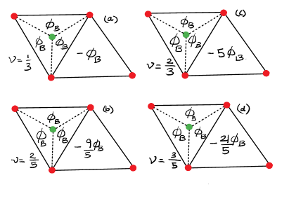
Figure 3: Flux distribution in a unit cell of Graphene for various fQHE states given by the Jain series.

We thus observe that the necessary characteristic of the composite fermion state in Graphene with nnn is the formation of the Haldane’s Chern insulator populated by composite fermions which, in turn, are coupled to the fluctuating “statistical” CS gauge field with the coefficient $\propto 1/4\pi\kappa$. The low-energy field theory description of this state is obtained upon integration over fermionic degrees of freedom. This results in an additional CS-like term, which combines with the statistical term resulting in a coefficient $\propto(1/4\pi\kappa+2\text{sgn}(B)/8\pi)\neq 0$ for the pure CS field. At this level, the low-energy description of the composite fermion state of Graphene does support an additional Chern-Simons action of the fluctuating field, by which it differs from the Dirac composite fermion construction by SonSon (2015) for a non-Dirac system. However, the low energy quasiparticles are still Dirac fermions, which is not surprising, since the original dispersion of electrons is not expected to qualitatively affect the ground state properties at very low energies because of complete quenching of the electronic kinetic energy by the strong magnetic field.

$\begin{array}[]{cc}\includegraphics[width=216.81pt]{Hoff1.eps}&\includegraphics[width=216.81pt]{Hoff2.eps}\end{array}$

Figure 4: The Hofstadter spectrum for a CS field acting on nnn Graphene with $r=0.11$ (left) and $r=0.22$ (right). Observe the linear scaling and the flatness of the lowest energy level in the two plots.

This prescription also works for any other fQHE state. Consider the Jain series: $\nu=n/(2n+1)$ and $\nu=(n+1)/(2n+1)$. It is easy to see that the total flux through the unit cell is given by $6(\phi_{B}+\phi_{MW})$. However, as discussed earlier, this flux is distributed as $\phi_{B}$ in each of the smaller triangles and $3(\phi_{B}+2\phi_{MW}$) in the larger triangle. Further, recall that $\phi_{MW}=\kappa\phi_{0}=-2\phi_{0}$, and $\phi_{B}=\phi_{0}/\nu$. Expressing everything in terms of $\phi_{B}$, the flux that is generated by the external magnetic field, the flux through the smaller triangles is always $\phi_{B}$, though the larger triangle is $3\phi_{B}(1-4\nu)$, and through the unit cell is $6\phi_{B}(1-2\nu)$. The resulting flux distributions for some of the fQHE states in the Jain series are shown in Fig. 3. The low energy Hamiltonian for small deviations around each $n$ can be derived by appropriately enlarging the unit-cell (as in the original Hofstadter constructionHofstadter (1976)): with the special care that $\phi_{H}$ has to be accounted for every matrix element of the Hamiltonian for the enlarged unit cell. A quantitative account of such flux modulation and its effect on the many-body wavefunction remains an open question that will provide a valuable information on Jain’s states.

V Experimental consequences

Our theory suggests that in addition to the expected Fermi-surface(FS), we must see a spectral gap in the bulk consistent with the Haldane’s model (Fig 1b). Following the formulas in the text, for a density of $\rho_{2D}=\bar{\rho}\times 10^{11}$cm^-2, this gap is $\approx r\bar{\rho}|t|$ meV (where $t$ must be in eV); and this happens at a $B\approx 8\bar{\rho}$ T. In Graphene, $t\approx 3$ eV and $r\sim 0.1$Castro Neto et al. (2009). If $\bar{\rho}$ is tuned from $1-10$, then for $B\sim 8$-$80$T, we should see a Haldane gap of $0.3$-$3$ meV. Further, $v\approx 1\times 10^{6}$ms^-1 implies $E_{F}\approx 8\sqrt{\bar{\rho}}$ meV which will range from $8$-$24$meV. The energy scale suggests that the Haldane gap can be probed by LDOS measurements via STM. Due to correspondence with Haldane’s model, the composite fermion bands are topological with Chern number $\pm 1$ and thus have chiral edge states which can be measured via tunneling into the edge Shytov et al. (1998); Ström and Johannesson (2009); Kamenev and Gefen (2015) and via measuring the quantized thermal transport due to a Luttinger liquid description of edge statesKane and Fisher (1997); Fern et al. (2018). The presence of a gapped spectrum for $\nu=1/2$ state in Graphene is in line with findings in the two component AlAsZhu et al. (2018).

V.1 Implication for cold atoms

There is an interesting consequence of our theory when applied to fermionic/bosonic cold atoms at low densities. When the nnn hopping is present ($r\neq 0$), a characteristic feature at $r=1/6$ distinguishes the flux distribution in our theory from those that might be predicted by other theories: when $r>1/6$, the minimum of the lattice spectrum in the presence of the external field (which forms from states around the $\Gamma$-point of the original system), is non-dispersive as shown in Fig. 4.

To understand this, consider the $\Gamma$-point the effective low energy Hamiltonian:

$$H^{\Gamma}=-t\left(\begin{array}[]{cc}r(9-2\bar{p}^{2})&3-\frac{1}{3}\bar{p}^{2}\\ 3-\frac{1}{3}\bar{p}^{2}&r(9-2\bar{p}^{2})\end{array}\right).$$ (17)

The spectrum is given by

$$\frac{E^{\pm}}{-t}=9r\pm 3-2\left(r\pm\frac{1}{6}\right)(2n+1)\phi_{b},$$ (18)

and the wavefunctions are $\psi^{\pm}_{A}=\pm\psi^{\pm}_{B}=\Phi_{n}(\mathbf{r})$, with $n\in\{0,1,2,...\}$. Thus for $r<1/6$, the energy of the lowest landau level, which can occur at any $n$, linearly increases with field. However, for $r>1/6$, the spectrum in Eq. (18) suggests that the energy goes down. This is indeed what happens for the uniform field case. However, for the CS case with $r>1/6$, the minimum of the energy for any $\{n,\phi_{mw}\}$ is actually locked at $E=-|t|/4r$. This means that the lowest energy level of the spectrum is dispersionless with the field $\phi_{b}$. This is not evident from Eq. (18) due to the fact that we expanded to $\mathcal{O}(p^{2})$.

This minimum is guaranteed because the Hamiltonian is of the form $rG^{2}_{\mathbf{p}}+G_{\mathbf{p}}$. This means the eigenvectors of $G_{\mathbf{p}}$ are also the eigenvectors of $G^{2}_{\mathbf{p}}$, with squared eigenvalues. The quadratic form suggests that there is a minimum of the energy for any eigenvalue. For $r<1/6$, this minimum energy scales with the field as $E=(1/6-r)\phi_{b}$, but for $r>1/6$ the minimum is at $E=t/4r$ for infinite pairs of $\{n,\phi_{mw}\}$. Note that this effect of CS field also applies to the $K/K^{\prime}$ point analysis. This we should expect a dispersionless band around the center of the spectrum. These cases are demonstrated in Fig. 4. In other words, if we were to tune $r$, our theory would predict that the lowest band in the plot for $E(\phi)$ will have a slope that decreases as $r$ increases and stall at zero slope (dispersionless). In other flux distributions, the slope becomes negative.

VI Concluding remarks

To summarize, we showed that Graphene with nnn hoppings near half-filling is described by a model of composite fermions living on Haldane’s Chern insulator model of Graphene. This perspective not only provides an internal flux distributions within the unit cell but also the effective wavefunctions for fQH states. Very interestingly, this perspective when applied to fermionization of bosons in flat bands (as done in Ref. Maiti and Sedrakyan, 2019), leads to chiral-spin liquid behavior. Thus besides motivating experiments, this work potentially provides a unified picture of treating chiral spin-liquids in spin-systems and fQH states in fermionic systems. We believe that this motivates further research and exploration of other fractional Quantum Hall systems along similar lines to compare and contrast with existing literature and guide future experiments.

At this stage one may ask the question: why are we doing an HLR type flux attachment instead of building a Dirac composite fermionSon (2015) analog? While we don’t directly answer this question, we point out that both HLR theory and the Dirac composite fermion theories ultimately give the same result for the observables. Since the bulk gap predicted in out theory is in principle an observable, we expect this result to be robust. The main reason we did not attempt the Dirac composite fermion analog is that it is necessarily limited to the low energy excitations and does not immediately address the presence of such a bulk gap. However, the topological properties of the chiral bands must be reproduced is such an approach and is an interesting question to address next.

Appendix A Peierls phases for uniform and Chern Simons’ fields

For definiteness, we shall work in the symmetric gauge where $\mathbf{A}(\mathbf{r})=(-y\hat{\mathbf{x}}+x\hat{\mathbf{y}})B/2$. The phase accumulated on a bond upon traversing in the direction $\mathbf{g}_{n}$ is given by $\bar{A}_{g_{n}}\equiv\int_{\mathbf{g}_{n}}\mathbf{A}\cdot d\mathbf{l}$. In the lattice problem, we may treat $\mathbf{A}$ to be constant for a unit translation of $\mathbf{g}_{n}$, where $\mathbf{g}_{n}\in\{\mathbf{e}_{1,2,3},\mathbf{a}_{1,2,3}\}$. The directions of these vectors are illustrated in Fig. 5. This leads to $\bar{A}_{g_{n}}=A_{g_{n}}+(-yg_{x}+xg_{y})Ba/2$, where $A_{g_{n}}$ refers to phase accumulation that can be gauged out and is the same contribution from every lattice point. Thus, $A_{e_{1}}+A_{e_{3}}+A_{e_{3}}=0$ and $A_{a_{1}}=A_{a_{2}}+A_{a_{3}}$. Once an origin is picked, we can start assigning $\bar{A}^{a/b}$ to denote phase accumulation originating from atom $a/b$ of the lattice. Thus for a given bond along $\mathbf{g}_{n}$, the phase can be written as $\bar{A}_{g_{n}}=\bar{A}^{a/b}_{g_{n}}+\Delta\bar{A}_{g_{n}}$, where $\bar{A}^{a/b}_{g_{n}}$ denotes the value of the bond at the origin, and $\Delta\bar{A}_{g_{n}}$ denotes the value at a bond separated from the origin by $(\Delta x,\Delta y)$. These quantities are expressed as (in the symmetric gauge):

$$\Delta\bar{A}_{a_{1}} = -\phi_{MW}\left(\frac{2\sqrt{3}\Delta y}{a}\right),$$ (19)

$$\Delta\bar{A}_{a_{2}} = \phi_{MW}\left(\frac{3\Delta x}{a}-\frac{\sqrt{3}\Delta y}{a}\right),$$ (20)

$$\Delta\bar{A}_{a_{3}} = -\phi_{MW}\left(\frac{3\Delta x}{a}+\frac{\sqrt{3}\Delta y}{a}\right),$$ (21)

$$\Delta\bar{A}_{e_{1}} = -\phi_{MW}\left(\frac{\Delta x}{a}+\frac{\sqrt{3}\Delta y}{a}\right),$$ (22)

$$\Delta\bar{A}_{e_{2}} = \phi_{MW}\left(\frac{2\Delta x}{a}\right),$$ (23)

$$\Delta\bar{A}_{e_{3}} = -\phi_{B}\left(\frac{\Delta x}{a}-\frac{\sqrt{3}\Delta y}{a}\right).$$ (24)

To initialize the bonds starting from the $a/b$ atoms belonging to the lattice point at the origin:

$$\bar{A}^{a}_{a_{1}} = A_{a_{1}}+\phi_{H},$$ (25)

$$\bar{A}^{a}_{a_{2}} = A_{a_{2}}-\phi_{H},$$ (26)

$$\bar{A}^{a}_{a_{3}} = A_{a_{3}}-\phi_{H},$$ (27)

$$\bar{A}^{b}_{a_{1}} = A_{a_{1}}+\phi_{MW}-\phi_{H},$$ (28)

$$\bar{A}^{b}_{a_{2}} = A_{a_{2}}+2\phi_{MW}+\phi_{H},$$ (29)

$$\bar{A}^{b}_{a_{3}} = A_{a_{3}}-\phi_{MW}+\phi_{H},$$ (30)

$$\bar{A}^{b}_{e_{1}} = A_{e_{1}},$$ (31)

$$\bar{A}^{b}_{e_{2}} = A_{e_{2}}+\phi_{MW},$$ (32)

$$\bar{A}^{b}_{e_{3}} = A_{e_{3}}-\phi_{MW}.$$ (33)

And finally $A_{g_{n}}\equiv\mathbf{A}^{\prime}\cdot\mathbf{g}_{n}$, where $\mathbf{A}^{\prime}$ is some vector which will be gauged out and can be set to zero for our purposes. The extended scheme is summarized in Fig. 5. Note that any field that grows with area will be treated as $\phi_{MW}$ and the internal modulation will be treated as $\phi_{H}$.

$\begin{array}[]{c}\includegraphics[width=346.89731pt]{A_atom}\\ \includegraphics[width=346.89731pt]{B_atom}\end{array}$

Figure 5: Extended scheme outlining the phase accumulation in addition to $\int\mathbf{A}\cdot d\mathbf{l}$ along each bond. The field $\mathbf{A}$ is written in symmetric gauge. The figure is split into $(a)$ and $(b)$ for clarity. The flux $\phi_{MW}$ adds up with area, whereas the flux $\phi_{H}$ denotes flux modulation within the unit cell such that net contribution from $\phi_{H}$ to the unit cell is zero. The presence of $\phi_{H}$ does not break translational symmetry.

Appendix B Effective Hamiltonians

Following the prescription in the above section, we are able to assign the phases to every matrix element involved in the Hamiltonian. The Hamiltonian of nearest neighbor Graphene in an external field can be derived from the lattice Hamiltonian as $H\rightarrow H_{B}$ where

$$H^{11}_{B} = r\left\{3+2\left[\cos(k_{0,1}-k_{0,2}+p_{1}-p_{2})\right.\right.$$

$$~{}~{}+\cos(k_{0,2}-k_{0,3}+p_{2}-p_{3})$$

$$\left.\left.+\cos(k_{0,3}-k_{0,1}+p_{3}-p_{1})\right]\right\},$$

$$H^{22}_{B} = r\left\{3+2\left[\cos(k_{0,1}-k_{0,2}+p_{1}-p_{2})\right.\right.$$

$$~{}~{}+\cos(k_{0,2}-k_{0,3}+p_{2}-p_{3})$$

$$\left.\left.+\cos(k_{0,3}-k_{0,1}+p_{3}-p_{1})\right]\right\},$$

$$H^{12}_{B} = T_{\mathbf{k}_{0}+\mathbf{p}},$$

$$H^{21}_{B} = T^{*}_{\mathbf{k}_{0}+\mathbf{p}},$$ (34)

where $x_{i}\equiv\mathbf{x}\cdot\mathbf{e}_{i}$, $\mathbf{k}_{0}$ is a point about which the semi-classical momentum elongation is carried out. It is understood that $H_{B}$ is to be expanded to $\mathcal{O}(p^{2})$. Here the elongated momentum $vp$ involves $\mathbf{A}^{B}$ such that $\mathbf{\nabla}\times\mathbf{A}^{B}=\mathbf{B}$.

When we consider the case of a Chern-Simons’(CS) field, we have to account for $\phi_{H}$. The Hamiltonian matrix elements look like

$$H^{11}_{CS} = r\left\{3+2\left[\cos(k_{0,1}-k_{0,2}+p_{1}-p_{2}-e\phi_{H})\right.\right.$$

$$~{}~{}+\cos(k_{0,2}-k_{0,3}+p_{2}-p_{3}-e\phi_{H})$$

$$\left.\left.+\cos(k_{0,3}-k_{0,1}+p_{3}-p_{1}-e\phi_{H})\right]\right\},$$

$$H^{22}_{CS} = r\left\{3+2\left[\cos(k_{0,1}-k_{0,2}+p_{1}-p_{2}+e\phi_{H})\right.\right.$$

$$~{}~{}+\cos(k_{0,2}-k_{0,3}+p_{2}-p_{3}+e\phi_{H})$$

$$\left.\left.+\cos(k_{0,3}-k_{0,1}+p_{3}-p_{1}+e\phi_{H})\right]\right\},$$

$$H^{12}_{CS} = T_{\mathbf{k}_{0}+\mathbf{p}},$$

$$H^{21}_{CS} = T^{*}_{\mathbf{k}_{0}+\mathbf{p}}.$$ (35)

Here the elongated momentum $vp$ involves $\mathbf{A}^{MW}$ such that $\mathbf{\nabla}\times\mathbf{A}^{MW}=\mathbf{B}_{MW}$. Note also that the $a/b$ atoms experience different signs of the flux $\phi_{H}$ although they originate from the same field $\mathbf{A}^{MW}$.

To address the HLR case, we have to account for the external field and the CS field. This results in a very similar looking Hamiltonian as in Eq. (B) but with $\mathbf{p}$ containing $\mathbf{A}^{B}$ and $\mathbf{A}^{MW}$, and $\phi_{H}$ is still only generated from $\mathbf{A}^{MW}$. The flux $\phi_{B}$ is generated from $\mathbf{A}^{B}$ and the flux $\phi_{MW}$ is generated from $\mathbf{A}^{MW}$.

When $\phi_{b}=-\phi_{mw}=\phi_{h}$, we realize the Haldane’s model of flux distribution in the unit cell. The extended scheme of the flux distribution shown in Fig. 1 of the main text (MT), is shown in Fig. 6 in this text.

Figure 6: The flux distribution arising from CS field in Graphene with next nearest neighbor hopping. The shaded region denotes the region of non-zero flux.

References

- Tsui et al. (1982) D. C. Tsui, H. L. Stormer, and A. C. Gossard, Phys. Rev. Lett. 48, 1559 (1982), URL https://link.aps.org/doi/10.1103/PhysRevLett.48.1559.
- Kukushkin et al. (1999) I. V. Kukushkin, K. v. Klitzing, and K. Eberl, Phys. Rev. Lett. 82, 3665 (1999), URL https://link.aps.org/doi/10.1103/PhysRevLett.82.3665.
- Verdene et al. (2007) B. Verdene, J. Martin, G. Gamez, J. Smet, K. von Klitzing, D. Mahalu, D. Schuh, G. Abstreiter, and A. Yacoby, Nature Physics 3, 392 EP (2007), URL https://doi.org/10.1038/nphys588.
- Dean et al. (2011) C. R. Dean, A. F. Young, P. Cadden-Zimansky, L. Wang, H. Ren, K. Watanabe, T. Taniguchi, P. Kim, J. Hone, and K. L. Shepard, Nature Physics 7, 693 EP (2011), URL https://doi.org/10.1038/nphys2007.
- Du et al. (2009) X. Du, I. Skachko, F. Duerr, A. Luican, and E. Y. Andrei, Nature 462, 192 EP (2009), URL https://doi.org/10.1038/nature08522.
- Bolotin et al. (2009) K. I. Bolotin, F. Ghahari, M. D. Shulman, H. L. Stormer, and P. Kim, Nature 462, 196 EP (2009), URL https://doi.org/10.1038/nature08582.
- Ghahari et al. (2011) F. Ghahari, Y. Zhao, P. Cadden-Zimansky, K. Bolotin, and P. Kim, Phys. Rev. Lett. 106, 046801 (2011), URL https://link.aps.org/doi/10.1103/PhysRevLett.106.046801.
- Feldman et al. (2012) B. E. Feldman, B. Krauss, J. H. Smet, and A. Yacoby, Science 337, 1196 (2012), ISSN 0036-8075, eprint http://science.sciencemag.org/content/337/6099/1196.full.pdf, URL http://science.sciencemag.org/content/337/6099/1196.
- Feldman et al. (2013) B. E. Feldman, A. J. Levin, B. Krauss, D. A. Abanin, B. I. Halperin, J. H. Smet, and A. Yacoby, Phys. Rev. Lett. 111, 076802 (2013), URL https://link.aps.org/doi/10.1103/PhysRevLett.111.076802.
- Jain (1989) J. K. Jain, Phys. Rev. Lett. 63, 199 (1989), URL https://link.aps.org/doi/10.1103/PhysRevLett.63.199.
- Zibrov et al. (2017) A. A. Zibrov, C. Kometter, H. Zhou, E. M. Spanton, T. Taniguchi, K. Watanabe, M. P. Zaletel, and A. F. Young, Nature 549, 360 EP (2017), URL https://doi.org/10.1038/nature23893.
- Laughlin (1983) R. B. Laughlin, Phys. Rev. Lett. 50, 1395 (1983), URL https://link.aps.org/doi/10.1103/PhysRevLett.50.1395.
- Jain (2015) J. K. Jain, Annual Review of Condensed Matter Physics 6, 39 (2015), eprint https://doi.org/10.1146/annurev-conmatphys-031214-014606, URL https://doi.org/10.1146/annurev-conmatphys-031214-014606.
- Zhang et al. (1989) S. C. Zhang, T. H. Hansson, and S. Kivelson, Phys. Rev. Lett. 62, 82 (1989), URL https://link.aps.org/doi/10.1103/PhysRevLett.62.82.
- Lopez and Fradkin (1991) A. Lopez and E. Fradkin, Phys. Rev. B 44, 5246 (1991), URL https://link.aps.org/doi/10.1103/PhysRevB.44.5246.
- Lopez and Fradkin (1995) A. Lopez and E. Fradkin, Phys. Rev. B 51, 4347 (1995), URL https://link.aps.org/doi/10.1103/PhysRevB.51.4347.
- Wen (1995) X.-G. Wen, Advances in Physics 44, 405 (1995), ISSN 0001-8732, URL https://doi.org/10.1080/00018739500101566.
- Davenport and Simon (2012) S. C. Davenport and S. H. Simon, Phys. Rev. B 85, 245303 (2012), URL https://link.aps.org/doi/10.1103/PhysRevB.85.245303.
- Halperin et al. (1993) B. I. Halperin, P. A. Lee, and N. Read, Phys. Rev. B 47, 7312 (1993), URL https://link.aps.org/doi/10.1103/PhysRevB.47.7312.
- Son (2015) D. T. Son, Phys. Rev. X 5, 031027 (2015), URL https://link.aps.org/doi/10.1103/PhysRevX.5.031027.
- Goldman and Fradkin (2018) H. Goldman and E. Fradkin, Phys. Rev. B 98, 165137 (2018), URL https://link.aps.org/doi/10.1103/PhysRevB.98.165137.
- You (2018) Y. You, Phys. Rev. B 97, 165115 (2018), URL https://link.aps.org/doi/10.1103/PhysRevB.97.165115.
- Sedrakyan and Raikh (2008) T. A. Sedrakyan and M. E. Raikh, Phys. Rev. B 77, 115353 (2008), URL https://link.aps.org/doi/10.1103/PhysRevB.77.115353.
- Sedrakyan and Chubukov (2009) T. A. Sedrakyan and A. V. Chubukov, Phys. Rev. B 79, 115129 (2009), URL https://link.aps.org/doi/10.1103/PhysRevB.79.115129.
- Geraedts et al. (2016) S. D. Geraedts, M. P. Zaletel, R. S. K. Mong, M. A. Metlitski, A. Vishwanath, and O. I. Motrunich, Science 352, 197 (2016), ISSN 0036-8075, eprint http://science.sciencemag.org/content/352/6282/197.full.pdf, URL http://science.sciencemag.org/content/352/6282/197.
- Wang et al. (2017) C. Wang, N. R. Cooper, B. I. Halperin, and A. Stern, Phys. Rev. X 7, 031029 (2017), URL https://link.aps.org/doi/10.1103/PhysRevX.7.031029.
- Kumar et al. (2014) K. Kumar, K. Sun, and E. Fradkin, Phys. Rev. B 90, 174409 (2014), URL https://link.aps.org/doi/10.1103/PhysRevB.90.174409.
- Sedrakyan et al. (2012) T. A. Sedrakyan, A. Kamenev, and L. I. Glazman, Phys. Rev. A 86, 063639 (2012), URL https://link.aps.org/doi/10.1103/PhysRevA.86.063639.
- Sedrakyan et al. (2014) T. A. Sedrakyan, L. I. Glazman, and A. Kamenev, Phys. Rev. B 89, 201112 (2014), URL https://link.aps.org/doi/10.1103/PhysRevB.89.201112.
- Sedrakyan et al. (2015a) T. A. Sedrakyan, L. I. Glazman, and A. Kamenev, Phys. Rev. Lett. 114, 037203 (2015a), URL https://link.aps.org/doi/10.1103/PhysRevLett.114.037203.
- Maiti and Sedrakyan (2019) S. Maiti and T. Sedrakyan, Phys. Rev. B 99, 174418 (2019), URL https://link.aps.org/doi/10.1103/PhysRevB.99.174418.
- Sodemann and MacDonald (2014) I. Sodemann and A. H. MacDonald, Phys. Rev. Lett. 112, 126804 (2014), URL https://link.aps.org/doi/10.1103/PhysRevLett.112.126804.
- Wu et al. (2015) F. Wu, I. Sodemann, A. H. MacDonald, and T. Jolicoeur, Phys. Rev. Lett. 115, 166805 (2015), URL https://link.aps.org/doi/10.1103/PhysRevLett.115.166805.
- Haldane (1988) F. D. M. Haldane, Phys. Rev. Lett. 61, 2015 (1988), URL https://link.aps.org/doi/10.1103/PhysRevLett.61.2015.
- Castro Neto et al. (2009) A. H. Castro Neto, F. Guinea, N. M. R. Peres, K. S. Novoselov, and A. K. Geim, Rev. Mod. Phys. 81, 109 (2009), URL https://link.aps.org/doi/10.1103/RevModPhys.81.109.
- Kundu (2011) R. Kundu, Mod. Phys. Lett. B 25, 163 (2011), URL https://www.worldscientific.com/doi/abs/10.1142/S0217984911025663.
- Hofstadter (1976) D. R. Hofstadter, Phys. Rev. B 14, 2239 (1976), URL https://link.aps.org/doi/10.1103/PhysRevB.14.2239.
- Sedrakyan et al. (2015b) T. A. Sedrakyan, V. M. Galitski, and A. Kamenev, Phys. Rev. Lett. 115, 195301 (2015b), URL https://link.aps.org/doi/10.1103/PhysRevLett.115.195301.
- Narevich et al. (2001) R. Narevich, G. Murthy, and H. A. Fertig, Phys. Rev. B 64, 245326 (2001), URL https://link.aps.org/doi/10.1103/PhysRevB.64.245326.
- Shytov et al. (1998) A. V. Shytov, L. S. Levitov, and B. I. Halperin, Phys. Rev. Lett. 80, 141 (1998), URL https://link.aps.org/doi/10.1103/PhysRevLett.80.141.
- Ström and Johannesson (2009) A. Ström and H. Johannesson, Phys. Rev. Lett. 102, 096806 (2009), URL https://link.aps.org/doi/10.1103/PhysRevLett.102.096806.
- Kamenev and Gefen (2015) A. Kamenev and Y. Gefen, Phys. Rev. Lett. 114, 156401 (2015), URL https://link.aps.org/doi/10.1103/PhysRevLett.114.156401.
- Kane and Fisher (1997) C. L. Kane and M. P. A. Fisher, Phys. Rev. B 55, 15832 (1997), URL https://link.aps.org/doi/10.1103/PhysRevB.55.15832.
- Fern et al. (2018) R. Fern, R. Bondesan, and S. H. Simon, Phys. Rev. B 98, 155321 (2018), URL https://link.aps.org/doi/10.1103/PhysRevB.98.155321.
- Zhu et al. (2018) Z. Zhu, D. N. Sheng, L. Fu, and I. Sodemann, Phys. Rev. B 98, 155104 (2018), URL https://link.aps.org/doi/10.1103/PhysRevB.98.155104.