A catalog of X-ray point sources in the Abell 133 region

Abstract

As an evolutionary phase of galaxies, active galactic nuclei (AGN) over a large range of redshift have been utilized for understanding cosmic evolution. In particular, the population and evolution of AGNs have been investigated through the study of the cosmic X-ray background in various fields. As one of the deep fields observed by Chandra with a total of 2.8 Msec exposures, Abell 133 is a special region to investigate AGNs, providing a testbed for probing the environmental effect on AGN trigger, since cluster environments can be different from field environments. The achieved flux limit of data at 50% completeness level of $6.95\times 10^{-16},1.43\times 10^{-16},\rm\ and\ 1.57\times 10^{-15}$ erg s^-1 $\rm cm^{-2}$ in 0.5-8, 0.5-2, and 2-8 keV. Using the wavdetect and no-source binomial probability (i.e., p¡0.007), we analyze the combined Chandra image, detecting 1617 (in 0.5-8 keV), 1324 (in 0.5-2 keV), and 1028 (in 2-8 keV), X-ray point sources in the Abell 133 region. Here, we present the X-ray point source catalogue with the source fluxes, which can be combined with multiwavelength data for future works. We find that the number count distribution of the X-ray point sources is well reproduced with a broken power-law model while the best-fit model parameters are sensitive to the fitting range of the number count distribution. Finally, we find an excess of the number density (decrease of AGN fraction) at the central region of the cluster, which reflects the effect of dense environments on AGN trigger, as similarly found in studies of other galaxy clusters.

I. INTRODUCTION

When supermassive black holes (SMBHs) accrete matter and shine as active galactic nuclei (AGN), they release a large amount of energy, which has the potential to influence galaxy evolution (see, e.g., Fabian 2012 and Kormendy & Ho 2013 for reviews on AGN feedback and SMBH-galaxy coevolution, respectively). The interplay between SMBHs and galaxies, including triggering AGN activity and feedback to host galaxies may very well proceed differently depending on the large-scale environments. For example, in dense cluster environments, the gas supply to AGN can be suppressed through environmental effects such as the ram pressure stripping and galaxy harassment (among other mechanisms; e.g., Treu et al. 2003; Moran et al. 2005; Boselli & Gavazzi 2006). Such environmental effects can limit the amount of material that is channeled toward the nucleus and accreted onto the SMBH.

Constraints on AGN populations and their evolution can be obtained through the measures of the cumulative number of X-ray sources in the resolved cosmic X-ray background (i.e., $\log N-\log S$; see, e.g., Gilli et al. 2007; Luo et al. 2017). Relevant to dense environments, Ehlert et al. (2013) examined the number of X-ray point sources across 43 clusters of galaxies at low redshift ($0.3<z<0.7$) observed with the Chandra X-ray telescope. They find that galaxy clusters tend to have a slightly higher number of X-ray point sources than non-cluster environments. Accounting for the much higher galaxy number density in galaxy clusters, this result indicates the lower AGN fraction (i.e., the number of X-ray AGNs divided by the number of galaxies) in the clusters. At the same time, Ehlert et al. (2013) reported that the average AGN fraction in the clusters tends to decrease toward the cluster center, which is consistent with expectations from higher levels of gas removal in denser environments. The environmental effects on AGN trigger has been investigated by various studies using X-ray sources in clusters, groups and fields (e.g., Arnold et al., 2009; Haggard et al., 2010; Oh et al., 2014), showing that in general AGN fraction is higher in galaxy groups and fields than in clusters, while the difference of AGN fraction between fields and clusters becomes smaller at higher z (i.e., z$>$1, see Martini et al., 2013).

The nearby galaxy cluster, Abell 133 at $z=0.0566$ has been observed with the Chandra X-ray telescope with a total 2.8 Msec exposure. These observations provide an opportunity to examine the $\log N-\log S$ distribution within a single dense cluster environment over a relatively wide field of view (0.76 deg²) at low redshift. In this paper, we present the detailed analysis of the X-ray point-source population in the Abell 133 region, and provide a catalog of X-ray point sources suitable for multi wavelength follow-up studies. In section 2, we describe the galaxy cluster Abell 133 and the archival data. The analysis is described in section 3, and we present our results and discussion in Section 4. We adopt a cosmology of $H_{\rm 0}=70$ km s^-1 Mpc^-1, $\Omega_{\Lambda}=0.7$ and $\Omega_{\rm m}=0.3$.

II. Archival Chandra Observations

We searched the Chandra archive for observations covering Abell 133, and found a total of 2.8 Msec exposures split over 33 separate observations (see Table 1). All observations were taken with the Advanced CCD Imaging Spectrometer (ACIS; Garmire et al., 2003), with the pointing center placed at the ACIS-I aimpoint (except for ObsID 2203 which was centered on ACIS-S). To cover the large extent of the Abell 133 cluster, which has $R_{200}=26.6\arcmin$ (Morandi & Cui, 2014), the majority of Chandra observations were taken as a mosaic (for reference, the ACIS-I field of view is $16.9\arcmin\times 16.9\arcmin$). The exposure time of the individual 33 observations ranges from several tens to a few hundreds of ksec as summarized in Table 1.

We reduced the archival data using the Chandra Interactive Analysis of Observations (CIAO; Fruscione et al. 2006) software version 4.6 with Chandra calibration database version 4.6.3. We removed cosmic rays and bad pixels by reprocessing the data with the Chandra_repro script. After that, we filtered the data for background flares (over 0.5-10 keV) by creating a background image, for which we excluded point sources detected with celldetect, and we also excluded the central 3$\arcmin$ (which includes diffuse X-ray emission from hot gas; see below and §4.2). We then ran the deflare script on the background image (adopting 10 sec binning and a 3$\sigma$ threshold), from which we excluded $\sim 1$% of the total exposure time as intervals with elevated background count rates. We next restricted our analysis to a hard 2-8 keV energy band to avoid contamination from hot gas. We also restricted our analysis to the ACIS S2-4 and ACIS I0-I3 chips; other chips would have 90% encircled energy fractions (EEFs) $>20\arcsec$ at 4.510 keV, which is an insufficient spatial resolution. Finally, we merged all observations using the merge_obs script, from which we produced the final combined image as shown in Figure 1 which covers $\sim 0.8\arcdeg\times 0.85\arcdeg$ on the sky. In Figure 1, we mark with black dashed circles the $R_{500}$ (inner, 1044 kpc or 15.4′) and $R_{200}$ (outer, 1596 kpc or 26.6′) radii, as adopted by Morandi & Cui (2014). These are the radii where the density within the radii are 500 and 200 times of the critical density at the redshift of the cluster, respectively.

Following the method of Ehlert et al. (2013), we made effective exposure time maps by dividing the exposure area maps of each exposure by its maximum effective area and multiplying by the total exposure time. The combined effective exposure map to the merged 2-8 keV band image is presented in Figure 2. Since the total exposure time is not uniform across the final mosaic image, we present the final survey area as a function of effective exposure time in 2-8 keV band in Figure 3. The maximum exposure time is 511.7 ksec, and the 0.55 deg² out of a total surveys of 0.76 deg² contains a total exposure larger than 150 ksec. Even though the mean exposure time is much smaller than that of pencil-beam deep field surveys (e.g., the Chandra deeps fields, CDF-N and CDF-S; Alexander et al. 2003; Luo et al. 2017), it is comparable to other extended sky surveys such as the Chandra multi wavelength project (Kim et al., 2007), and the COSMOS survey (Elvis et al., 2009).

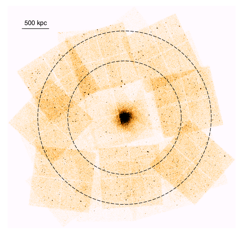
Figure 1.— Merged 2-8 keV band image of the Abell 133 region. The image is smoothed with a Gaussian kernel of five pixel radius. $R_{500}$ (1044 kpc or 15.4′) and $R_{200}$ (1596 kpc or 26.6′) are denoted as the inner and outer black dashed lines, respectively.

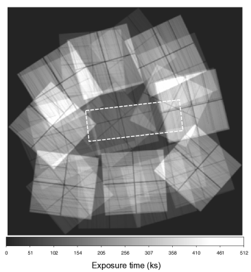
Figure 2.— Exposure map with respect to the merged 2-8 keV band image. The white dotted rectangle indicates ACIS-S data (Obs ID: 2203)

Figure 3.— Survey area as a function of effective exposure time in 2-8 keV band. A total of 72% of the total survey area (0.55/0.76 deg²) has exposures $>$150 ks (see vertical dotted line).

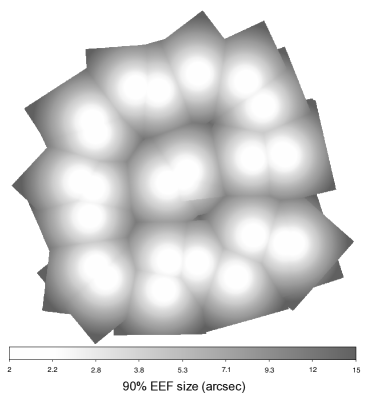
Figure 4.— Enclosed energy fraction map at 4.510 keV with respect to the merged 2-8 keV image.

Table 1Chandra Observing Log for Abell 133

Obs ID	Obs. Start	Exp	RA	DEC	Obs Cycle	Ref.
(1)	(2)	(3)	(4)	(5)	(6)	(7)
		(ks)	(deg)	(deg)
2203	2000 Oct 13	$35.46$	$15.672$	$-21.878$	$2$	1
3183	2002 Jun 24	$44.52$	$15.670$	$-21.878$	$3$	2
3710	2002 Jun 26	$44.59$	$15.670$	$-21.878$	$3$	2
9897	2008 Aug 29	$69.22$	$15.674$	$-21.881$	$9$	3
12177	2010 Aug 31	$50.11$	$15.453$	$-22.062$	$11$	4
12178	2010 Sep 7	$46.83$	$15.999$	$-22.002$	$11$	4
12179	2010 Sep 3	$51.10$	$15.735$	$-22.141$	$11$	4
13391	2011 Aug 16	$46.43$	$15.757$	$-22.233$	$12$	4
13392	2011 Sep 16	$49.89$	$15.639$	$-21.563$	$12$	4
13442	2011 Aug 23	$176.69$	$15.350$	$-21.818$	$12$	4
13443	2011 Aug 26	$69.68$	$15.359$	$-21.812$	$12$	4
13444	2011 Sep 3	$38.26$	$15.774$	$-21.613$	$12$	4
13445	2011 Sep 2	$65.18$	$15.514$	$-22.193$	$12$	4
14333	2011 Aug 31	$134.76$	$15.774$	$-21.613$	$12$	4
13446	2011 Sep 9	$58.42$	$15.480$	$-21.587$	$12$	4
13447	2011 Sep 8	$69.13$	$15.983$	$-21.744$	$12$	4
14338	2011 Sep 10	$117.50$	$15.480$	$-21.587$	$12$	4
13448	2011 Sep 13	$146.12$	$15.993$	$-21.710$	$12$	4
13449	2011 Sep 6	$68.15$	$15.424$	$-21.662$	$12$	4
14343	2011 Sep 12	$35.30$	$15.993$	$-21.710$	$12$	4
13451	2011 Sep 16	$70.12$	$15.947$	$-22.196$	$12$	4
13452	2011 Sep 24	$142.07$	$15.322$	$-22.089$	$12$	4
14345	2011 Sep 23	$33.74$	$15.322$	$-22.089$	$12$	4
13454	2011 Sep 19	$91.79$	$16.030$	$-21.897$	$12$	4
14346	2011 Sep 21	$85.90$	$16.030$	$-21.897$	$12$	4
13456	2011 Oct 15	$135.63$	$15.635$	$-22.148$	$12$	4
14354	2011 Oct 10	$38.64$	$15.635$	$-22.148$	$12$	4
13518	2011 Sep 17	$49.60$	$15.739$	$-21.901$	$12$	4
13450	2011 Oct 5	$108.18$	$15.975$	$-22.161$	$12$	4
14347	2011 Oct 9	$68.69$	$15.975$	$-22.161$	$12$	4
13453	2011 Oct 13	$68.95$	$15.841$	$-21.604$	$12$	4
13455	2011 Oct 19	$69.63$	$15.983$	$-21.916$	$12$	4
13457	2011 Oct 21	$69.13$	$15.341$	$-22.086$	$12$	4

Note. — The ‘RA’ and ‘Dec’ columns indicate the pointing centers of each Chandra observation.

References. — Reference where data were first published: (1) Fujita et al. (2002); (2) Vikhlinin et al. (2005); (3) Sun (2009); (4) Morandi & Cui (2014).

III. Analysis

III.1. Point source detection

To detect X-ray point sources in our mosaic image, we first constructed an ‘EEF map’, where each pixel represents the 90% EEF at 1.5 keV (for soft band) and 4.5 keV (for hard band, see Figure 4). The EEF map for the full band is made by averaging our soft- and hard-band maps. The final EEF was taken as the minimum EEF value of all exposures that contributed to each pixel in the mosaic, under the assumption that the exposure with the smallest EEF contributed the most weight. Next, we searched for point sources using wavdetect (Freeman et al., 2002), adopting wavelet scales of 1, 1.4, 2, 2.8, 4, 5.7, 8, 11.3, and 16, and a threshold significance of $10^{-5}$ (we adopted a relatively high threshold to avoid rejecting real sources at this point in the analysis, at the cost of increased contamination from spurious sources; see, e.g., Alexander et al. 2001). In this process we initially detected 1639 (full band), 1069 (full band), and 1461 (soft band) X-ray point sources.

To remove false positives from this initial list of X-ray sources, we followed Lehmer et al. (2012) and Ehlert et al. (2013) and calculated the probability that a detected source was spurious via the no-source binomial probability:

$$P=\sum\limits_{x\geq S}^{N}\frac{N!}{x!(N-x)!}p^{x}(1-p)^{n-x},$$ (1)

where $N$ is the total number of source and background counts within a source aperture, $S$ is the number of source counts in that aperture, and $p=1/(1+\rm\Omega_{bkg}/\Omega_{src}$), where $\rm\Omega_{src}$ and $\rm\Omega_{bkg}$ are the areas of source and background apertures, respectively. For example, we identified 38, 50, and 87 sources in the hard band as spurious when we used $P>0.007,0.004,$ and $0.001$, respectively. In the previous work by Luo et al. (e.g., 2017), the value of the no-source binomial probability was empirically determined to balance high reliability (minimizing the number of spurious targets) and high completeness (large number of targets) based on multiwavelength information. Since we do not have multiwavelength constraints on the potential X-ray sources, we adopted $P>0.007$ to remove false positives by following Luo et al. (2017) and the final catalog contains 1617 (full band), 1028(hard band), and 1324 (soft band) X-ray point sources.

III.2. Astrometry correction

To improve the accuracy of the positions of the detected X-ray point sources, we applied an astrometry correction by searching for optical counterparts, using archival images from the Canada-France-Hawaii telescope (CFHT). Eleven g-band images were taken as a mosaic to cover 1 square degree with the total exposure time of 1320s and 5$\sigma$ limiting magnitude is 26.5. We cross-matched the 1028 X-ray point sources detected in hard band with the list of 694 optical point sources with $g$-band magnitudes brighter than 19 mag, using the CIAO tool wcs_match with a 3″ matching radius and 0$\farcs$6 residual limit. We identified 30 optical counterparts, with which we used the tool wcs_update to update the X-ray astrometry, which included shifts in the x (east-west) and y (south-north) directions by -1.1 and -0.1 pixels, respectively, and in rotation by 0.01$\arcdeg$ (counter-clockwise). We note that we tried to correct the astrometry for individual exposures (prior to merging) similarly to several prior works for deep fields (e.g., Luo et al., 2017). However, we found that the astrometry correction for individual exposure introduced additional uncertainties for our dataset mainly due to the lower exposure time of each exposure. Thus, we decided to correct the astrometry after merging. We do not discuss optical properties in this paper. However, for reference, we tabulate available information on matched optical counterparts in our final X-ray catalog (see Section 3.4).

III.3. Flux estimation

To measure the X-ray flux of each point source, we adopted a source aperture as the radius set to the value of the 90% EEF at the position of each source. The number of background counts per pixel was estimated using a background image for which we excised all detected sources identified by wavdetect (i.e., including spurious sources), using the annuli with inner and outer radii between 2 and 3 times the 90% EEF. We then calculated the net number of counts in each source aperture, to which we applied a 90% aperture correction. Corresponding error is estimated at the 90% confidence level, assuming Poisson statistics (Gehrels, 1986).

We converted the net count rates to fluxes using conversion factors calculated from WEBPIMMS. For the conversion factor, we adopted the Chandra Cycle 12 effective area curves (the vast majority of our observations were taken in cycle 12), and a power-law model with photon index $\Gamma=1.4$ (i.e., $N_{E}\propto E^{-1.4}$, where $N_{E}$ is the photon flux density and $E$ is the photon energy) and foreground Galactic absorption with a column density $N_{\rm H}=1.6\times 10^{20}\,{\rm cm^{-2}}$. Our adopted column density was determined as the average value from the Dickey & Lockman (1990) H I maps, which range from 1.4-1.6$\times 10^{20}\rm\ cm^{-2}$ across the field of view of our Chandra mosaic. We note that the effects from our choices for Cycle number and column density are not significant, only introducing $\lesssim$ 5% and 1% systematic errors from Cycle number and column density, respectively. To estimate unabsorbed fluxes at each band, we obtained a conversion factor of $1.233\times 10^{-11}$ , $6.109\times 10^{-12}$ and $2.214\times 10^{-11}\,\rm erg/s$/cm² per 1 count/s, for the full-, soft- and hard- bands respectively.

Since we have no information on the distance to individual X-ray sources, we are not able to calculate X-ray luminosities for each source, nor can we ascertain on an individual basis if the X-ray sources are associated with the cluster (or if they are foreground/background sources). In the hard band, the minimum flux among the detected targets is $4.3\times 10^{-16}\,\rm erg\ s^{-1}cm^{-2}$, which would correspond to a luminosity of 7.9 $\times 10^{38}\,\rm erg\ s^{-1}$ at the distance of Abell 133. At such low luminosities, there could be contaminations from low mass X-ray binaries and high mass X-ray binaries within the 90% Chandra EEF (if at the cluster redshift; e.g., Grimm et al., 2003; Gilfanov, 2004; Mineo et al., 2012; Lehmer et al., 2014). However, due to the lack of the distance information, we make no attempt to estimate X-ray binary contribution fractions, as such an investigation would require further multi-wavelength data (e.g., optical spectra to determine redshifts of optical counterparts).

Table 2Main Chandra source catalog

	X-ray coordinates						Optical coordinates
#	RA	DEC	FB	SB	HB	HR	RA	Dec	$g$ mag	$g-r$	$\alpha_{ox}$
(1)	(2)	(3)	(4)	(5)	(6)	(7)	(8)	(9)	(10)	(11)	(12)
1	15.17015	-22.05955	$1751.5_{-68.3}^{+70.4}$	$1217.0_{-56.8}^{+59.0}$	$490.3_{-35.8}^{+38.0}$	$-0.43_{-0.04}^{+0.04}$	15.17018	-22.05977	19.30	0.04	1.43
2	15.18871	-22.06865	$119.2_{-17.4}^{+19.6}$	$69.8_{-13.2}^{+15.4}$	$25.4_{-7.7}^{+10.0}$	$-0.47_{-0.18}^{+0.21}$	—	—	—	—	—
3	15.19384	-22.04413	$99.1_{-15.8}^{+18.0}$	$26.8_{-7.9}^{+10.2}$	$46.9_{-10.7}^{+12.9}$	$0.27_{-0.19}^{+0.23}$	—	—	—	—	—
4	15.19691	-21.89512	$349.3_{-30.2}^{+32.3}$	$173.0_{-21.0}^{+23.2}$	$105.0_{-16.3}^{+18.5}$	$-0.24_{-0.10}^{+0.11}$	—	—	—	—	—
5	15.20327	-22.02950	$61.6_{-12.3}^{+14.6}$	$9.6_{-4.5}^{+6.9}$	$29.7_{-8.4}^{+10.6}$	$0.51_{-0.27}^{+0.36}$	—	—	—	—	—
Note – Col. (2-3): Right ascension and Declination of X-ray point source. Col. (4-6): Net counts in full- (0.5-8 keV), soft- (0.5-2 keV), and hard-(2-8 keV)
band. The conversion factors from the net counts to the fluxes are $1.233\times 10^{-11}$, $6.109\times 10^{-12}$, and $2.214\times 10^{-11}\,\rm erg/s$/cm2 per 1 count/s for the full-, soft-
and hard- bands respectively. Col. (7): Hardness ratio. Col. (8-9): Right ascension and Declination of optical counterpart. Col. (10): $g$-magnitude. Col. (11):
$g-r$ color. Col. (12): optical to X-ray power-law slope. Table 2 is published in its entirety in the machine-readable format. A portion is shown here for guidance
regarding its form and content.

III.4. Main Chandra source catalog

Using the detected sources in three bands, we construct a main Chandra source catalog. We cross-matched the detected point sources in the three bands using matching radii of 2.5″ for point sources located within 6′ from the closest aimpoint (see e.g., Figure 4) and 4″ for the others. The main Chandra source catalog includes 1952 point sources, which are detected in at least one of the three bands (Table 2). We estimated net counts for each band with the uncertainty of 90% confidence level, and upper limits are at 95% confidence (2$\sigma$). For sources detected in both soft- and hard-bands, we calculated hardness ratios:

$${\rm Hardness\ ratio}=\frac{H-S}{H+S},$$ (2)

where $H$ and $S$ are the number counts in hard band and soft bands, respectively. In Table 2, RA and Dec information is adopted from the order of hard-, full-, and soft- bands.

We also provide optical information for any X-ray point source that has an optical counterpart. To identify optical counterparts, we consider 15093 optical points sources with $r_{\rm mag}<22.5$ in our CFHT images Out of 1951 X-ray detections, we found optical counterparts for 310 sources adopting a matching radius of 1.5″ which is adopted in e.g., Xue et al. (2011); Luo et al. (2017). In Table 2, we present their optical positions, the $g$ magnitude, $g-r$ color, and optical to X-ray spectral index $\alpha_{\rm ox}$=-0.384 ${\rm log}\ (f_{2\rm kev}/f_{2500{\rm\textup{\AA}}})$ (Tananbaum et al., 1979). We note that $f_{2\rm kev}$ was converted from full band flux, assuming a photon index $\Gamma=1.4$ and $f_{2500{\rm\textup{\AA}}}$ was estimated by extrapolating from $g$ magnitude, assuming $\alpha_{\rm\lambda}=-1.56$ (Vanden Berk et al., 2001).

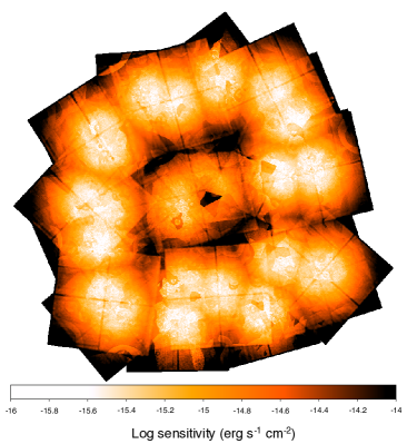
Figure 5.— The sensitivity map with respect to the merged 2-8 keV image.

III.5. Sensitivity map

To understand the completeness of our survey we constructed a sensitivity map for each band, following an algorithm outlined by Ehlert et al. (2013). Our sensitivity map provides the minimum number of photons required for a detection at every pixel position, with respect to the background. We first made a background image by excising regions containing X-ray point sources (masking twice the 90% EEF size, using the CIAO tool roi), and we then randomly replaced pixel values within each excised region assuming Poisson noise, based on the distribution of counts in annuli with radii spanning 2-3$\times$ the 90% EEF (using the tool dmfilth).

To build the sensitivity map, we defined local and global backgrounds at the positions of every pixel. The local backgrounds were calculated from the background image described above, using annuli centered on each pixel with inner and outer radii of 2 and 3 times the 90% EEF, respectively. For the global backgrounds, we utilized the merged image (i.e., including the X-ray point sources), from which we adopted the maximum number of counts for any source that falls within an annulus spanning 10-20 times the 90% EEF. If there were no point source within that annulus, then we adopted as the global background the number of counts from the closest point source. By using this strategy, we can minimize the p value and the photon number counts required for a detection. In Equation 1, we then adopted $S$ as the number of the local background counts, $N$ as the total number of the local and global background counts, and $p=1/(1+\rm\Omega_{global}/\Omega_{local}$), where $\rm\Omega_{local}$ and $\rm\Omega_{global}$ are the areas of the local background and the global background, respectively. We then calculated the minimum number of counts ($x$) to yield $P<0.007$, which represents the minimum number of counts required for a detection at each pixel. From these count limits, the exposure map, and the previously determined conversion factors, we derived the flux sensitivity map and the map in the hard band is shown in Figure 5. Note that the sensitivity varies dramatically from $\sim 10^{-16}\ {\rm to}\ 10^{-13}\ \rm erg\ s^{-1}\ cm^{-2}$ across the survey field of view.

Figure 6 shows the cumulative survey area as a function of sensitivity, and we tabulate various completeness flux thresholds from 90% completeness down to 20% in Table 3. We also quote corresponding luminosities at the distance of Abell 133 in Table 3, and the number of detected X-ray point sources above each flux threshold. Through the rest of this paper, particularly in §4.2, we define high- and low-flux subsamples based on a threshold of the 80% completeness level.

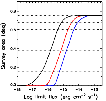
Figure 6.— Survey area as a function of the flux detection sensitivity limit. Horizontal dotted lines mark the flux limits for 100%, 90%, 80%, 50%, and 20% sky coverage (from top to bottom). Black, red, and blue indicate soft-, full-, and hard- bands, respectively.

Table 3Flux Limits and Completeness

Completeness (%)	$\rm f_{0.5-8}keV$	$\rm f_{0.5-2}keV$	$\rm f_{2-8}keV$
(1)	(2)	(3)	(4)
	erg $\rm cm^{-2}\ s^{-1}$	erg $\rm cm^{-2}\ s^{-1}$	erg $\rm cm^{-2}\ s^{-1}$
90	$3.38\times 10^{-15}$	$7.08\times 10^{-16}$	$8.50\times 10^{-15}$
80	$2.04\times 10^{-15}$	$4.26\times 10^{-16}$	$4.75\times 10^{-15}$
50	$6.95\times 10^{-16}$	$1.43\times 10^{-16}$	$1.57\times 10^{-15}$
20	$2.20\times 10^{-16}$	$3.83\times 10^{-17}$	$5.55\times 10^{-16}$

Note. — Col. (1): completeness level. Col. (2-4): flux limit for each band for given completeness.

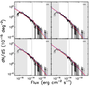
Figure 7.— Differential number count distribution in the hard band with various fitting ranges. Black circles denote data points included in the model fits, and grey circles in each grey shaded region are omitted. The red solid line indicates the best-fit to our broken power laws model. Error bars indicate 1sigma confidence levels. The blue dashed and purple dotted lines show the results for the ChaMP field (Kim et al., 2007) and the CDF-S field (Lehmer et al., 2012), respectively. The vertical dotted line denotes the break flux.

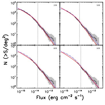
Figure 8.— Cumulative number count distribution in the hard band with various fitting ranges. Black- and grey solid shows the our result within and out of fitting range. The grey shaded area indicates the 1$\sigma$ confidence level. Other symbols have the same meaning as in Figure 7.

Table 4Model parameters for number distribution

Completeness (%)	$\rm fluxlimit$	$K$	$\gamma_{1}$	$\gamma_{2}$	$S_{b}$
	(erg $\rm cm^{-2}\ s^{-1}$)
(1)	(2)	(3)	(4)	(5)	(6)
Full band
Cumulative number count distribution
20	$2.20\times 10^{-16}$	$951\pm 41$	$1.32\pm 0.04$	$2.91\pm 0.14$	$18.9\pm 1.0$
50	$6.95\times 10^{-16}$	$1470\pm 19$	$1.51\pm 0.01$	$2.40\pm 0.03$	$13.2\pm 0.3$
80	$2.04\times 10^{-15}$	$1629\pm 21$	$1.54\pm 0.01$	$2.54\pm 0.02$	$14.4\pm 0.4$
90	$3.38\times 10^{-15}$	$1618\pm 28$	$1.55\pm 0.01$	$2.52\pm 0.02$	$14.6\pm 0.4$
Differential number count distribution
20	$2.20\times 10^{-16}$	$577\pm 53$	$0.99\pm 0.10$	$3.02\pm 0.41$	$11.9\pm 2.4$
50	$6.95\times 10^{-16}$	$753\pm 57$	$1.11\pm 0.05$	$2.75\pm 0.26$	$10.0\pm 1.8$
80	$2.04\times 10^{-15}$	$688\pm 68$	$1.08\pm 0.05$	$2.79\pm 0.28$	$10.3\pm 1.9$
90	$3.38\times 10^{-15}$	$689\pm 62$	$1.11\pm 0.06$	$2.70\pm 0.26$	$10.4\pm 1.9$
Soft band
Cumulative number count distribution
20	$3.83\times 10^{-17}$	$584\pm 7$	$0.96\pm 0.01$	$2.24\pm 0.02$	$1.9\pm 0.0$
50	$1.43\times 10^{-16}$	$585\pm 5$	$1.20\pm 0.02$	$2.12\pm 0.01$	$1.8\pm 0.0$
80	$4.26\times 10^{-16}$	$632\pm 10$	$1.36\pm 0.05$	$2.07\pm 0.02$	$1.6\pm 0.0$
90	$7.08\times 10^{-16}$	$659\pm 12$	$1.37\pm 0.04$	$2.08\pm 0.02$	$1.6\pm 0.0$
Differential number count distribution
20	$3.83\times 10^{-17}$	$729\pm 128$	$0.60\pm 0.14$	$1.89\pm 0.08$	$0.8\pm 0.1$
50	$1.43\times 10^{-16}$	$607\pm 44$	$1.09\pm 0.08$	$1.87\pm 0.07$	$0.9\pm 0.1$
80	$4.26\times 10^{-16}$	$637\pm 103$	$1.16\pm 0.24$	$1.88\pm 0.07$	$0.8\pm 0.1$
90	$7.08\times 10^{-16}$	$664\pm 89$	$1.40\pm 0.28$	$1.89\pm 0.06$	$0.7\pm 0.1$
Hard band
Cumulative number count distribution
20	$5.55\times 10^{-16}$	$1370\pm 20$	$1.67\pm 0.02$	$2.75\pm 0.07$	$16.3\pm 0.6$
50	$1.57\times 10^{-15}$	$1543\pm 41$	$1.67\pm 0.01$	$2.78\pm 0.05$	$13.2\pm 0.8$
80	$4.75\times 10^{-15}$	$1393\pm 47$	$1.71\pm 0.01$	$2.66\pm 0.03$	$15.7\pm 0.8$
90	$8.50\times 10^{-15}$	$1354\pm 50$	$1.76\pm 0.01$	$2.54\pm 0.03$	$16.1\pm 0.7$
Differential number count distribution
20	$5.55\times 10^{-16}$	$903\pm 159$	$1.44\pm 0.12$	$2.95\pm 0.64$	$13.1\pm 2.5$
50	$1.57\times 10^{-15}$	$1265\pm 79$	$1.60\pm 0.04$	$2.77\pm 0.34$	$11.0\pm 1.9$
80	$4.75\times 10^{-15}$	$1218\pm 118$	$1.64\pm 0.05$	$2.68\pm 0.36$	$11.7\pm 2.1$
90	$8.50\times 10^{-15}$	$1112\pm 713$	$1.63\pm 0.27$	$2.42\pm 0.50$	$13.1\pm 7.9$

Note. — Col. (1): completeness level. Col. (2): flux limit for given completeness. Col. (3): normalization factor. Col. (4): faint end slope. Col. (5): bright end slope. Col. (6): break flux in unit of $10^{-15}\rm erg\ s^{-1}cm^{-2}$.

IV. Results and discussion

IV.1. Number count distribution

For our detected X-ray point sources, we investigate cumulative and differential number counts. The cumulative number counts above the given flux, $S$, is

$$N(>S)=\sum\limits_{S_{i}\geq S}\frac{1}{\Omega_{i}},$$ (3)

where the $\Omega_{i}$ is the survey area at the given flux of the $i$th source.

The differential number counts is the derivative form of cumulative number counts, and can be calculated as follows:

$$\frac{dN}{dS}\bigg{\rvert}_{i}=-\frac{N_{i+1}-N_{i}}{S_{i+1}-S_{i}},$$ (4)

The distributions for X-ray point sources in previous works are represented by a double (or broken) power law (see e.g., Kim et al., 2007; Lehmer et al., 2012; Luo et al., 2017). We adopt the same equations here as Kim et al. (2007):

$$\frac{dN}{dS}=\begin{cases}-K(S/S_{ref})^{-\gamma_{1}},&\text{$S<S_{b}$}.\\ -K(S_{b}/S_{\rm ref})^{\gamma_{2}-\gamma_{1}}(S/S_{\rm ref})^{-\gamma_{2}},&\text{$S>S_{b}$}\end{cases}$$ (5)

$$N(>S)=\begin{cases}K\Big{(}\frac{1}{1-\gamma_{1}}-\frac{1}{1-\gamma_{2}}\Big{)}\Big{(}\frac{S_{b}}{S_{\rm ref}}\Big{)}^{(1-\gamma_{1})}\\ +K\Big{(}\frac{1}{\gamma_{1}-1}\Big{)}\Big{(}\frac{S}{S_{\rm ref}}\Big{)}^{1-\gamma_{1}},&\text{$S<S_{b}$}\\ -K\Big{(}\frac{1}{\gamma_{2}-1}\Big{)}\Big{(}\frac{S_{b}}{S_{\rm ref}}\Big{)}^{(\gamma{2}-\gamma_{1})}\Big{(}\frac{S}{S_{\rm ref}}\Big{)}^{1-\gamma_{2}},&\text{$S>S_{b}$}\end{cases}$$ (6)

where the $\gamma_{1}$ and $\gamma_{2}$, are the faint- and bright- end slopes, K is a normalization factor, and $S_{b}$ is a break flux. $S_{\rm ref}$ is a normalization flux. which we set to $10^{-15}\rm erg\ s^{-1}cm^{-2}$.

In our fitting, we adopt four flux ranges with different minimum fluxes, each corresponding to the 20%, 50%, 80%, and 90% completeness levels, which are presented in Table 3, in order to investigate the effect from sensitivity. The maximum flux density is the same for all four subsamples ($3.74\times 10^{-13}$, $1.49\times 10^{-13}$, $2.16\times 10^{-13}\rm\ erg\ s^{-1}\ cm^{-2}$ for full-, soft-, and hard- bands respectively). To estimate the uncertainties of the model parameters, we conducted Monte Carlo simulations with 1000 mock distributions generated by using errors calculated following Gehrels (1986). We then refit the model to each mock distribution. We take the median and the standard deviation of the N=1000 distributions for each parameter as the best-fit value and the error bar. We note that we fit the differential and cumulative number count distributions separately, which yielded different model parameters. This might be due to the small number of detections in the differential number counts in the high flux regime, and hence uncertainties for the differential number counts are much larger than those for the cumulative number counts. We provide the model parameters for the differential and cumulative number count distributions for each completeness level in each band in Table 4.

As examples we present the differential and cumulative number count distribution in the hard band with the best-fit model (red solid) for the four various fitting ranges in Figures 7 and 8, respectively. The black symbols (in Figure 7) and lines (in Figure 8) denote the data included in each fit. In each panel, we also plot distributions from the Chandra Multiwavelength Project (ChaMP) fields (purple dotted lines; Kim et al., 2007) and the CDF-S fields (blue dashed lines; Lehmer et al., 2012) for comparison.

As shown in Table 4 and in Figure 7 and 8, we find that the best-fit model parameters vary depending on the flux range included in the fit. It seems that including lower fluxes in the fit causes $\gamma_{1}$ to be higher and $\gamma_{2}$ to be lower. The normalization factor and the break flux also vary, but they do not show significant dependences on the adopted minimum flux. As shown in Figure 7, the differential number counts below $\sim 10^{-15}\rm erg\ s^{-1}cm^{-2}$ are smaller as flux decreases, and this feature affects the fitting results by including or excluding such low number counts at the faint flux end. Similarly to the hard band, fitting results for distributions in full-, and soft- bands also show strong dependency on fitting range (Table 4). This result suggests that statistical uncertainties can be an issue in the low flux regime, hence the fitting range range should be carefully considered in the analysis of number count distributions.

Interestingly, there are large differences even between previous works except for $\gamma_{2}$ (consistent within uncertainties). For example, for the distribution in the hard band, $\gamma_{1}$ are 1.82$\pm$0.01 and 1.58$\pm$0.01 for ChaMP and ChaMP+CDF-S (Kim et al., 2007) and 1.32$\pm$0.04 for CDF-S (Lehmer et al., 2012) giving $\sim 0.5$ dex difference. This shows that the low flux regime is more sensitive to the adopted completeness level than the high flux regime and that one needs to consider the fitting range carefully.

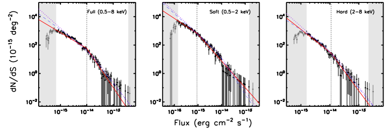
Figure 9.— Differential number count distribution in the full-, soft-, and hard- bands with best-fit model (red) fitted over the 50% sensitivity level. Symbols and colors are same with Figure 7.

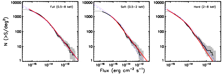
Figure 10.— Cumulative number count distribution in the full-, soft-, and hard- bands with best-fit model (red) fitted over the 50% sensitivity level. Symbols and colors are same with Figure 8.

IV.2. Normalization in number count distribution

In Figures 9 and 10, we plot the differential- and cumulative- number counts in the three bands with the best-fit model fitted over the 50% sensitivity level. Interestingly, our results, at least in the soft- and hard- bands, show somewhat lower normalizations to the cumulative number count distribution compared to the distributions of X-ray point sources in the fields (Kim et al., 2007; Gilmour et al., 2009; Lehmer et al., 2012; Ehlert et al., 2013). For example, from 50% completeness level to $10^{-13}\ {\rm erg\,s^{-1}\,cm^{-2}}$, our distribution in soft- and hard- bands are on average $\sim 22$% lower than the that of the ChaMP. Below, we discuss possible reasons for this discrepancy, including 1) environmental effects, 2) cosmic variance, and 3) systematic errors.

First, the large-scale cluster environment can potentially affect the number of detected X-ray point sources (e.g., Gilmour et al., 2009; Ehlert et al., 2013). However, we do not expect environmental effects to be significantly altering the $\log N-\log S$ distribution across the Abell 133 field. For example, if AGN activities are suppressed in a cluster environment, then the $\log N-\log S$ distribution should be similar compared to that in a non-cluster environment, since the number of foreground/background cosmic X-ray sources will be similar regardless of environmental effects. On the other hand, if AGN activities are enhanced within cluster environments (e.g., Gilmour et al., 2009; Ehlert et al., 2013), then the $\log N-\log S$ distribution should have a higher normalization. Thus, it is difficult to understand how the enhanced AGN activities in a cluster environment can yield the lower $\log N-\log S$ normalization that we observe in the Abell 133 field.

Second, we consider the possibility of a different normalization due to cosmic variance. Luo et al. (2008) reported that the normalization of the $\log N-\log S$ distribution from the CDF-S is $\sim$ 25% smaller than that from the CDF-N, suggesting a possibility that the difference may be caused by field to field variations. Wide-field surveys of more regions of the sky are required to quantify the level to which the normalization of $\log N-\log S$ might vary from field to field.

Finally, there could be systematic uncertainties introduced from different (or inconsistent) analyses (i.e., including lower fluxes in the fitting) among various works. To find out the systematic differences among various studies is beyond the scope of this study.

IV.3. Radial distribution of number densities

The inner $\approx$3$\arcmin$ of the Abell 133 cluster contains diffuse X-ray emission from hot gas (see Figure 1), which could degrade the sensitivity for detecting point sources in the inner region compared to the cluster outskirts. Below, we investigate if the presence of diffuse emission can affect our $\log N-\log S$ distribution, particularly for the low-flux sources.

We separate the X-ray point sources into two groups, which are divided by the flux sensitivity limit at the 80% completeness. We then compare the source count distributions in the three bands as a function of the distance from the center of the cluster, which is determined as the location of peak diffuse X-ray emission as RA: 15.6737$\arcdeg$, DEC: -21.8815$\arcdeg$ (see Figure 11).

The subset of the high-flux objects shows a relatively flat distribution with the radius, which is expected if the majority of the point sources are foreground/background objects. In contrast, we find a small peak at the innermost region ($<$0.25 Mpc, or 3.8 ′), while the region beyond $R_{200}$ (i.e., $\gtrsim$1.6 Mpc or 24.2 ′) shows a decline in the source counts, plausibly due to the poor sensitivity at large radial distance (see Figure 5). We note that the sensitivity inside of $R_{200}$ is mostly higher than the 80% completeness, meaning that the high flux sample is not highly incomplete within $R_{200}$ because of low-sensitivity. The peak in the central region suggests that we are not missing high-flux sources embedded in the diffuse emission. If we assume that the contamination of the non-cluster member X-ray point sources is constant along the radius, the central peak in the radial distribution is consistent with the results reported in the previous studies (e.g., Gilmour et al., 2009; Ehlert et al., 2013). Since the galaxy number density is steeply decreasing as a function of radius, the weak increase of the X-ray point source at the center is still consistent with the radial decrease of AGN fraction. For example, the galaxy number density typically decreases by $\sim$an order of magnitude from R₅₀₀ to the center (e.g., Popesso et al., 2007), while the number density of the X-ray point source decreases by only a factor of a few in Abell 133. In Figure 12, we present the AGN fraction for the high flux subsamples, which is calculated as (e.g., Ehlert et al., 2013)

$$\phi=\frac{N_{X}(r)-C_{x}}{N_{G}(r)},$$ (7)

where $N_{X}(r)$ and ${N_{G}(r)}$ are the number densities of X-ray point sources and galaxies. The galaxy number density was estimated assuming a King model with a core radius of $r_{c}/r_{200}$=0.224 (see Popesso et al. 2007). $C_{x}$ is the number density of the background, and we adopted the values of 646, 556, and 302 for full-, soft-, and hard- bands, respectively, which are the average of the number densities at 2 Mpc and 2.25 Mpc. The observed radial trend in Abell 133 would imply that AGN fraction decreases toward the cluster center, suggesting the lower level of AGN triggering in denser environments (e.g., Gilmour et al., 2009; Ehlert et al., 2013). We note that the AGN fraction calculated here is sensitive to the background, which was arbitrarily selected. The reason for the arbitrary selection is that we do not know the actual number density of the background. Thus, at ¡1.6 Mpc, the uncertain background subtraction may lead to the positive slope shown in Figure 12. For a more reliable estimation, individual cluster members should be identified, which is beyond the scope of this paper. We also note that the decrease in AGN fraction at ¿1.6 Mpc is likely caused by poor sensitivity.

On the other hand, the trend for the low-flux objects is different. For example, we detect the lower number of the low-flux sources in the innermost region ($<$0.25 Mpc), which is likely caused by the low-flux sources being diluted below the detection threshold by the diffuse X-ray emission. Interestingly, we find an excess of low-flux sources at moderate radii, i.e., at 1.0–1.5 Mpc. This trend could be due to a sensitivity effect. As seen in Figure 5, the sensitivity at 1.0–1.5 Mpc is higher than other regions, hence we may detect more low-flux sources. To understand this, we took average sensitivities in the hard band at 0.5–1.0 Mpc ($10^{-14.5}\,\rm erg\ s^{-1}cm^{-2}$) and 1.0–1.5 Mpc ($10^{-15.1}\,\rm erg\ s^{-1}cm^{-2}$) and compared the expected number densities based in each radial bin (using our cumulative number count distribution). The number densities are 1133 (at 0.5–1.0 Mpc) and 1956 (at 1.0–1.5 Mpc), consistent with our results (Figure 8). In addition to sensivity, gas clumpiness could be another factor influencing this trend. By investigating gas clumpiness in Abell 133 out to $R_{200}$, for example, Morandi & Cui (2014) reported that the gas clumping factor at radii beyond 1 Mpc (which corresponds to $R_{500}$) is larger than unity (i.e., a factor of 2-3). They interpreted that this result indicates that the hot gas is virialized interior to $R_{500}$, but not at larger radii. While one effect of diffuse emission would be to lower the sensitivity for detecting point sources, it is plausible that the clumpy gas at the moderate radius is instead introducing an excess of spurious low-flux X-ray sources, where gas clumps are improperly identified as points sources. We stress that effects from diffuse gas emission are not of concern for our high-flux subset. In other words, the diffuse emission does not affect the normalization of our $\log N-\log S$ distribution.

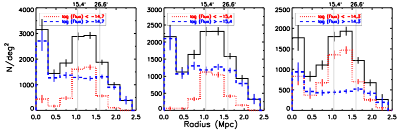
Figure 11.— The number density of sources in the full- (left), soft- (center), and hard- (right) bands as a function of distance from the cluster center. Black, red, and blue lines represent the full sample, the low flux subsample ($\log f_{\rm 0.5-8keV}<-14.7$, $\log f_{\rm 0.5-2keV}<-15.4$, and $\log f_{\rm 2-8keV}<-14.3$), the and high flux subsample ($\log f_{\rm 0.5-8keV}>-14.7$, $\log f_{\rm 0.5-2keV}>-15.4$, and $\log f_{\rm 2-8keV}>-14.3$), respectively. $R_{500}$ (left) and $R_{200}$ (right) are denoted as vertical gray lines. The uncertainties from Poisson statistic are shown at each radius bin.

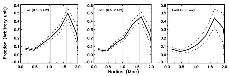
Figure 12.— X-ray point source fraction as a function of distance from the cluster center for high flux subsample ($\log f_{\rm 0.5-8keV}>-14.7$, $\log f_{\rm 0.5-2keV}>-15.4$, and $\log f_{\rm 2-8keV}>-14.3$). The dashed line shows the uncertainties from Poisson statistic. $R_{500}$ (left) and $R_{200}$ (right) are denoted as vertical gray lines.

V. Summary

We investigate X-ray point sources in a wide-field Chandra image (0.76 deg²) covering the Abell 133 cluster of galaxies at $z=0.0566$. From the relative deep X-ray mosaic images with a total exposure time of 2.8 Msec, we detect 1617, 1324, and 1028 X-ray point sources in the full-, soft-, and hard- bands with the flux limits at the 50% completeness level of $6.95\times 10^{-16},1.43\times 10^{-16},\rm\ and\ 1.57\times 10^{-15}$ erg s^-1 $\rm cm^{-2}$.. We present the X-ray point source catalog, which can be utilized for future multiwavelength studies of Abell 133 and its environment. The combined number counts of the X-ray point sources across the entire field are well represented with a broken power-law and the fitting parameters are in agreement with those of X-ray point source distributions in other fields. Similar to previous works (e.g., Gilmour et al., 2009; Ehlert et al., 2013), we find a slight excess of X-ray point sources that could be associated with the cluster, suggesting that AGN fraction decreases toward the cluster center, for given an increase of galaxy number density at the center. This result is consistent with the suppressed AGN activities in dense environments.

References

- Alexander et al. (2001) Alexander, D. M., Brandt, W. N., Hornschemeier, A. E., et al. 2001, AJ, 122, 2156
- Alexander et al. (2003) Alexander, D. M., Bauer, F. E., Brandt, W. N., et al. 2003, AJ, 126, 539
- Arnold et al. (2009) Arnold, T. J., Martini, P., Mulchaey, J. S., Berti, A., & Jeltema, T. E. 2009, ApJ, 707, 1691
- Boselli & Gavazzi (2006) Boselli, A., & Gavazzi, G. 2006, PASP, 118, 517
- Dickey & Lockman (1990) Dickey, J. M., & Lockman, F. J. 1990, ARA&A, 28, 215
- Ehlert et al. (2013) Ehlert, S., Allen, S. W., Brandt, W. N., et al. 2013, MNRAS, 428, 3509
- Elvis et al. (2009) Elvis, M., Civano, F., Vignali, C., et al. 2009, ApJS, 184, 158
- Fabian (2012) Fabian, A. C. 2012, ARA&A, 50, 455
- Freeman et al. (2002) Freeman, P. E., Kashyap, V., Rosner, R., & Lamb, D. Q. 2002, ApJS, 138, 185
- Fruscione et al. (2006) Fruscione, A., McDowell, J. C., Allen, G. E., et al. 2006, in Proc. SPIE, Vol. 6270, Society of Photo-Optical Instrumentation Engineers (SPIE) Conference Series, 62701V
- Fujita et al. (2002) Fujita, Y., Sarazin, C. L., Kempner, J. C., et al. 2002, ApJ, 575, 764
- Garmire et al. (2003) Garmire, G. P., Bautz, M. W., Ford, P. G., Nousek, J. A., & Ricker, Jr., G. R. 2003, in Proc. SPIE, Vol. 4851, X-Ray and Gamma-Ray Telescopes and Instruments for Astronomy., ed. J. E. Truemper & H. D. Tananbaum, 28–44
- Gehrels (1986) Gehrels, N. 1986, ApJ, 303, 336
- Gilfanov (2004) Gilfanov, M. 2004, MNRAS, 349, 146
- Gilli et al. (2007) Gilli, R., Comastri, A., & Hasinger, G. 2007, A&A, 463, 79
- Gilmour et al. (2009) Gilmour, R., Best, P., & Almaini, O. 2009, MNRAS, 392, 1509
- Grimm et al. (2003) Grimm, H.-J., Gilfanov, M., & Sunyaev, R. 2003, MNRAS, 339, 793
- Haggard et al. (2010) Haggard, D., Green, P. J., Anderson, S. F., et al. 2010, ApJ, 723, 1447
- Kim et al. (2007) Kim, M., Wilkes, B. J., Kim, D.-W., et al. 2007, ApJ, 659, 29
- Kormendy & Ho (2013) Kormendy, J., & Ho, L. C. 2013, ARA&A, 51, 511
- Lehmer et al. (2012) Lehmer, B. D., Xue, Y. Q., Brandt, W. N., et al. 2012, ApJ, 752, 46
- Lehmer et al. (2014) Lehmer, B. D., Berkeley, M., Zezas, A., et al. 2014, ApJ, 789, 52
- Luo et al. (2008) Luo, B., Bauer, F. E., Brandt, W. N., et al. 2008, ApJS, 179, 19
- Luo et al. (2017) Luo, B., Brandt, W. N., Xue, Y. Q., et al. 2017, ApJS, 228, 2
- Martini et al. (2013) Martini, P., Miller, E. D., Brodwin, M., et al. 2013, ApJ, 768, 1
- Mineo et al. (2012) Mineo, S., Gilfanov, M., & Sunyaev, R. 2012, MNRAS, 419, 2095
- Moran et al. (2005) Moran, S. M., Ellis, R. S., Treu, T., et al. 2005, ApJ, 634, 977
- Morandi & Cui (2014) Morandi, A., & Cui, W. 2014, MNRAS, 437, 1909
- Oh et al. (2014) Oh, S., Mulchaey, J. S., Woo, J.-H., et al. 2014, ApJ, 790, 43
- Popesso et al. (2007) Popesso, P., Biviano, A., Böhringer, H., & Romaniello, M. 2007, A&A, 464, 451
- Sun (2009) Sun, M. 2009, ApJ, 704, 1586
- Tananbaum et al. (1979) Tananbaum, H., Avni, Y., Branduardi, G., et al. 1979, ApJ, 234, L9
- Treu et al. (2003) Treu, T., Ellis, R. S., Kneib, J.-P., et al. 2003, ApJ, 591, 53
- Vanden Berk et al. (2001) Vanden Berk, D. E., Richards, G. T., Bauer, A., et al. 2001, AJ, 122, 549
- Vikhlinin et al. (2005) Vikhlinin, A., Markevitch, M., Murray, S. S., et al. 2005, ApJ, 628, 655
- Xue et al. (2011) Xue, Y. Q., Luo, B., Brandt, W. N., et al. 2011, ApJS, 195, 10