Baryonic susceptibilities, quark-diquark models, and quark-hadron duality at finite temperature

Abstract

Fluctuations of conserved charges such as baryon number, electric charge and strangeness may provide a test for completeness of states in lattice QCD for three light flavors. We elaborate on the idea that the corresponding susceptibilities can be saturated with excited baryonic states with an underlying quark-diquark structure with a linearly confining interaction. Using Polyakov-loop correlators we show that in the static limit, the quark-diquark potential coincides with the quark-antiquark potential in marked agreement with recent lattice studies. We thus study in a quark-diquark model the baryonic fluctuations of electric charge, baryon number and strangeness: $\chi_{BQ}$, $\chi_{BB}$ and $\chi_{BS}$; by considering a realization of the hadron resonance gas model in the light flavor sector of QCD. These results have been obtained by using the baryon spectrum computed within a relativistic quark-diquark model, leading to an overall good agreement with the spectrum obtained with other quark models and with lattice data for the fluctuations.

I Introduction

Quantum chromodynamics (QCD) is the fundamental non-Abelian gauge theory of strong interactions in terms of $2N_{c}N_{f}$ quarks and antiquarks and $2(N_{c}^{2}-1)$ gluons with $N_{c}=3$ the number of colors and $N_{f}=6$ the number of flavour species $u,d,s,c,b,t$. Quark and gluon confinement requires all physical states to be color singlet, but are the hadronic states a complete set of eigenstates of QCD spanning the Hilbert space ${\cal H}_{\rm QCD}$? This question is related to the validity and meaning of quark-hadron duality.

In the case of $N_{f}=3$ flavors, which will be assumed throughout the paper, the stable and low-lying bound states, such as the baryon octet and the pseudoscalar nonet are unambiguously part of the discrete spectrum. The remaining states belong to the continuum spectrum and are experimentally spotted in strong hadronic reactions, interpreted as unstable resonances and characterized by a mass and a width. They have been reported over the years by the Particle Data Group (PDG) booklet Patrignani et al. (2016) as single states rated with *,**,***,**** (for baryons) depending on the increasing confidence on their existence. However, are the PDG states complete and if so in what sense would they be complete?

For such resonance states, the verification of completeness for QCD in the continuum is subtle since within a Hamiltonian perspective they are not proper (normalizable) eigenstates of the QCD Hamiltonian, and besides, they correspond to unconventional representations of the Poincaré group Bohm and Sato (2005). Lattice QCD presents the clear advantage that in a finite box all states are discretized and hence become countable; below a certain maximal mass the number of states is finite as long as the volume $V$ remains finite (typically $V\sim(2-3\,\mathrm{fm})^{3}$). Resonances are extracted from those particular energy levels which become insensitive to the box size. The extent to which these states play a key role in the completeness issue is uncertain since, although there is a larger concentration of states around the resonance, in the bulk, the mass separation is $\Delta M\sim V^{-1/3}$.

In recent years, the thermodynamic approach to strong interactions pioneered by Hagedorn Hagedorn (1965, 1985) where the vacuum is represented by a non-interacting Hadron Resonance Gas (HRG), has emerged as a practical and viable path to establish completeness of hadronic states on a quantitative level in the hadronic phase. With all the provisos regarding the nature of resonance and bound states, the most impressive and vivid verification has been the recent study of the trace anomaly, $(\epsilon-3P)/T^{4}$ with $\epsilon$ energy density and $P$ the pressure. It was computed directly in lattice QCD by the Wuppertal-Budapest (WB) and the HotQCD collaborations Borsanyi et al. (2014); Bazavov et al. (2014) and the HRG model using the most recent compilation of the PDG states taking just their masses, i.e. assuming zero widths Patrignani et al. (2016) and for temperatures below $T\sim 170\,{\mathrm{MeV}}$. Remarkably, a similar degree of success is achieved within uncertainties Ruiz Arriola et al. (2014) (see Figs. 1 and 2) using the hadronic spectrum obtained in the Relativized Quark Model (RQM) of Capstick, Godfrey and Isgur Godfrey and Isgur (1985); Capstick and Isgur (1986) which predated the lattice QCD calculations by about 30 years. Finite width effects on the PDG (PDG-$\Gamma$) naturally provide a shift towards lower masses Ruiz Arriola et al. (2012); Broniowski (2016) as a consequence of the mass spectrum spread weighted by the exponentially decreasing Boltzmann factor.

This remarkable agreement becomes significantly spoiled when susceptibilities involving conserved charges such as the baryon number, the electric charge and the strangeness are considered Borsanyi et al. (2012); Bazavov et al. (2012). In particular, the differences between PDG, PDG-$\Gamma$ and the RQM become more visible and an excess of baryonic states as compared to the lattice QCD results is observed Ruiz Arriola et al. (2016) illustrating the so-called missing resonance problem.

In fact, since the early days of the quark model the extreme abundance of predicted and experimentally missing baryonic resonances has been a major cause of concern both at the theoretical as well as at the experimental level Capstick (1992) (see also Hey and Kelly (1983) and Capstick and Roberts (2000) for reviews and references therein). Possible ways out of the difficulties have traditionally been attributed either to a weak coupling of the predicted states to the particular production process (photo-production, $\pi N$ scattering etc.) or to a dynamical reduction of degrees of freedom due to diquark clustering.

The suspicion that the baryonic spectrum can be understood in terms of quark-diquark degrees of freedom is rather old (see e.g. Ref. Anselmino et al. (1993) for a review, but also Ref. Klempt et al. (2017) for evidence against it). This includes diquark clustering studies Fleck et al. (1988), non-relativistic Santopinto (2005) and relativistic Ferretti et al. (2011); Gutierrez and De Sanctis (2014) analyses where scalar and axial-vector diquarks have a mass of about $600\,{\mathrm{MeV}}$ and $800\,{\mathrm{MeV}}$ respectively (the diquark mass difference seems quite model independent and about $200\,{\mathrm{MeV}}$). As expected, in diquark models many states predicted by the quark model do not appear Capstick and Isgur (1986). More specifically, while not strictly forbidden, the relativistic diquark model Ferretti et al. (2011); Gutierrez and De Sanctis (2014) does not predict any missing states below $2\,{\mathrm{GeV}}$, whereas Isgur and Capstick have predicted five unobserved states Capstick and Isgur (1986). Lattice QCD has also provided insights, as some evidence on diquarks correlations in the nucleon Alexandrou et al. (2006) and the dominance of the scalar diquark channel DeGrand et al. (2008) have been reported. Moreover, the diquark-approximation has been found to work well in Dyson-Schwinger and Faddeev equations studies Eichmann et al. (2016). The radial Regge behavior found in the relativistic quark-diquark picture from a numerical study of the spectrum of the relativistic two-body problem Ebert et al. (2011) has been confirmed from a direct PDG analysis when the widths of the resonances are implemented in the analysis Masjuan and Ruiz Arriola (2017); Ruiz Arriola et al. (2017).

While the missing resonance problem has attracted a lot of interest both experimentally as well as theoretically, much of the discussion is focused on the individual one-to-one mapping of resonance states which have a mass spectrum and which are produced with different backgrounds. In contrast, the thermodynamic approach offers the possibility to perform a more global analysis where many of the fine details will hopefully be washed out due to the presence of the heat bath. In the present paper we profit from the new perspective provided by lattice QCD at finite temperature, based on separation of quantum numbers with the study of susceptibilities of conserved charges, where a combination of degeneracy and level density is involved. We try to answer the question whether or not quark-diquark baryonic states saturate the baryonic susceptibilities below the deconfinement crossover as compared to the available lattice QCD calculations Borsanyi et al. (2012); Bazavov et al. (2012). Aspects of quark-hadron duality at finite temperature have been discussed in pedagogical way in Ref. Ruiz Arriola et al. (2014). Actually, in a recent work it has been discussed how quark-hadron duality in deep inelastic scattering for baryons suggests an asymptotic quark-diquark spectrum with a linearly rising potential for scaling to hold in the structure functions Masjuan and Ruiz Arriola (2017); Ruiz Arriola et al. (2017). Motivated by this we want to establish if a similar pattern holds also at finite temperature.

The paper is organized as follows. In Section II we review the relevant aspects of the HRG model from the point of view of the Equation of State and the trace anomaly as compared to lattice QCD. In Section III we analyze the implications for fluctuations of conserved charges at finite temperature in the vacuum. then analyze in Section IV the quark-diquark potential obtained as a correlation function involving Polyakov loops. This allows to define our model and compute the spectrum by diagonalization in Section V where the susceptibilities are analyzed in terms of the free parameters of the theory. Finally in Section VI we come to the conclusions. In the appendices we provide details on the semiclassical determination of the spectrum and also prove a theorem on the sign of susceptibilities which is verified by lattice calculations.

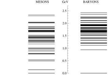
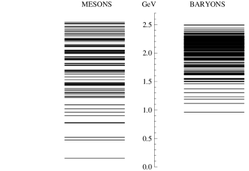
Figure 1: Left panel: Mesons and baryons spectrum made of $u$, $d$ and $s$ quarks from the PDG Tanabashi et al. (2018) (left panel), and from the Relativized Quark Model Godfrey and Isgur (1985); Capstick and Isgur (1986) (right panel).

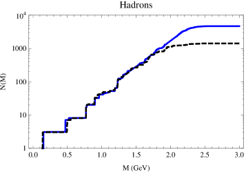
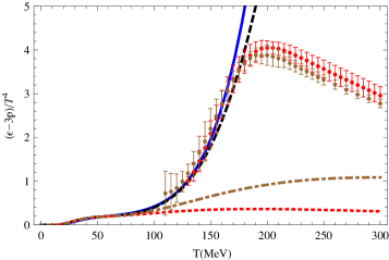
Figure 2: Left panel: Cumulative number for the PDG Tanabashi et al. (2018) (dashed line) and the RQM (solid) Godfrey and Isgur (1985); Capstick and Isgur (1986). Right panel: Trace anomaly as a function of temperature in lattice QCD Borsanyi et al. (2014); Bazavov et al. (2014) vs HRG using PDG (dashed) and RQM (solid) spectra. We also plot just the contribution of states with $M<0.6\,{\mathrm{GeV}}$ (dotted) and $M<0.8\,{\mathrm{GeV}}$ (dotted-dashed).

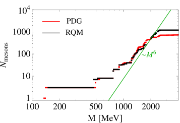
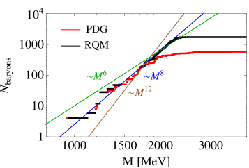
Figure 3: Cumulative numbers for the PDG (red line) and the RQM (black line). Left panel: mesonic states (log-log scale). Right panel: Baryonic states (log-log scale).

II Completeness and thermodynamic equivalence

II.1 QCD spectrum and thermodynamics

The cumulative number of states may be used as a characterization of the QCD spectrum Broniowski and Florkowski (2000); Broniowski et al. (2004). It is defined as the number of bound states below some mass $M$, i.e.

$$N(M)=\sum_{i}g_{i}\,\Theta(M-M_{i})\,,$$ (1)

where $g_{i}$ is the degeneracy factor, $M_{i}$ is the mass of the $i$-th hadron and $\Theta(x)$ is the step function, so that the density of states is given by $\rho(M)=dN(M)/dM$. A way to provide a practical meaning of the previous equation is to use finite box periodic (antiperiodic) boundary conditions for gluon/quark fields. In such a case all states contribute on equal footing. In such setting, stable bound states correspond to eigenvalues which do not depend on the volume of the box for sufficiently large boxes, whereas unstable resonance states correspond to eigenvalues which are volume independent within a given volume interval  Briceno et al. (2016). Colour neutral eigenstates of the QCD Hamiltonian and in fact excited states have been determined on the lattice in this way Edwards et al. (2013). Despite its importance, the cumulative number of states, Eq. (1) has never been evaluated directly in QCD.

Within a thermodynamic setup, the issue of completeness acquires a precise meaning where the global aspects of the spectrum rather than individual features are highlighted. The partition function of QCD is given by the standard relation

$$Z_{{\textrm{\scriptsize QCD}}}={\rm Tr}\,e^{-H_{{\textrm{\scriptsize QCD}}}/T}=\sum_{n}e^{-E_{n}/T}\,,$$ (2)

and is the fundamental quantity to study the thermodynamic properties of the theory. Written in terms of the eigenvalues of the QCD Hamiltonian, i.e. $H_{{\textrm{\scriptsize QCD}}}\psi_{n}=E_{n}\psi_{n}$, Eq. (2) illustrates the relation between the thermodynamics of the confined phase and the spectrum of QCD. Although $Z_{\rm QCD}$ has been determined independently as an Euclidean path integral on the lattice Borsanyi et al. (2012); Bazavov et al. (2012), to our knowledge the energy levels contribution to Eq. (2) has not been tested explicitly against the partition function. Actually, the primary quantity is the trace anomaly Borsanyi et al. (2012); Bazavov et al. (2012)

$$\Delta\equiv\frac{\epsilon-3P}{T^{4}}=T^{5}\partial_{T}\left(\frac{P}{T^{4}}\right)$$ (3)

whence the equation of state (EoS) can be obtained by integration of the rhs of this equation with suitable boundary conditions and physical quantities such as the entropy density $s=\partial_{T}P$ or the sound velocity $c_{s}^{2}=\partial P/\partial\epsilon\equiv\partial_{T}P/\partial_{T}\epsilon$ may be determined.

From this thermodynamic point of view it is fair to say that the completeness of the QCD-spectrum remains to be checked in practice.

II.2 Hadron Resonance Gas model: the PDG and RQM spectra

The completeness of the listed PDG states Patrignani et al. (2016) is equally a subtle issue. On the one hand they are mapped into the $q\bar{q}$ and $qqq$ quark model states. On the other hand, most reported states by the PDG are not stable particles but resonances which are produced as intermediate steps in a variety of scattering processes.

The HRG model was originally proposed by Hagedorn Hagedorn (1985). In spirit, this is valid under the assumption that physical quantities in the confined phase of QCD admit a representation in terms of hadronic states, which are considered as stable, non-interacting and point-like particles. Within this approach the EoS of QCD is described in terms of a gas of non-interacting hadrons Hagedorn (1985); Tawfik (2005), and the grand-canonical partition function turns out to be

$$\begin{split}\log Z_{\textrm{\scriptsize HRG}}&=-V\int\frac{d^{3}p}{(2\pi)^{3}}\sum_{i\in{\rm Hadrons}}\zeta_{i}g_{i}\\ &\quad\times\log\left(1-\zeta_{i}e^{-(\sqrt{p^{2}+M_{i}^{2}}-\sum_{a}\mu_{a}q_{a}^{i})/T}\right),\end{split}$$ (4)

with $\zeta_{i}=\pm 1$ for bosons and fermions respectively. We consider several conserved charges labeled by the index $a$, with $q_{a}^{i}$ the charge of the $i$-th hadron for symmetry $a$, and $\mu_{a}$ the chemical potential associated with this symmetry. The obvious consequence is that a good understanding of the spectrum of QCD turns out to be crucial for a precise determination of the thermodynamic properties of this theory.

In QCD, the quantized energy levels are the masses of low-lying and stable colour singlet states, which are commonly identified with mesons $[q\bar{q}]$ and baryons $[qqq]$ in the quark model. As already mentioned, unstable hadronic resonances are not proper eigenstates which in the HRG model are regarded as bound states. We reiterate that while there is currently a large scale on-going effort to determine hadronic resonances from lattice QCD by means of the Lüscher formula Edwards et al. (2013) (see e.g. Briceno et al. (2016) for a review) these states are not numerous enough to verify the HRG model.

So far, the states listed by PDG echo the standard quark model classification for mesons $[q{\bar{q}}]$ and baryons $[qqq]$. Then, it would be pertinent to consider also the Relativized Quark Model (RQM) for mesons Godfrey and Isgur (1985) and baryons Capstick and Isgur (1986). We show in Fig. 1 the hadron spectrum with the PDG compilation (left) and the RQM spectrum (right). The comparison clearly shows that there are further states in the RQM spectrum above some scale $M>M_{\min}$ that may or may not be confirmed in the future as mesons or hadrons. In addition there could be exotic, glueballs or hybrids states, predicted by other hadronic models.

The contribution to $N(M)$ obtained just adding the $q\bar{q}$ (mesons), $qqq$ (baryons) and $\bar{q}\bar{q}\bar{q}$ (antibaryons) components as 

$$N(M)=N_{[q{\bar{q}]}}(M)+N_{[qqq]}(M)+N_{[\bar{q}\bar{q}\bar{q}]}(M)\,,$$ (5)

can be evaluated either from the PDG booklet Patrignani et al. (2016) or alternatively from the RQM of Capstick, Godfrey and Isgur Godfrey and Isgur (1985); Capstick and Isgur (1986). The resemblance of both schemes below $1.7\,{\mathrm{GeV}}$, see Fig. 2 (left), is noteworthy, particularly if we take into account the 30 years elapsed between the RQM and the current PDG. Finite width effects on the PDG (PDG-$\Gamma$) have been estimated  Ruiz Arriola et al. (2012); Broniowski (2016) and naturally provide a shift towards lower masses as a consequence of the mass spectrum spread. The flattening of the curves indicates lack of reported states on the PDG side, as well as a the higher computational cut-off $M_{\rm high}=2.3\,{\mathrm{GeV}}$ in the numerical calculation on the RQM side.

This resemblance is also realized at the level of the trace anomaly which in the HRG model is given by

$$\Delta_{\rm HRG}(T)=\frac{1}{T^{4}}\sum_{i\in{\rm Hadrons}}\!\!g_{i}\int\frac{d^{3}p}{(2\pi)^{3}}\frac{E_{i}(p)-{\bm{p}}\cdot\nabla_{p}E_{i}(p)}{e^{E_{i}(p)/T}-\zeta_{i}}\,,$$ (6)

and compared with lattice QCD by the Wuppertal-Budapest (WB) and the HotQCD collaborations Borsanyi et al. (2014); Bazavov et al. (2014) in Fig. 2 (right), suggesting the thermodynamic equivalence of QCD, PDG and RQM below the crossover.

II.3 Missing states

Given the resemblance of the PDG to the RQM we may speculate on the nature of mesonic and baryonic states separately. While the PDG is a consented compilation of numerous analyses, the RQM corresponds by construction to a solution of the quantum mechanical problem for both $q\bar{q}$-mesons and $qqq$-baryons. For colour-singlet states the $n$-parton Hamiltonian takes the schematic form

$$H_{n}=\sum_{i=1}^{n}\sqrt{p_{i}^{2}+m^{2}}+\sum_{i<j}^{n}v_{ij}(r_{ij})\,.$$ (7)

Neglecting spin dependent contributions, not essential in the following argument, and assuming Casimir scaling, the two-body interactions take the form

$$v_{q\bar{q}}=\sigma r-\frac{4\alpha_{S}}{3r}=(N_{c}-1)v_{qq}\,.$$ (8)

Asymptotic estimates may be undertaken to sidestep the actual numerical evaluation of the eigenvalues. Specifically a semiclassical expansion describes the high mass spectrum for systems where interactions are dominated by linearly rising potentials with a string tension $\sigma$, in the range $M\gg\sqrt{\sigma}$. Such an approach relies on a derivative expansion of the cumulative number of states for a given Hamiltonian Caro et al. (1996). At leading order the number of states below a certain mass $M$ takes the form

$$N_{n}(M) \sim g_{n}\int\prod_{i=1}^{n}\frac{d^{3}x_{i}d^{3}p_{i}}{(2\pi)^{3}}\,\delta\!\!\left({\textstyle\sum_{i=1}^{n}{\bm{x}}_{i}}\right)\delta\!\!\left({\textstyle\sum_{i=1}^{n}{\bm{p}}_{i}}\right)$$ (9)

$$\times \theta(M-H_{n}(p,x))\,,$$

where $g_{n}$ takes into account the degeneracy.

For the sake of the argument, let us neglect the Coulomb term in (8), thus $v(r)=\sigma\,r$, as well as the current quark masses. In this case, a dimensional argument, $p\to Mp$, $r\to Mr/\sigma$, gives

$$N_{n}(M)\sim\left(\frac{M^{2}}{\sigma}\right)^{3n-3}.$$ (10)

Using these techniques, one can predict that the large mass expansion of these contributions is $N_{[q{\bar{q}}]}\sim M^{6}$, $N_{[qqq]}\sim M^{12}$, $N_{[q{\bar{q}}q{\bar{q}}]}\sim M^{18}\,,$ etc Ruiz Arriola et al. (2014).

The separate contributions of mesons and baryons are presented in Fig. 3 on a log-log scale where we see that again PDG and RQM largely agree and present an approximate linear behaviour on this scale, indicating as expected a power behaviour. However, while in the meson case the $N_{[q{\bar{q}}]}\sim M^{6}$ seems to conform with the asymptotic estimate, in the baryon case much lower powers, $M^{6}-M^{8}$, than the expected $N_{[qqq]}\sim M^{12}$ are identified. We note that $M^{6}$ suggests a similar two-body behavior as in the case of mesons (with a linearly rising potential). We take this feature as a hint that the $qqq$ excited spectrum effectively conforms to a two body system of particles interacting with a linearly growing potential, as we will analyze below in detail in Section V.2.

III Fluctuations of conserved charges in a thermal medium

While mesonic and baryonic contributions can be explicitly distinguished the thermodynamic separation of mesons and baryons in the EoS cannot be done at the QCD level. In order to achieve directly such a separation for baryons in particular we analyze fluctuations containing at least one baryonic charge as well as charge and strangeness, the three of them being conserved charges in strong interactions.

Conserved charges $[Q_{a},H]=0$ play a fundamental role in the thermodynamics of QCD. In the (uds) flavor sector of QCD the conserved charges are the electric charge $Q$, the baryon number $B$, and the strangeness $S$. While their thermal expectation values in the hot vacuum are vanishing, i.e. in the absence of chemical potentials  $\langle Q_{a}\rangle_{T}=0$, where $Q_{a}\in\{Q,B,S\}$, they present statistical fluctuations characterized by susceptibilities Bazavov et al. (2012); Bellwied et al. (2015); Asakawa and Kitazawa (2016); Ruiz Arriola et al. (2016)  

$$\chi_{ab}(T)\equiv\frac{1}{VT^{3}}\langle\Delta Q_{a}\Delta Q_{b}\rangle_{T}\,,\quad\Delta Q_{a}=Q_{a}-\langle Q_{a}\rangle_{T}\,.$$ (11)

The susceptibilities can be computed from the grand-canonical partition function by differentiation with respect to the chemical potentials, i.e.

$$\langle Q_{a}\rangle_{T}=-\frac{\partial\Omega}{\partial\mu_{a}}\,,\qquad\langle\Delta Q_{a}\Delta Q_{b}\rangle_{T}=-T\frac{\partial^{2}\Omega}{\partial\mu_{a}\partial\mu_{b}}\,,$$ (12)

where $\Omega=-T\log Z$ is the thermodynamical potential.

QCD at high temperature behaves as an ideal gas of quarks and gluons. In this limit the susceptibilities approach to

$$\chi_{ab}=\frac{N_{c}}{3}\sum_{i=1}^{N_{f}}q^{i}_{a}q^{j}_{b}\,;$$ (13)

hence for $N_{c}=3$ and flavors $u,d,s$

$$\begin{split}\chi_{BB}(T)&\to 1/3\,,\quad\!\!\!\!\!\!\chi_{BQ}(T)\to 0\,,\qquad\chi_{BS}(T)\to-1/3\,,\\ \chi_{SS}(T)&\to 1\,,\quad\;\,\chi_{QS}(T)\to 1/3\,,\quad\chi_{QQ}(T)\to 2/3\,.\end{split}$$ (14)

Within the HRG approach, the charges are carried by various species of hadrons, $Q_{a}=\sum_{i}q^{i}_{a}N_{i}$, where $q_{a}^{i}\in\{Q_{i},B_{i},S_{i}\}$, and $N_{i}$ is the operator number of hadrons of type $i$. By using in Eq. (12) the thermodynamic potential of this model, cf. Eq. (4), one gets

$$\begin{split}\chi_{ab}(T)=\frac{1}{2\pi^{2}}\sum_{i\in{\rm Hadrons}}\!\!g_{i}\,q_{i}^{a}\,q_{i}^{b}\sum_{n=1}^{\infty}\zeta_{i}^{n+1}\frac{M_{i}^{2}}{T^{2}}\,K_{2}\!\!\left(\frac{nM_{i}}{T}\right),\end{split}$$ (15)

where $K_{2}(z)$ refers to the Bessel function of the second kind. This formula will be used to compute the baryonic susceptibilities, namely $\chi_{BB}$, $\chi_{BQ}$ and $\chi_{BS}$. Eq. (15) predicts the asymptotic behavior

$$\chi_{ab}(T)\stackbin[T\to 0]{}{\sim}e^{-M_{0}/T}\,,$$ (16)

where $M_{0}$ is the mass of the lowest-lying state in the spectrum with quantum numbers $a$ and $b$. Therefore

$$\chi_{BB}(T)\stackbin[T\to 0]{}{\sim}e^{-M_{p}/T}\,,\quad\;\;\,\chi_{BQ}(T)\stackbin[T\to 0]{}{\sim}e^{-M_{p}/T}\,,$$ (17)

$$\chi_{BS}(T)\stackbin[T\to 0]{}{\sim}e^{-M_{\Lambda^{0}}/T}\,,\quad\,\,\chi_{SS}(T)\stackbin[T\to 0]{}{\sim}e^{-M_{K^{\pm}}/T}\,,$$

$$\chi_{QS}(T)\stackbin[T\to 0]{}{\sim}e^{-M_{K^{\pm}}/T}\,,\quad\chi_{QQ}(T)\stackbin[T\to 0]{}{\sim}e^{-M_{\pi^{\pm}}/T}\,,$$

where $M_{p}=938\,{\mathrm{MeV}}$ is the proton mass, $M_{\Lambda^{0}}$ the mass of the $\Lambda^{0}$ baryon, etc. These relations go beyond the HRG model, since for each sector the lightest hadron must certainly saturate the QCD partition function at low enough temperature. This observation makes it appealing to plot the lattice data for the fluctuations in a logarithmic scale. These plots are shown in Fig. 4.

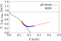
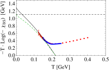
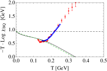
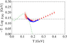
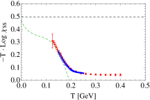
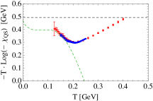
Figure 4: Plot of $-T\log|\chi_{ab}|$ as a function of temperature. We display as dots the lattice data from Refs. Bazavov et al. (2012) (blue) and Borsanyi et al. (2012) (red). We also display the HRG model results including the spectrum of the RQM Godfrey and Isgur (1985); Capstick and Isgur (1986) (dashed green) and the baryon spectrum from the quark-diquark model computed in Sec. V.2 (solid black). Horizontal dashed lines represent the values of the lowest-lying states contributing to the fluctuations, as it is shown in Eq. (17).

Of the six susceptibilities only four are independent, on account of isospin symmetry which requires $\chi_{uu}=\chi_{dd}$ and $\chi_{us}=\chi_{ds}$. On the other hand, the following inequality holds in QCD for degenerate $u,d$ flavors

$$\chi_{ud}(T)\leq 0\,,$$ (18)

at any temperature, even in the deconfined phase. This is proven in App. B. Because strange and light-quark flavors are not exactly degenerate, the relation $\chi_{us}(T)\leq 0$ does not follow as a QCD theorem but it is nevertheless supported by the lattice results.

In addition, the following relation holds for any pair of charges,

$$\chi_{aa}+\chi_{bb}\geq 2|\chi_{ab}|\,,$$ (19)

since $\langle(\Delta Q_{a}\pm\Delta Q_{b})^{2}\rangle$ is non-negative. In particular it follows

$$\chi_{uu}\geq-\chi_{ud}\geq 0\,.$$ (20)

The meson contribution to $\chi_{ud}$ is always negative while the baryon contribution is always positive. The negative global result indicates that mesons dominate over baryons in $\chi_{ud}$. Going to low temperatures, this provides yet another proof that in QCD with two degenerate light flavors the lightest meson is lighter than the lightest baryon. We display in Fig. 5 some of these relations for the lattice data of the susceptibilities, and check that they are fulfilled.

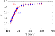
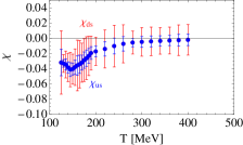
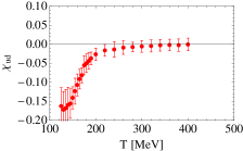
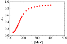
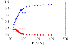
Figure 5: Plot of the susceptibilities $\chi_{ab}$ in the quark-flavor basis as a function of temperature. The dots are the lattice data from Ref. Borsanyi et al. (2012). We are checking numerically in these plots the relations Eqs. (18)-(20). Similar results are obtained with the lattice data of Ref. Bazavov et al. (2012).

Finally, let us mention that higher order fluctuations can be obtained within the HRG model by taking higher derivatives of the thermodynamics potential. This leads to

$$\begin{split}\chi^{BQS}_{pqr}(T)&=\frac{1}{2\pi^{2}}\sum_{i\in{\rm Hadrons}}g_{i}\,B_{i}^{p}Q_{i}^{q}S_{i}^{r}\\ &\quad\times\sum_{n=1}^{\infty}\zeta_{i}^{n+1}n^{p+q+r-2}\,\frac{M_{i}^{2}}{T^{2}}K_{2}\!\left(\frac{nM_{i}}{T}\right).\end{split}$$ (21)

Some results of fourth-order fluctuations are presented in Section V.3.

IV Quark-diquark potential from Polyakov loop correlators

In view of the missing resonance problem alluded to previously there is nowadays some discussion about the most probable spatial configuration of quarks inside baryons, and more specifically the structure of excited states. In the quark model such as the RQM Godfrey and Isgur (1985); Capstick and Isgur (1986) baryons are $qqq$ states where the interaction is given by a combination of $\Delta$-like pairs of $qq$ interactions and a genuinely $Y$-like $qqq$ interaction. Remarkably the $Y$-stringlike behavior of a static baryon energy at finite temperature has been observed in Ref. Bakry et al. (2015). An interesting possibility would be that the quarks are distributed according to an isosceles triangle. This is the idea behind an easily tractable class of models, the so-called relativistic quark-diquark ($qD$) models with non-relativistic Santopinto (2005) and relativistic Ferretti et al. (2011); Gutierrez and De Sanctis (2014) variants where a linearly rising potential is shown to work phenomenologically. In addition to this success, there was no further reason to invoke such a behaviour. In the next paragraphs we elaborate on this and provide a theoretical argument in favor of the presence of a linear potential.

It should be noted that by definition, a potential can only be evaluated unambiguously (up to an additive constant) in the heavy particles or static limit, since then the position operator is well defined. The calculation of $qD$ static interactions for heavy sources has been addressed on the lattice in several works Bissey et al. (2009); Bakry et al. (2018); Koma and Koma (2017), where it has actually been found that up to numerical uncertainties the potential is linearly rising, and the corresponding string tension is numerically identical to the one of the $q\bar{q}$ system (see specifically Ref. Koma and Koma (2017)). In this section we show analytically that under very specific assumptions this must actually be true. To show how this comes about we will rely heavily on our previous work on free energies Megias et al. (2014) where a more detailed discussion can be found. Here we just summarize the main issues relevant to the problem at hand.

An operational way of placing static sources in a gauge theory such as QCD, is by introducing in the Euclidean formulation a local gauge rotation $\Omega$ realized by the Polyakov loop, i.e., the gauge covariant operator defined as

$$\Omega({\bm{x}})=P\,e^{\,i\int_{0}^{\beta}A_{0}(x)\,dx_{0}},$$ (22)

where $P$ indicates path ordering and $A_{0}$ and $x$ are Euclidean. The colour source may be decomposed into irreducible representations, say $\mu$ so that one can build the gauge invariant combinations corresponding to the character in that representation, $\chi_{\mu}[\Omega(x)]$. For instance, the trace in the (anti)fundamental representation corresponds to the character of the ${\mathrm{SU}}(3)$ colour gauge group,

$${\rm tr}\,\Omega({\bm{x}})\equiv\chi_{\bf 3}[\Omega({\bm{x}})]\,,\qquad{\rm tr}\,\Omega({\bm{x}})^{\dagger}\equiv\chi_{\bf 3}[\Omega({\bm{x}})]^{*}\,.$$ (23)

Thus, the $q\bar{q}$ free energy is given by a thermal expectation value

$$e^{-F_{q\bar{q}}(r,T)/T}=\langle{\rm tr}\,\Omega({\bm{x}}_{1}){\rm tr}\,\Omega({\bm{x}}_{2})^{\dagger}\rangle_{T}$$ (24)

where due to translational invariance the free energy depends only on the separation $r=|{\bm{x}}_{1}-{\bm{x}}_{2}|$. In this and the following expressions, an ambiguity of an additive constant must be allowed in the free energies coming from the renormalization of the Polyakov loop operator. The potential is obtained as the zero temperature limit of the free energy

$$V_{q\bar{q}}(r)=F_{q\bar{q}}(r,0)\,.$$ (25)

Likewise the $qqq$ free energy is given by

$$e^{-F_{qqq}({\bm{x}}_{1},{\bm{x}}_{2},{\bm{x}}_{3},T)/T}=\langle{\rm tr}\,\Omega({\bm{x}}_{1}){\rm tr}\,\Omega({\bm{x}}_{2}){\rm tr}\,\Omega({\bm{x}}_{3})\rangle_{T}\,.$$ (26)

In the limit ${\bm{x}}_{3}\to{\bm{x}}_{2}$ we get, for the quark-diquark free energy

$$e^{-F_{qD}({\bm{x}}_{1},{\bm{x}}_{2},T)/T}=\langle{\rm tr}\,\Omega({\bm{x}}_{1}){\rm tr}(\Omega({\bm{x}}_{2})^{2})\rangle_{T}\,.$$ (27)

This limit is singular since at very small distances the interaction is dominated by one gluon exchange, $\sim 1/r$, and a self-energy must be added. The renormalization of the new composite operator ${\rm tr}(\Omega({\bm{x}}_{2})^{2})$ yields a new ambiguity in the form of an additive constant from $F_{qqq}({\bm{x}}_{1},{\bm{x}}_{2},{\bm{x}}_{2},T)$ to $F_{qD}({\bm{x}}_{1},{\bm{x}}_{2},T)$.

Using the Clebsch-Gordan series

$${\bf 3}\otimes{\bf 3}={\bf\bar{3}}\oplus{\bf 6}\,,$$ (28)

yields the equivalent character relations

$$[\chi_{\bf 3}]^{2}=\chi_{\bf\bar{3}}+\chi_{\bf 6}\,,$$ (29)

and therefore

$$e^{-F_{qD}({\bm{x}}_{1},{\bm{x}}_{2},T)/T}\equiv e^{-F_{q\bar{q}}({\bm{x}}_{1},{\bm{x}}_{2},T)/T}+e^{-F_{6\otimes 3}({\bm{x}}_{1},{\bm{x}}_{2},T)/T}.$$ (30)

The $qD$ potential is obtained in the zero temperature limit. In this limit we expect the energy ${\bf 6}\otimes{\bf 3}$ configuration to be larger than that of the $q\bar{q}$ one, hence

$$V_{qD}(r)=V_{q\bar{q}}(r)+{\rm const}\,.$$ (31)

V Quark-diquark model for the baryon

V.1 The model Hamiltonian

In these models, the baryons are assumed to be composed of a constituent quark, $q$, and a constituent diquark, $D\equiv(qq)$ Santopinto and Ferretti (2015), and the Hamiltonian writes 

$$H_{qD}=\sqrt{{\bm{p}}^{2}+m_{q}^{2}}+\sqrt{{\bm{p}}^{2}+m_{D}^{2}}+V_{qD}(r)\,.$$ (32)

In Sec. IV we have argued that the quark-diquark potential is the same as the quark-antiquark potential, up to an additive constant. For the latter we assume $V_{q{\bar{q}}}(r)=-\frac{\tau}{r}+\sigma r+c$, hence

$$V_{qD}(r)=-\frac{\tau}{r}+\sigma r+\mu\,,$$ (33)

with $\sigma=(0.42\,{\mathrm{GeV}})^{2}$. In addition, we adopt the value $\tau=\pi/12$, as expected from the Lüscher term in the potential Luscher (1981).

In this model we can distinguish between two kinds of diquarks: scalar, $D$, and axial-vector, $D_{AV}$. When considering the quark content notation of a diquark, we will use $[q_{1}q_{2}]$ to denote scalar diquarks, and $\{q_{1}q_{2}\}$ for axial-vector diquarks. Some studies on QCD indicate that the mass difference between these diquarks is Jaffe (2005)

$$\Delta m_{D}:=m_{D_{AV}}-m_{D}\simeq 0.21\,{\mathrm{GeV}}\,.$$ (34)

In what follows we adopt this value for $\Delta m_{D}$. We will assume that the mass parameters of the model are controlled by a constituent quark mass, $m_{\textrm{\scriptsize cons}}$, and the current quark mass for the strange quark, $\hat{m}_{s}$, in the following way:

$$m_{u,d}=m_{\textrm{\scriptsize cons}}\,,\qquad m_{s}=m_{\textrm{\scriptsize cons}}+\hat{m}_{s}\,.$$ (35)

The breaking of flavor ${\mathrm{SU}}(3)$ for diquarks will be modeled as

$$m_{D}=m_{D,\textrm{{ns}}}+n_{s}\hat{m}_{s}\,,$$ (36)

where $m_{D,\textrm{{ns}}}$ is the scalar mass of non strange diquarks, and $n_{s}=0,1,2,$ is the number of $s$-quarks in the diquark. The further choice

$$m_{D,\textrm{{ns}}}=2m_{{\textrm{\scriptsize cons}}}$$ (37)

is rather natural, but we will not always enforce it.

With these assumptions, the only free parameters of the model are $m_{\textrm{\scriptsize cons}}$, $\hat{m}_{s}$ and $\mu$, plus $m_{D,\textrm{{ns}}}$ if (37) is not enforced. The goal is to reproduce the lattice results for the baryonic fluctuations $\chi_{BB}$, $\chi_{BQ}$ and $\chi_{BS}$ for temperatures below the crossover. For the baryonic states $B=1$ and $S=-n_{s}$. The electric charges and the degeneracies of the states are summarized in Table 1. The spectrum is computed as explained below. With these ingredients the susceptibilities can be evaluated in the model using Eq. (15).

Baryon	Total deg.	$Q=-1$	$Q=0$	$Q=1$	$Q=2$
$[nn]n$	4	-	2	2	-
$\{nn\}n$	36	6	12	12	6
$[nn]s$	2	-	2	-	-
$\{nn\}s$	18	6	6	6	-
$[ns]n$	8	2	4	2	-
$\{ns\}n$	24	6	12	6	-
$[ns]s$	4	2	2	-	-
$\{ns\}s$	12	6	6	-	-
$\{ss\}n$	12	6	6	-	-
$\{ss\}s$	6	6	-	-	-

Table 1: Spin-isospin degeneracies of the baryonic states within the quark-diquark model of Sec. V. The second column contains the total degeneracy of each state, while the columns from $Q=-1$ to $Q=2$ contain the degeneracies by distinguishing between the electric charges of the states. $n$ represents the light flavors $u,d$.

V.2 Baryon spectrum

In order to obtain the baryon spectrum with the quark-diquark model we have to diagonalize the Hamiltonian of Eq. (32). Since the problem does not admit a closed analytic solution we will obtain the spectrum numerically after truncation to a model space and diagonalization of the corresponding finite dimensional matrix. This is a variational procedure. Because of the form of the Hamiltonian $H=f_{1}(p)+f_{2}(r)$ a convenient basis is that of the isotropic harmonic oscillator, with normalized wave functions of the form

$$R_{nl}(r)=\frac{e^{-\frac{r^{2}}{2b^{2}}}}{\sqrt[4]{\pi}}\!\left(\frac{r}{b}\right)^{l}\!\sqrt{\frac{(n-1)!\,2^{l+n+1}}{b^{3}(2l+2(n-1)+1)!!}}L_{n-1}^{l+\frac{1}{2}}\!\left(\frac{r^{2}}{b^{2}}\right)\,.$$ (38)

$L_{n-1}^{l+\frac{1}{2}}(x)$ are the generalized Laguerre polynomials and the positive parameter $b$ is related to the oscillator mass and frequency. $b$ can be optimized as a variational parameter. The reduced wave functions $u_{nl}(r)$ are normalized to unity

$$u_{nl}(r)=r\,R_{nl}(r),\qquad\int_{0}^{\infty}dr\,u_{nl}(r)^{2}=1\,.$$ (39)

The corresponding wave functions in momentum space, $\hat{R}_{nl}(p)$, have the same form as those in Eq. (38) up to a phase and $b\to 1/b$, namely

$$\hat{u}_{nl}(p;b)=(-i)^{l+2n-2}u_{nl}(p;1/b).$$ (40)

Then the matrix elements $\langle nl|H_{qD}|n^{\prime}l\rangle$ are obtained from

$$\langle nl|H_{qD}|n^{\prime}l\rangle =\int_{0}^{\infty}dp\,\hat{u}_{nl}^{\ast}(p)\hat{u}_{n^{\prime}l}(p)\left[\sqrt{p^{2}+m_{q}^{2}}+\sqrt{p^{2}+m_{D}^{2}}\right]$$ (41)

$$\quad+\int_{0}^{\infty}dr\,u_{nl}^{\ast}(r)u_{n^{\prime}l}(r)V_{qD}(r)\,,$$

with $n=1,\dots,n_{\max}$, and $l=0,\dots,l_{\max}$. The value of the parameter $b$ is fixed to minimize the averaged value of the energy levels in the spectrum for each of the multiplets in Table 1. Typical values of this parameter are in the range $0.55\,{\mathrm{fm}}\lesssim b\lesssim 0.65\,{\mathrm{fm}}$.

We display in Fig. 6 the dependence of the mass of the baryonic state, $\Lambda^{0}$, as a function of $n_{\max}$, taking $l_{\max}=n_{\max}-1$. We can see that the dependence on $n_{\max}$ is very weak already for $n_{\max}=4$. We have cross-checked many of the results presented subsequently by including larger values of $n_{\max}$ and $l_{\max}$, and we find that they do not change appreciably.

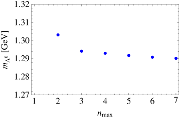
Figure 6: Mass of the baryonic state, $\Lambda^{0}$, as a function of $n_{\max}$ from diagonalization of Eq. (41) with the parameters in (42).

After considering a convenient choice of the parameters of the model, for instance

$$m_{D,\textrm{{ns}}}=0.6\,{\mathrm{GeV}}\,,\quad m_{u,d}=0.3\,{\mathrm{GeV}}\,,$$ (42)

$$\hat{m}_{s}=0.10\,{\mathrm{GeV}}\,,\quad\mu=-0.459\,{\mathrm{GeV}}\,,$$

and following the procedure mentioned above, we get the spectrum of baryons that is shown in Fig. 7. In this figure we compare this result to the RQM spectrum Capstick and Isgur (1986) on a log-log plot where the $\sim M^{6}$ growth of the quark-diquark baryonic spectrum can be clearly identified. It is quite remarkable that below $M<2400\,{\mathrm{MeV}}$ the quark-diquark spectrum is in good agreement with the RQM spectrum. While the authors of Ref. Capstick and Isgur (1986) do not compute baryon masses heavier than this, with the present quark-diquark model we have obtained further states up to $M\approx 3400\,{\mathrm{MeV}}$. Within the HRG picture, these states will contribute to the EoS of QCD as well as to other thermal observables like the fluctuations. The choice of parameters of Eq. (42) is motivated by a comparison with the lattice results for the thermal fluctuations, as we will see in the next section.

Let us mention that, unless otherwise stated, in the following we will use the empirical value of the mass for the nucleon, $M_{n}=938\,{\mathrm{MeV}}$, and apply the quark-diquark model only for the other baryons. The effect of using the empirical mass for all the baryons in the $1/2^{+}$ octet is also discussed. The justification for this is that it is expected that the quark-diquark picture will be reliable only for excited states. As we will show in the next subsection, this is confirmed from the analysis of the lattice data for the baryonic fluctuations.

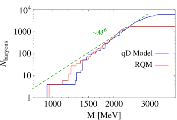
Figure 7: Cumulative number for the spectrum of baryons as a function of the mass in a log-log plot comparing the RQM Capstick and Isgur (1986), and the quark-diquark model used in this paper. We have used the parameters in Eq. (42). We also draw the $\sim M^{6}$ line for illustration.

V.3 Baryonic fluctuations

From the spectrum of the quark-diquark model, we can obtain the baryonic fluctuations by using the HRG approach given by Eq. (15). Our goal is to reproduce the lattice results for these quantities, at least for the lowest temperature values. A typical fit of the model prediction with lattice data is shown in Fig. 8. While ideally one would like to have temperatures as low as possible so as to determine in a clean way the low-lying states with the proper quantum numbers, in practice we find that at the lowest available temperatures, the contribution of excited states becomes individually small but collectively important. This is a typical problem in intermediate temperature analyses, and this is the reason why all possible constraints on the model, such as the identity of quark-diquark and quark-antiquark potentials discussed above, are particularly welcome.

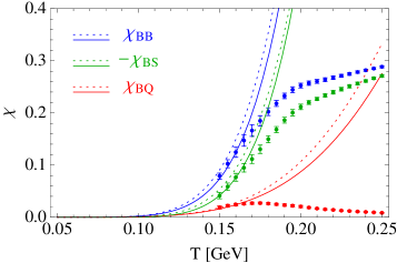
Figure 8: Baryonic susceptibilities from the quark-diquark model (solid) compared to the lattice data of Ref. Bazavov et al. (2012). We have used the parameters in Eq. (42). We display also as dotted lines the result from the spectrum of the RQM Capstick and Isgur (1986).

In order to perform the best fit to the data, we have chosen to minimize the function

$$\bar{\chi}^{2}=\bar{\chi}_{BB}^{2}+\bar{\chi}_{BQ}^{2}+\bar{\chi}_{BS}^{2}\,,$$ (43)

where

$$\bar{\chi}_{ab}^{2}=\sum_{j=1}^{j_{\max}}\frac{\left(\chi_{ab}^{{\textrm{\scriptsize lat}}}(T_{j})-\chi_{ab}^{\textrm{\scriptsize HRG}}(T_{j})\right)^{2}}{(\Delta\chi_{ab}^{{\textrm{\scriptsize lat}}}(T_{j}))^{2}}\,.$$ (44)

Here the $T_{j}$ are the temperatures used in the lattice calculations. The lowest temperature of the data is $T_{1}=125\,{\mathrm{MeV}}$ for Ref. Borsanyi et al. (2012) and $T_{1}=150\,{\mathrm{MeV}}$ for Ref. Bazavov et al. (2012), while $j_{\max}$ is the number of data points used in the fit for each of the susceptibilities. $\Delta\chi_{ab}^{{\textrm{\scriptsize lat}}}$ are the uncertainties of the lattice results.

Since a hadronic model is not expected to reproduce the QCD crossover we fit the data corresponding to the lower temperatures in lattice measurements. Statistical considerations Ruiz Arriola et al. (2018) indicate that those data points should be included for which

$$1-\sqrt{\frac{2}{\nu}}<\frac{\bar{\chi}^{2}}{\nu}<1+\sqrt{\frac{2}{\nu}}\,,$$ (45)

where $\nu$ is the number of degrees of freedom. This condition fixes our choice of $j_{\max}$. In our case, $\nu=n_{\rm obs}j_{\max}-n_{{\textrm{\scriptsize param}}}$, with $n_{\rm obs}=3$ since three baryonic fluctuations are being fitted, and $n_{{\textrm{\scriptsize param}}}$ is the number of free parameters of the model.

The fits turn out to be very sensitive to the parameter $\mu$ in Eq. (33); hence it is convenient to always minimize $\bar{\chi}^{2}$ with respect to this parameter. Whenever we provide or plot a value for the function $\bar{\chi}^{2}/\nu$, it should be understood that this function is already minimized with respect to the parameter $\mu$. Typical values of this parameter are $-0.7\,{\mathrm{GeV}}\lesssim\mu\lesssim 0\,{\mathrm{GeV}}$.

As a first step in the analysis, we show in Fig. 9 a plot of $\bar{\chi}^{2}/\nu$ as a function of the current quark mass, while fixing the constituent mass to $m_{{\textrm{\scriptsize cons}}}=0.3\,{\mathrm{GeV}}$ and $m_{D,\textrm{{ns}}}=2m_{{\textrm{\scriptsize cons}}}$. When including in the fits only the lowest temperature point of the data, i.e. $j_{\max}=1$, one gets an exceedingly good fit with $\bar{\chi}^{2}/\nu=1.0\times 10^{-4}$ for $\hat{m}_{s}=0.130\,{\mathrm{GeV}}$. This is rather surprising, as it means that three central values of the data can be fitted almost exactly with just two parameters: $\hat{m}_{s}$ and $\mu$. The fit deteriorates but it is still acceptable when the four lowest temperatures are used, $j_{\max}=4$. We find that the model and the lattice data are compatible with Eq. (45) for temperatures $T\lesssim 165\,{\mathrm{MeV}}$, either if we analyze the lattice data of Ref. Borsanyi et al. (2012) or Bazavov et al. (2012). The best fit in this case with $\bar{\chi}^{2}/\nu=0.68$ is for $\hat{m}_{s}=0.099\,{\mathrm{GeV}}$ and $\mu=-0.459\,{\mathrm{GeV}}$.

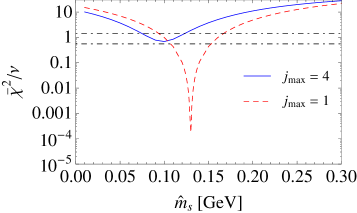
Figure 9: $\bar{\chi}^{2}/\nu$ as a function of $\hat{m}_{s}$ with $m_{{\textrm{\scriptsize cons}}}=0.3\,{\mathrm{GeV}}$, and $m_{D,\textrm{{ns}}}=2m_{{\textrm{\scriptsize cons}}}$. The dashed red line corresponds to $j_{\max}=1$ while the solid blue line corresponds to $j_{\max}=4$. The horizontal lines correspond to the upper and lower bounds of Eq. (45). We have used the lattice data of Ref. Bazavov et al. (2012).

Fig. 10 shows plots of $\bar{\chi}^{2}/\nu$ in two versions. The left panel corresponds to the plane $(\hat{m}_{s},m_{{\textrm{\scriptsize cons}}})$ with $m_{D,\textrm{{ns}}}=2m_{{\textrm{\scriptsize cons}}}$, while the right panel corresponds to the plane $(m_{D,\textrm{{ns}}},m_{{\textrm{\scriptsize cons}}})$ with $\hat{m}_{s}=0.10\,{\mathrm{GeV}}$.

The left panel clearly indicates that the current quark mass takes a value compatible with the PDG, i.e. $80\,{\mathrm{MeV}}\lesssim\hat{m}_{s}\lesssim 120\,{\mathrm{MeV}}$. In addition, the value of the constituent quark mass cannot be determined with precision, but at least we can ensure that it is in the regime $100\,{\mathrm{MeV}}\lesssim m_{{\textrm{\scriptsize cons}}}\lesssim 400\,{\mathrm{MeV}}$.

In the right panel we have fixed $\hat{m}_{s}=0.10\,{\mathrm{GeV}}$, and used the scalar mass of non strange diquarks, $m_{D,\textrm{{ns}}}$, as a free parameter. The figure shows that the most probable scalar diquark mass is of the order of $m_{D,\textrm{{ns}}}\simeq 0.4-0.5\,{\mathrm{GeV}}$ and the mass of the constituent quarks $m_{{\textrm{\scriptsize cons}}}\simeq 0.3\,{\mathrm{GeV}}$. However, these values depend of the choice of the current quark mass, so that when increasing the value of $\hat{m}_{s}$, the best fits happen for lower values of $m_{{\textrm{\scriptsize cons}}}$. For instance, for $\hat{m}_{s}=0.12\,{\mathrm{GeV}}$ the best fit is obtained when $m_{{\textrm{\scriptsize cons}}}\lesssim 0.2\,{\mathrm{GeV}}$, while for $\hat{m}_{s}=0.09\,{\mathrm{GeV}}$ one obtains values $m_{{\textrm{\scriptsize cons}}}\simeq 0.5-0.6\,{\mathrm{GeV}}$.

As mentioned above, for our fits we have taken the value of the PDG for the nucleon mass, $M_{n}=938\,{\mathrm{MeV}}$, and used the quark-diquark model values for the remaining baryonic states. One could further adopt the empirical values for the masses of the $1/2^{+}$ baryonic octet, that is, $M_{\Lambda^{0}}=1.116\,{\mathrm{GeV}}$, $M_{\Sigma}=1.193\,{\mathrm{GeV}}$, and $M_{\Xi}=1.318\,{\mathrm{GeV}}$, in view of the fact that they are stable under strong interactions. Such states correspond to 16 of the 18 states of the type $[qq]q$ in Table 1. Specifically $N$, $\Sigma$ and $\Xi$ correspond to $[nn]n$, $[ns]n$ and $[ns]s$. The four remaining states in $[nn]s$ and $[ns]n$ correspond to the $\Lambda^{0}$ of the octet plus an ${\rm SU}(3)$ singlet $\Lambda$-like state Santopinto and Ferretti (2015). Since the mass of $[nn]s$ is slightly lighter than $[ns]n$ we assign the $\Lambda^{0}$ to this multiplet; the opposite assignation produces very similar results. The effect of using the empirical masses for the whole octet is that the best fits presented in Figs. 9 and 10 (left) are shifted to larger values of $\hat{m}_{s}$, namely $\Delta\hat{m}_{s}\simeq 24\,{\mathrm{MeV}}$. The quality of the fits is similar.

The value of the nucleon mass as predicted by our version of the quark-diquark model is $M_{n}\simeq 1.16\,{\mathrm{GeV}}$. If this value is used instead of the empirical one, the fits to the susceptibilities worsen. We show in Fig. 11 a plot of $\bar{\chi}^{2}/\nu$ in the plane $(\hat{m}_{s},m_{{\textrm{\scriptsize cons}}})$ using the nucleon mass as given by the model. One can see that in this case the best fits would correspond to non physical values of the current strange-quark mass, $150\,{\mathrm{MeV}}\lesssim\hat{m}_{s}\lesssim 220\,{\mathrm{MeV}}$.

In our model, as in other quark models such as that of Capstick and Isgur Capstick and Isgur (1986), we have assumed that the string tension for the light quarks coincides with the one obtained from heavy quarks, and hence for the qD system we have taken $\sigma=(0.42\,{\mathrm{GeV}})^{2}$. There are models where this value is reduced by a factor of 2 when discussing baryon spectroscopy, as good spectra are obtained for $(u,s,d)$ with $\sigma_{qD}=2.15\,{\mathrm{fm}}^{-2}$ Ferretti et al. (2011), for $(u,d)$ $\sigma_{qD}=1.57\,{\mathrm{fm}}^{-2}$De Sanctis et al. (2016) and for $(c,b)$ with $\sigma_{qD}=4.5\,{\mathrm{fm}}^{-2}$ Ebert et al. (2011). We note in passing that this factor of two re-scaling is also needed in the slope of radial Regge trajectories Ruiz Arriola and Broniowski (2007). Motivated by these observations we have repeated our analysis taking $\sigma=(0.42\,{\mathrm{GeV}})^{2}/2$, with minor modifications but slightly worse fit quality.

We have studied as well the baryonic fluctuations of fourth order. Fig. 12 shows the results for $\chi_{4}^{B}$, $\chi_{22}^{BQ}$, $\chi_{31}^{BQ}$ and $\chi_{121}^{BQS}$, computed from the quark-diquark model and RQM model by using Eq. (21), and compared with lattice data from Ref. Borsanyi et al. (2018). It can be noted that while the agreement is reasonable, these lattice data are typically affected by larger error bars than those of the second order fluctuations studied above, and the behavior of the data turn out to be noisier, hence no firm conclusions can be extracted from a fit to these quantities.

Finally, let us stress at this point that the lattice data used in the present study might have strong correlations. Besides correlations between susceptibilities at a single temperature, the data at different temperatures could also be correlated as a consequence of the reweighting technique and interpolations used in the lattice simulations. These correlations could modify the results of the fit and values of $\bar{\chi}^{2}$. Unfortunately, to our knowledge numerical data on such correlations are not available, so such analysis is not possible at present.

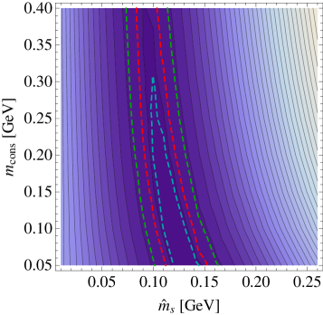
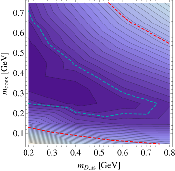
Figure 10: $\bar{\chi}^{2}/\nu$ from a fit to the lattice data of the baryonic fluctuations from Ref. Bazavov et al. (2012) with $j_{\max}=4$. The dashed lines correspond to $\bar{\chi}^{2}/\nu=0.77$ (blue), $\bar{\chi}^{2}/\nu=1$ (red) and $1+\sqrt{2/\nu}$ (green). $\mu$ is determined from minimization. Left panel: plane $(\hat{m}_{s},m_{{\textrm{\scriptsize cons}}})$ as free parameters with $m_{D,\textrm{{ns}}}=2m_{{\textrm{\scriptsize cons}}}$. Right panel: plane $(m_{D,\textrm{{ns}}},m_{{\textrm{\scriptsize cons}}})$ with $\hat{m}_{s}=0.10\,{\mathrm{GeV}}$.

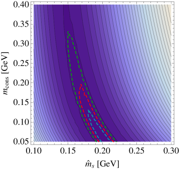
Figure 11: $\bar{\chi}^{2}/\nu$ in the plane $(\hat{m}_{s},m_{{\textrm{\scriptsize cons}}})$ from a fit to the lattice data of the baryonic fluctuations from Ref. Bazavov et al. (2012) with $j_{\max}=4$, and using the value of the nucleon mass as obtained from the quark-diquark model. The dashed lines correspond to $\bar{\chi}^{2}/\nu=1.275$ (blue), $\bar{\chi}^{2}/\nu=1.35$ (red) and $1+\sqrt{2/\nu}$ (green).

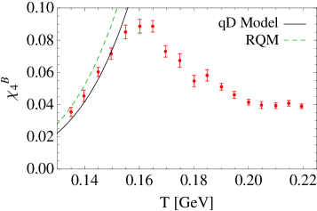
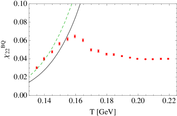
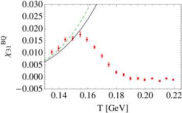
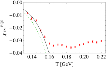
Figure 12: Baryonic susceptibilities of fourth order, $\chi_{4}^{B}$, $\chi_{22}^{BQ}$, $\chi_{31}^{BQ}$ and $\chi_{121}^{BQS}$, from the quark-diquark model (solid black) compared to the lattice data of Ref. Borsanyi et al. (2018). We have used the parameters in Eq. (42). We display also as dashed green lines the result from the spectrum of the RQM Capstick and Isgur (1986).

VI Conclusions

The missing resonance problem, i.e., the apparent overcounting of excited baryonic states by the quark model compared to the experimentally found resonances has been a long standing puzzle which has motivated a wealth of theoretical analysis and experimental work, mainly grounded in the individual identification of resonance states in the production process. This viewpoint demands a good knowledge of the scattering amplitude and its analytical properties in the complex energy plane. Indeed, resonances are uniquely characterized as process-independent complex energy poles in unphysical sheets but the extrapolation from the physical axis, where measurements are actually made, to the complex plane is subjected to potentially large uncertainties due to the role played by the background.

The thermodynamic approach to the missing states problem for baryons has several advantages over the more conventional individual states analysis, since it addresses the completeness of states problem from the point of view of quark-hadron duality. It is rather insensitive to resonance energy profiles as fine details of the level density are washed by the Boltzmann factor. Lattice QCD has produced thermodynamic quantities, such as the trace anomaly, where with the currently rather small uncertainties one is not able to tell the difference between the current PDG spectrum and a quark model spectrum such as the RQM which was inferred already a few decades ago. Differences in the comparison become more visible when susceptibilities involving baryon number, electric charge and strangeness are considered as different subsets of states are selected.

For zero density, conserved charges such as $B,Q,S$ have zero expectation values but fluctuate statistically in a hot vacuum. Those fluctuations are characterized by susceptibilities that have been determined numerically in QCD on the lattice by the HotQCD and WB Collaborations to discriminate among hadronic models with sufficient accuracy, and thus can be used as a benchmark comparison.

We have argued that the asymptotic three-body phase space for confined $qqq$ systems $\sim M^{12}$ is much larger than the one actually determined in RQM $\sim M^{6}$ which resembles instead a two body system with a linearly growing potential. This strongly suggests a dominance of quark-diquark dynamics for excited baryons. Therefore, we have considered a quark-diquark model with a linearly confining interaction.

By analyzing the free energy of heavy quark sources characterized by Polyakov loops, we have been able to disclose under what conditions the poorly known quark-diquark string tension should coincide with the much familiar quark-antiquark string tension, in agreement with previous and recent lattice results.

Using this a priori fixed quark-diquark potential we have determined the remaining model parameters from conserved charges susceptibilities. The results are reasonable and fall in the bulk of previous intensive studies where a detailed description of the spectrum was pursued.

Finally, let us mention that the study of nonbaryonic susceptibilities would require a specific model for mesons which, in principle, would not be related to the quark-diquark dynamics exploited in this manuscript. Such study is worth pursuing but goes beyond the scope of the present analysis.

Appendix A WKB estimates of the susceptibilities

In this appendix we compute the susceptibilities within a semiclassical expansion. Eq. (15) can be expressed as

$$\chi_{ab}(T)=\sum_{\zeta=\pm}\int_{0}^{\infty}dM\rho^{\zeta}_{ab}(M)\Phi_{\zeta}(M/T)$$ (46)

where

$$\Phi_{\zeta}(z)=\frac{z^{2}}{2\pi^{2}}\sum_{k=1}^{\infty}\zeta^{k+1}K_{2}(kz)$$ (47)

and

$$\rho^{\zeta}_{ab}(M)=\sum_{i}g_{i}q_{i}^{a}q_{i}^{b}\delta(M-M_{i})\,,$$ (48)

and the sum is over mesons or baryons for $\zeta=\pm$, respectively.

For the baryonic susceptibility $\chi_{BB}$, which is the case we are going to consider in the following, $\rho_{BB}(M)$ is equal to the density of states $\rho(M)$, as $B=\pm 1$ for (anti)baryons. The density of states can by computed in a derivative expansion Caro et al. (1996), an approximation that is closely related to a semiclassical expansion in the high mass spectrum. In this approach it is best to start from the cumulative number

$$N(M)={\rm Tr}(\Theta(M-\hat{H}))$$ (49)

where $\hat{H}$ is the Hamiltonian and the trace is taken in the center of mass system subspace. The density is then obtained from $\rho(M)=dN(M)/dM$.

In the quark-diquark model, the space of states is divided in sectors, $\lambda$, shown in Table 1. Each sector contains a tower of multiplets all with degeneracy $g_{\lambda}$ displayed in the Table. This gives

$$N(M)=\sum_{\lambda}g_{\lambda}N^{(\lambda)}(M)$$ (50)

where the sum is over sectors and $N^{(\lambda)}(M)$ sums over the tower of states including just one state in each multiplet. For the sake of clarity, in what follows we will drop the label $\lambda$. It is understood that the aggregated expressions are obtained by combining the results of the various sectors as in Eq. (50).

Within the semiclassical expansion, the cumulative number can be computed as

$$N(M)=\int\frac{d^{3}xd^{3}p}{(2\pi)^{3}}\Theta(M-H)+\cdots\,,$$ (51)

where $H$ is the (classical) Hamiltonian of the two-body system in the sector $\lambda$. The zeroth order term has been made explicit while the dots stand for higher order contributions in the derivative expansion.

The Hamiltonian takes the form

$$H=\sqrt{{\bm{p}}^{2}+m_{q}^{2}}+\sqrt{{\bm{p}}^{2}+m_{D}^{2}}+\sigma r-\frac{4\alpha_{S}}{3r}+\mu\,,$$ (52)

with parameters corresponding to the sector $\lambda$. The effect of the constant additive term $\mu$ on the cumulative number is just a shift $N(M)\to N(M-\mu)$. So we disregard $\mu$ in our explicit expressions in the following.

For simplicity, let us consider first massless quarks and diquarks and treat the Coulomb term perturbatively, that is, $H=H_{0}+H_{1}$ with

$$H_{0}=2p+\sigma r\,,\qquad H_{1}=-\frac{4\alpha_{S}}{3r}\,,$$ (53)

($p=|{\bm{p}}|$) and

$$\Theta(M-H) = \Theta(M-H_{0})-\delta(M-H_{0})H_{1}$$ (54)

$$+\frac{1}{2}\delta^{\prime}(M-H_{0})H_{1}^{2}+\cdots\,.$$

A straightforward computation of the integral in Eq. (51), leads to the following contribution of the first term in the rhs of Eq. (54)

$$N_{0}(M)=\frac{M^{6}}{720\pi\sigma^{3}}\,.$$ (55)

The computation of the contribution of the term $\propto H_{1}$ in Eq. (54) is also straightforward using

$$\int_{0}^{\infty}dpp^{2}\delta(M-2p-\sigma r)=\frac{1}{8}(M-\sigma r)^{2}\,.$$ (56)

Finally, for the term $\propto H_{1}^{2}$ in Eq. (54) one has

$$\int_{0}^{\infty}dpp^{2}\delta^{\prime}(M-2p-\sigma r)=\frac{1}{4}(M-\sigma r)\,,$$ (57)

using integration by parts. This gives for the semiclassical expansion of the cumulative number

$$N(M)=\frac{M^{6}}{720\pi\sigma^{3}}+\alpha_{S}\frac{M^{4}}{36\pi\sigma^{2}}+\alpha_{S}^{2}\frac{2M^{2}}{9\pi\sigma}-\frac{M^{2}}{9\pi\sigma}+\cdots\,.$$ (58)

The last term is obtained with the next-to-leading-order correction in the semiclassical expansion of Eq. (51) Ruiz Arriola et al. (2014). Plugging this result into Eq. (46) with $\zeta=-1$ (for baryons) and after performing the integration in $M$, one gets

$$\chi_{BB}(T)=\frac{127\pi^{5}}{94500}\left(\frac{T^{2}}{\sigma}\right)^{3}+\frac{31\pi^{3}}{5670}\alpha_{S}\left(\frac{T^{2}}{\sigma}\right)^{2}$$

$$\qquad\qquad\qquad+\frac{7\pi}{405}\alpha_{S}^{2}\frac{T^{2}}{\sigma}-\frac{7\pi}{810}\frac{T^{2}}{\sigma}+\cdots\,.$$ (59)

This is the contribution just for baryons. A factor of two has to be included to account for the antibaryons.

The leading contribution to $N(M)$ (which will be denoted WKB₀) can be obtained analytically in the massive case if $\alpha_{S}$ is set to zero. This computation can be done easily by considering a change of variables in the momentum integrals, $p\to E$, where $E$ is the summation of the two kinetic terms in this equation. The expression is rather lengthy, thus instead of presenting the full analytical result, we will show some numerics, which allows to include the Coulomb term as well. We display in Fig. 13 (left) the result of the quark-diquark model spectrum computed with the variational procedure of Sec. V.2, and the one obtained with the WKB₀ approximation. For the case WKB₀ with $\alpha_{S}=0$, we have used the analytical result mentioned above for the Hamiltonian of Eq. (52), while for $\alpha_{S}=\pi/16$ we have computed numerically the integral in Eq. (51). Note that the agreement between the variational and the WKB₀ approaches is rather good, especially for the heaviest states, as expected. Finally, we also display in Fig. 13 (right) the baryonic $\chi_{BB}$ susceptibility obtained with this spectrum within the different approaches.

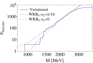
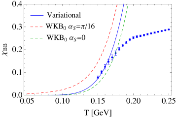
Figure 13: Cumulative number for the spectrum of baryons with the quark-diquark model (left panel) and baryonic $\chi_{BB}$ susceptibility obtained with that spectrum (right panel). We display as solid lines the result from the variational procedure of Sec. V.2, and as dashed lines the result from the WKB approximation at leading order. The points in the right panel are the lattice data of Ref. Bazavov et al. (2012). We have used the parameters in Eq. (42).

For completeness we provide some asymptotic results for finite quark and diquark mass corrections. For the cumulative number entering in the rhs of Eq. (58) one obtains

$$\Delta N_{0}(M)=-\frac{M^{4}(m_{q}^{2}+m_{D}^{2})}{48\pi\sigma^{3}}+\cdots\,,$$ (60)

for $m_{q}^{2}+m_{D}^{2}\ll M^{2}$. This translates into the following correction for the susceptibility on the rhs of Eq. (59)

$$\Delta\chi_{BB}(T)=-\frac{31\pi^{3}}{7560}(m_{q}^{2}+m_{D}^{2})\frac{T^{4}}{\sigma^{3}}+\cdots$$ (61)

for $m_{q}^{2}+m_{D}^{2}\ll T^{2}$.

More interesting is the behavior of the cumulative number when $M$ is near and above the (classical) threshold $M_{\rm threshold}=m_{q}+m_{D}$:

$$N_{0}(M)=\frac{64\sqrt{2}}{945\pi\sigma^{3}}\left(\frac{m_{q}m_{D}}{m_{q}+m_{D}}\right)^{3/2}(M-m_{q}-m_{D})^{9/2}+\cdots\,.$$ (62)

This region dominates the behavior of the susceptibility at small temperatures, namely:

$$\chi_{BB}(T)=\frac{(m_{q}m_{D})^{3/2}T^{3}}{\pi^{2}\sigma^{3}}e^{-(m_{q}+m_{D})/T}+\cdots$$ (63)

for $T\ll m_{q}+m_{D}$. This temperature region is appropriate for the values of $m_{q}$, $m_{D}$ and $T$ considered in this work.

Appendix B Sign of the cross susceptibility for degenerate flavors in QCD

In this Appendix we present a proof of the inequality in (18). The arguments hold in presence of a lattice regulator. We assume three flavors, $a=u,d,s$ with $u$ and $d$ degenerated. The partition function is

$$\begin{split}Z&=\int{\mathcal{D}}U\prod_{a}{\mathcal{D}}\bar{\psi}_{a}{\mathcal{D}}\psi_{a}\,e^{-S_{g}(U)-\sum_{a}\bar{\psi}_{a}D_{a}(U)\psi_{a}}\\ &=\int{\mathcal{D}}U\,e^{-S_{g}(U)}\prod_{a}\det D_{a}(U).\end{split}$$ (64)

$S_{g}(U)$ is the Euclidean gluonic action and (for simplicity here we use a notation of QCD in the continuous formulation),

$$D_{a}(U)=\gamma_{\mu}(\partial_{\mu}+iA_{\mu})+m_{a}\,,$$ (65)

where the gluon field $A_{\mu}(x)$ is a Hermitian matrix and $m_{a}$ is the mass of the flavor $a$. The Dirac matrices are Hermitian.

As is well known Montvay and Munster (1997), the identity

$$\gamma_{5}D_{a}(U)\gamma_{5}=D_{a}(U)^{\dagger}$$ (66)

implies that the eigenvalues of the Dirac operator are either real or come in conjugated pairs, hence $\det D_{a}(U)$ is real. Because $u$ and $d$ are degenerated, the weight $\det D_{u}(U)\det D_{d}(U)$ is positive. The weight $\det D_{s}(U)$ will be assumed to be positive too as required to be able to apply importance sampling Monte Carlo with dynamical quarks. This allows to define the real action

$$S_{q}(U)=-\sum_{a}\log\det D_{a}(U),$$ (67)

so that

$$Z=\int{\mathcal{D}}U\,e^{-S_{g}(U)-S_{q}(U)}.$$ (68)

The operator counting the flavor $a$ is

$$Q_{a}=\int d^{3}x\,\bar{\psi}_{a}(x)\gamma_{0}\psi_{a}(x)\quad a=u,d,s.$$ (69)

Because this quantity is conserved, we can use equivalently

$$Q_{a}=T\int d^{4}x\,\bar{\psi}_{a}(x)\gamma_{0}\psi_{a}(x)$$ (70)

where $T=1/\beta$ is the temperature. Its expectation value can be obtained using Wick’s theorem

$$\langle Q_{a}\rangle=\frac{T}{Z}\int{\mathcal{D}}Ue^{-S_{g}(U)-S_{q}(U)}(-1){\rm Tr}(\gamma_{0}D_{a}^{-1}(U)).$$ (71)

Of course this expectation value vanishes due to charge conjugation. Namely, using $D_{a}(U^{c})=CD_{a}(U)^{T}C^{-1}$ with $U^{c}\equiv U^{*}$ (or $A_{\mu}^{c}=-A_{\mu}^{T}$), and $C\gamma_{\mu}^{T}C^{-1}=-\gamma_{\mu}$, it follows that the measure including the actions are even under $U\to U^{c}$, whereas ${\rm Tr}(\gamma_{0}D_{a}^{-1}(U))$ is odd.

For the $ud$ correlation, again applying Wick contractions,

$$\langle\Delta Q_{u}\Delta Q_{d}\rangle=\frac{T^{2}}{Z}\int{\mathcal{D}}Ue^{-S_{g}(U)-S_{q}(U)}{\rm Tr}(\gamma_{0}D_{u}^{-1}(U))^{2}.$$ (72)

This quantity is negative definite because ${\rm Tr}(\gamma_{0}D_{a}^{-1}(U))$ is purely imaginary, as follows from

$$(\gamma_{0}D_{a}(U))^{\dagger}=-(\gamma_{5}\gamma_{0})\gamma_{0}D_{a}(U)(\gamma_{5}\gamma_{0})^{-1}.$$ (73)

One observation is that the fact that ${\rm Tr}(\gamma_{0}D_{a}^{-1}(U))$ is purely imaginary provides another proof of $\langle Q_{a}\rangle=0$ since this quantity is real, because $Q_{a}$ is Hermitian in the real time formulation.

Another observation is that $\chi_{ud}\leq 0$ will always hold in a Monte Carlo calculation, since ${\rm Tr}(\gamma_{0}D_{a}^{-1}(U))^{2}\leq 0$ for every configuration, even if the assumption $\det D_{s}(U)>0$ were violated. On the other hand, for $\langle Q_{u}^{2}\rangle$ there are two Wick contractions

$$\begin{split}\langle(\Delta Q_{u})^{2}\rangle&=\frac{T^{2}}{Z}\int{\mathcal{D}}Ue^{-S_{g}(U)-S_{q}(U)}\Big{(}{\rm Tr}(\gamma_{0}D_{u}^{-1}(U))^{2}\\ &\quad-{\rm Tr}(\gamma_{0}D_{u}^{-1}(U)\gamma_{0}D_{u}^{-1}(U))\Big{)}.\end{split}$$ (74)

Eq. (73) again implies that the second term is real and the inequality $\chi_{uu}\geq|\chi_{ud}|$ implies that this second term is not only positive but at least twice as large (in average) as minus the first one. Since there is no reason to expect that ${\rm Tr}(\gamma_{0}D_{u}^{-1}(U))^{2}-{\rm Tr}(\gamma_{0}D_{u}^{-1}(U)\gamma_{0}D_{u}^{-1}(U))$ is definite positive for each gauge configuration, the condition $\chi_{uu}\geq|\chi_{ud}|$ could fail to hold for nonpositive definite $\det D_{s}(U)$, thereby providing a test on this.

References

- Patrignani et al. (2016) C. Patrignani et al. (Particle Data Group), Chin. Phys. C40, 100001 (2016).
- Bohm and Sato (2005) A. R. Bohm and Y. Sato, Phys. Rev. D71, 085018 (2005), arXiv:hep-ph/0412106 [hep-ph] .
- Hagedorn (1965) R. Hagedorn, Nuovo Cim. Suppl. 3, 147 (1965).
- Hagedorn (1985) R. Hagedorn, Melting Hadrons, Boiling Quarks - From Hagedorn Temperature to Ultra-Relativistic Heavy-Ion Collisions at CERN: With a Tribute to Rolf Hagedorn, Lect. Notes Phys. 221, 53 (1985), [,287(2016)].
- Borsanyi et al. (2014) S. Borsanyi, Z. Fodor, C. Hoelbling, S. D. Katz, S. Krieg, and K. K. Szabo, Phys. Lett. B730, 99 (2014), arXiv:1309.5258 [hep-lat] .
- Bazavov et al. (2014) A. Bazavov et al. (HotQCD), Phys. Rev. D90, 094503 (2014), arXiv:1407.6387 [hep-lat] .
- Ruiz Arriola et al. (2014) E. Ruiz Arriola, L. L. Salcedo, and E. Megias, 54th Cracow School of Theoretical Physics: QCD meets experiment, Acta Phys. Polon. B45, 2407 (2014), arXiv:1410.3869 [hep-ph] .
- Godfrey and Isgur (1985) S. Godfrey and N. Isgur, Phys. Rev. D32, 189 (1985).
- Capstick and Isgur (1986) S. Capstick and N. Isgur, Proceedings, International Conference on Hadron Spectroscopy: College Park, Maryland, April 20-22, 1985, Phys. Rev. D34, 2809 (1986).
- Ruiz Arriola et al. (2012) E. Ruiz Arriola, W. Broniowski, and P. Masjuan, Proceedings, Conference on Modern approaches to nonperturbative gauge theories and their applications (Light Cone 2012): Cracow, Poland, July 8-13, 2012, (2012), 10.5506/APhysPolBSupp.6.95, [Acta Phys. Polon. Supp.6,95(2013)], arXiv:1210.7153 [hep-ph] .
- Broniowski (2016) W. Broniowski, Proceedings, Mini-Wokshop Bled 2016: Quarks, Hdrons, Matter: Bled, Slovenia, July 3-10, 2016, Bled Workshops Phys. 17, 1 (2016), arXiv:1610.09676 [nucl-th] .
- Borsanyi et al. (2012) S. Borsanyi, Z. Fodor, S. D. Katz, S. Krieg, C. Ratti, and K. Szabo, JHEP 01, 138 (2012), arXiv:1112.4416 [hep-lat] .
- Bazavov et al. (2012) A. Bazavov et al. (HotQCD), Phys. Rev. D86, 034509 (2012), arXiv:1203.0784 [hep-lat] .
- Ruiz Arriola et al. (2016) E. Ruiz Arriola, W. Broniowski, E. Megias, and L. L. Salcedo, in Workshop on Excited Hyperons in QCD Thermodynamics at Freeze-Out (YSTAR2016) Mini-Proceedings (2016) pp. 128–139, arXiv:1612.07091 [hep-ph] .
- Capstick (1992) S. Capstick, Phys. Rev. D46, 2864 (1992).
- Hey and Kelly (1983) A. J. G. Hey and R. L. Kelly, Phys. Rept. 96, 71 (1983).
- Capstick and Roberts (2000) S. Capstick and W. Roberts, Prog. Part. Nucl. Phys. 45, S241 (2000), arXiv:nucl-th/0008028 [nucl-th] .
- Anselmino et al. (1993) M. Anselmino, E. Predazzi, S. Ekelin, S. Fredriksson, and D. B. Lichtenberg, Rev. Mod. Phys. 65, 1199 (1993).
- Klempt et al. (2017) E. Klempt, A. V. Sarantsev, and U. Thoma, Proceedings, SFB/TRR16 Symposium: Subnuclear Structure of Matter: Achievements and Challenges: Bonn, Germany, June 6-9, 2016, EPJ Web Conf. 134, 02002 (2017).
- Fleck et al. (1988) S. Fleck, B. Silvestre-Brac, and J. M. Richard, Phys. Rev. D38, 1519 (1988).
- Santopinto (2005) E. Santopinto, Phys. Rev. C72, 022201 (2005).
- Ferretti et al. (2011) J. Ferretti, A. Vassallo, and E. Santopinto, Phys. Rev. C83, 065204 (2011).
- Gutierrez and De Sanctis (2014) C. Gutierrez and M. De Sanctis, Eur. Phys. J. A50, 169 (2014).
- Alexandrou et al. (2006) C. Alexandrou, P. de Forcrand, and B. Lucini, Phys. Rev. Lett. 97, 222002 (2006), arXiv:hep-lat/0609004 [hep-lat] .
- DeGrand et al. (2008) T. DeGrand, Z. Liu, and S. Schaefer, Phys. Rev. D77, 034505 (2008), arXiv:0712.0254 [hep-ph] .
- Eichmann et al. (2016) G. Eichmann, C. S. Fischer, and H. Sanchis-Alepuz, Phys. Rev. D94, 094033 (2016), arXiv:1607.05748 [hep-ph] .
- Ebert et al. (2011) D. Ebert, R. N. Faustov, and V. O. Galkin, Phys. Rev. D84, 014025 (2011).
- Masjuan and Ruiz Arriola (2017) P. Masjuan and E. Ruiz Arriola, Phys. Rev. D96, 054006 (2017), arXiv:1707.05650 [hep-ph] .
- Ruiz Arriola et al. (2017) E. Ruiz Arriola, P. Masjuan, and W. Broniowski, Proceedings, 9th Workshop ”Excited QCD” 2017: Sintra, Portugal, May 7-13, 2017, Acta Phys. Polon. Supp. 10, 1079 (2017), arXiv:1707.07508 [hep-ph] .
- Tanabashi et al. (2018) M. Tanabashi et al. (ParticleDataGroup), Phys. Rev. D98, 030001 (2018).
- Broniowski and Florkowski (2000) W. Broniowski and W. Florkowski, Phys. Lett. B490, 223 (2000), arXiv:hep-ph/0004104 [hep-ph] .
- Broniowski et al. (2004) W. Broniowski, W. Florkowski, and L. Ya. Glozman, Phys. Rev. D70, 117503 (2004), arXiv:hep-ph/0407290 [hep-ph] .
- Briceno et al. (2016) R. A. Briceno et al., Chin. Phys. C40, 042001 (2016), arXiv:1511.06779 [hep-ph] .
- Edwards et al. (2013) R. G. Edwards, N. Mathur, D. G. Richards, and S. J. Wallace (Hadron Spectrum), Phys. Rev. D87, 054506 (2013), arXiv:1212.5236 [hep-ph] .
- Osterwalder and Seiler (1978) K. Osterwalder and E. Seiler, Salerno Soliton Wkshp.1977:0201, Annals Phys. 110, 440 (1978).
- Tawfik (2005) A. Tawfik, Phys.Rev. D71, 054502 (2005).
- Caro et al. (1996) J. Caro, E. Ruiz Arriola, and L. Salcedo, J.Phys. G22, 981 (1996), arXiv:nucl-th/9410025 [nucl-th] .
- Bellwied et al. (2015) R. Bellwied, S. Borsanyi, Z. Fodor, S. D. Katz, A. Pasztor, C. Ratti, and K. K. Szabo, Phys. Rev. D92, 114505 (2015), arXiv:1507.04627 [hep-lat] .
- Asakawa and Kitazawa (2016) M. Asakawa and M. Kitazawa, Prog. Part. Nucl. Phys. 90, 299 (2016), arXiv:1512.05038 [nucl-th] .
- Bakry et al. (2015) A. S. Bakry, X. Chen, and P.-M. Zhang, Phys. Rev. D91, 114506 (2015), arXiv:1412.3568 [hep-lat] .
- Bissey et al. (2009) F. Bissey, A. I. Signal, and D. B. Leinweber, Phys. Rev. D80, 114506 (2009), arXiv:0910.0958 [hep-lat] .
- Bakry et al. (2018) A. Bakry, X. Chen, M. Deliyergiyev, A. Galal, S. Xu, and P. M. Zhang, Proceedings, 17th International Conference on Hadron Spectroscopy and Structure (Hadron 2017): Salamanca, Spain, September 25-29, 2017, PoS Hadron2017, 211 (2018), arXiv:1712.03109 [hep-lat] .
- Koma and Koma (2017) Y. Koma and M. Koma, Phys. Rev. D95, 094513 (2017), arXiv:1703.06247 [hep-lat] .
- Megias et al. (2014) E. Megias, E. Ruiz Arriola, and L. L. Salcedo, Phys. Rev. D89, 076006 (2014).
- Santopinto and Ferretti (2015) E. Santopinto and J. Ferretti, Phys. Rev. C92, 025202 (2015), arXiv:1412.7571 [nucl-th] .
- Luscher (1981) M. Luscher, Nucl. Phys. B180, 317 (1981).
- Jaffe (2005) R. L. Jaffe, Proceedings, 6th International Conference on Hyperons, charm and beauty hadrons (BEACH 2004): Chicago, USA, June 27-July 3, 2004, Phys. Rept. 409, 1 (2005), [,191(2004)], arXiv:hep-ph/0409065 [hep-ph] .
- Ruiz Arriola et al. (2018) E. Ruiz Arriola, J. E. Amaro, and R. Navarro Pérez, Proceedings, 17th International Conference on Hadron Spectroscopy and Structure (Hadron 2017): Salamanca, Spain, September 25-29, 2017, PoS Hadron2017, 134 (2018), arXiv:1711.11338 [nucl-th] .
- De Sanctis et al. (2016) M. De Sanctis, J. Ferretti, E. Santopinto, and A. Vassallo, Eur. Phys. J. A52, 121 (2016).
- Ruiz Arriola and Broniowski (2007) E. Ruiz Arriola and W. Broniowski, Quarks and nuclear physics. Proceedings, 4th International Conference, QNP 2006, Madrid, Spain, June 5-10, 2006, Eur. Phys. J. A31, 739 (2007), arXiv:hep-ph/0609266 [hep-ph] .
- Borsanyi et al. (2018) S. Borsanyi, Z. Fodor, J. N. Guenther, S. K. Katz, K. K. Szabo, A. Pasztor, I. Portillo, and C. Ratti, JHEP 10, 205 (2018), arXiv:1805.04445 [hep-lat] .
- Montvay and Munster (1997) I. Montvay and G. Munster, Quantum fields on a lattice, Cambridge Monographs on Mathematical Physics (Cambridge University Press, 1997).