The Quantum Hall ferroelectric helix in bilayer graphene

Abstract

We re-examine the nature of the ground states of bilayer graphene at odd integer filling factors within a simplified model of nearly degenerate $n=0$ and $n=1$ Landau levels. Previous Hartree-Fock studies have found that ferroelectric states with orbital coherence can be stabilized by tuning the orbital splitting between these levels. These studies indicated that, in addition to a uniform ferroelectric state, a helical ferroelectric phase with spontaneously broken translational symmetry is possible. By performing exact diagonalization on the torus, we argue that the system does not have a uniform coherent state but instead transitions directly from the uniform incoherent state into the ferroelectric helical phase. We argue that there is a realistic prospect to stabilize the helical ferroelectric state in bilayer graphene by tuning the interlayer electric field in a model that includes all single particle corrections to its zero energy eight-fold multiplet of Landau levels.

I Introduction

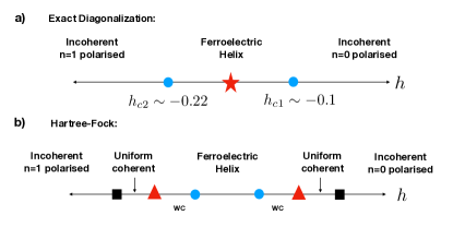
Figure 1: Summary of the phases observed in the orbitally mixed $n=0/1$ as a function of the orbital single particle splitting $h$. (a) The exact diagonalization results of the current study indicate the presence of only two phases: an incoherent adiabatically connected to the maximally polarized states, and a ferroelectric helical state. The red star indicates the orbital bias at which particle hole symmetry is achieved for which the system has equal population of the $n=0/1$ orbitals. (b) The Hartree-Fock studies find two other phases: the uniform orbitally coherent ferroelectric and a Wigner crystal (WC), see e.g. Ref .(Cote11, ) for a detailed estimate of the boundaries.

The last two decades have witnessed a rapid and formidable increase in the richness of the quantum Hall physics of monolayer and bilayer graphene Novoselov05 ; Novoselov06 ; Du09 ; Bolotin09 ; Dean11 ; Feldman12 ; Smet12 ; Young12 ; CastroNeto09 ; Abanin09 ; Abanin13 ; Toke07 ; Ki13 ; Papic11-1 ; Papic11-2 . In particular, bilayer graphene (BLG) possesses a unique zeroth Landau level manifold which features two nearly degenerate cyclotron orbital degrees of freedom with $n=0$ and $n=1$ character McCann06 , in addition to the two spins and two valleys making up a manifold with a total of eight levels. The interplay of strong Coulomb interactions, that stabilize integer quantum Hall states via quantum Hall ferromagnetism YSM , and the single particle splitting terms, can lead to an intricate variety of coherent states in this system Barlas08 ; Barlas10 ; Cote10 ; Cote11 ; Lambert ; Knothe . A notoriously interesting possibility, pointed out in Ref. Barlas08, , is the coherence between the states with different orbital character $n=0/n=1$. This coherence breaks spontaneously the real space inversion symmetry, resulting in the formation of a type of quantum Hall ferroelectric state, which is expected to have a linearly dispersing Goldstone mode (this form of quantum Hall ferroelectric state is distinct from that proposed in Ref. Zheng, which results from spontaneous valley polarization). Following these initial studies, it was later argued based on Hartree-Fock theory Cote11 , that an analogue of Dzyaloshinskii-Moriya interaction allowed by the breaking of inversion symmetry, can drive the softening of this Goldstone mode at a finite wave-vector, leading to the formation of ferroelectric helical state. The phase diagram as a function of the single-particle splitting of the $n=0/n=1$ orbitals obtained from Hartree-Fock is depicted in Fig.1(b), which additionally features a Wigner crystal state.

To this date there are very few studies incorporating correlation effects beyond Hartree-Fock on this problem. One exact diagonalization study AbaninPapic restricted itself to the case of zero single particle splitting between $n=0$ and $n=1$ orbitals, and found that in such case the ground state is a trivial integer quantum Hall state adiabatically connected to the fully polarized state into the $n=0$ orbital with a full gap to all excitations. As we will see, however the interesting ferroelectric states predicted by Hartree-Fock theory tend to occur at negative splitting when the $n=1$ orbital is energetically favored, explaining why they were not observed in Ref. (AbaninPapic, ).

In this paper we concentrate on phases with full spin and valley polarization and just keep the two orbital degrees of freedom $n=0$ and $n=1$, and restrict to total filling factor $\nu=1$. Using the torus geometry we diagonalize exactly the Hamiltonian for up to 14 electrons, which allows us to obtain information on ground states and some of the low-lying excited states. We pay special attention to the role of a nontrivial particle-hole symmetry, identified in Ref. (Shizuya12, ), which maps states with filling $\nu$ onto states with $2-\nu$ in the two orbital manifold. Remarkably, this symmetry acts non-trivially on the bare single particle-splitting between the $n=0$ and $n=1$ orbitals, and for a Hamiltonian to be particle-hole invariant under this symmetry it must have a negative splitting favoring the $n=1$ orbital.

We will show that the simple polarized incoherent phase observed in Ref.(AbaninPapic, ) can be captured by perturbation theory and show that its excited states can be reproduced by time-dependent Hartree-Fock theory. We also find that for some range of orbital splitting there is evidence for a phase with broken translation symmetry that we identify as the helical ferroelectric phase seen in HF calculations. However, we find no evidence for a spatially uniform orbitally coherent state, because we do not observe any translationally invariant phase with its characteristic Goldstone mode. We depict the approximate phase diagram resulting from our study in Fig.1(a). We will also show that there is a realistic prospect to realise the ferroelectric helical state in BLG. Recent experiments have achieved a detailed understanding and a remarkable degree of control over the single particle splittings in the zeroth Landau level manifold of BLG Hunt ; Andrea2017 ; Dean . Because the valley degree of freedom is locked to the layer index in the zeroth Landau level of BLG, this degree of freedom can be easily controlled by applying an interlayer bias. The spin splitting on the other hand can be controlled with in-plane fields. It is therefore, possible to achieve the conditions in which the system is valley and spin polarized and the relevant active degrees of freedom are the $n=0$ and $n=1$ orbitals. The splitting between the $n=0$ and $n=1$ levels is intimately related to hopping terms that break particle-hole invariance in bilayer graphene Jeil . We will also show, however, that there is a way to experimentally control the splitting between the $n=0$ and $n=1$ orbitals by tuning the interlayer bias to sufficiently large values.

Our paper is organized as follows, in section II we discuss the realistic band structure of BLG and show that the level crossing between $n=0/n=1$ lies within a realistic range of parameters. In section III we explain the peculiar particle-hole symmetry of the model obtained by assuming full spin and valley polarization. Section IV contains some definitions of finite-size torus wavefunctions. Section V summarize the Hartree-Fock treatment. In section VI we give results of exact diagonalization studies. Section VII is devoted to the incoherent phase and its excitations. Section VIII contains our findings about the broken translation symmetry phase. Our conclusions are presented in section IX.

II Band structure of bilayer graphene

The four band model containing all leading corrections to bilayer graphene’s Hamiltonian for a single spin and valley in the presence of a magnetic field has the form Jeil  :

$$H_{4b}=\omega_{0}\left(\begin{array}[]{cccc}\frac{u}{2\omega_{0}}&a^{\dagger}&-\frac{\gamma_{4}}{\gamma_{0}}a^{\dagger}&-\frac{\gamma_{3}}{\gamma_{0}}a\\ a&\frac{\Delta^{\prime}+u}{2\omega_{0}}&\frac{\gamma_{1}}{\omega_{0}}&-\frac{\gamma_{4}}{\gamma_{0}}a^{\dagger}\\ -\frac{\gamma_{4}}{\gamma_{0}}a&\frac{\gamma_{1}}{\omega_{0}}&\frac{\Delta^{\prime}-u}{2\omega_{0}}&a^{\dagger}\\ -\frac{\gamma_{3}}{\gamma_{0}}a^{\dagger}&-\frac{\gamma_{4}}{\gamma_{0}}a&a&-\frac{u}{2\omega_{0}}\\ \end{array}\right).$$ (1)

Here $\omega_{0}=\sqrt{2}v_{0}/\ell\approx 30.6{\rm meV}\sqrt{{\rm B[T]}}$, with the magnetic length $\ell=\sqrt{\hbar c/eB}$, $\gamma_{0}\approx 2.61$eV, $\gamma_{1}\approx 361$meV, $\gamma_{3}\approx 283$meV, $\gamma_{4}\approx 138$meV, $\Delta^{\prime}\approx 15$meV, and $u$ is the energy difference between top and bottom layers controlled by a perpendicular electric field. This Hamiltonian has been successfully employed in detailed modeling of Landau levels for integer Hunt and fractional quantum Hall states recently Andrea2017 .

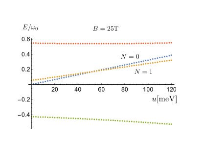
Figure 2: Landau levels for a single spin-valley in BLG as a function of interlayer bias. The bias can tune a level crossing between $n=0$ and $n=1$. There is a sizable energy separation from higher Landau levels throughout justifying the projection into the two $n=0$ and $n=1$ LLs.

In this Hamiltonian the terms $\Delta^{\prime}$ and $\gamma_{4}$ break particle-hole symmetry and induce a splitting between the $n=0$ and $n=1$ LLs at zero interlayer bias $u$ which favors $n=0$. This renders the ground state trivially polarized into $n=0$ at $u=0$, and therefore under normal conditions one would not expect the physics that we will describe in this paper to appear. However, as illustrated in Fig. 2, the interlayer bias can be used to control the splitting between these levels and successfully induce a level crossing making the $n=1$ lower in energy as we desire. The value required to achieve this crossing is independent of the magnetic field and, neglecting the trigonal warping term ($\gamma_{3}\rightarrow 0$), can be estimated to be :

$$u_{0}=\frac{2\gamma_{4}\gamma_{1}}{\gamma_{0}}+\Delta^{\prime}\left(1+\left(\frac{\gamma_{4}}{\gamma_{0}}\right)^{2}\right)\approx 53.2{\rm meV}.$$ (2)

which should be within experimental reach. In Fig. 3 we show this value as green dots (including the trigonal warping term). At this value one expects the boundary between the state fully polarized into $n=0$ and the coherent states. The orange dots are the required values in order to overcome the splitting produced by the exchange interactions with the vacuum (analogous to the well-known Lamb shift in atomic physics)Shizuya12 for bare Coulomb interactions so that the system has approximate particle-hole symmetry. The blue dots depict the expected Hartree-Fock boundary between coherent and fully $n=1$ polarized states Cote11 . Taking bare Coulomb interactions, these two boundaries correspond to the single particle energy splitting given respectively by:

$$E_{1}-E_{0}=\epsilon_{\mathrm{Lamb}} = \frac{e^{2}}{\epsilon\ell}\frac{1}{16}\sqrt{\frac{\pi}{2}},$$

$$E_{1}-E_{0}=\epsilon_{\mathrm{orb.pol.}} = \frac{e^{2}}{\epsilon\ell}\frac{1}{8}\sqrt{\frac{\pi}{2}}.$$

Finally, in Fig. 4 we illustrate the overlaps of the LL levels in the full four-band model with the idealized two-band model as a function of the interlayer bias and field. We see an excellent overlap for $n=0$ and a good overlap for $n=1$. The latter is known to decrease as the magnetic field increases Andrea2017 , but as we see there is no substantial change as a function of interlayer bias.

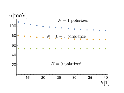
Figure 3: Expected schematic phase diagram as a function of interlayer bias $u$ and perpendicular magnetic field. Identification of phases come Hartree-Fock calculations. The green dots are where the bare single particle energies of $n=0$ and $n=1$ become degenerate. The yellow dots lie where approximate particle symmetry is expected in the presence of Coulomb interactions and the blue dots are the expected location at which the system polarizes into $n=1$. We assume that the bilayer graphene sample is on top of a hexagonal boron nitride substrate with screening constant $\epsilon\approx 6.6$ as in ref.(Andrea2017, ).

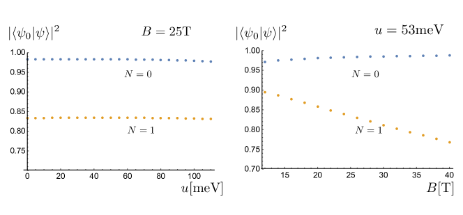
Figure 4: Overlaps between the ideal two-band model Landau level wavefunctions and the four-band model wavefunctions as a function of interlayer bias and magnetic field.

III Particle-hole symmetry between $n=0$ and $n=1$ Landau levels

Consider the two-band model of bilayer graphene :

$$\mathcal{H}_{K}=\left(\matrix{0&-(\Pi_{x}-i\Pi_{y})^{2}/2m^{*}\cr-(\Pi_{x}+i\Pi_{y})^{2}/2m^{*}&0}\right)$$ (3)

where $m^{*}$ is an effective mass and $\Pi_{x,y}=p_{x,y}+eA_{x,y}/c$. This is the Hamiltonian concerning valley $K$ and spin is polarized. The single-particle spectrum has then two zero-energy states :

$$E_{0K}=E_{1K}=0$$ (4)

and the remainder of the spectrum depends upon the magnetic field :

$$E_{nK}=\mathrm{sign}(n)\omega_{c}\sqrt{|n|(|n|-1)},\quad|n|\geq 2,$$ (5)

where $n$ is an integer positive or negative and $\omega_{c}=eB/m^{*}$. The corresponding eigenstates are given by :

$$\Phi_{n}=\left(\matrix{\phi_{n}\cr 0}\right),\quad n=0,1$$ (6)

$$\Phi_{n}=\frac{1}{\sqrt{2}}\left(\matrix{\phi_{|n|}\cr\phi_{|n|-2}}\right),\quad n\leq-2,\quad\Phi_{n}=\frac{1}{\sqrt{2}}\left(\matrix{-\phi_{|n|}\cr\phi_{|n|-2}}\right),\quad n\geq+2,$$ (7)

where $\phi_{n}$ are standard cyclotron eigenstates for particles with parabolic dispersion relation. We now consider two-body interactions written in second quantization :

$$\mathcal{V}=\frac{1}{2}\sum_{1234}V_{1234}\,\,c^{\dagger}_{n_{1},j_{1}}c^{\dagger}_{n_{2},j_{2}}c_{n_{3},j_{3}}c_{n_{4},j_{4}}$$ (8)

with Landau level indices $n_{i}=0,1$ and guiding center coordinates $j_{i}$ and the big indices $\{1234\}$ are a short-hand for the combined indices. We now use the particle-hole conjugation operator $\mathcal{C}$ which is defined by :

$$\mathcal{C}^{\dagger}c^{\dagger}_{nj}\mathcal{C}=c_{nj}.$$ (9)

When acting on Eq.(8) we find :

$$\mathcal{C}^{\dagger}\mathcal{V}\mathcal{C}=\mathcal{V}+\sum_{12M}c^{\dagger}_{1}c_{2}(V_{1M2M}+V_{M2M1}-V_{2MM1}-V_{M21M})+{\rm const}$$ (10)

The particle-hole transformation generates an additional one-body term which can written as  :

$$\Delta_{0}\sum_{m}c^{\dagger}_{0m}c_{0m}+\Delta_{1}\sum_{m}c^{\dagger}_{1m}c_{1m},$$ (11)

The constants $\Delta_{0,1}$ are geometry-dependent and they are distinct $\Delta_{0}\neq\Delta_{1}$. So even if we start with exactly degenerate $n=0$ and $n=1$ LLs the particle-hole symmetry leads to a nontrivial splitting between them. If we now focus on the state with total filling factor $\nu=1$ then the particle-symmetry above implies that the full spectrum of the Hamiltonian Eq.(8) should be the same after addition of the one-body splitting Eq.(11).

IV Torus definitions

We consider a torus that is obtained by periodic boundary conditions applied to a rectangular domain spanned by vectors $\mathbf{L}_{1}=L_{x}\mathbf{\hat{x}}$ and $\mathbf{L}_{2}=L_{y}\mathbf{\hat{y}}$. The aspect ratio is defined as :

$$\mathrm{AR}=\frac{L_{x}}{L_{y}}.$$ (12)

Periodic boundary conditions are imposed by magnetic translations Zak64 $t(\mathbf{L})=\exp\left(\frac{i}{\hbar}\mathbf{L}\cdot\Pi-i\frac{\mathbf{\hat{z}}\cdot(\mathbf{L}\times\mathbf{r})}{\ell^{2}}\right)$. Using the Landau gauge $\mathbf{A}=Bx\mathbf{\hat{y}}$ for in this study, these act as $t(\mathbf{L})\psi(\mathbf{r})=\exp(\frac{iy\mathbf{\hat{x}}\cdot\mathbf{L}}{\ell^{2}})\psi(\mathbf{r}+\mathbf{L})$. The boundary conditions read $t(\mathbf{L}_{1,2})\psi(\mathbf{r})=\psi(\mathbf{r})$. The two conditions are compatible only if the rectangle is pierced by an integral number of flux quanta :

$$N_{\phi}=\frac{\left|\mathbf{L}_{1}\times\mathbf{L}_{2}\right|}{2\pi\ell^{2}}=\frac{L_{x}L_{y}}{2\pi\ell^{2}}.$$ (13)

The $n=0$ states can be written as Haidekker18  :

$$\eta_{0m}(z)=\frac{1}{\sqrt{\ell L_{2}\sqrt{\pi}}}\vartheta\left[\begin{array}[]{c}m/N_{\phi}\\ 0\end{array}\right]\left(\frac{i\pi N_{\phi}z}{L_{2}}\Big{|}N_{\phi}i\right)e^{-\frac{x^{2}}{2\ell^{2}}},$$ (14)

where $m=0,1,\dots,(N_{\phi}-1)$, $z=x+iy$, and we have used Jacobi elliptic functions with characteristics Mumford87  :

$$\vartheta\left[\begin{array}[]{c}a\\ b\end{array}\right](z|\tau)=\sum_{n=-\infty}^{\infty}e^{i\pi\tau(n+a)^{2}+2i(n+a)(z+b\pi)}.$$ (15)

Higher Landau orbitals are obtained using the LL raising operator, which in our gauge takes the form : $\hat{a}^{\dagger}=\frac{\ell}{\sqrt{2}}\left(i\partial_{x}+\partial_{y}-\frac{ix}{\ell^{2}}\right)=\frac{\ell}{\sqrt{2}}\left(2i\partial_{z}-\frac{ix}{\ell^{2}}\right)$. Thus we have :

$$\eta_{n,j}(z) = \frac{(\hat{a}^{\dagger})^{n}}{\sqrt{n!}}\eta_{n0}(z)=$$

$$= \frac{1}{(L_{y}\sqrt{\pi})^{1/2}}\sum_{k}H_{n}\left(\frac{x}{\ell}-\frac{kL_{x}}{\ell}-\frac{2\pi j\ell}{L_{y}}\right)\exp\left(-i\left(\frac{kL_{x}}{\ell^{2}}+\frac{2\pi j}{L_{y}}\right)y-\frac{1}{2\ell^{2}}\left(x-kL_{x}-\frac{2\pi j\ell^{2}}{L_{y}}\right)^{2}\right),$$

where $H_{n}$ is a a Hermite polynomial. We note that $\eta_{nm}(z)$ is normalized for the principal domain of the torus :

$$\int_{0}^{L_{y}}dy\int_{0}^{L_{x}}dx\eta^{\ast}_{n^{\prime}m^{\prime}}(x+iy)\eta_{nm}(x+iy)=\delta_{nn^{\prime}}\delta_{mm^{\prime}}.$$ (17)

V Hartree-Fock treatment

The difference of the spatial profile of the $n=0$ and $n=1$ Landau states allows for nontrivial electric dipole structures when both of these states are relevant to the ordering in a partially filled Landau band. Côté, Fouquet and Luo Cote11 have elaborated the Hartree-Fock mean-field theory for such systems. Treating the energy splitting $h$ between the $n=1$ and the $n=0$ orbitals as a parameter, the mean-field energy per particle reads, in units of $e^{2}/(\epsilon\ell)$ and having the thermodynamic limit in mind, as :

$$\frac{E_{\textrm{\scriptsize HF}}}{N} = -\frac{11}{32}\sqrt{\frac{\pi}{2}}-h\left\langle\rho_{z}(\mathbf{q}=0)\right\rangle$$

$$+\frac{1}{2}\sum_{\mathbf{q}}a(q)\left(\left\langle\rho_{x}(-\mathbf{q})\right\rangle\left\langle\rho_{x}(\mathbf{q})\right\rangle+\left\langle\rho_{y}(-\mathbf{q})\right\rangle\left\langle\rho_{y}(\mathbf{q})\right\rangle\right)+$$

$$+\frac{1}{2}\sum_{\mathbf{q}}b(q)\left(\begin{array}[]{cc}\left\langle\rho_{x}(-\mathbf{q})\right\rangle&\left\langle\rho_{y}(-\mathbf{q})\right\rangle\end{array}\right)\left(\begin{array}[]{cc}\cos(2\varphi_{q})&\sin(2\varphi_{q})\\ \sin(2\varphi_{q})&-\cos(2\varphi_{q})\end{array}\right)\left(\begin{array}[]{cc}\left\langle\rho_{x}(\mathbf{q})\right\rangle\\ \left\langle\rho_{y}(\mathbf{q})\right\rangle\end{array}\right)+$$

$$+\frac{1}{2}\sum_{\mathbf{q}}c(q)\left\langle\rho_{z}(-\mathbf{q})\right\rangle\left\langle\rho_{z}(\mathbf{q})\right\rangle+$$

$$+\frac{i}{4}\sum_{\mathbf{q}}d(q)(\mathbf{\hat{z}}\times\mathbf{\hat{q}})\cdot(\left\langle\vec{\rho}(-\mathbf{q})\right\rangle\times\left\langle\vec{\rho}(\mathbf{q})\right\rangle),$$

where the pseudospin density operator $\rho(\mathbf{q})$ is written as $\rho_{x}(\mathbf{q})=-(\rho_{1,0}(\mathbf{q})+\rho_{0,1}(\mathbf{q}))/2$, $\rho_{y}(\mathbf{q})=(\rho_{1,0}(\mathbf{q})-\rho_{0,1}(\mathbf{q}))/2i$, $\rho_{z}(\mathbf{q})=(\rho_{0,0}(\mathbf{q})-\rho_{1,1}(\mathbf{q}))/2$, with

$$\rho_{n,n^{\prime}}(\mathbf{q})=\frac{1}{N_{\phi}}\sum_{X}e^{-iq_{x}x+iq_{x}q_{y}\ell^{2}/2}c^{\dagger}_{nX}c_{n^{\prime},X-q_{y}\ell^{2}};$$ (25)

$\varphi_{q}$ is the angle of vector $\mathbf{q}$, and we have used real-valued functions that eventually follow from the matrix elements of the Coulomb interaction, defined in Ref. Cote11, , which can be written in closed form as

$$a(q) = q\ell e^{-q^{2}\ell^{2}/2}-\sqrt{\frac{\pi}{2}}\left(1+q^{2}\ell^{2}/2\right)e^{-q^{2}\ell^{2}/4}I_{1}\left(q^{2}\ell^{2}/4\right)-\sqrt{\frac{\pi}{8}}q^{2}\ell^{2}e^{-q^{2}\ell^{2}/4}I_{1}\left(q^{2}\ell^{2}/4\right),$$

$$b(q) = q\ell e^{-q^{2}\ell^{2}/2}-\sqrt{\frac{\pi}{8}}e^{-q^{2}\ell^{2}/4}I_{0}\left(q^{2}\ell^{2}/4\right)+\sqrt{\frac{\pi}{2}}\left(1+q^{2}\ell^{2}/2\right)e^{-q^{2}\ell^{2}/4}I_{1}\left(q^{2}\ell^{2}/4\right),$$

$$c(q) = \frac{q^{3}\ell^{3}}{4}e^{-q^{2}\ell^{2}/2}-\sqrt{2\pi}e^{-q^{2}\ell^{2}/4}\left(\frac{3}{8}+\frac{q^{2}\ell^{2}}{8}+\frac{q^{4}\ell^{4}}{16}\right)I_{0}\left(q^{2}\ell^{2}/4\right)+\sqrt{2\pi}e^{-q^{2}\ell^{2}/4}\left(\frac{q^{4}\ell^{4}}{16}-\frac{q^{2}\ell^{2}}{4}\right)I_{1}\left(q^{2}\ell^{2}/4\right),$$

$$d(q) = \sqrt{2}q^{2}\ell^{2}e^{-q^{2}\ell^{2}/2}+\sqrt{\frac{\pi}{32}}q^{3}\ell^{3}e^{-q^{2}\ell^{2}/4}I_{0}\left(q^{2}\ell^{2}/4\right)-\sqrt{\frac{\pi}{32}}q(3+q^{2}\ell^{2})\ell e^{-q^{2}\ell^{2}/4}I_{1}\left(q^{2}\ell^{2}/4\right).$$

Here, $h$ can be related to the interlayer bias $u$ but we prefer to handle it as a parameter throughout this study. The $a(q)$ and $c(q)$ terms are anisotropic exchange coupling between pseudospins, reminiscent of the XXZ model; the $b(q)$ term is basically the dipole-dipole electrostatic interaction; and the $d(q)$ term is a Dzyaloshinskii-Moriya type interaction between pseudospins. We emphasize that even though the above formulas refer to $N_{\phi}$ flux quanta, the $N_{\phi}\to\infty$ limit is implied; several assumptions in the analysis based on Eq. (V) are applicable only this case. In the phase diagram based on Eq. (V) the region around the particle-hole symmetric value of $h=0$ the system exhibits pseudospin helical state, while a uniform liquid is expected outside of this region. The latter uniform state may exhibit orbital phase coherence with the ensuing ferroelectric dipole ordering.

For a comparison with exact diagonalization, we consider the Hartree-Fock approximation on the torus. By standard mean-field decoupling of the interaction part of the Hamiltonian

$$\mathcal{H}_{\textrm{\scriptsize C}} = \frac{1}{2}\sum_{n_{1},n_{2},n_{3},n_{4}=0}\sum_{m_{1},m_{2},m_{3},m_{4}=0}^{N_{\phi}-1}\mathcal{A}_{m_{1},m_{2},m_{3},m_{4}}^{n_{1},n_{2},n_{3},n_{4}}:\rho_{n_{1}m_{1},n_{4}m_{4}}\rho_{n_{2}m_{2},n_{3}m_{3}}:,$$ (26)

$$\rho_{nm,n^{\prime}m^{\prime}} = c^{\dagger}_{nm}c_{n^{\prime}m^{\prime}},$$ (27)

where the matrix elements $\mathcal{A}_{m_{1},m_{2},m_{3},m_{4}}^{n_{1},n_{2},n_{3},n_{4}}$ among the basis states $\eta_{nm}$ are given in Eq. (31) below. The uniform state on the torus is the one where each guiding center position is occupied by the same linear combination of the $n=0,1$ orbitals :

$$\left|\Psi_{\textrm{\scriptsize U}}\right\rangle=\prod_{m=0}^{N_{\phi}-1}\left(\cos\left(\frac{\theta}{2}\right)e^{i\phi/2}c^{\dagger}_{0m}+\sin\left(\frac{\theta}{2}\right)e^{-i\phi/2}c^{\dagger}_{1m}\right)|0\rangle.$$ (28)

With the definition : $\rho^{x}_{mm^{\prime}}=(\left\langle\rho_{1m,0m^{\prime}}\right\rangle+\left\langle\rho_{0m,1m^{\prime}}\right\rangle)/2$, $\rho^{y}_{mm^{\prime}}=(\left\langle\rho_{1m,0m^{\prime}}\right\rangle-\left\langle\rho_{0m,1m^{\prime}}\right\rangle)/2i$, $\rho^{z}_{mm^{\prime}}=(\left\langle\rho_{0m,0m^{\prime}}\right\rangle-\left\langle\rho_{1m,1m^{\prime}}\right\rangle)/2$, this state corresponds to the dipole density :

$$\vec{\rho}_{mm^{\prime}}=\delta_{mm^{\prime}}\frac{1}{2}\left(\begin{array}[]{c}\sin\theta\cos\phi\\ \sin\theta\sin\phi\\ \cos\theta\end{array}\right).$$ (29)

By some algebra, we arrive at the energy expression :

$$\frac{E_{\textrm{\scriptsize HF}}}{N}=-\epsilon_{N}+\frac{h+H}{2}\cos\theta+A\sin^{2}\theta+C\cos^{2}\theta+B\sin^{2}\theta\cos(2\phi),$$ (30)

where $A,B,C,H$ are some constants and the energy $\epsilon_{N}$ has a lengthy expression that goes to $-\frac{11}{32}\sqrt{\frac{\pi}{2}}$ for large $N$. These quantities have the symmetry $A(\mathrm{AR})-C(\mathrm{AR})=A(1/\mathrm{AR})-C(1/\mathrm{AR})$, $B(\mathrm{AR})=-B(1/\mathrm{AR})$, and $H(\mathrm{AR})=H(1/\mathrm{AR})$. Hence $B$ vanishes for a square torus $\mathrm{AR}=1$, and we also have $B>0\iff\mathrm{AR}<1$. Thus, for $\mathrm{AR}>1$ we have $\phi={\pi}/{2}$, otherwise $\phi=0$; if $\mathrm{AR}\to{1}/{\mathrm{AR}}$, the preferential direction of the pseudospins rotate by ${\pi}/{2}$, and there is no preferential direction on the square torus. Numerical values for various $N_{\phi}$ are shown in Fig. 5. Clearly, the deviation from the infinite-system values is a finite size effect that disappears with increasing $N_{\phi}$. We note that $H$ is a tiny correction as compared to $h$, even for small systems.

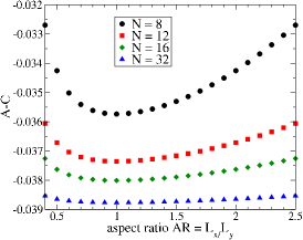
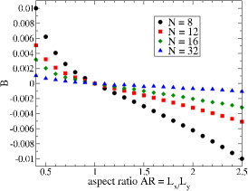
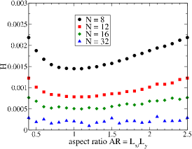
Figure 5: (a) Values of $A-C$ in Eq. (30) for a torus of $N_{\phi}=8,12,16,32$. The cutoff in momentum space was $|m|,|m^{\prime}|\leq 100N_{\phi}$. The value for an infinite system would be $-\frac{1}{32}\sqrt{\frac{\pi}{2}}\approx-0.039$. (b) The same for $B$ in Eq. (30). This term would vanish for the infinite system. (c) The same for $H$ in Eq. (30). This term would vanish for the infinite system.

Finally we have :

$$\frac{E_{\textrm{\scriptsize HF}}}{N\left(\frac{e^{2}}{\epsilon\ell}\right)}=-\epsilon_{N}+\frac{h+H}{2}\cos\theta+(A-|B|)\sin^{2}\theta+C\cos^{2}\theta.$$

This energy is minimized by $\cos\theta=\frac{h+H}{4(A-C-|B|)}$. Fig. 6 shows the $\theta$ angle that corresponds to the pseudospin polarization as a function of the bias $\frac{h\epsilon\ell}{e^{2}}$ at fixed aspect ratio, as well as the function of the aspect ratio at fixed bias values.

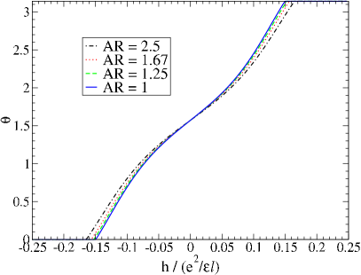
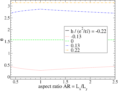
Figure 6: Left panel: The $\theta$ angle of the uniform state that corresponds to the pseudospin polarization as a function of the bias $h$ at fixed aspect ratio for $N_{\phi}=12$. Right panel: $\theta$ as a function of the aspect ratio at fixed bias.

We conclude that the finite system size hardly changes the Hartree-Fock prediction that the uniform phase exhibits orbital coherence in a wide range of the orbital bias, $-0.15\lesssim h\lesssim 0.15$, irrespective from the aspect ratio. The deviation of the orbital polarization for system sizes accessible in exact diagonalization from the thermodynamic limit is small.

VI Exact diagonalization results

We now expose results from our studies using exact diagonalization for a small number of electrons in the torus geometry, as defined in Sec. IV. The matrix elements of the Coulomb interaction among the single-body states in Eqs. (14) and (IV) are

$$\mathcal{A}_{j_{1},j_{2},j_{3},j_{4}}^{n_{1},n_{2},n_{3},n_{4}}=\frac{1}{L_{x}L_{y}}\sum_{n,m}^{\prime}\,\,\frac{2\pi e^{2}}{\epsilon q}\,\,{\mathrm{e}}^{-\frac{1}{2}(q_{x}^{2}+q_{y}^{2})}\,\,{\mathrm{e}}^{2i\pi\frac{n}{N_{\phi}}(j_{1}-j_{3})}\,\,F_{n_{1},n_{4}}(q_{x},q_{y})F_{n_{2},n_{3}}(-q_{x},-q_{y})\delta^{\prime}_{j_{1}+j_{2},j_{3}+j_{4}}\,\,\delta^{\prime}_{m,j_{1}-j_{4}}$$ (31)

where the sum over $n,m$ also includes momenta given by $q_{x}=2\pi n/L_{x},q_{y}=2\pi m/L_{y}$, and $\delta^{\prime}_{n,m}$ stands for Kronecker delta modulo $N_{\phi}$. The prime over the double sum means that we omit the $n=m=0$ term i.e. the $q_{x}=q_{y}=0$ contribution of the Coulomb potential due to the neutralizing background. The form factors $F_{n_{1}n_{2}}(q_{x},q_{y})$ encapsulate the dependence upon orbital index $n_{i}$ :

$$F_{00}=1,\quad F_{11}(q_{x},q_{y})=1-\frac{1}{2}(q_{x}^{2}+q_{y}^{2}),$$ (32)

$$F_{01}=-\frac{\ell}{\sqrt{2}}(iq_{x}+q_{y}),\quad F_{10}=-\frac{\ell}{\sqrt{2}}(iq_{x}-q_{y}).$$ (33)

Static effects of screening can be taken into account by multiplying the Coulomb potential $2\pi e^{2}/q$ by an appropriate function. The Hamiltonian we diagonalize is thus given by :

$$\mathcal{H}=\frac{1}{2}\sum_{n_{i},j_{i}}\mathcal{A}_{j_{1},j_{2},j_{3},j_{4}}^{n_{1},n_{2},n_{3},n_{4}}c^{\dagger}_{n_{1},j_{1}}c^{\dagger}_{n_{2},j_{2}}c_{n_{3},j_{3}}c_{n_{4},j_{4}}+hN_{1}$$ (34)

where the pseudomagnetic field $h$ parameterize the bare splitting between $n=0$ and $n=1$ Landau levels.

If we consider the particle-hole symmetry then the Hamiltonian Eq.(34) undergoes the change of field :

$$+hN_{1}\rightarrow-(h+\Delta_{0}+\Delta_{1})N_{1},$$ (35)

which implies that particle-hole symmetry requires the change $h\rightarrow h_{c}-h$ with a special critical field $h_{c}=-1/2(\Delta_{0}+\Delta_{1})$ which is non zero.

The algebra of magnetic translations can be used by build many-body conserved momenta FDM , allowing to factor out the degeneracy due to the center of mass momentum. If we have $N_{e}$ electrons at flux $N_{\phi}$ then one defines $N\equiv N_{e}/N_{\phi}$ the GCD when the filling fraction is $p/q$ i.e. $N_{e}/N_{\phi}\equiv pN/qN$ and $p$ and $q$ are coprime. There are two conserved momenta $K_{x},K_{y}$ that are living in a Brillouin zone and are discrete. We define two conserved integer quantum numbers $s,t$ by :

$$\mathrm{K}_{x}=\frac{2\pi}{L_{x}}s\,,\quad\mathrm{K}_{y}=\frac{2\pi}{L_{y}}t$$ (36)

where $s,t$ can be taken to vary in the interval $(0,N-1)$ because there is a period $N$ i.e. $s+N\equiv s$, $t+N\equiv t$. The modulus of the many-body momentum vector is then given by :

$$K=\sqrt{K_{x}^{2}+K_{y}^{2}}=\sqrt{\frac{2\pi}{N_{\phi}}}\sqrt{\frac{s^{2}}{\mathrm{AR}}+t^{2}\times\mathrm{AR}}.$$ (37)

One can now plot the eigenstates vs the total momentum $K$. The quantum numbers $s,t$ form a grid of $N^{2}$ points but in fact due to discrete symmetries many of them are symmetry-related. Notably there are symmetries with respect to $s\rightarrow N-s$ and $t\rightarrow N-t$ that are the discrete symmetries of the rectangular unit cell. As a consequence it is enough to get spectra in the region $s,t=0,\dots N/2$ since reflections lead then to all states.

There is a subtlety to note : the origin of the quantum numbers $s,t$ is not always zero. In fact when $pq(N_{e}-1)=2k+1$ then the origin should be taken as $s_{0},t_{0}=N/2$ while otherwise, $pq(N_{e}-1)=2k$ the origin is zero. It means that one has to include a shift of N/2 in the momentum definition Eq.(2). This is important in practice but has no other consequences.

The way we analyze numerical results is as follows : the nature of the phase of the system is set by the value of the control parameters in the projected Hamiltonian. In our case it is the pseudofield $h$ and any kind of screening parameter modifying the Coulomb interaction. For fixed parameters we put the system on a rectangle whose aspect ratio can be chosen at will. This change will not tune the nature of the phase. However some phases may be revealed more easily for some special aspect ratio. In the case of incompressible fluid states exhibiting the FQHE it is known that they are very insensitive to the geometry as expected for a liquid state of matter. On the contrary states which break translation symmetries are very sensitive to the aspect ratio. It is by fine tuning that one can observe a set of quasi-degenerate states that are the hallmark of broken translation symmetry RHY ; HRY ; YHR . This happens in the case of the Wigner crystal state at low filling factors in the LLL and also in the case of stripe states observed at half-filling in high enough LLs. When the aspect ratio is not tuned to the optimal value then the spectrum is featureless as expected for a compressible system.

VII Polarized incoherent phase

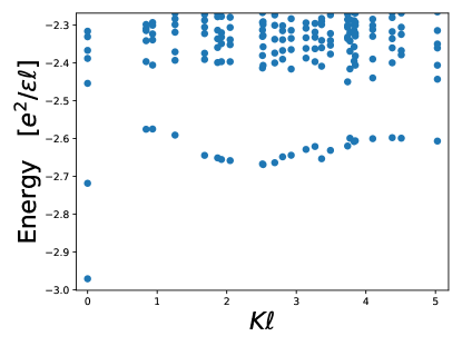
Figure 7: Exact eigenstates of a $N_{e}=8$ electron system at $\nu=1$ when the bare splitting h favors the accumulation into the LLL. The first excited states are expected to be magneto-excitons obtained by promoting a single electron into the $n=1$ LL. This consistent with the well-defined excitation branch above the $K=0$ ground state. Here the aspect ratio is tuned to $\mathrm{AR}=1$. The branch is flatter when we increase the $n=0$/$n=1$ splitting given by the field $h$.

When the splitting between the two $n=0/n=1$ Landau levels is very large, then the physics becomes simple. If for example the $n=1$ states are at very large energy then the $\nu=1$ ground state is obtained by filling all orbitals of the $n=0$ levels. For $\nu=1$ there is only one way to do it and this leads to a single Slater determinant. As a consequence this state is uniform and has total momentum $K=0$. Excited states are also simple. The first excited state is obtained by promoting only one electron in the upper $n=1$ band. As can be observed in Figure (7) there is a well-defined collective mode that we interpret as the magnetoexciton. This magnetoexciton has a dispersion that can be computed by standard analytical techniques. Within random-phase approximation the dispersion relation is given by the zeroes of $1-v_{q}\chi_{0}(q,\omega)$ where $v_{q}=2\pi e^{2}/\epsilon q$ is the Fourier transform of the Coulomb potential and $\chi_{0}(q,\omega)$ the so-called Lindhard function :

$$\chi_{0}(q,\omega)\equiv\frac{1}{2\pi}\sum_{j,j^{\prime}}|F_{jj\prime}(q)|^{2}\frac{n(\varepsilon_{j})-n(\varepsilon_{j}^{\prime})}{\hbar\omega+(j-j^{\prime})h+i\eta}=\frac{e^{-q^{2}\ell^{2}/2}}{2\pi}(\frac{q^{2}}{2})\left[\frac{1}{\hbar\omega-h+i\eta}-\frac{1}{\hbar\omega+h+i\eta}\right],$$ (38)

where $n(\varepsilon)$ is the occupation number and $\eta$ a vanishing regulator. This leads to the RPA formula :

$$\omega^{RPA}_{q}=h+(\frac{e^{2}}{\epsilon\ell})\frac{1}{2}q\ell\,e^{-q^{2}\ell^{2}/2}$$ (39)

It is also possible to derive the time-dependent Hartree-Fock dispersion relation following the treatment of full Landau levels GiulianiVignale  :

$$\omega^{TDHF}_{q}=h+(\frac{e^{2}}{\epsilon\ell})q\ell\,e^{-q^{2}\ell^{2}/2}+(\frac{e^{2}}{\epsilon\ell})\int_{0}^{\infty}dx\,e^{-x^{2}/2}(1-L_{1}(\frac{x^{2}}{2}))-(\frac{e^{2}}{\epsilon\ell})\int\frac{d\mathbf{w}}{2\pi}\frac{e^{-w^{2}/2}}{|\mathbf{w}+\mathbf{q}\ell\times\mathbf{{\hat{z}}}|}\frac{w^{2}}{2}$$ (40)

which leads to the following explicit formula :

$$\omega^{TDHF}_{q}=h+(\frac{e^{2}}{\epsilon\ell})q\ell\,e^{-q^{2}\ell^{2}/2}-(\frac{e^{2}}{\epsilon\ell})\frac{1}{4}\sqrt{\frac{\pi}{2}}e^{-q^{2}\ell^{2}/4}q^{2}\ell^{2}\left[I_{0}(\frac{q^{2}\ell^{2}}{4})-I_{1}(\frac{q^{2}\ell^{2}}{4})\right]+(\frac{e^{2}}{\epsilon\ell})\frac{1}{2}\sqrt{\frac{\pi}{2}}\left[1-e^{-q^{2}\ell^{2}/4}I_{0}(\frac{q^{2}\ell^{2}}{4})\right]$$ (41)

These two dispersion relations tend to $\omega=h$ when $q\rightarrow 0$ which a remnant of Kohn theorem in this system restricted to two LLs. However we note that the behavior at large momentum is very different between RPA and TDHF. While $\omega^{RPA}_{q}\rightarrow h$ for $q\rightarrow\infty$ the TDHF result goes to a finite limit greater than $h$. Indeed for large momentum the separation between the electron and its associated hole depends on the quantity $\mathbf{q}\ell\times\mathbf{{\hat{z}}}$ which is the separation between them in units of $\ell$ so for large $q$ the electron and hole are far apart and the energy of the magneto-exciton approaches the sum of the HF energies of the two particles plus their Coulomb interaction $-e^{2}/(\epsilon q\ell^{2})$. This is behavior is observed in our ED studies. In Fig.(8) for $h=5\times e^{2}/(\epsilon\ell)$ we see that the RPA fails to reproduce the large momentum behavior while the TDHF approximation is in good agreement with ED results. However this is true only in the large splitting $h$ limit.

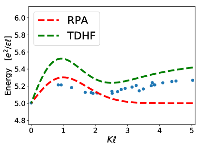
Figure 8: Dispersion of the collective mode in the incoherent phase. Here we have $N_{e}=8$ electrons at aspect ratio 0.9 and the level splitting is taken to be $h/(e^{2}/(\epsilon\ell))=5$. The ED points are blue discrete points while RPA approximation to the magneto-exciton is the red line and the TDHF result is green.

The HF theory thus predicts that the incoherent polarized state would become unstable for $h<0$. We find instead that the incoherent phase is stable up to negative values of the bare field $h_{c1}\approx-0.1e^{2}/(\epsilon\ell)$ and also by use of the particle-hole symmetry discussed in section III it extends also from the symmetric field from $h_{c}=-\infty$ to $h_{c2}\approx-0.2$. This means that the special case with $h=0$ is in fact within the incoherent phase, in agreement with the findings of Ref. (AbaninPapic, ). The excitation spectrum is just a distortion of that in Fig.(7). A hypothetical uniform orbitally coherent phase would be accompanied by a Goldstone mode Barlas08 ; Barlas10 ; Cote10 ; Cote11 . We do not observe such a softening of the low-lying excitations. Instead, as we will see in the next section, we find evidence for a phase that breaks spontaneously translation symmetry.

VIII Helical phase

The incoherent phase is quite insensitive to the aspect ratio of the rectangular system. If now we tune the field $h$ to negative values we observe a change of behavior. The ground state is no longer at zero momentum and its location in the Brillouin zone depends on the aspect ratio. We have varied the aspect ratio to find the characteristic behavior of the system. Typical spectra are displayed in Fig.(9). There is a range of aspect ratio close to 0.3-0.4 for which the ground state becomes degenerate and excited states appear clearly above as a discrete set of states. These states have many-body momenta that differ by a one-dimensional wavevector : see Fig.(10). This is the behavior expected from a quantum system that breaks a symmetry as observed previously in quantum Hall systems HRY ; RHY ; YHR . There is a characteristic wavevector associated from this manifold of states which is the momentum difference of the low-lying states. It is important to note that the region in aspect ratio where this degeneracy appears is not adiabatically connected to the thin-torus of AR going to zero. There are many level crossings before this limit so the helical phase we observe is not a simple electrostatic limit of the quantum Hall problem but a real nontrivial many-body state. We have also checked that these spectral features are stable if we distort the torus into an oblique cell.

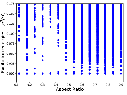
Figure 9: Excitation gap above the $K=0$ ground state of $N_{e}=10$ electrons as a function of the aspect ratio. The pseudomagnetic field is tuned at the particle-hole invariant value which is in the middle of the helical phase. The ground state degeneracy is clear when the aspect ratio is close to 0.35.

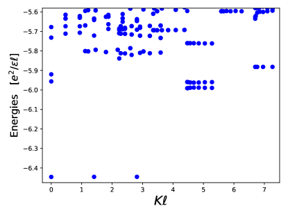
Figure 10: Spectrum of $N_{e}=12$ electrons for aspect ratio 0.45. The pseudomagnetic field is tuned at the particle-hole invariant value which is in the middle of the helical phase. The ground state degeneracy is evidence for a state with spontaneously broken translation symmetry.

To pin down the phase boundary of the helical phase we have used two indicators. The first one is the value of the orbital polarization of the ground state in the $K=0$ sector. We define it as the normalized population of the $n=1$ orbitals:

$$\mathcal{P}=\langle\Psi|N_{1}|\Psi\rangle/N_{e},$$ (42)

so that $0\leq\mathcal{P}\leq 1$ and the polarization goes to zero for large positive $h$ and goes to unity for large negative $h$. We expect that by the particle-hole symmetry the curve has a center of symmetry for a non-trivial value of the field. This is exactly what we observe. See Fig.(11) for the polarization of 10 electrons in a rectangle of aspect ratio 0.9. Here we have used the polarization of the ground state in the $K=0$ sector. This does not mean that this state remains the strict absolute ground state for all values of $h$ and also for various values of the aspect ratio. Note also that in the incoherent phases for large $h$ values the polarization is either small or close to unity but remains nontrivial as expected from conventional perturbative considerations.

The other indicator for phase transitions is the quantum fidelity of the ground state. This is computed by changing the $h$ field by a small value and computing the overlap between the ground states for these neighboring values :

$$\mathcal{F}=\langle\Psi(h)|\Psi(h+\epsilon)\rangle.$$ (43)

We have computed the fidelity as a function of $h$ for an aspect ratio fixed to 0.9. It varies very weakly in the fully polarized phase and has strong variations only at what we define as the helical state. See Fig.(12) where we display data for $N=14$ electrons. The apparent two-peak structure allows us to define finite-system critical values by taking the $h$ values where the fidelity has peaks. This is an alternate way to characterize phase boundaries of the helical state. We do not have access to enough system sizes to perform a meaningful finite-size scaling of the fidelity.

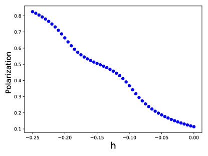
Figure 11: The polarization of the ground state as a function of the field $h$ for aspect ratio 0.9 and 10 electrons.

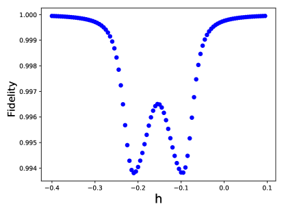
Figure 12: The quantum fidelity $\mathcal{F}$ of the $K=0$ ground state as a function of the field $h$ for aspect ratio 0.9 and 14 electrons.

The boundaries of the helical phase can thus be pinned down either by looking at the maximum value of the derivative of the polarization Eq.(42) or also at peak fidelity Eq.(43). These two estimators are plotted in Fig.(13) as a function of the inverse system size. By use of a linear fit we obtain $h_{c1}\approx-0.1$ and $h_{c2}\approx-0.22$. Changing the aspect ratio slightly changes these values and associated uncertainty is estimated to be of the same order at that coming from the extrapolation to the thermodynamic limit.

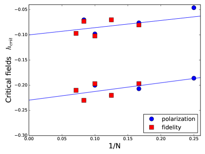
Figure 13: The two critical field delimiting the stability region of the helical phase. The values are plotted as a function of the inverse system size. The blue circles are obtained from the maximum derivative of the polarization defined in Eq.(42) and the red squares from the peak values of the fidelity defined in Eq.(43)

IX Conclusions

By means of exact diagonalization on the torus, we have shown that at filling factor $\nu=1$ a system of two Landau levels with orbital character $n=0/1$ exhibits a non-trivial ground state with spontaneously broken translational symmetry that is stabilized by a orbital single particle splitting ($h$), within the range $-0.1\gtrsim h\gtrsim-0.22$. Here negative $h$ favors polarization into the $n=1$LL. This state is consistent with the orbitally coherent ferroelectric helical phase that was identified in previous Hartree-Fock studies Barlas08 ; Barlas10 ; Cote10 ; Cote11 ; Lambert ; Knothe . Outside of this range of orbital splittings the system has an incoherent ground state that is adiabatically connected to the trivial fully polarized states into the $n=0/1$ orbitals depending on the sign of $h$, including the case of $h=0$ previously studied in Ref. (AbaninPapic, ). The low lying excitations of these incoherent states are well captured by TDHF to a precision of a few percent.

We observe a direct transition from this incoherent state into the broken translational symmetry state. Aside from the incoherent and the broken translational symmetry phases phases, we see no evidence for a potential uniform state with orbital coherence, and, in particular, we do not observe the appearance of its characteristic Goldstone mode. The location of the helical phase is in rough agreement with HF predictions, whose boundaries we pin using two criteria: quantum fidelity and polarization change. Therefore, we conclude that while HF correctly predicts a helical phase it overestimates the tendency to uniform orbital coherent state.

Using a model that includes all the single particle splittings of BLG, we estimate that the orbital splittings can be effectively tuned by applying an interlayer electric bias. Our estimates indicate that there is a realistic prospect to achieve the regime in which the ferroelectric helical phase becomes the ground state in current experiments Hunt ; Andrea2017 ; Dean by applying a large interlayer bias on the order of $u\sim 80{\rm meV}$.

- (1) K. S. Novoselov, A. K. Geim, S. V. Morozov, D. Jiang, M. I. Katsnelson, I. V. Grigorieva, S. V. Dubonos, A. A. Firsov, Nature 438, 197 (2005).
- (2) K. S. Novoselov, E. McCann, S. V. Morozov, V. I. Fal’ko, M. I. Katsnelson, U. Zeitler, D. Jiang, F. Schedin, and A. K. Geim, Nature Physics 2, 177 (2006).
- (3) X. Du, I. Skachko, F. Duerr, A. Luican, E. Y. Andrei, Nature 462, 192 (2009).
- (4) K. I. Bolotin, F. Ghahari, M. D. Shulman, H. L. Stormer, P. Kim, Nature 462, 196 (2009).
- (5) C. R. Dean et al., Nature Physics 7, 693 (2011).
- (6) Benjamin E. Feldman, Benjamin Krauss, Jurgen H. Smet, Amir Yacoby, Science 337, 1196 (2012).
- (7) D. S. Lee, V. Skakalova, R. T. Weitz, K. von Klitzing, and J. H. Smet, Phys. Rev. Lett. 109, 056602 (2012).
- (8) A. F. Young, C. R. Dean, L. Wang, H. Ren, P. Cadden-Zimansky, K. Watanabe, T. Taniguchi, J. Hone, K. L. Shepard, and P. Kim, Nature Physics 8, 550-556 (2012).
- (9) A. H. Castro Neto et al., Rev. Mod. Phys. 81, 109 (2009).
- (10) D. A. Abanin, S. A. Parameswaran, S. L. Sondhi, Phys. Rev. Lett. 103, 076802 (2009).
- (11) D. A. Abanin, B. E. Feldman, A. Yacoby, and B. I. Halperin, Phys. Rev. B88, 115407 (2013).
- (12) C. Tőke and J. K. Jain, Phys. Rev. B75, 245440 (2007).
- (13) D.-K. Ki, V. I. Fal’ko, D. A. Abanin, and A. F. Morpurgo, Nano Letters 14, 2135 (2014).
- (14) Z. Papić, D. A. Abanin, Y. Barlas, and R. N. Bhatt, Phys. Rev. B84, 241306(R) (2011).
- (15) D. A. Abanin, Z. Papić, Y. Barlas, and R. N. Bhatt, New J. Phys. 14, 025009 (2012).
- (16) E. McCann and V. I. Fal’ko, Phys. Rev. Lett.96, 086805 (2006).
- (17) K. Yang, S. Das Sarma, and A. H. MacDonald, Phys. Rev. B74, 075423 (2006).
- (18) Y. Barlas, R. Côté, K. Nomura, and A. H. MacDonald, Phys. Rev. Lett. 101,097601(2008).
- (19) Y. Barlas, R. Côté, J. Lambert, and A. H. MacDonald, Phys. Rev. Lett. 104, 096802 (2010).
- (20) R. Côté, J. Lambert, Y. Barlas, and A. H. MacDonald, Phys. Rev. B82, 035445 (2010).
- (21) R. Côté, J. P. Fouquet, and W. Luo, Phys. Rev. B84, 235301 (2011).
- (22) J. Lambert and R. Côté, Phys. Rev. B87, 115415 (2013).
- (23) A. Knothe and Th. Jolicoeur, Phys. Rev. B94, 235149 (2016).
- (24) I. Sodemann, Z. Zhu, and L. Fu, Phys. Rev. X 7, 041068 (2017).
- (25) Z. Papić and D. A. Abanin, Phys. Rev. Lett. 112, 046602 (2014).
- (26) K. Shizuya, Phys. Rev. B86, 045431 (2012).
- (27) B. M. Hunt, J. I. A. Li, A. A. Zibrov, L. Wang, T. Taniguchi, K. Watanabe, J. Hone, C. R. Dean, M. Zaletel, R. C. Ashoori and A. F. Young, Nature Communications 8, 948 (2017).
- (28) A. A. Zibrov, C. Kometter, H. Zhou, E. M. Spanton, T. Taniguchi, K. Watanabe, M. P. Zaletel and A. F. Young, Nature 549, 360 (2017).
- (29) J. I. A. Li, C. Tan, S. Chen, Y. Zeng, T. Taniguchi, K. Watanabe, J. Hone, C. R. Dean, Science 358, 648 (2017).
- (30) J. Jung and A. H. MacDonald, Phys. Rev. B89, 035405 (2014).
- (31) J. Zak, Phys. Rev. 134, A1602 (1964).
- (32) T. Haidekker Galambos and C. Tőke, Phys. Rev. E97, 022140 (2018).
- (33) D. Mumford, Tata Lectures on Theta I, Springer (1987).
- (34) F. D. M. Haldane, Phys. Rev. Lett. 55, 2095 (1985).
- (35) E. H. Rezayi, F. D. M. Haldane, and Kun Yang, Phys. Rev. Lett. 83, 1219 (1999).
- (36) F. D. M. Haldane, E. H. Rezayi, and Kun Yang, Phys. Rev. Lett. 85, 5396 (2000).
- (37) Kun Yang, F. D. M. Haldane, and E. H. Rezayi, Phys. Rev. B64, 081301(R) (2001).
- (38) G. F. Giuliani and G. Vignale, “Quantum Theory of the Electron Liquid”, Cambridge University Press, Cambridge UK. see p. 585 for the TDHF treatment of full Landau levels.