Collider and Gravitational Wave Complementarity in Exploring the Singlet Extension of the Standard Model

Abstract

We present a dedicated complementarity study of gravitational wave and collider measurements of the simplest extension of the Higgs sector: the singlet scalar augmented Standard Model. We study the following issues: $(i)$ the electroweak phase transition patterns admitted by the model, and the proportion of parameter space for each pattern; $(ii)$ the regions of parameter space that give detectable gravitational waves at future space-based detectors; and $(iii)$ the current and future collider measurements of di-Higgs production, as well as searches for a heavy weak diboson resonance, and how these searches interplay with regions of parameter space that exhibit strong gravitational wave signals. We carefully investigate the behavior of the normalized energy released during the phase transition as a function of the model parameters, address subtle issues pertaining to the bubble wall velocity, and provide a description of different fluid velocity profiles. On the collider side, we identify the subset of points that are most promising in terms of di-Higgs and weak diboson production studies while also giving detectable signals at LISA, setting the stage for future benchmark points that can be used by both communities.

1 Introduction

Since the first direct detection of gravitational waves (GWs) by the LIGO and Virgo collaborations Abbott:2016blz , a new interface has arrived in particle physics – its intersection with GW astronomy. While ground based GW detectors have their best sensitivity at frequencies $\sim\mathcal{O}(100)\,\text{Hertz}$ and their main targets are black hole and neutron star binaries, there is now growing interest in building space-based interferometer detectors for milli-Hertz or deci-Hertz frequencies. Many detectors have been proposed, such as the Laser Interferometer Space Antenna (LISA) Audley:2017drz , the Big Bang Observer (BBO), the DECi-hertz Interferometer Gravitational wave Observatory (DECIGO) Yagi:2011wg , Taiji Gong:2014mca and Tianqin Luo:2015ght . The physical sources of GWs in this frequency band include supermassive black hole binaries Klein:2015hvg , extreme mass ratio inspirals Babak:2017tow and the stochastic background of primordial GWs produced during first order cosmological phase transitions Caprini:2015zlo .

This offers tremendous opportunities for theorists, as a new window to the early Universe opens up. Aspects of dark sector physics and baryon asymmetry can now be framed fruitfully in a language that lends itself to data from the GW frontier. The key connection is phase transitions, which on the one hand are a primary target of future GW experiments, and on the other are important features of scalar potentials and hence have historically been the target of collider physics.

The purpose of our work is to explore the complementarity of future GW detectors and future particle colliders in probing phase transitions in the early Universe – in the simplest particle physics setting possible, but also with great attention to details within such a setting. The natural choice is the electroweak phase transition (EWPT)  Grojean:2006bp with the simplest extension of the Higgs sector: the singlet scalar augmented Standard Model or the xSM. This model is capable of providing a strongly first order EWPT through a tree level barrier and is the simplest model in Class IIA of the tree level renormalizable operators described in Chung:2012vg (see Ref. Beniwal:2018ygo ; Croon:2018kqn ; Hashino:2018wee ; Marzo:2018nov ; Beniwal:2017eik ; Hashino:2018zsi ; Addazi:2017gpt ; Addazi:2017nmg ; Chiang:2017zbz ; Wan:2018udw ; Chen:2017cyc ; Vieu:2018nfq ; Basler:2017uxn ; Jinno:2017ixd ; Chao:2017ilw ; Huang:2014ifa ; Tsumura:2017knk ; Bian:2017wfv ; Hektor:2018esx ; Huang:2017rzf ; Ghorbani:2017lyk ; Kang:2017mkl ; Addazi:2017oge ; Chen:2017qcz ; Marzola:2017jzl ; Kobakhidze:2017mru ; Zhou:2018zli ; Beniwal:2018hyi ; Dev:2016feu ; Balazs:2016tbi ; Ahriche:2018rao ; Shajiee:2018jdq ; Bian:2018bxr ; Blinov:2015sna ; Inoue:2015pza ; Vaskonen:2016yiu ; No:2018fev ; Chiang:2018gsn ; Chala:2018opy ; Cai:2017tmh ; Alanne:2018brf ; Kannike:2019wsn ; Ashoorioon:2009nf ; Cheng:2018ajh ; Bi:2015qva for related studies on EWPT and GW). It has been extensively investigated in phenomenological studies Profumo:2007wc ; Profumo:2014opa ; Huang:2017jws ; Robens:2015gla , studies of EWPT Profumo:2014opa ; Profumo:2007wc ; Kotwal:2016tex ; Espinosa:2011ax ; Kozaczuk:2015owa and di-Higgs analyses Lewis:2017dme guided by the requirements of EWPT Huang:2017jws , and electroweak baryogenesis (EWBG).

We perform a detailed scan of this model, shedding light on the following issues: $(i)$ the EWPT patterns admitted by the model, and the proportion of parameter space for each pattern; $(ii)$ the regions of parameter space that give detectable GWs at future space-based detectors; $(iii)$ the current and future collider measurements of di-Higgs production, as well as searches for a heavy weak diboson resonance, and how these searches interplay with regions of parameter space that exhibit strong GW signals; and $(iv)$ the complementarity of collider and GW searches in probing this model.

We first carefully work out and incorporate all phenomenological constraints: boundedness of the Higgs potential from below, electroweak vacuum stability at zero temperature, perturbativity, perturbative unitarity, Higgs signal strength measurements and electroweak precision observables. Then, we identify the regions of parameter space which give large signal-to-noise-ratio (SNR) at LISA. We carefully address subtle issues pertaining to the bubble wall velocity $v_{w}$, making a distinction between $v_{w}$, which enters GW calculations, and the velocity $v_{+}$ that is used in EWBG calculations. The relation between these two velocities is determined from a hydrodynamic analysis by solving the velocity profile surrounding the bubble wall. We provide a description of different fluid velocity profiles and investigate the behavior of the normalized energy released during the phase transition, $\alpha$, which primarily determines the SNR, as a function of the model parameters. On the collider side, we identify the subset of points with large SNR at LISA that are most promising in terms of di-Higgs and weak diboson production studies, setting the stage for future benchmark points.

Much remains to be understood about the Higgs sector. On the collider side, measuring the Higgs cubic and quartic couplings through double or triple Higgs production, both non-resonant as well as resonant, is an extremely difficult but central goal of future experiments (see e.g., Azatov:2015oxa ; Alves:2017ued ; DiVita:2017vrr ; Plehn:2005nk ; Binoth:2006ym ; Bizon:2018syu ; Liu:2018peg ). While any deviation of the shape of the Higgs potential from what is expected within the Standard Model (SM) would hint to new physics, the sensitivities of such collider studies are found to be rather low. The detection of GWs from EWPT in future experiments can offer a complementary method of probing the currently largely unknown Higgs potential. Our work is a step in that direction.

The paper is structured as follows. In Sec. 2, we define the Higgs potential and set the notations. The standard phenomenological analysis is discussed in the following Sec. 3. The next Sec. 4 discuss the details of the EWPT and GW calculations, after which the results and discussions from the full scan is presented in Sec. 5 and we summarize in Sec. 6.

2 The Model

In this section, we fix our notation by defining the potential for the gauge singlet extended SM, known as the“xSM”. This model is defined with the following potential setup Profumo:2007wc ; Profumo:2014opa ; Huang:2017jws :

$$V(H,S) = -\mu^{2}H^{\dagger}H+\lambda(H^{\dagger}H)^{2}+\frac{a_{1}}{2}H^{\dagger}HS$$ (1)

$$+\frac{a_{2}}{2}H^{\dagger}HS^{2}+\frac{b_{2}}{2}S^{2}+\frac{b_{3}}{3}S^{3}+\frac{b_{4}}{4}S^{4},$$

where $H^{\text{T}}=(G^{+},(v_{\text{EW}}+h+iG^{0})/\sqrt{2})$ is the SM Higgs doublet and $S=v_{s}+s$ the real scalar gauge singlet. All the model parameters in the above equation are real. The parameters $\mu$ and $b_{2}$ can be solved from the two minimization conditions around the EW vacuum($\equiv(v_{\text{EW}},v_{s})$),

$$\mu^{2}=\lambda v_{\text{EW}}^{2}+\frac{1}{2}v_{s}(a_{1}+a_{2}v_{s}),$$

$$b_{2}=-\frac{1}{4v_{s}}[v_{\text{EW}}^{2}(a_{1}+2a_{2}v_{s})+4v_{s}^{2}(b_{3}+b_{4}v_{s})],$$ (2)

and $\lambda,a_{1},a_{2}$ can be replaced by physical parameters $\theta$, $m_{h_{1}}$ and $m_{h_{2}}$ from the mass matrix diagonalization :

$$\lambda=\frac{m_{h_{1}}^{2}c_{\theta}^{2}+m_{h_{2}}^{2}s_{\theta}^{2}}{2v_{\text{EW}}^{2}},$$

$$a_{1}=\frac{2v_{s}}{v^{2}_{\text{EW}}}[2v_{s}^{2}(2b_{4}+\tilde{b}_{3})-m_{h_{1}}^{2}-m_{h_{2}}^{2}+c_{2\theta}(m_{h_{1}}^{2}-m_{h_{2}}^{2})],$$

$$a_{2}=\frac{-1}{2v_{\text{EW}}^{2}v_{s}}[-2v_{s}(m_{h_{1}}^{2}+m_{h_{2}}^{2}-4b_{4}v_{s}^{2})$$

$$\hskip 56.9055pt+(m_{h_{1}}^{2}-m_{h_{2}}^{2})(2c_{2\theta}v_{s}-v_{\text{EW}}s_{2\theta})+4\tilde{b}_{3}v_{s}^{3}],$$ (3)

where $\tilde{b}_{3}\equiv b_{3}/v_{s}$ and we have defined the physical fields $h_{1}$ and $h_{2}$ as

$$h_{1}=c_{\theta}h+s_{\theta}s,\quad\quad h_{2}=-s_{\theta}h+c_{\theta}s,$$ (4)

with a mixing angle $\theta$. We note that $h_{1}$ is identified as the SM Higgs while $h_{2}$ is a heavier scalar. The coupling of $h_{1}$ with the SM particles is reduced by a factor of $c_{\theta}$ while the coupling of $h_{2}$ with SM particles is $(-s_{\theta})$ times the corresponding SM couplings and vanishes in the case of zero mixing angle.

With choices of parameter transformations described above, the potential is fully specified by the following five parameters:

$$\centering v_{s},\quad\quad m_{h_{2}},\quad\quad\theta,\quad\quad b_{3},\quad\quad b_{4}.\@add@centering$$ (5)

The model defined here has several variants in the literature. For example, since the potential can be defined with a translation in the $S$ direction $S\rightarrow S^{\prime}=S-v_{s}$, such that $\langle S\rangle=0$, the resulting potential will take the same form as Eq. 1 but with the addition of a non-zero tadpole term $b_{1}S$ Lewis:2017dme . The potential and physics remain the same but the parameters in the potential will transform accordingly. The transformation rules to and from this basis are given in Appendix  B. There is also a variant where there is a spontaneously broken $Z_{2}$ symmetry $S\rightarrow-S$; this corresponds to a subset of the parameter space here where $a_{1}=b_{3}=0$.

We further note that we do not include CP-violation in this study since the magnitude of the CP-violation is typically very constrained by current electric dipole moment searches (e.g., Inoue:2014nva ; Chen:2017com ; Bian:2017wfv or the included CP-violation may be large but has little effect on EWPT Guo:2016ixx ).

3 Phenomenological Constraints

In this section, we briefly discuss the phenomenological constraints used in our analysis, following the standard treatments given in Refs. Pruna:2013bma ; Robens:2015gla ; Lewis:2017dme . The phenomenological discussion includes boundedness of the Higgs potential from below, EW vacuum stability at zero temperature, perturbativity, perturbative unitarity, Higgs signal strength measurements and electroweak precision observables.

First, the potential needs to be bounded from below. Requiring this for arbitrary field directions gives us the condition Lewis:2017dme  ,

$$\lambda>0,\quad b_{4}>0,\quad a_{2}\geqslant-2\sqrt{\lambda b_{4}}.$$ (6)

Next, the EW vaccum also needs to be stable at zero temperature. Using physical parameters as input will automatically guarantee that the EW vacuum is a minimum. To ensure that the above EW vacuum is stable, one should require that no deeper minimum exists in the potential. In our analysis, we find all the minima by firstly solving $\partial V/\partial\phi_{i}=0$($\phi_{1}\equiv h$, $\phi_{2}\equiv s$) and subsequently calculating eigenvalues of the Hessian matrix $\{\partial^{2}V/\partial\phi_{i}\partial\phi_{j}\}$ to determine the nature of the extrema for each set of parameter input.

Next, Higgs signal strength measurements in various channels require the couplings of $h_{1}$ to be not far from the SM Higgs couplings. In the xSM, the couplings of $h_{1}$ to SM particles are reduced by a factor of $\cos\theta$, therefore the Higgs signal strength is given by $\mu_{H}=\cos^{2}\theta$. Experimentally, the most recent ATLAS and CMS combined fit of this value is $\mu_{H}=1.09^{+0.11}_{-0.10}$ Khachatryan:2016vau and a $\chi^{2}$ analysis shows that $|\sin\theta|>0.33$ are excluded at $95\%$ CL Carena:2018vpt .

Moreover, unitarity puts constraints on the high energy behavior of particle scatterings. Requiring further the perturbativity of these scatterings at high energy will lead to constraints on the model. This tree level perturbativity requirement is quantified as the condition that the partial wave amplitude $a_{l}(s)$ for all $2\rightarrow 2$ processes satisfies $|\text{Re}\,a_{l}(s)|\lesssim 1/2$ for $\sqrt{s}\rightarrow\infty$. We consider all channels of scalar/vector boson $2\rightarrow 2$ scatterings at the leading order in the high energy expansion, with details of the S-matrix given in Appendix. A.

Electroweak precision measurements, which mainly include the $W$ boson mass measurement Lopez-Val:2014jva and the oblique EW corrections Peskin:1991sw ; Hagiwara:1994pw , put further constraints on the model. The $W$ boson mass $m_{W}$ can be calculated given experimentally measured values of $G_{F}$, $m_{Z}$ and the fine structure constant at zero momentum transfer $\alpha(0)$ Lopez-Val:2014jva . The function relating $m_{W}$ and these three parameters depends on the loop corrections of the vector boson self-energies. Comparing this calculated $m_{W}$ with the experimental measurement $m_{W}^{\text{exp}}=80.385\pm 0.015\text{GeV}$ Alcaraz:2006mx ; Aaltonen:2012bp ; D0:2013jba highly constrains the modification of the loop corrections by new physics effects. In this model, the modified loop corrections result from reduced Higgs couplings and from the presence of the heavier scalar $h_{2}$ and are only dependent on $(\theta,m_{h_{2}})$ at one-loop level. The same parameter dependence enters the oblique $S,T,U$ parameters and it turns out that the $W$-mass constraint is much more stringent than that from the oblique corrections Lopez-Val:2014jva ; Robens:2015gla .

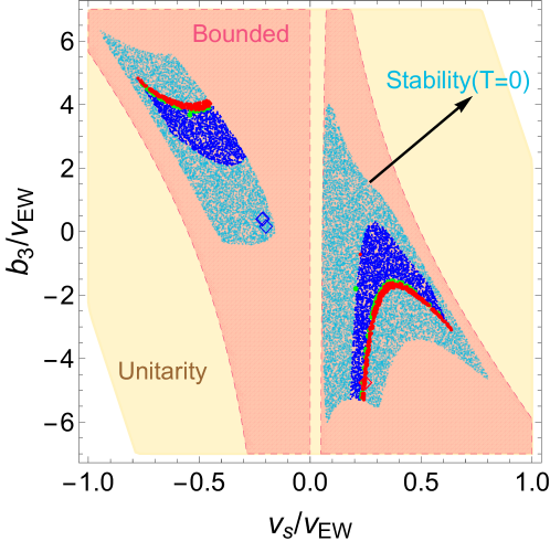
Figure 1: An illustrative plot showing various phenomenological constraints. The shaded regions are allowed by requirements of unitarity, boundedness of the potential from below, and stability of EW vacuum at zero temperature. Points are also overlapped on this plot where various EWPT criteria are fulfilled and with $\text{SNR}>50$ (red), $50>\text{SNR}>10$ (green) and $\text{SNR}<10$ (blue). The diamond-shaped points give two-step EWPT.

To give the reader a flavor of the above phenomenological constraints, we fix $m_{h_{2}}=300\,\text{GeV}$, $\theta=0.2$, $b_{4}=4$ and show the various bounds on the remaining two parameters $(v_{s}/v_{\text{EW}},b_{3}/v_{\text{EW}})$ in Fig. 1. This choice of $m_{h_{2}}$ and $\theta$ evades the constraints from the $W$-mass as well as the oblique EW corrections and regions outside the color-shaded regions are excluded by the remaining constraints. It can be seen from this figure that the least constraining condition comes from the perturbative unitarity requirement for this parameter choice. The bounded-from-below condition is more restrictive and also separates the plane into two disconnected regions while the stability of the EW vacuum at zero temperature shrinks the allowed parameter space even more. We also overlaid on this plot the points which pass the various EWPT requirements and give GW signals with varying SNR. More details are given in the caption and in the following section.

4 EWPT and Gravitational Waves

4.1 Effective Potential

EWPT is an essential step  in generating the observed baryon asymmetry in the universe by providing an out-of-equilibrium environment, one of the three Sakharov conditions Sakharov:1967dj , in the framework of electroweak baryogenesis (see Morrissey:2012db for a recent review). Augmented with the rapid baryon number violating Sphaleron process outside the electroweak bubbles and the CP-violating particle scatterings on the bubble walls, a net baryon number can be produced inside the bubbles. Aside from the particle interactions, which are used in EWBG calculations, the cosmological context that characterizes the dynamics of the EWPT can be calculated from the finite temperature effective potential. The standard procedure of calculating it includes adding the tree level effective potential, the Coleman-Weinberg term Coleman:1973jx and its finite temperature counterpart Quiros:1999jp as well as the daisy resummation Parwani:1991gq ; Gross:1980br . Since the EWPT in this model is mainly driven by the cubic terms in the potential and out of concern of a gauge parameter dependence Patel:2011th of the effective potential calculated in the above standard procedure, we take here the high temperature expansion approximation, which is gauge invariant, in line with previous analyses of this model Profumo:2007wc ; Profumo:2014opa ; Kotwal:2016tex ; Huang:2017jws ; Alves:2018oct . This effective potential is then given by 

$$V(h,s,T)=-\frac{1}{2}[\mu^{2}-\Pi_{h}(T)]h^{2}-\frac{1}{2}[-b_{2}-\Pi_{s}(T)]s^{2}$$

$$\hskip 19.91684pt+\frac{1}{4}\lambda h^{4}+\frac{1}{4}a_{1}h^{2}s+\frac{1}{4}a_{2}h^{2}s^{2}+\frac{b_{3}}{3}s^{3}+\frac{b_{4}}{4}s^{4},\quad\quad$$ (7)

where $\Pi_{h}(T)$ and $\Pi_{s}$ are the thermal masses of the fields,

$$\Pi_{h}(T)=\left(\frac{2m_{W}^{2}+m_{Z}^{2}+2m_{t}^{2}}{4v^{2}}+\frac{\lambda}{2}+\frac{a_{2}}{24}\right)T^{2},$$

$$\Pi_{s}(T)=\left(\frac{a_{2}}{6}+\frac{b_{4}}{4}\right)T^{2},$$ (8)

where the gauge and Yukawa couplings have been written in terms of the physical masses of $W$, $Z$ and the $t$-quark. With this effective potential, the thermal history of the EW symmetry breaking can be analyzed. It depends mainly on the following key parameters:

$$\centering T_{c},\quad T_{n},\quad\alpha,\quad\beta,\quad v_{w}.\@add@centering$$ (9)

Here $T_{c}$ is the critical temperature at which the metastable vacuum and the stable one are degenerate. Below $T_{c}$, the phase at the origin in the field space becomes metastable and the new phase becomes energetically preferable. The rate at which the tunneling happens is given by Turner:1992tz

$$\Gamma\sim\mathcal{A}(T)e^{-S_{3}/T},$$ (10)

where $S_{3}$ is the 3-dimensional Euclidean action of the critical bubble, which minimizes the action

$$S_{3}(\vec{\phi},T)=4\pi\int r^{2}dr\left[\frac{1}{2}\left(\frac{d\vec{\phi}(r)}{dr}\right)^{2}+V(\vec{\phi},T)\right],$$ (11)

and satisfies the bounce boundary conditions

$$\frac{d\vec{\phi}(r)}{dr}\Big{|}_{r=0}=0,\quad\quad\vec{\phi}(r=\infty)=\vec{\phi}_{\text{out}}.$$ (12)

Here $\vec{\phi}_{\text{out}}$ denotes the two components vev of the fields outside the bubble, which is not necessarily the origin for two-step EWPT. The prefactor $\mathcal{A}(T)\propto T^{4}$ on dimensional grounds. Its precise determination needs integrating out fluctuations around the above static bounce solution (see e.g., Dunne:2005rt ; Andreassen:2016cvx for detailed calculations or Weinberg:1996kr for a pedagogical introduction). For the EWPT to complete, a sufficiently large bubble nucleation rate is required to overcome the expansion rate. This is quantified as the condition that the probability for a single bubble to be nucleated within one horizon volume is ${\cal O}(1)$ at a certain temperature Chao:2017vrq :

$$\int_{0}^{t_{n}}{\Gamma V_{H}(t)}dt=\int_{T_{n}}^{\infty}{dT\over T}\left(2\zeta M_{\rm Pl}\over T\right)^{4}e^{{-S_{3}/T}}={\cal O}(1),\$$ (13)

where $V_{H}(t)$ is the Horizon volume, $M_{\rm Pl}$ is the Planck mass and $\zeta\sim 3\times 10^{-2}$. From this equation, it follows that $S_{3}(T)/T\approx 140$ Apreda:2001us and the temperature thus solved is defined as the nucleation temperature $T_{n}$. Expanding the rate at $T_{n}$, one can define the duration of the EWPT in terms of the inverse of the third parameter $\beta$ Apreda:2001us :

$$\beta\equiv H_{n}T_{n}\left.{d(S_{3}/T)\over dT}\right|_{T_{n}}\;,$$ (14)

where $H_{n}$ is the Hubble rate at $T_{n}$.

Next, $\alpha$ is the vacuum energy released from the EWPT normalized by the total radiation energy density ($\equiv\rho_{R}$) at $T_{n}$ Kamionkowski:1993fg :

$$\alpha=\frac{\Delta\rho}{\rho_{R}}=\frac{1}{\rho_{R}}\left[-V(\vec{\phi}_{b},T)+T\frac{\partial V(\vec{\phi}_{b},T)}{\partial T}\right]\Bigg{|}_{T=T_{n}},\$$ (15)

where $\rho_{R}=g_{\ast}\pi^{2}T_{n}^{4}/30$ with $g_{\ast}\approx 100$ and $\vec{\phi}_{b}$ denotes the two components vev of the broken phase. In this expression, the first term is the free energy from the effective potential and the second term denotes the entropy production. Finally, $v_{w}$ is the bubble wall velocity.

Given that a first order EWPT can proceed and complete, the baryon asymmetry is generated outside the bubbles and then captured by the expanding bubble walls. When the EWPT finishes, the universe would be in the EW broken phase with non-zero baryon asymmetry. To ensure that these baryons would not be washed out, the Sphaleron rate needs to be sufficiently quenched inside the bubbles. This condition is known as the strongly first order EWPT (SFOEWPT) criterion Cline:2006ts ; Morrissey:2012db :

$$\frac{v_{H}(T)}{T}\Big{|}_{T=T_{n}}\gtrsim 1.$$ (16)

The conventional choice of the temperature at which the above condition is evaluated is $T_{c}$, but a more precise timing is the nucleation temperature $T_{n}$(see e.g., Ref. Grojean:2004xa ; Grojean:2006bp ; Chala:2018ari ), which we use here. Since generally $T_{n}<T_{c}$ and $v_{h}(T_{n})>v_{h}(T_{c})$, it might seem at first glance that the above condition is weaker when implemented at $T_{n}$ than at $T_{c}$. However the implicit assumption associated with the former requires the capability of the EWPT to successfully nucleate, i.e., the condition Eq. 13 should be satisfied in the first place, which is typically a more stringent requirement of the potential.

The presence of two scalar fields gives a richer pattern of EWPT and makes it possible to complete the EWPT with more than one step Patel:2012pi ; Ramsey-Musolf:2017tgh ; Chao:2017vrq . One can immediately imagine mainly the following EWPT types:

• $(0,0)\rightarrow(v_{H}\neq 0,v_{S}\neq 0)$

• $(0,0)\rightarrow(v_{H}=0,v_{S}\neq 0)\rightarrow(v_{H}\neq 0,v_{S}\neq 0)$

• $(0,0)\rightarrow(v_{H}\neq 0,v_{S}=0)\rightarrow(v_{H}\neq 0,v_{S}\neq 0)$

where the last vacuum configuration $(v_{H}\neq 0,v_{S}\neq 0)$ in each case would eventually evolve to the EW vacuum at $T=0$ . Here pattern (A) is a one step EWPT from the origin in field space to the EW symmetry breaking vacuum directly, due mainly to the negative cubic term in the effective potential. This one step phase transition results in a typical GW spectrum as shown in the left panel of Fig. 3. Quite differently, patterns (B) and (C) are two-step EWPT, which differ only in how the vacuum transits for these two steps. For example, in case (B), the universe first goes to a vacuum which has non-zero vev for the singlet field and then transits to the would-be EW vacuum at high temperature. Case (C) is different in that it breaks the EW vacuum first and then further goes to the would-be vacuum in a subsequent step of phase transition. For each transit of the vacuum, it can be either first or second order, depending on whether there is a barrier separating the two vacua. We note that for case (C), baryon production generally needs to occur in the first step, otherwise, the exponentially reduced Sphaleron rate would greatly suppress the baryon number violating process in the second step as the EW symmetry is already broken outside the bubbles. Therefore the SFOEWPT criterion is imposed in the first step for this case.

We note that with the aid of the analytical methods presented in Ref. Espinosa:2011ax ; Chao:2017vrq , it is possible to locate the region of the parameter space that gives exactly one specific type of EWPT by imposing various conditions on the input parameters. However, our task here is to reveal the overall behavior of the parameter space concerning EWPT and GW. Therefore we adopt here a scan-based analysis which covers the entire parameter space and for each scanned parameter space point, we determine its pattern of EWPT and calculate GW properties. This way, we can determine the most probable pattern of EWPT admitted by this model.

4.2 Hydrodynamics

Successful EWBG usually requires a subsonic $v_{w}$ to give sufficient time for chiral asymmetry propagation ahead of the wall and for conversion to baryon asymmetry through the Sphaleron process. On the other hand, a larger $v_{w}$ generally leads to more energy being released to the kinetic energy of the plasma and therefore a stronger GW production. Therefore a tension may arise between successful EWBG and a loud GW signal production. This problem can potentially be solved when the hydrodynamic properties of the fluid are taken into account No:2011fi . This is because the expanding wall stirs the fluid surrounding the bubble wall and a non-zero velocity profile exists for the plasma ahead of the wall (see Ref. Espinosa:2010hh for a recent combined analysis). In the bubble wall frame, this means the plasma outside the bubble will head towards the bubble wall with a velocity ($\equiv v_{+}$) that can be different from $v_{w}$. Therefore it is $v_{+}$ rather than $v_{w}$ that should be used in EWBG calculations. While the above argument still needs to be scrutinized taking into account the particle transport behavior around the bubble wall in the process of EWBG, we assume tentatively that this is true in this work.

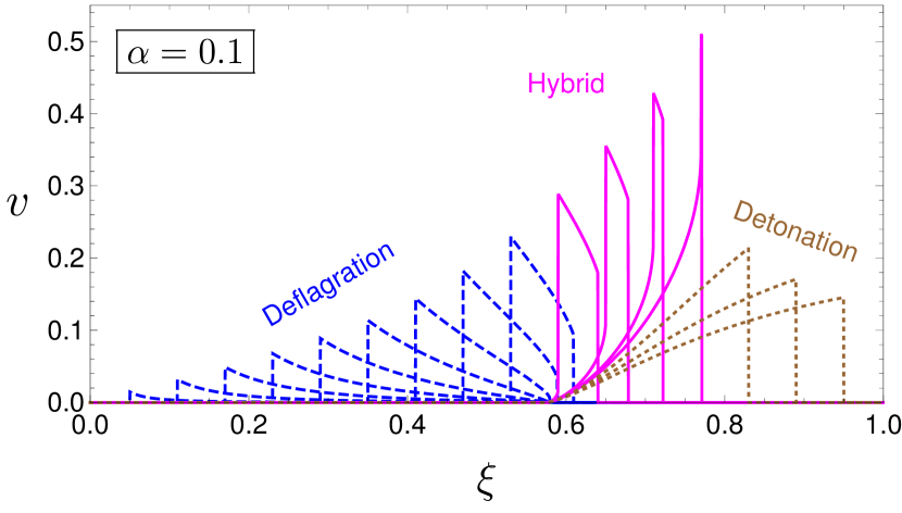
Figure 2: A set of fluid velocity profiles obtained when $v_{w}$ is increased from small to large values(from left to right), for $\alpha=0.1$. Three modes of profiles are obtained, deflagration (blue dashed), supersonic deflagration (aka hybrid, magenta solid) and detonation (brown dotted).

This hydrodynamic treatment hinges on solving the fluid velocity profile $v(r,t)$ around the bubble wall given inputs of $(\alpha,v_{w})$, where $r$ is the distance from the bubble center and $t$ is counted from the onset of the EWPT. Due to the properties of the problem here, $v$ is a function solely of $r/t\equiv\xi$. The differential equation governing the velocity profile is derived from the conservation of the energy momentum tensor describing the fluid and scalar field Espinosa:2010hh :

$$2\frac{v}{\xi}=\frac{1-v\xi}{1-v^{2}}\left[\frac{\mu^{2}}{c_{s}^{2}}-1\right]\partial_{\xi}v,$$ (17)

where $c_{s}=1/\sqrt{3}$ is the speed of sound in the plasma and $\mu(\xi,v)=(\xi-v)/(1-\xi v)$ is a Lorentz boost transformation. Far outside the bubble and deep inside the bubble, the plasma will not be stirred, that is $v\rightarrow 0$ serves as the boundary condition. At the phase boundary, the velocity of the plasma inside and outside the bubble wall are denoted as $v_{-}$ and $v_{+}$ in the bubble wall frame, both heading towards the bubble center. The same energy momentum conservation, when applied across the bubble wall, gives a continuity equation connecting $v_{-}$ with $v_{+}$. Therefore the whole fluid velocity profile can be solved from the center of the bubble to far outside the bubble where the plasma is unstirred.

The solutions of the fluid profiles can be classified into three modes depending on the value of $v_{w}$. A set of profiles $v(\xi)$ are shown in Fig. 2 for $\alpha=0.1$. For $v_{w}<c_{s}$, a deflagration mode is obtained, in which case, the plasma ahead of the bubble wall flows outward while it remains static inside the bubble, corresponding to the profiles with blue-dashed lines. It can also be seen from this figure that as $v_{w}$ increases in this mode, a discontinuity in $v(\xi)$ appears outside the bubble and $v(\xi)$ jumps to zero. This is the location of the shock front, and beyond this point the solution of Eq. 17 is invalid and a shock front develops such that $v(\xi)$ goes to zero consistently. When $v_{w}$ surpasses $c_{s}$ but is less than a certain threshold $\xi_{J}(\alpha)$, a supersonic deflagration mode KurkiSuonio:1995pp appears (magenta solid profiles) where the plasma inside the bubble has a non-zero profile, while still taking the form of deflagration outside the bubble. Here $\xi_{J}(\alpha)$, as a function of $\alpha$, corresponds to the Jouguet detonation Steinhardt:1981ct , used in earlier studies. It is also evident that in this mode, as $v_{w}$ increases, the shock front becomes closer to the bubble wall until it coincides with the bubble wall, where $v_{w}=\xi_{J}(\alpha)$ and the fluid enters the third, detonation mode (brown dotted profiles). In this mode, the plasma outside the bubble has zero velocity and therefore $v_{+}=v_{w}$. If a subsonic velocity is required in EWBG, we conclude that the deflagration mode will not work for EWBG. On the contrary, $v_{+}<v_{w}$ in the deflagration and supersonic deflagration modes and a solution for the tension between EWBG and GW might be achieved.

Therefore, instead of treating $v_{w}$ as a free parameter in the GW calculations, we require, given a certain input of $\alpha$, the corresponding $v_{+}$ to have subsonic value, taken to be $0.05$ here, a choice usually used in EWBG calculations John:2000zq ; Cirigliano:2006dg ; Chung:2009qs ; Chao:2014dpa ; Guo:2016ixx ). The procedure of achieving the above goal is as follows: for each given $\alpha$ we iterate over $v_{w}$ and solve the whole fluid profile until $v_{+}=0.05$ is reached. The resulting $v_{w}$ is used in GW calculations .

With $v(\xi)$ obtained, one can also calculate the bulk kinetic energy normalized by the vacuum energy released during the EWPT Espinosa:2010hh :

$$\kappa_{v}=\frac{3}{\Delta\rho\ v_{w}^{3}}\int\omega(\xi)\frac{v^{2}}{1-v^{2}}\xi^{2}d\xi,$$ (18)

where $\omega(\xi)$ is the enthalpy density, varying as function of $\xi$, and can be solved once $v(\xi)$ is found. The remaining part $1-\kappa_{v}\equiv\kappa_{T}$ gives the fraction of the vacuum energy going to heat the plasma. Therefore a reheating temperature can be defined as

$$T_{\ast}=T_{n}(1+\kappa_{T}\alpha)^{1/4}.$$ (19)

This leads to an increase in entropy density and thus a dilution of the generated baryon asymmetry Patel:2012pi . Typically in EWBG calculations, the wall curvature is neglected and the transport equations depend on a single coordinate $\bar{z}$ in the bubble wall rest frame, where $\bar{z}>0$ ($<0$) corresponds to broken (unbroken) phase. The solved baryon asymmetry density $n_{B}$ is a constant inside the bubbles(see, e.g., Lee:2004we ):

$$n_{B}=\frac{3\Gamma_{\mathrm{ws}}}{D_{q}\lambda_{+}}\int_{0}^{-\infty}n_{L}(\bar{z})e^{-\lambda_{-}\bar{z}}d\bar{z}\ \ ,$$ (20)

where $s(T)=2g_{\ast}\pi^{2}T^{3}/45$ is the entropy density, $\Gamma_{\text{ws}}\approx 120\alpha_{w}^{5}T$ is the weak Sphaleron rate in the EW symmetric phase Bodeker:1999gx , $\lambda_{\pm}=(v_{+}\pm\sqrt{v_{+}^{2}+15\Gamma_{\text{ws}}D_{q}})/(2D_{q})$ with $D_{q}$ the diffusion constant for quarks Bodeker:1999gx and $n_{L}$ is the chiral asymmetry of left-handed doublet fields which serves as a source term in baryon asymmetry generation. The determination of $n_{L}$ is a key part in EWBG calculations and is decoupled from the analysis of EWPT dynamics here. In above expression, we have replaced $v_{w}$ by $v_{+}$, to take into account the distinction between these two velocities. If the temperature at which $n_{B}$ is calculated is $T_{n}$, then after the bubbles have collided, the temperature of the plasma is given, to a good approximation, by $T_{\ast}$ rather than $T_{n}$ or $T_{c}$, which are conventionally used. The diluted baryon asymmetry is then given by

$$\frac{n_{B}}{s}|_{T=T_{\ast}}=\xi_{D}\frac{n_{B}}{s}|_{T=T_{n}},$$ (21)

where $\xi_{D}\equiv(1+\kappa_{T}\alpha)^{-3/4}$ captures the dilution effect of the generated baryon asymmetry by reheating of the plasma. We then need to make sure that $\xi_{D}$ does not become too small, since otherwise a stronger CP-violation will be needed, which might be excluded by the stringent limits from electric dipole moment searches Engel:2013lsa ; Chupp:2017rkp .

4.3 Stochastic Gravitational Waves

During the EWPT, bubbles of EW broken phase expand and collide with each other, which destroys the spherical symmetry of a single bubble, thus leading to the emission of gravitational waves Kamionkowski:1993fg . Due to the nature of this process and according to the central limit theorem, the generated gravitational wave amplitude is a random variable which is isotropic, unpolarized and follows a Gaussian distribution. This therefore allows the description of gravitational wave amplitude using its two-point correlation function and is parametrized by the gravitational wave energy density spectrum $\Omega_{\text{GW}}(f)$, as a function of frequency $f$. A natural consequence is that the GWs produced during the EWPT, when redshifted to the present, give a peak frequency at around the milli-Hertz range Grojean:2006bp , falling right within the band of future space-based gravitational wave detectors.

It is now well known that there are mainly three sources of gravitational wave production in this process: bubble wall collisions Kosowsky:1991ua ; Kosowsky:1992rz ; Kosowsky:1992vn ; Huber:2008hg ; Jinno:2016vai ; Jinno:2017fby , sound waves in the plasma Hindmarsh:2013xza ; Hindmarsh:2015qta and magneto-hydrodynamic turbulence (MHD) Hindmarsh:2013xza ; Hindmarsh:2015qta . The total energy density spectrum can be obtained approximately by adding these contributions:

$$\Omega_{\text{GW}}h^{2}\simeq\Omega_{\text{col}}h^{2}+\Omega_{\text{sw}}h^{2}+\Omega_{\text{turb}}h^{2}.$$ (22)

Recent studies suggest that the energy deposited in the bubble walls is negligible, despite the possibility that the bubble walls can run away in some circumstances Bodeker:2009qy . Therefore while a bubble wall can reach relativistic speed, its contribution to gravitational waves can generally be neglected Bodeker:2017cim . We thus include only the contribution of sound waves and turbulence in the gravitational wave spectrum calculations.

The dominant contribution comes from sound waves. By evolving the scalar-field and fluid model on 3-dimensional lattice, the gravitational wave energy density spectrum can be extracted, with an analytical fit formula available Hindmarsh:2015qta :

$$\Omega_{\textrm{sw}}h^{2}=2.65\times 10^{-6}\left(\frac{H_{\ast}}{\beta}\right)\left(\frac{\kappa_{v}\alpha}{1+\alpha}\right)^{2}\left(\frac{100}{g_{\ast}}\right)^{1/3}$$

$$\hskip 39.83368pt\times v_{w}\left(\frac{f}{f_{\text{sw}}}\right)^{3}\left(\frac{7}{4+3(f/f_{\textrm{sw}})^{2}}\right)^{7/2}\ .$$ (23)

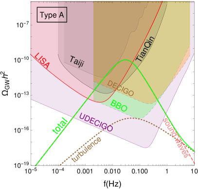
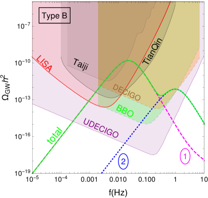
Figure 3: Examples showing GW energy density spectra from one step (left) and two-step (right) EWPT. For the left panel, the individual contributions from sound waves and magnetohydrodynamic turbulence are shown with their sum denoted by the green solid line. For the right panel, the total contributions from both the first step and second step are shown and with their sum denoted by the green solid line.

Here $H_{\ast}$ is the Hubble parameter at $T_{\ast}$ when the phase transition has completed. It has a value close to that evaluated at the nucleation temperature $T_{n}$ for sufficiently short EWPT Caprini:2015zlo . We take $T_{\ast}$ to be the reheating temperature, defined earlier in Eq. 19. Moreover, $f_{\text{sw}}$ is the present peak frequency which is the redshifted value of the peak frequency at the time of EWPT ($=2\beta/(\sqrt{3}v_{w})$):

$$f_{\textrm{sw}}=1.9\times 10^{-5}\frac{1}{v_{w}}\left(\frac{\beta}{H_{\ast}}\right)\left(\frac{T_{\ast}}{100\textrm{GeV}}\right)\left(\frac{g_{\ast}}{100}\right)^{1/6}\textrm{Hz},$$ (24)

where $\kappa_{v}$ is defined in Eq. 18 and can be calculated as a function of ($\alpha$, $v_{w}$) by solving the velocity profiles described in Sec. 4 Espinosa:2010hh . It should be noted that a more recent numerical simulation by the same group Hindmarsh:2017gnf ; Hindmarsh:2016lnk shows a slightly enhanced $\Omega_{\text{sw}}h^{2}$ and reduced peak frequency $f_{\text{sw}}$. We also note that the results from these simulations are currently limited to regions of small $v_{w}$ and $\alpha$ and therefore their validity for ultra-relativistic $v_{w}$ and large $\alpha$ (say $\alpha\gtrsim 1$) remains unknown. In the absence of numerical simulations for these choices of parameters at present, we assume that the results shown here apply for these cases and remind the reader to keep the above caveats in mind.

The fully ionized plasma at the time of EWPT can result in the formation of MHD turbulence, which gives another source of gravitational waves. The resulting contribution can also be modelled similarly with a fit formula Caprini:2009yp ; Binetruy:2012ze ,

$$\Omega_{\textrm{turb}}h^{2}=3.35\times 10^{-4}\left(\frac{H_{\ast}}{\beta}\right)\left(\frac{\kappa_{\text{turb}}\alpha}{1+\alpha}\right)^{3/2}\left(\frac{100}{g_{\ast}}\right)^{1/3}$$

$$\hskip 51.21504pt\times v_{w}\frac{(f/f_{\textrm{turb}})^{3}}{[1+(f/f_{\textrm{turb}})]^{11/3}(1+8\pi f/h_{\ast})},$$ (25)

where $f_{\text{turb}}$ is the peak frequency and is given by,

$$f_{\textrm{turb}}=2.7\times 10^{-5}\frac{1}{v_{w}}\left(\frac{\beta}{H_{\ast}}\right)\left(\frac{T_{\ast}}{100\textrm{GeV}}\right)\left(\frac{g_{\ast}}{100}\right)^{1/6}\textrm{Hz}.$$ (26)

Here the factor $\kappa_{\text{turb}}$ describes the fraction of energy transferred to the MHD turbulence and is given roughly by $\kappa_{\text{turb}}\approx\epsilon\kappa_{v}$ with $\epsilon\approx 5\sim 10\%$ Hindmarsh:2015qta . We take $\epsilon=0.1$ in this study.

In both Eq. 23 and  25, the value of $v_{w}$ is found by requiring that $v_{+}=0.05$ by solving the velocity profiles, as discussed in the previous section. For the two-step EWPT, as discussed in last section, if both steps in case (B) and (C) are first order, then there would be two subsequent GW generation at generally different peak frequencies and amplitudes, corresponding to the example shown in the right panel of Fig. 3.

The detectability of the GWs is quantified by the signal-to-noise ratio (SNR), whose definition is given in Ref. Caprini:2015zlo :

$$\text{SNR}=\sqrt{\delta\times\mathcal{T}\int_{f_{\text{min}}}^{f_{\text{max}}}df\left[\frac{h^{2}\Omega_{\text{GW}}(f)}{h^{2}\Omega_{\text{exp}}(f)}\right]^{2}}.$$ (27)

Here $h^{2}\Omega_{\text{exp}}(f)$ is the experimental sensitivity and corresponds to the lower boundaries of the color-shaded regions in Fig. 3 for the shown detectors . $\mathcal{T}$ is the mission duration in years for each experiment, assumed to be $5$ here. The factor $\delta$ comes from the number of independent channels for cross-correlated detectors, which equals $2$ for BBO as well as UDECIGO and $1$ for the others Thrane:2013oya . In our numerical analysis, we stick to the most mature LISA detector with the C1 configuration, defined in Ref. Caprini:2015zlo . To qualify for detection, the SNR needs to be larger than a threshold value, which depends on the details of the detector configuration. For example, for a four-link LISA configuration, the suggested value is 50 while for a six-link configuration, this value can be much lower ($\text{SNR}=10$), since in this case a special noise reduction technique is available based on the correlations of outputs from the independent sets of interferometers of one detector Caprini:2015zlo .

As an example, we scan over the EW vacuum stability regions in the plane $(v_{s}/v_{\text{EW}},b_{3}/v_{\text{EW}})$ of Fig. 1 and found the regions which can give successful bubble nucleations, satisfy the SFOEWPT criterion and generate GWs. These regions are plotted with blue ($\text{SNR}<10$), green ($50>\text{SNR}>10$) and red ($\text{SNR}>50$). Here most of the points give type (A) EWPT with only several points for type (B) or (C), denoted by diamond shapes.

5 Results and Discussions

In this section, we perform a full scan of the parameter space to address the following questions:

• What kind of EWPT patterns can this model admit and in what proportion of the parameter space for each pattern?

• What is the region of parameter space that can give strong detectable gravitational waves at future space-based gravitational wave detectors?

• Do current collider measurements of double Higgs production and searches for a heavy resonance decaying to weak boson pairs exclude the points that give strong gravitational waves and could future high luminosity LHC (HL-LHC) at $3\text{ab}^{-1}$ probe the parameter space giving strong gravitational waves?

• How will a future space-based gravitational wave experiment complement current and future searches for a heavy scalar resonance?

We find that it is more efficient to cover the parameter space in the scan using the tadpole basis parameters. So we start the random number generating in the tadpole basis. Once a parameter space point is obtained from the sampling, it is converted to the non-tadpole basis parameters and for all subsequent phenomenological checks and calculations. The ranges of the tadpole basis parameters where we do the random sampling are the following:

$$b_{4}\in[0.001,5],\quad\quad b_{3}/v_{\text{EW}}\in[-10,10],\quad$$

$$a_{2}\in[-2\sqrt{\lambda b_{4}},25],\quad\theta\in[-0.35,0.35],$$

$$m_{h_{2}}\in[260,1000],$$ (28)

where the lower range of $a_{2}$ is determined by the requirement that the potential is bounded from below. The scan takes into account the previously discussed theoretical and phenomenological requirements. Points which pass these selection criteria are fed into a modified version of CosmoTransitions Wainwright:2011kj for calculating the thermal history and the parameters relevant for EWPT . Those which can give a successful EWPT by meeting the bubble nucleation criteria are further scrutinized for the EWPT type and SFOEWPT conditions. The final remaining points are used to calculate the gravitational wave spectra, the SNR and collider observables.

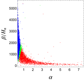
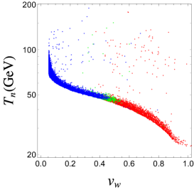
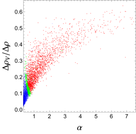
Figure 4: The physical parameters characterizing the dynamics of the EWPT: in the plane of $(\alpha,\beta/H_{n})$ (left), $(v_{w},T_{n})$ (middle) and ($\alpha,\Delta\rho_{V}/\Delta\rho$) (right). In all these plots, the colors denote $\text{SNR}>50$ (red), $50>\text{SNR}>10$ and $\text{SNR}<10$ (blue). Points depicted here pass all phenomenological constraints and give successful bubble nucleations.

5.1 EWPT and GW

We first give the answer to question (a): what kind of EWPT patterns can this model admit and in what proportion of the parameter space for each pattern ?

We find, of the xSM parameter space where a successful EWPT can be obtained, about $99\%$ gives type (A) EWPT and the remaining slightly less than $1\%$ can give type (B) EWPT. We do not observe type (C) EWPT. For type (A), $22\%$ ($19\%$) gives SNR larger than $10$ ($50$). So there is a sufficiently large parameter space which can give detectable GW production.

The strength of the stochastic GW background is mainly governed by the two parameters $\alpha$ and $\beta/H_{n}$, where a larger $\alpha$ and a smaller $\beta/H_{n}$ gives stronger GW SNR, as shown in the left panel of Fig. 4, where the colors denote $\text{SNR}<10$ (blue), $50>\text{SNR}>10$ (green) and $\text{SNR}>50$ (red). We observe that the points which give detectable GWs lie in the bottom right region of the population.

Physically, $\alpha$ quantifies the amount of energy released during the EWPT and therefore a larger $\alpha$ gives stronger GW signals. In addition, for fixed $v_{w}$, a larger $\alpha$ leads to a larger fraction of energy transformed into the plasma kinetic energy, quantified by $\kappa_{v}$, and therefore a further gain in GW production. A further enhancement for larger $\alpha$ comes from the fact that since we fixed $v_{+}=0.05$, increasing $\alpha$ also increases $v_{w}$. It should be noted, even without an explicit calculation, that for each fixed value of $\alpha$, the allowed values of $v_{w}$ are limited to a certain range (see e.g., Fig. 1 in Ref. Alves:2018oct ). This comes from two considerations: (1) admitting consistent hydrodynamic solutions of the plasma imposes a lower limit on $v_{w}$; (2) $v_{w}$ larger than $\xi_{J}(\alpha)$ gives a detonation mode of the velocity profile, in which case $v_{w}=v_{+}>c_{s}$ and therefore $v_{+}$ is too large for EWBG to work. We further note that for $\alpha\gtrsim 1$ and $v_{w}\sim 1$, the calculations of the GW spectra may become unreliable for the following reasons: ($i$) While the study of Ref. Bodeker:2017cim suggests that the energy stored in the scalar field kinetic energy is negligible, a very large $\alpha$ might lead to a non-negligible contribution from the bubble collisions. Therefore a better understanding of the energy budget for this region is needed; ($ii$) the numerical simulations are all performed for relatively small $\alpha$ as well as $v_{w}$ and thus the use of these results for large $\alpha$ and $v_{w}$ may not be applicable; ($iii$) The universe is no longer radiation dominated at the EWPT but rather vacuum energy dominated. This has the consequence that bubbles might never meet to finish the EWPT and the universe would be trapped in the metastable phase (see Ref. Ellis:2018mja for a recent analysis). Despite these issues, we find $49\%$ of points with $\text{SNR}>10$ have $\alpha<1$ and removing the points with $\alpha>1$ does not change the main findings of our work.

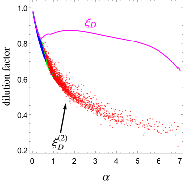
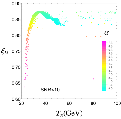
Figure 5: Figures showing the dilution effect of the baryon asymmetry. The left panel shows two different definitions of the dilution factor and the right panel shows the dilution factor $\xi_{D}$ defined in Eq. 21 versus $T_{n}$.

We now turn to the parameter $\beta/H_{n}$, which roughly characterizes the inverse time duration of the EWPT. A smaller $\beta/H_{n}$ or equivalently a longer EWPT generates stronger GW signals. This is due to the particular feature of the GWs coming from the sound waves in the plasma. As was found in the original papers on the importance of sound waves in generating the GWs Hindmarsh:2013xza ; Hindmarsh:2015qta , one enhancement comes from $1/(\beta/H_{n})$ compared with the conventional bubble collision contribution. As long as the mean square fluid velocity of the plasma is non-negligible, GWs will continue being generated and the energy density of the GW is thus proportional to the duration of the EWPT. It should be noted that $\beta/H_{n}$ also determines the peak frequency of the GW spectra.

The bubble wall velocity $v_{w}$ also plays an important role here and the dependence of the SNR on $v_{w}$ is shown in the middle panel of Fig. 4, where the vertical axis is chosen to be $T_{n}$. It is clear that points with larger SNR have larger $v_{w}$ since, for fixed $v_{+}$, a larger $\alpha$ implies a larger $v_{w}$. It can also be seen from this plot that the SNR increases as $T_{n}$ decreases. This is easily understood, since a smaller $T_{n}$ typically implies a larger amount of supercooling and therefore a larger $\alpha$. The supercooling can be quantified by the fraction of the first term($\equiv\Delta\rho_{V}$) of Eq. 15 in the total released vacuum energy, which we plot in the right panel. We can see from this figure that larger SNR indeed implies larger amount of supercooling. However the amount of supercooling as quantified by $\Delta\rho_{V}/\Delta\rho$ is less than $0.6$ for most of the parameter space. The remaining part comes from the second term of the definition of $\alpha$.

The entropy production, if sizeable, can pose a problem for baryon asymmetry generation, as it will effectively dilute the baryon asymmetry $n_{B}/s$ by increasing $s$. In Sec. 4.2, we encode this effect in a dilution factor $\xi_{D}$. Here since $\kappa_{T}$ is a function of $v_{w}$ and $\alpha$ while $v_{w}$ is also a function of $\alpha$ when $v_{+}$ is fixed, we find $\xi_{D}$ is solely a function of $\alpha$. This functional relation is shown as the magenta line in the left panel of Fig. 5 and all points from the scan fall on this line. The message from this figure is that most of the points have $\xi_{D}\gtrsim 0.65$ and those with a smaller $\alpha$ have a dilution factor closer to $1$. In particular, the points with $\alpha\lesssim 1$ for which GW can be reliably calculated, the dilution effect is rather small as $\xi_{D}\gtrsim 0.8$. Given the current relatively large uncertainties in the EWBG calculations, the dilution effect poses no real problem for the baryon asymmetry generation. Note that previous studies Patel:2012pi used a different quantification of the dilution factor, with the definition:

$$\xi_{D}^{(2)}=\frac{s}{s+\Delta s},$$ (29)

where $s$ is the entropy density at $T_{n}$ and $\Delta s$ is calculated from the second term in the definition of $\alpha$ in Eq. 15. To compare with the factor $\xi_{D}$, what we use here, we show values of this factor in the same plot of $\xi_{D}$ for every point that gives detectable GWs. It is evident from this figure that these two factors are roughly the same and both decrease linearly for $\alpha\lesssim 0.4$. For $\alpha\gtrsim 0.4$, $\xi_{D}^{(2)}$ gives an overestimation of the dilution effect while $\xi_{D}$ firstly increases a little bit before slowly dropping. Since the dilution factor we use here is based on a faithful hydrodynamic analysis, it gives a more precise description of the dilution effect. We also show $\xi_{D}$ calculated for all the points versus $T_{n}$ as a scatter plot in the right panel of Fig. 5, from which we find a larger dilution effect appears for typically smaller $T_{n}$ and those with $\alpha\lesssim 1$ fall in the high $T_{n}$ region.

The two-step EWPT, for which type (B) is the only observed here, constitutes about one percent of all the surviving parameter space. Of this tiny parameter space, more than half the points give detectable GWs.

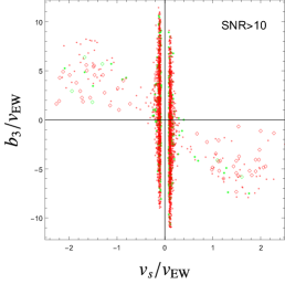
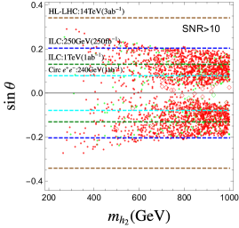
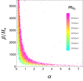
Figure 6: Points depicted here pass all phenomenological constraints and give successful bubble nucleations, along with detectable GWs at LISA ($\text{SNR}>10$). We show them in the planes of the input parameters: in plane $(b_{3},v_{s})/v_{\text{EW}}$ (left) and $(\sin\theta,m_{h_{2}})$ (middle). We distinguish those points which give $\text{SNR}>50$ (red) with those of $50>\text{SNR}>10$ (green) in these two plots. The right panel shows all the points in the plane $(\alpha,\beta/H_{n})$ with the colors denoting the values of $m_{h_{2}}$, as shown in the legend.

5.2 Parameter Space Giving Detectable GWs

With a summary of the points described in previous section, we give in this section the answer to question (b), which, we recall, was: What is the region of parameter space that can give strong detectable gravitational waves at future space-based gravitational wave detectors?

The results are shown in terms of the three plots in Fig. 6. As was discussed in the previous section, a large $\alpha$ and small $\beta/H_{n}$ leads to loud GW signals. Even though the relation between $(\alpha,\beta/H_{n})$ and the physical input parameters is not transparent as many numerical details are involved, it can still be revealed by the plots in Fig. 6. From the left panel in Fig. 6, we can see that the majority of the points are concentrated in two regions of parameter space where $v_{s}$ is rather small. In particular, we find $20\,\text{GeV}\lesssim|v_{s}|\lesssim 50\,\text{GeV}$ for most points, with a peak distribution at around $20\,\text{GeV}$. The appearance of two regions comes from the bounded-from-below requirement of the potential, similar to Fig. 1. While phenomenological constraints have the effect of shrinking both the regions, the appearance of points far outside the two regions indeed shows that the main cause of the narrow regions comes from the requirements of EWPT and GWs. Therefore it is fair to say that the region that gives detectable GWs from a type (A) EWPT mainly comes from the parameter space with smaller $v_{s}$. On the other hand, the regions which provide type (B) EWPT are dramatically different from these regions, since most of the diamonds lie beyond the two narrow regions, as can be seen from the figure.

The middle figure shows these regions in the $(m_{h_{2}},\sin\theta)$ plane. It is clear that the points are concentrated around the region with larger $m_{h_{2}}$. For smaller $m_{h_{2}}$, the density of points becomes much smaller. To have a better understanding of the role of $m_{h_{2}}$ in GW production, we show in the right panel its role in determining $(\alpha,\beta/H_{n})$, denoted by the colors. In this figure, the points are separated into different bands characterized by the value of $m_{h_{2}}$. For fixed $\beta/H_{n}$, a larger $m_{h_{2}}$ gives a larger $\alpha$, thus larger SNR. This explains the concentration of the points in the $m_{h_{2}}$ direction in the middle figure. In the $\sin\theta$ direction, the value of $\theta$ is more constrained for larger $m_{h_{2}}$. The outer boundary comes mainly from the $W$-mass constraint. The requirements from EWPT and larger GW signals also show their effects in this plot. For example, very small values of $\theta$ give rarer points. We also overlaid on this plot the various sensitivity projections from colliders in probing the value of $\theta$, which includes HL-LHC, ILC with two configurations (ILC-1: $250\text{GeV}$, $250\text{fb}^{-1}$, ILC-3: $1\text{TeV}$,$1\text{ab}^{-1}$) and future circular $e^{+}e^{-}$ colliders ($240\text{GeV},1\text{ab}^{-1}$), all taken from Ref. Profumo:2014opa . We see that HL-LHC can barely probe any points; ILC-1 can probe a fraction of the small $m_{h_{2}}$ points as well as a few large $m_{h_{2}}$ points; ILC-3 can probe about a half of both light and heavy $h_{2}$ points; the future circular colliders can probe even more of the parameter space. We also can see that most of the points coming from the two-step EWPT lie at the very small $\theta$ region, even though a few do have larger $\theta$. Therefore GW detections serve as a complementary probe of this region. We also note that for very small values of $\theta$ and $m_{h_{2}}$, the search for long lived particles can be used to probe this region (eg., the MATHUSLA detector) Curtin:2018mvb .

5.3 Correlation with Double Higgs Production Searches

Exploring possible deviations from the expected SM value of the cubic Higgs coupling through di-Higgs production is an important target of the HL-LHC. New physics scenarios, especially those designed for providing a SFOEWPT for baryon asymmetry generation, typically modify this coupling. Therefore di-Higgs production is correlated with EWPT and thus GW production. Future GW and collider experiments can then operate in a way that complement each other in exploring new physics scenarios. With the parameter space giving detectable GW identified in the previous section, we can find the correlation by calculating the corresponding di-Higgs cross sections and compare it with present di-Higgs measurements and with future projections.

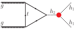
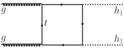
Figure 7: Representative resonant (left) and non-resonant (middle and right) Feynman diagrams contributing to di-Higgs production.

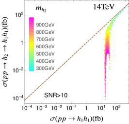
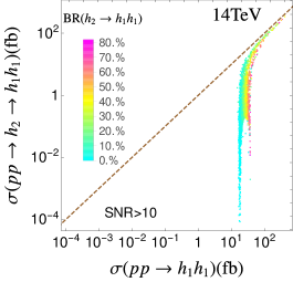
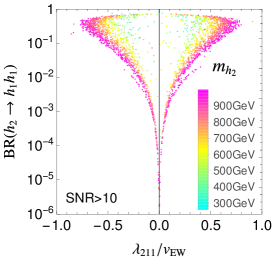
Figure 8: Resonant contribution to the cross section for di-Higgs production, versus the total cross-section. The left plot shows the correlation of the two cross sections, with the colors denoting values of $m_{h_{2}}$. The middle plot has the colors switched to the branching ratio of $h_{2}\rightarrow h_{1}h_{1}$. The right plot shows this branching ratio versus the trilinear coupling $h_{2}h_{1}h_{1}$, where the color denotes $m_{h_{2}}$. In the left two plots, the dashed line denotes the place where these two cross sections are the same.

The leading order Feynman diagrams for double Higgs production occur at one-loop and consist of both the resonant and non-resonant channels, as shown in Fig. 7. The non-resonant channel includes the box diagrams and a triangle diagram involving the vertex $h_{1}h_{1}h_{1}$. The resonant channel is the production of a on-shell $h_{2}$ which subsequently decays into two Higgs, thus including the $h_{2}h_{1}h_{1}$ vertex. The amplitude at leading order was given in the early papers Eboli:1987dy ; Plehn:1996wb with the result expressed in terms of Passarino-Veltman scalar integrals. This result has also been implemented into MadGraph Alwall:2014hca taking into account the presence of a heavier SM-like scalar , which we use for calculating the corresponding cross sections for each point shown here. This takes as input the modified Higgs top Yukawa coupling, the Higgs trilinear coupling, the heavy scalar top coupling, the $h_{2}h_{1}h_{1}$ coupling and the mass as well as the decay width of $h_{2}$. Since $h_{2}$ decays into SM particles with reduced coupling $(-\sin\theta)$ as compared with the SM Higgs and also decays to a pair of $h_{1}$, the total width is simply given by:

$$\Gamma_{h_{2}}=\sin^{2}\theta\,\Gamma_{\text{SM}}(h_{2}\rightarrow X_{SM})+\Gamma(h_{2}\rightarrow h_{1}h_{1}),$$ (30)

where $\Gamma_{\text{SM}}(h_{2}\rightarrow X_{SM})$ denotes an exact SM Higgs-like $h_{2}$ decaying into the SM particles.

For the di-Higgs production, if the resonant production of $h_{1}h_{1}$ via the $h_{2}$ resonance dominates the cross section, then the cross section can be written in the narrow width approximation as

$$\sigma(pp\rightarrow h_{1}h_{1})=\sigma(pp\rightarrow h_{2})\text{BR}(h_{2}\rightarrow h_{1}h_{1}).$$ (31)

In reality, interference effects between the resonant and non-resonant diagrams may be important and lead to constructive or destructive effect on the final full cross section Carena:2018vpt . We thus compare, for each scanned point, the obtained cross section for both the full calculation and the above approximation from the purely resonant production. This is shown in the left and middle plots of Fig. 8 for $\sigma(pp\rightarrow h_{1}h_{1})$ versus $\sigma(pp\rightarrow h_{2}\rightarrow h_{1}h_{1})$ for all the points which give detectable GW signals, that is, those with $\text{SNR}>10$. These cross sections are both calculated at leading order but we have added a common K-factor of $2.27$ deFlorian:2013uza to take into account of higher order corrections. The colors in the left panel denote the values of $m_{h_{2}}$ and those in the middle denote $\text{BR}(h_{2}\rightarrow h_{1}h_{1})$. It is clear from these figures that the resonant cross section is always less than the full one-loop result and drops sharply as $m_{h_{2}}$ is increased (left panel). Since, as we have seen in previous sections, the points with large SNR are concentrated around the region with larger $m_{h_{2}}$, most of the points with detectable GWs turn out to give small di-Higgs production and even negligible resonant production. The colors in the left panels make it clear that most of the points which have larger $m_{h_{2}}$ (and larger SNR) tend to give very small di-Higgs production, with a cross section of $\mathcal{O}(10)\text{fb}$, while smaller $m_{h_{2}}$ gives $\mathcal{O}(100)\text{fb}$. Moreover, there is a sharp drop of the resonant production cross section. From the middle panel, we can see that the color of decreasing branching ratio $h_{2}\rightarrow h_{1}h_{1}$ coincides partly with increasing $m_{h_{2}}$ for the very large $m_{h_{2}}$ points. The small branching ratio is found for a majority of points and is due to the smallness of $\lambda_{211}$. This can be seen from the right panel, where this correlation is shown with the color denoting $m_{h_{2}}$. It is found that a majority of points which have large $m_{h_{2}}$ give small branching ratio. This can partly explain the cause of the drop of the resonant production.

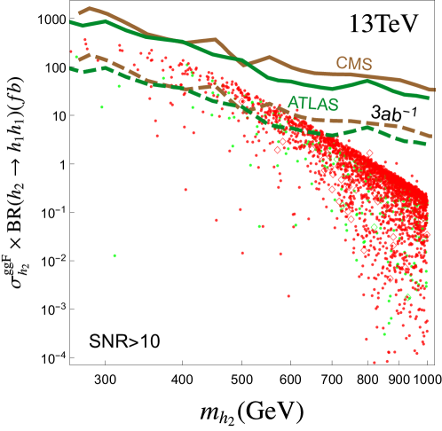
Figure 9: The upper limits on di-Higgs resonant production cross section from ATLAS and CMS combined searches, shown as solid green and brown lines for ATLAS and CMS, respectively. The dashed lines denote the corresponding future projections for $3\text{ab}^{-1}$ of data at the HL-LHC (13TeV). As in the other plots, we distinguish those points which give SNR $>$ 50 (red) and those of 50 $>$ SNR $>$ 10 (green).

On the experimental side, both the ATLAS and CMS collaborations have recently published their search results for non-resonant and resonant di-Higgs productions using the data collected in 2016 at 13 TeV, with nearly the same integrated luminosity. The CMS search result is based on the $35.9\text{fb}^{-1}$ data, in the di-Higgs decay channels $b\bar{b}\gamma\gamma$ Sirunyan:2018iwt , $b\bar{b}\tau^{+}\tau^{-}$ Sirunyan:2017djm , $b\bar{b}b\bar{b}$ Sirunyan:2017isc ; Sirunyan:2018zkk ; Sirunyan:2018qca ; Sirunyan:2018tki and $b\bar{b}WW/ZZ$ Sirunyan:2017guj , with a recent combination given in Sirunyan:2018two . ATLAS used $36.1\text{fb}^{-1}$ data and searched in channels $\gamma\gamma b\bar{b}$ Aaboud:2018ftw , $b\bar{b}\tau^{+}\tau^{-}$ Aaboud:2018sfw , $b\bar{b}b\bar{b}$ Aaboud:2018knk , $WW^{(\ast)}WW^{(\ast)}$ Aaboud:2018ksn and $b\bar{b}WW^{\ast}$ Aaboud:2018zhh , with also a combination of the first three channels ATLAS:2018otd . We use the ATLAS and CMS combined limits in the resonant production channels and show them with green and brown solid lines respectively in Fig. 9. For the points giving detectable GWs, we calculate the resonant cross sections from gluon fusion at NNLO+NNLL using the available result in Ref. deFlorian:2016spz . We can see that none of the points with detectable GW gives cross section above this limit. With the anticipation of HL-LHC at a luminosity of $3\text{ab}^{-1}$ ($13\text{TeV}$), we can get the future projections of this limit by a simple rescaling and obtain the two dashed lines. For this projection, the region with lower $m_{h_{2}}\lesssim 550\text{GeV}$ can be partly explored by CMS and a little bit higher for ATLAS, while the high mass region remains out of reach for di-Higgs searches. Yet, Some points of the scanned parameters space with observable SNR show a promising di-Higgs production cross section of 50 fb or more at the LHC which, in principle, can be probed with 3 ab^-1. Therefore GW measurements can complement collider searches by revealing the high $m_{h_{2}}$ region of the xSM model.

5.4 Higgs Cubic and Quartic Couplings

Future precise measurements of the Higgs cubic and quartic self-couplings can be used to reconstruct the Higgs potential to confirm ultimately the mechanism of EW symmetry breaking and shed light on the nature of the EWPT. The measurements of above double Higgs production can be used to determine the cubic coupling and there have been extensive studies on this topic DiVita:2017vrr ; Adhikary:2017jtu ; Banerjee:2018yxy . The best sensitivities obtained for these future colliders is typically at $\mathcal{O}(1)$. Despite the more formidable challenges with the quartic coupling measurement, there is now growing interest in it. Several different methods have been proposed and studied: through triple Higgs production measurement Plehn:2005nk , through double Higgs production at hadron colliders where the quartic coupling enters $gg\rightarrow hh$ at two-loop Bizon:2018syu or renormalizes the cubic coupling, and at lepton colliders(via Z-associated production $e^{+}e^{-}\rightarrow Zhh$ and VBF production $e^{+}e^{-}\rightarrow\nu\nu hh$), where the quartic coupling is involved in the $VVhh$ coupling at one loop Liu:2018peg . For example, Ref. Liu:2018peg found a precision of measurement of $\sim\pm 25$ for ($500\text{GeV},4\text{ab}^{-1}$ + 1 TeV, $2.5\text{ab}^{-1}$) and $\sim\pm 20$ for ($500\text{GeV},4\text{ab}^{-1}$ + 1 TeV, $8\text{ab}^{-1}$) at $1\sigma\text{C.L.}$, when the cubic coupling is marginalized in their $\chi^{2}$ analysis.

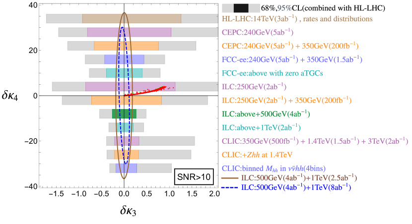
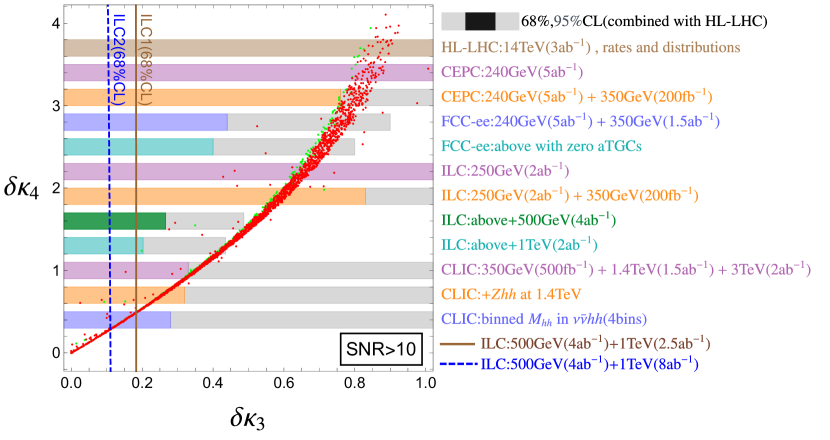
Figure 10: The Higgs cubic and quartic couplings $(\Delta\kappa_{3},\Delta\kappa_{4})$ for parameter space points giving detectable GW. Here the green points give $\text{SNR}>10$ and the red gives $\text{SNR}>50$. The bars denote the sensitivity of $\Delta\kappa_{3}$ from a global analysis of future colliders in Ref. DiVita:2017vrr , for various detector scenarios shown on the right side of the figures. The brown solid and blue dashed lines are the $1\sigma$ contours for two different ILC scenarios taken from Ref. Liu:2018peg . The bottom panel is a zoomed-in version of the top one.

In the xSM, both the Higgs cubic and quartic couplings are modified compared with their SM counterparts:

$$i\lambda_{h_{1}h_{1}h_{1}}=6\Big{[}\lambda vc_{\theta}^{3}+\frac{1}{4}c_{\theta}^{2}s_{\theta}\left(2a_{2}v_{s}+a_{1}\right)+\frac{1}{2}a_{2}vc_{\theta}s_{\theta}^{2}$$

$$\hskip 45.52458pt+\frac{1}{3}s_{\theta}^{3}\left(3b_{4}v_{s}+b_{3}\right)\Big{]},$$ (32)

$$i\lambda_{h_{1}h_{1}h_{1}h_{1}}=6(\lambda c_{\theta}^{4}+a_{2}s_{\theta}^{2}c_{\theta}^{2}+b_{4}s_{\theta}^{4}).$$ (33)

In the absence of mixing of the scalars($\theta=0$), these couplings reduce to the corresponding SM values $i\lambda_{h_{1}h_{1}h_{1}}=3m_{h_{1}}^{2}/v$ and $i\lambda_{h_{1}h_{1}h_{1}h_{1}}=3m_{h_{1}}^{2}/v^{2}$. When $\theta\neq 0$, we parametrize the deviations of these couplings from the SM values as:

$$\Delta\mathcal{L}=-\frac{1}{2}\frac{m_{h_{1}}^{2}}{v}(1+\delta\kappa_{3})h_{1}^{3}-\frac{1}{8}\frac{m_{h_{1}}^{2}}{v^{2}}(1+\delta\kappa_{4})h_{1}^{4},$$ (34)

and show in Fig. 10 these values for the points that give detectable GWs. The features that we can read from this figure are:(1) both $\delta\kappa_{3}$ and $\delta\kappa_{4}$ are positive; (2) both variations are $\mathcal{O}(1)$ as $\delta\kappa_{3}\in(0,1)$ and $\delta\kappa_{4}\in(0,4)$; (3) a correlation exists $\delta\kappa_{4}\equiv\eta\delta\kappa_{3}$, with $\eta\approx 2.8$ for $\delta\kappa_{3}\lesssim 0.4$ and most points fall within $\eta\in(2,4)$. To understand these, we note, since phenomenological constraints requires a small $\theta$, we expect the second feature to follow naturally. The other features can be understood by Taylor expanding the couplings for small $\theta$ and we find:

$$\delta\kappa_{3}=\theta^{2}\left[-\frac{3}{2}+\frac{2m_{h_{2}}^{2}-2b_{3}v_{s}-4b_{4}v_{s}^{2}}{m_{h_{1}}^{2}}\right]+\mathcal{O}(\theta^{3}),$$

$$\delta\kappa_{4}=\theta^{2}\left[-3+\frac{5m_{h_{2}}^{2}-4b_{3}v_{s}-8b_{4}v_{s}^{2}}{m_{h_{1}}^{2}}\right]+\mathcal{O}(\theta^{3}).\quad$$ (35)

In the above square brackets, the terms proportional to $m_{h_{2}}^{2}/m_{h_{1}}^{2}$ dominate for the majority of the points since $v_{s}$ is concentrated at small values; $b_{3}$ is at most $\sim 10v_{\text{EW}}$, $b_{4}\lesssim 5$ from the scan and $m_{h_{2}}\gtrsim 500\text{GeV}$ generally holds. Then the above approximations show positive $\delta\kappa_{3}$ and $\delta\kappa_{4}$ and give $\delta\kappa_{4}/\delta\kappa_{3}\approx 2.5$, which is fairly close to $\eta=2.8$. For relatively large $\theta$, high order corrections need to be taken into account and above linear correlation would be changed.

To compare with the direct measurements of these couplings at future $e^{+}e^{-}$ colliders and the HL-LHC, we added in Fig. 10 the precisions of these measurements from studies in the literature. The two elliptical $68\%$CL closed contours are taken from Ref. Liu:2018peg which focuses on the quartic coupling, for two possible scenarios of the ILC. The bars are the precisions that can be reached from various considerations of future colliders, labelled on the right of the figure, taken from Ref. DiVita:2017vrr (for other studies, see e.g. Borowka:2018pxx ; Bizon:2018syu ; Kilian:2018bhs ; Jurciukonis:2018skr ; Borowka:2018pxx ; Maltoni:2018ttu ; Adhikary:2017jtu ; Banerjee:2018yxy ). Here the inner and outer bar regions denote the $68\%$CL and $95\%$CL results. We can see, it is generically very hard for colliders to probe the cubic coupling at a precision that can reveal the points giving detectable GWs with high confidence level(say 95%) . The most precise comes from the ILC when all possible runs at different luminosities are combined and with the data of HL-ILC included, which gives $0.4\sim 0.5$ uncertainty on the measurement of $\delta\kappa_{3}$ at $95\%$CL. While the analysis in Ref. DiVita:2017vrr does not include the quartic coupling, the contours from Ref. Liu:2018peg do give a hint on its measurement and show that it is infeasible for the colliders to probe the parameter space giving detectable GWs. For the trilinear and quartic coupling deviations that we found, the impact on the triple Higgs cross section is mild for hadron colliders even for a future $pp$ collider at 100 TeV Plehn:2005nk ; Binoth:2006ym , however, resonant contributions in xSM might enhance the cross section up to a factor of ${\cal O}(10)$ Chen:2015gva .

Therefore we expect future GW measurements can make a valuable complementary role in determining the Higgs self-couplings, especially the quartic coupling. While we do not have a statistical analysis here, Fig. 10 does tell us that $\delta\kappa_{4}$ is equally important as $\delta\kappa_{3}$ on GW signal generation since $\eta$ is at most $4$. Thus we expect a full statistical analysis would yield roughly the same precision on the determination of $\delta\kappa_{3}$ and $\delta\kappa_{4}$, which is well improved compared with the situation at colliders.

Figure 11: The branching ratios of $h_{2}$ in $h_{1}h_{1}$ and $VV$ final states, where $VV=WW,ZZ,WW+ZZ$, with the color denoting the value of $m_{h_{2}}$.

5.5 Diboson Resonance Search Limits at Colliders

The $WW$ and $ZZ$ branching ratios become sizeable in parts of the parameter space where the trilinear coupling $\lambda_{211}$ is relatively small, as one can see from the rightmost panel of Fig. 8. In Fig. 11, we show the branching ratios of the $h_{2}\rightarrow WW,ZZ$ and $h_{2}\rightarrow h_{1}h_{1}$ channels. We see that the $WW,ZZ$ channels can be as big as 90% for a large range of $h_{2}$ masses which could show up at searches for weak diboson resonances. Combined, $WW,ZZ$ and $h_{1}h_{1}$ correspond to nearly all the decays of $h_{2}$, which make them the best search channels for $h_{2}$ resonances at colliders.

Besides the di-Higgs production measurements, which can be used to extract the Higgs cubic and quartic couplings, there also exist generic scalar resonance searches at the LHC. In particular, ATLAS and CMS have performed extensive analyses in the searches for a heavier SM-like scalar resonance in $VV$ and $VH$ decay channels of the heavy scalar ($V=W/Z$). ATLAS gives a recent combination of all previous analyses in bosonic and leptonic final states at $\sqrt{s}=13\text{TeV}$ with $36\text{fb}^{-1}$ data collected in 2015 and 2016 Aaboud:2018bun . The limits are drawn for $h_{2}$ production cross section in gluon fusion and vector boson fusion production channels. These two limits are shown in the left and right panels, respectively, in Fig. 12 with green solid lines, together with the detectable GW points. For cross section calculations, we use the set of result calculated to NNLO precision for VBF and for gluon fusion, we use NNLO+NNLL, as also used before in Fig. 9.

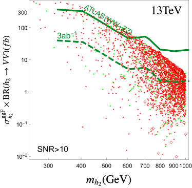
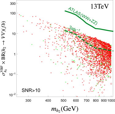
Figure 12: Combined limits from ATLAS (solid line) and future HL-LHC projections (dashed line) for searches of a heavy SM-like resonance in the $WW/ZZ$ channel from gluon fusion (left) and vector boson fusion production (right). As in the other plots, we distinguish those points which give SNR $>$ 50(red) and those of 50 $>$ SNR $>$ 10(green).

It is evident that the current limits from diboson searches are rather loose as most points fall under this line, with gluon fusion limit being able to touch a fraction of the lighter $h_{2}$ point. For the HL-LHC with $\sim 3\text{ab}^{-1}$, we obtain estimates of future projections by a simple scaling factor and obtain the dashed lines for $\sim 3\text{ab}^{-1}$ at $13\text{TeV}$ (while HL-LHC would probably run at $14\text{TeV}$). We can see in all cases that the HL-LHC will probe a larger fraction of the parameter space for both ggH and VBF channels. For ggH, this region covers a range from low to high masses. For VBF, it can cover a region of relatively heavy $h_{2}$. Both channels are sensitive to $h_{1}h_{1}$ cross section times branching ratio down to $\sim 1$ fb in some favorable points of the parameters space. The points that can be probed by HL-LHC serve as promising targets for both colliders and GW detectors but a majority of the parameter space will probably be left to GW detectors.

6 Summary

In this paper, we embarked on a study of the singlet-extended SM Higgs sector. A detailed scan of the parameter space of this model was performed, incorporating all relevant phenomenological constraints, and regions with large SNR at LISA were identified. Subtle issues pertaining to the bubble wall velocity were discussed, and a range of velocity profiles described.

Our main findings are the following. For the parameter space that satisfies all phenomenological constraints, gives successful EWPT and generates GWs, $99\%$ leads to a one-step EWPT with the remaining to two-step EWPT and $22\%$ generates detectable GWs($\text{SNR}>10$) at LISA. The main features of the parameter space that gives detectable GWs is: $20\text{GeV}\lesssim|v_{s}|\lesssim 50\text{GeV}$, where $v_{s}$ is the vev of the singlet field; it is more concentrated in the large $m_{h_{2}}$ region, where $m_{h_{2}}$ is the mass of the heavier scalar $h_{2}$; $\theta\lesssim 0.2$ for the majority of the space. Di-Higgs searches at both ATLAS and CMS are currently unable to probe this parameter space, but HL-LHC will be able to probe the lighter $h_{2}$ region while the heavier $h_{2}$ region will remain elusive. Weak diboson resonance searches cannot constrain xSM much either but the HL-LHC will be able to probe a large fraction of its parameters space in this channel. The Higgs cubic and quartic couplings are at $\mathcal{O}(1)$ deviations from the SM values and obey a relation $\delta\kappa_{4}\approx(2-4)\delta\kappa_{3}$, where $\delta\kappa_{4}$ and $\delta\kappa_{3}$ are the relative deviations of the quartic and cubic couplings from their SM counterparts respectively.

Our results broadly indicate that high energy colliders and GW detectors are going to play complementary roles in probing the parameter space of scalar sectors. Several future directions can be contemplated. It would be interesting to understand how this complementarity plays out in two Higgs doublet models, as well as other scalar sector extensions classified in Chung:2012vg . It would also be interesting to investigate the complementarity of GW and collider probes for phase transitions in the dark sector. We leave these questions for future study.

7 Acknowledgments

A. Alves thanks Conselho Nacional de Desenvolvimento Científico (CNPq) for its financial support, grant 307265/2017-0. K. Sinha is supported by the U. S. Department of Energy grant desc0009956. T. Ghosh is supported by U. S. Department of Energy grant de-sc0010504. We would like to thank David Curtin, Ian Lewis, Hao-Lin Li and Ligong Bian for helpful discussions. We also thank Yi-Ming Hu and Zheng-Cheng Liang of the Tianqin program for sending us the Tianqin sensitivity curve and for valuable discussions.

Appendix A Perturbative Unitarity S Matrix

We consider a total of eleven $2\rightarrow 2$ channels of scalars and longitudinal gauge bosons scatterings. These are grouped into seven charge neutral channels $(h_{1}h_{1},h_{2}h_{2},h_{1}h_{2},h_{1}Z,h_{2}Z,ZZ,W^{+}W^{-})$, three charge-1 channels $(h_{1}W^{+},h_{2}W^{+},ZW^{+})$ and one charge-2 channel $(W^{+}W^{-})$. The leading partial wave amplitudes of these scatterings are given collectively by a symmetric matrix, which itself is a direct sum of the matrices from these three groups: $\mathcal{S}=\mathcal{S}_{0}\bigoplus\mathcal{S}_{1}\bigoplus\mathcal{S}_{2}$. The tree level perturbative unitarity requires that the absolute value of each eigenvalue of this matrix is less than $(1/2\times 16\pi)$. The non-zero elements of the $7\times 7$ matrix $\mathcal{S}_{0}$ is listed as follows(see e.g., Ref. Kanemura:2015ska for a detailed calculation):

$$\mathcal{S}_{11}=-3\left(a_{2}c_{\theta}^{2}s_{\theta}^{2}+b_{4}s_{\theta}^{4}+\lambda c_{\theta}^{4}\right),$$

$$\mathcal{S}_{12}=\frac{1}{8}\left(3\cos(4\theta)\left(-a_{2}+b_{4}+\lambda\right)-a_{2}-3b_{4}-3\lambda\right),$$

$$\mathcal{S}_{13}=\frac{3\sin(2\theta)\left(\cos(2\theta)\left(-a_{2}+b_{4}+\lambda\right)-b_{4}+\lambda\right)}{2\sqrt{2}},$$

$$\mathcal{S}_{16}=-\frac{1}{2}a_{2}s_{\theta}^{2}-\lambda c_{\theta}^{2},$$

$$\mathcal{S}_{17}=-\frac{a_{2}s_{\theta}^{2}+2\lambda c_{\theta}^{2}}{\sqrt{2}},$$

$$\mathcal{S}_{22}=-3\left(a_{2}c_{\theta}^{2}s_{\theta}^{2}+b_{4}c_{\theta}^{4}+\lambda s_{\theta}^{4}\right),$$

$$\mathcal{S}_{23}=-\frac{3\sin(2\theta)\left(\cos(2\theta)\left(-a_{2}+b_{4}+\lambda\right)+b_{4}-\lambda\right)}{2\sqrt{2}},$$

$$\mathcal{S}_{26}=-\frac{1}{2}a_{2}c_{\theta}^{2}-\lambda s_{\theta}^{2},$$

$$\mathcal{S}_{27}=-\frac{a_{2}c_{\theta}^{2}+2\lambda s_{\theta}^{2}}{\sqrt{2}},$$

$$\mathcal{S}_{33}=\frac{1}{4}\left(3\cos(4\theta)\left(-a_{2}+b_{4}+\lambda\right)-a_{2}-3b_{4}-3\lambda\right),$$

$$\mathcal{S}_{36}=\frac{\left(2\lambda-a_{2}\right)c_{\theta}s_{\theta}}{\sqrt{2}},$$

$$\mathcal{S}_{37}=\left(2\lambda-a_{2}\right)c_{\theta}s_{\theta},$$

$$\mathcal{S}_{44}=-a_{2}s_{\theta}^{2}-2\lambda c_{\theta}^{2},$$

$$\mathcal{S}_{45}=\left(2\lambda-a_{2}\right)c_{\theta}s_{\theta},$$

$$\mathcal{S}_{55}=-a_{2}c_{\theta}^{2}-2\lambda s_{\theta}^{2},$$

$$\mathcal{S}_{66}=-3\lambda,$$

$$\mathcal{S}_{67}=-\sqrt{2}\lambda,$$

$$\mathcal{S}_{77}=-4\lambda.$$ (36)

For charge-1 channels, we have:

$$\mathcal{S}_{1}=\left[\begin{array}[]{ccc}-2\lambda c_{\theta}^{2}-a_{2}s_{\theta}^{2}&\left(2\lambda-a_{2}\right)c_{\theta}s_{\theta}&0\\ \left(2\lambda-a_{2}\right)c_{\theta}s_{\theta}&-a_{2}c_{\theta}^{2}-2\lambda s_{\theta}^{2}&0\\ 0&0&-2\lambda\\ \end{array}\right].$$

For the charge-2 channel with only one process, the matrix is simply given by $\mathcal{S}_{2}=(-2\lambda)$.

Appendix B Connection with Potential where $v_{s}=0$

The potential in Eq. 1 can be written into a different form by translating the coordinate system of $(H,S)$ such that the EW vacuum has $\langle S\rangle=0$ (see e.g., Lewis:2017dme ). In this basis, there will generally be an additional tadpole term ($b_{1}S$). Making this translation of field variables leads to the same potential being represented with different potential parameters, without changing the physics Espinosa:2011ax . So the scalar couplings as well as their masses and mixing angles wont be affected by this translation. For easy comparison between these two representations, we show here the transformation rules between these two bases. Given potential parameters in the non-tadpole basis in Eq. 1, the parameters in the basis where $b_{1}\neq 0$(denoted with a prime) can be obtained:

$$b_{1}^{\prime}=v_{s}(b_{2}+v_{s}(b_{3}+b_{4}v_{s})),$$

$$b_{2}^{\prime}=b_{2}+v_{s}(2b_{3}+3b_{4}v_{s}),$$

$$b_{3}^{\prime}=b_{3}+3b_{4}v_{s},$$

$$\mu^{2\prime}=\mu^{2}-\frac{1}{2}v_{s}(a_{1}+a_{2}v_{s}),$$

$$a_{1}^{\prime}=a_{1}+2a_{2}v_{s},$$ (37)

while $a_{2},\lambda,b_{4}$ remains unchanged. On the other hand, given parameters in the tadpole basis where $v_{s}=0$ and $b_{1}\neq 0$, the parameter set in the basis used in this work can be found:

$$v_{s}=x,$$

$$b_{2}=b_{2}^{\prime}-x(2b_{3}^{\prime}-3b_{4}^{\prime}x),$$

$$b_{3}=b_{3}^{\prime}-3b_{4}^{\prime}x,$$

$$\mu^{2}=\mu^{2\prime}+\frac{1}{2}x(a_{1}^{\prime}-a_{2}^{\prime}x),$$

$$a_{1}=a_{1}^{\prime}-2a_{2}^{\prime}x,$$ (38)

where $x$ is to be solved from the cubic equation

$$b_{1}^{\prime}-b_{2}^{\prime}x+b_{3}^{\prime}x^{2}-b_{4}^{\prime}x^{3}=0,$$ (39)

which might give more than one solutions. In the basis $v_{s}=0$, the degree of freedom carried by $v_{s}$ in the basis $v_{s}\neq 0$ is transformed to a different parameter. For example, one can choose it to be $a_{2}$ and then the full set of independent parameters can be chosen as

$$\centering a_{2},\quad\quad m_{h_{2}},\quad\quad\theta,\quad\quad b_{3},\quad\quad b_{4}.\quad\@add@centering$$ (40)

We note further there are also studies of this model where a $Z_{2}$ symmetry in the $S$ fields are imposed and are spontaneously broken Pruna:2013bma ; Robens:2015gla ; Carena:2018vpt . This specific model correspond to a special limit of the potential here.

References

- (1) LIGO Scientific, Virgo Collaboration, B. P. Abbott et al., “Observation of Gravitational Waves from a Binary Black Hole Merger,” Phys. Rev. Lett. 116 no. 6, (2016) 061102, arXiv:1602.03837 [gr-qc].
- (2) LISA Collaboration, H. Audley et al., “Laser Interferometer Space Antenna,” arXiv:1702.00786 [astro-ph.IM].
- (3) K. Yagi and N. Seto, “Detector configuration of DECIGO/BBO and identification of cosmological neutron-star binaries,” Phys. Rev. D83 (2011) 044011, arXiv:1101.3940 [astro-ph.CO]. [Erratum: Phys. Rev.D95,no.10,109901(2017)].
- (4) X. Gong et al., “Descope of the ALIA mission,” J. Phys. Conf. Ser. 610 no. 1, (2015) 012011, arXiv:1410.7296 [gr-qc].
- (5) TianQin Collaboration, J. Luo et al., “TianQin: a space-borne gravitational wave detector,” Class. Quant. Grav. 33 no. 3, (2016) 035010, arXiv:1512.02076 [astro-ph.IM].
- (6) A. Klein et al., “Science with the space-based interferometer eLISA: Supermassive black hole binaries,” Phys. Rev. D93 no. 2, (2016) 024003, arXiv:1511.05581 [gr-qc].
- (7) S. Babak, J. Gair, A. Sesana, E. Barausse, C. F. Sopuerta, C. P. L. Berry, E. Berti, P. Amaro-Seoane, A. Petiteau, and A. Klein, “Science with the space-based interferometer LISA. V: Extreme mass-ratio inspirals,” Phys. Rev. D95 no. 10, (2017) 103012, arXiv:1703.09722 [gr-qc].
- (8) C. Caprini et al., “Science with the space-based interferometer eLISA. II: Gravitational waves from cosmological phase transitions,” JCAP 1604 no. 04, (2016) 001, arXiv:1512.06239 [astro-ph.CO].
- (9) C. Grojean and G. Servant, “Gravitational Waves from Phase Transitions at the Electroweak Scale and Beyond,” Phys. Rev. D75 (2007) 043507, arXiv:hep-ph/0607107 [hep-ph].
- (10) P. Schwaller, “Gravitational Waves from a Dark Phase Transition,” Phys. Rev. Lett. 115 no. 18, (2015) 181101, arXiv:1504.07263 [hep-ph].
- (11) T. Alanne, K. Tuominen, and V. Vaskonen, “Strong phase transition, dark matter and vacuum stability from simple hidden sectors,” Nucl. Phys. B889 (2014) 692–711, arXiv:1407.0688 [hep-ph].
- (12) M. Breitbach, J. Kopp, E. Madge, T. Opferkuch, and P. Schwaller, “Dark, Cold, and Noisy: Constraining Secluded Hidden Sectors with Gravitational Waves,” arXiv:1811.11175 [hep-ph].
- (13) M. Aoki, H. Goto, and J. Kubo, “Gravitational Waves from Hidden QCD Phase Transition,” Phys. Rev. D96 no. 7, (2017) 075045, arXiv:1709.07572 [hep-ph].
- (14) Y. Bai, A. J. Long, and S. Lu, “Dark Quark Nuggets,” arXiv:1810.04360 [hep-ph].
- (15) R.-G. Cai, Z. Cao, Z.-K. Guo, S.-J. Wang, and T. Yang, “The Gravitational-Wave Physics,” Natl. Sci. Rev. 4 (2017) 687–706, arXiv:1703.00187 [gr-qc].
- (16) D. J. Weir, “Gravitational waves from a first order electroweak phase transition: a brief review,” Phil. Trans. Roy. Soc. Lond. A376 no. 2114, (2018) 20170126, arXiv:1705.01783 [hep-ph].
- (17) C. Caprini and D. G. Figueroa, “Cosmological Backgrounds of Gravitational Waves,” Class. Quant. Grav. 35 no. 16, (2018) 163001, arXiv:1801.04268 [astro-ph.CO].
- (18) A. Mazumdar and G. White, “Cosmic phase transitions: their applications and experimental signatures,” arXiv:1811.01948 [hep-ph].
- (19) D. J. H. Chung, A. J. Long, and L.-T. Wang, “125 GeV Higgs boson and electroweak phase transition model classes,” Phys. Rev. D87 no. 2, (2013) 023509, arXiv:1209.1819 [hep-ph].
- (20) A. Beniwal, Investigation of Higgs portal dark matter models: from collider, indirect and direct searches to electroweak baryogenesis. PhD thesis, Adelaide U., 2018-07. https://digital.library.adelaide.edu.au/dspace/handle/2440/113621.
- (21) D. Croon, T. E. Gonzalo, and G. White, “Gravitational Waves from a Pati-Salam Phase Transition,” arXiv:1812.02747 [hep-ph].
- (22) K. Hashino, R. Jinno, M. Kakizaki, S. Kanemura, T. Takahashi, and M. Takimoto, “Fingerprinting models of first-order phase transitions by the synergy between collider and gravitational-wave experiments,” arXiv:1809.04994 [hep-ph].
- (23) C. Marzo, L. Marzola, and V. Vaskonen, “Phase transition and vacuum stability in the classically conformal B-L model,” arXiv:1811.11169 [hep-ph].
- (24) A. Beniwal, M. Lewicki, J. D. Wells, M. White, and A. G. Williams, “Gravitational wave, collider and dark matter signals from a scalar singlet electroweak baryogenesis,” JHEP 08 (2017) 108, arXiv:1702.06124 [hep-ph].
- (25) K. Hashino, M. Kakizaki, S. Kanemura, P. Ko, and T. Matsui, “Gravitational waves from first order electroweak phase transition in models with the U(1)X gauge symmetry,” JHEP 06 (2018) 088, arXiv:1802.02947 [hep-ph].
- (26) A. Addazi and A. Marciano, “Gravitational waves from dark first order phase transitions and dark photons,” Chin. Phys. C42 no. 2, (2018) 023107, arXiv:1703.03248 [hep-ph].
- (27) A. Addazi, Y.-F. Cai, and A. Marciano, “Testing Dark Matter Models with Radio Telescopes in light of Gravitational Wave Astronomy,” Phys. Lett. B782 (2018) 732–736, arXiv:1712.03798 [hep-ph].
- (28) C.-W. Chiang and E. Senaha, “On gauge dependence of gravitational waves from a first-order phase transition in classical scale-invariant models,” Phys. Lett. B774 (2017) 489–493, arXiv:1707.06765 [hep-ph].
- (29) Y. Wan, B. Imtiaz, and Y.-F. Cai, “Cosmological phase transitions and gravitational waves in the singlet Majoron model,” arXiv:1804.05835 [hep-ph].
- (30) Y. Chen, M. Huang, and Q.-S. Yan, “Gravitation waves from QCD and electroweak phase transitions,” JHEP 05 (2018) 178, arXiv:1712.03470 [hep-ph].
- (31) T. Vieu, A. P. Morais, and R. Pasechnik, “Electroweak phase transitions in multi-Higgs models: the case of Trinification-inspired THDSM,” JCAP 1807 no. 07, (2018) 014, arXiv:1801.02670 [hep-ph].
- (32) P. Basler, M. Mühlleitner, and J. Wittbrodt, “The CP-Violating 2HDM in Light of a Strong First Order Electroweak Phase Transition and Implications for Higgs Pair Production,” JHEP 03 (2018) 061, arXiv:1711.04097 [hep-ph].
- (33) R. Jinno, S. Lee, H. Seong, and M. Takimoto, “Gravitational waves from first-order phase transitions: Towards model separation by bubble nucleation rate,” JCAP 1711 (2017) 050, arXiv:1708.01253 [hep-ph].
- (34) W. Chao, W.-F. Cui, H.-K. Guo, and J. Shu, “Gravitational Wave Imprint of New Symmetry Breaking,” arXiv:1707.09759 [hep-ph].
- (35) W. Huang, Z. Kang, J. Shu, P. Wu, and J. M. Yang, “New insights in the electroweak phase transition in the NMSSM,” Phys. Rev. D91 no. 2, (2015) 025006, arXiv:1405.1152 [hep-ph].
- (36) K. Tsumura, M. Yamada, and Y. Yamaguchi, “Gravitational wave from dark sector with dark pion,” JCAP 1707 no. 07, (2017) 044, arXiv:1704.00219 [hep-ph].
- (37) L. Bian, H.-K. Guo, and J. Shu, “Gravitational Waves, baryon asymmetry of the universe and electric dipole moment in the CP-violating NMSSM,” Chin. Phys. C42 no. 9, (2018) 093106, arXiv:1704.02488 [hep-ph].
- (38) A. Hektor, K. Kannike, and V. Vaskonen, “Modifying dark matter indirect detection signals by thermal effects at freeze-out,” Phys. Rev. D98 no. 1, (2018) 015032, arXiv:1801.06184 [hep-ph].
- (39) F. P. Huang and J.-H. Yu, “Exploring inert dark matter blind spots with gravitational wave signatures,” Phys. Rev. D98 no. 9, (2018) 095022, arXiv:1704.04201 [hep-ph].
- (40) P. H. Ghorbani, “Electroweak Phase Transition in Scale Invariant Standard Model,” Phys. Rev. D98 no. 11, (2018) 115016, arXiv:1711.11541 [hep-ph].
- (41) Z. Kang, P. Ko, and T. Matsui, “Strong first order EWPT & strong gravitational waves in Z3-symmetric singlet scalar extension,” JHEP 02 (2018) 115, arXiv:1706.09721 [hep-ph].
- (42) A. Addazi and A. Marciano, “Limiting majoron self-interactions from gravitational wave experiments,” Chin. Phys. C42 no. 2, (2018) 023105, arXiv:1705.08346 [hep-ph].
- (43) C.-Y. Chen, J. Kozaczuk, and I. M. Lewis, “Non-resonant Collider Signatures of a Singlet-Driven Electroweak Phase Transition,” JHEP 08 (2017) 096, arXiv:1704.05844 [hep-ph].
- (44) L. Marzola, A. Racioppi, and V. Vaskonen, “Phase transition and gravitational wave phenomenology of scalar conformal extensions of the Standard Model,” Eur. Phys. J. C77 no. 7, (2017) 484, arXiv:1704.01034 [hep-ph].
- (45) A. Kobakhidze, C. Lagger, A. Manning, and J. Yue, “Gravitational waves from a supercooled electroweak phase transition and their detection with pulsar timing arrays,” Eur. Phys. J. C77 no. 8, (2017) 570, arXiv:1703.06552 [hep-ph].
- (46) R. Zhou, W. Cheng, X. Deng, L. Bian, and Y. Wu, “Electroweak phase transition and Higgs phenomenology in the Georgi-Machacek model,” arXiv:1812.06217 [hep-ph].
- (47) A. Beniwal, M. Lewicki, M. White, and A. G. Williams, “Gravitational waves and electroweak baryogenesis in a global study of the extended scalar singlet model,” arXiv:1810.02380 [hep-ph].
- (48) P. S. B. Dev and A. Mazumdar, “Probing the Scale of New Physics by Advanced LIGO/VIRGO,” Phys. Rev. D93 no. 10, (2016) 104001, arXiv:1602.04203 [hep-ph].
- (49) C. Balazs, A. Fowlie, A. Mazumdar, and G. White, “Gravitational waves at aLIGO and vacuum stability with a scalar singlet extension of the Standard Model,” Phys. Rev. D95 no. 4, (2017) 043505, arXiv:1611.01617 [hep-ph].
- (50) A. Ahriche, K. Hashino, S. Kanemura, and S. Nasri, “Gravitational Waves from Phase Transitions in Models with Charged Singlets,” Phys. Lett. B789 (2019) 119–126, arXiv:1809.09883 [hep-ph].
- (51) V. R. Shajiee and A. Tofighi, “Electroweak Phase Transition, Gravitational Waves and Dark Matter in Two Scalar Singlet Extension of Standard Model,” arXiv:1811.09807 [hep-ph].
- (52) L. Bian and X. Liu, “The dynamical FIMP Dark Matter and gravitational waves from phase transition with the scotogenic model,” arXiv:1811.03279 [hep-ph].
- (53) N. Blinov, J. Kozaczuk, D. E. Morrissey, and C. Tamarit, “Electroweak Baryogenesis from Exotic Electroweak Symmetry Breaking,” Phys. Rev. D92 no. 3, (2015) 035012, arXiv:1504.05195 [hep-ph].
- (54) S. Inoue, G. Ovanesyan, and M. J. Ramsey-Musolf, “Two-Step Electroweak Baryogenesis,” Phys. Rev. D93 (2016) 015013, arXiv:1508.05404 [hep-ph].
- (55) V. Vaskonen, “Electroweak baryogenesis and gravitational waves from a real scalar singlet,” Phys. Rev. D95 no. 12, (2017) 123515, arXiv:1611.02073 [hep-ph].
- (56) J. M. No and M. Spannowsky, “Signs of heavy Higgs bosons at CLIC: An road to the Electroweak Phase Transition,” arXiv:1807.04284 [hep-ph].
- (57) C.-W. Chiang, Y.-T. Li, and E. Senaha, “Revisiting electroweak phase transition in the standard model with a real singlet scalar,” Phys. Lett. B789 (2019) 154–159, arXiv:1808.01098 [hep-ph].
- (58) M. Chala, M. Ramos, and M. Spannowsky, “Gravitational wave and collider probes of extended Higgs sectors with a low cutoff,” Eur. Phys. J. C79 no. 2, (2019) 156, arXiv:1812.01901 [hep-ph].
- (59) R.-G. Cai, M. Sasaki, and S.-J. Wang, “The gravitational waves from the first-order phase transition with a dimension-six operator,” JCAP 1708 no. 08, (2017) 004, arXiv:1707.03001 [astro-ph.CO].
- (60) T. Alanne, T. Hugle, M. Platscher, and K. Schmitz, “Low-scale leptogenesis assisted by a real scalar singlet,” arXiv:1812.04421 [hep-ph].
- (61) K. Kannike and M. Raidal, “Phase Transitions and Gravitational Wave Tests of Pseudo-Goldstone Dark Matter in the Softly Broken U(1) Scalar Singlet Model,” arXiv:1901.03333 [hep-ph].
- (62) A. Ashoorioon and T. Konstandin, “Strong electroweak phase transitions without collider traces,” JHEP 07 (2009) 086, arXiv:0904.0353 [hep-ph].
- (63) W. Cheng and L. Bian, “From inflation to cosmological electroweak phase transition with a complex scalar singlet,” Phys. Rev. D98 no. 2, (2018) 023524, arXiv:1801.00662 [hep-ph].
- (64) X.-J. Bi, L. Bian, W. Huang, J. Shu, and P.-F. Yin, “Interpretation of the Galactic Center excess and electroweak phase transition in the NMSSM,” Phys. Rev. D92 (2015) 023507, arXiv:1503.03749 [hep-ph].
- (65) S. Profumo, M. J. Ramsey-Musolf, and G. Shaughnessy, “Singlet Higgs phenomenology and the electroweak phase transition,” JHEP 08 (2007) 010, arXiv:0705.2425 [hep-ph].
- (66) S. Profumo, M. J. Ramsey-Musolf, C. L. Wainwright, and P. Winslow, “Singlet-catalyzed electroweak phase transitions and precision Higgs boson studies,” Phys. Rev. D91 no. 3, (2015) 035018, arXiv:1407.5342 [hep-ph].
- (67) T. Huang, J. M. No, L. Pernié, M. Ramsey-Musolf, A. Safonov, M. Spannowsky, and P. Winslow, “Resonant di-Higgs boson production in the channel: Probing the electroweak phase transition at the LHC,” Phys. Rev. D96 no. 3, (2017) 035007, arXiv:1701.04442 [hep-ph].
- (68) T. Robens and T. Stefaniak, “Status of the Higgs Singlet Extension of the Standard Model after LHC Run 1,” Eur. Phys. J. C75 (2015) 104, arXiv:1501.02234 [hep-ph].
- (69) A. V. Kotwal, M. J. Ramsey-Musolf, J. M. No, and P. Winslow, “Singlet-catalyzed electroweak phase transitions in the 100 TeV frontier,” Phys. Rev. D94 no. 3, (2016) 035022, arXiv:1605.06123 [hep-ph].
- (70) J. R. Espinosa, T. Konstandin, and F. Riva, “Strong Electroweak Phase Transitions in the Standard Model with a Singlet,” Nucl. Phys. B854 (2012) 592–630, arXiv:1107.5441 [hep-ph].
- (71) J. Kozaczuk, “Bubble Expansion and the Viability of Singlet-Driven Electroweak Baryogenesis,” JHEP 10 (2015) 135, arXiv:1506.04741 [hep-ph].
- (72) I. M. Lewis and M. Sullivan, “Benchmarks for Double Higgs Production in the Singlet Extended Standard Model at the LHC,” Phys. Rev. D96 no. 3, (2017) 035037, arXiv:1701.08774 [hep-ph].
- (73) A. Azatov, R. Contino, G. Panico, and M. Son, “Effective field theory analysis of double Higgs boson production via gluon fusion,” Phys. Rev. D92 no. 3, (2015) 035001, arXiv:1502.00539 [hep-ph].
- (74) A. Alves, T. Ghosh, and K. Sinha, “Can We Discover Double Higgs Production at the LHC?,” Phys. Rev. D96 no. 3, (2017) 035022, arXiv:1704.07395 [hep-ph].
- (75) S. Di Vita, G. Durieux, C. Grojean, J. Gu, Z. Liu, G. Panico, M. Riembau, and T. Vantalon, “A global view on the Higgs self-coupling at lepton colliders,” JHEP 02 (2018) 178, arXiv:1711.03978 [hep-ph].
- (76) T. Plehn and M. Rauch, “The quartic higgs coupling at hadron colliders,” Phys. Rev. D72 (2005) 053008, arXiv:hep-ph/0507321 [hep-ph].
- (77) T. Binoth, S. Karg, N. Kauer, and R. Ruckl, “Multi-Higgs boson production in the Standard Model and beyond,” Phys. Rev. D74 (2006) 113008, arXiv:hep-ph/0608057 [hep-ph].
- (78) W. Bizoń, U. Haisch, and L. Rottoli, “Constraints on the quartic Higgs self-coupling from double-Higgs production at future hadron colliders,” arXiv:1810.04665 [hep-ph].
- (79) T. Liu, K.-F. Lyu, J. Ren, and H. X. Zhu, “Probing the quartic Higgs boson self-interaction,” Phys. Rev. D98 no. 9, (2018) 093004, arXiv:1803.04359 [hep-ph].
- (80) S. Inoue, M. J. Ramsey-Musolf, and Y. Zhang, “CP-violating phenomenology of flavor conserving two Higgs doublet models,” Phys. Rev. D89 no. 11, (2014) 115023, arXiv:1403.4257 [hep-ph].
- (81) C.-Y. Chen, H.-L. Li, and M. Ramsey-Musolf, “CP-Violation in the Two Higgs Doublet Model: from the LHC to EDMs,” Phys. Rev. D97 no. 1, (2018) 015020, arXiv:1708.00435 [hep-ph].
- (82) H.-K. Guo, Y.-Y. Li, T. Liu, M. Ramsey-Musolf, and J. Shu, “Lepton-Flavored Electroweak Baryogenesis,” Phys. Rev. D96 no. 11, (2017) 115034, arXiv:1609.09849 [hep-ph].
- (83) G. M. Pruna and T. Robens, “Higgs singlet extension parameter space in the light of the LHC discovery,” Phys. Rev. D88 no. 11, (2013) 115012, arXiv:1303.1150 [hep-ph].
- (84) ATLAS, CMS Collaboration, G. Aad et al., “Measurements of the Higgs boson production and decay rates and constraints on its couplings from a combined ATLAS and CMS analysis of the LHC pp collision data at and 8 TeV,” JHEP 08 (2016) 045, arXiv:1606.02266 [hep-ex].
- (85) M. Carena, Z. Liu, and M. Riembau, “Probing the electroweak phase transition via enhanced di-Higgs boson production,” Phys. Rev. D97 no. 9, (2018) 095032, arXiv:1801.00794 [hep-ph].
- (86) D. López-Val and T. Robens, “ and the W-boson mass in the singlet extension of the standard model,” Phys. Rev. D90 (2014) 114018, arXiv:1406.1043 [hep-ph].
- (87) M. E. Peskin and T. Takeuchi, “Estimation of oblique electroweak corrections,” Phys. Rev. D46 (1992) 381–409.
- (88) K. Hagiwara, S. Matsumoto, D. Haidt, and C. S. Kim, “A Novel approach to confront electroweak data and theory,” Z. Phys. C64 (1994) 559–620, arXiv:hep-ph/9409380 [hep-ph]. [Erratum: Z. Phys.C68,352(1995)].
- (89) ALEPH, DELPHI, L3, OPAL, LEP Electroweak Working Group Collaboration, J. Alcaraz et al., “A Combination of preliminary electroweak measurements and constraints on the standard model,” arXiv:hep-ex/0612034 [hep-ex].
- (90) CDF Collaboration, T. Aaltonen et al., “Precise measurement of the -boson mass with the CDF II detector,” Phys. Rev. Lett. 108 (2012) 151803, arXiv:1203.0275 [hep-ex].
- (91) D0 Collaboration, V. M. Abazov et al., “Measurement of the boson mass with the D0 detector,” Phys. Rev. D89 no. 1, (2014) 012005, arXiv:1310.8628 [hep-ex].
- (92) A. D. Sakharov, “Violation of CP Invariance, C asymmetry, and baryon asymmetry of the universe,” Pisma Zh. Eksp. Teor. Fiz. 5 (1967) 32–35. [Usp. Fiz. Nauk161,no.5,61(1991)].
- (93) D. E. Morrissey and M. J. Ramsey-Musolf, “Electroweak baryogenesis,” New J. Phys. 14 (2012) 125003, arXiv:1206.2942 [hep-ph].
- (94) S. R. Coleman and E. J. Weinberg, “Radiative Corrections as the Origin of Spontaneous Symmetry Breaking,” Phys. Rev. D7 (1973) 1888–1910.
- (95) M. Quiros, “Finite temperature field theory and phase transitions,” in Proceedings, Summer School in High-energy physics and cosmology: Trieste, Italy, June 29-July 17, 1998, pp. 187–259. 1999. arXiv:hep-ph/9901312 [hep-ph].
- (96) R. R. Parwani, “Resummation in a hot scalar field theory,” Phys. Rev. D45 (1992) 4695, arXiv:hep-ph/9204216 [hep-ph]. [Erratum: Phys. Rev.D48,5965(1993)].
- (97) D. J. Gross, R. D. Pisarski, and L. G. Yaffe, “QCD and Instantons at Finite Temperature,” Rev. Mod. Phys. 53 (1981) 43.
- (98) H. H. Patel and M. J. Ramsey-Musolf, “Baryon Washout, Electroweak Phase Transition, and Perturbation Theory,” JHEP 07 (2011) 029, arXiv:1101.4665 [hep-ph].
- (99) A. Alves, T. Ghosh, H.-K. Guo, and K. Sinha, “Resonant Di-Higgs Production at Gravitational Wave Benchmarks: A Collider Study using Machine Learning,” arXiv:1808.08974 [hep-ph].
- (100) M. S. Turner, E. J. Weinberg, and L. M. Widrow, “Bubble nucleation in first order inflation and other cosmological phase transitions,” Phys. Rev. D46 (1992) 2384–2403.
- (101) G. V. Dunne and H. Min, “Beyond the thin-wall approximation: Precise numerical computation of prefactors in false vacuum decay,” Phys. Rev. D72 (2005) 125004, arXiv:hep-th/0511156 [hep-th].
- (102) A. Andreassen, D. Farhi, W. Frost, and M. D. Schwartz, “Precision decay rate calculations in quantum field theory,” Phys. Rev. D95 no. 8, (2017) 085011, arXiv:1604.06090 [hep-th].
- (103) S. Weinberg, The quantum theory of fields. Vol. 2: Modern applications. Cambridge University Press, 2013.
- (104) W. Chao, H.-K. Guo, and J. Shu, “Gravitational Wave Signals of Electroweak Phase Transition Triggered by Dark Matter,” JCAP 1709 no. 09, (2017) 009, arXiv:1702.02698 [hep-ph].
- (105) R. Apreda, M. Maggiore, A. Nicolis, and A. Riotto, “Gravitational waves from electroweak phase transitions,” Nucl. Phys. B631 (2002) 342–368, arXiv:gr-qc/0107033 [gr-qc].
- (106) M. Kamionkowski, A. Kosowsky, and M. S. Turner, “Gravitational radiation from first order phase transitions,” Phys. Rev. D49 (1994) 2837–2851, arXiv:astro-ph/9310044 [astro-ph].
- (107) J. M. Cline, “Baryogenesis,” in Les Houches Summer School - Session 86: Particle Physics and Cosmology: The Fabric of Spacetime Les Houches, France, July 31-August 25, 2006. 2006. arXiv:hep-ph/0609145 [hep-ph].
- (108) C. Grojean, G. Servant, and J. D. Wells, “First-order electroweak phase transition in the standard model with a low cutoff,” Phys. Rev. D71 (2005) 036001, arXiv:hep-ph/0407019 [hep-ph].
- (109) M. Chala, C. Krause, and G. Nardini, “Signals of the electroweak phase transition at colliders and gravitational wave observatories,” JHEP 07 (2018) 062, arXiv:1802.02168 [hep-ph].
- (110) H. H. Patel and M. J. Ramsey-Musolf, “Stepping Into Electroweak Symmetry Breaking: Phase Transitions and Higgs Phenomenology,” Phys. Rev. D88 (2013) 035013, arXiv:1212.5652 [hep-ph].
- (111) M. J. Ramsey-Musolf, P. Winslow, and G. White, “Color Breaking Baryogenesis,” Phys. Rev. D97 no. 12, (2018) 123509, arXiv:1708.07511 [hep-ph].
- (112) A. Angelescu and P. Huang, “Multistep Strongly First Order Phase Transitions from New Fermions at the TeV Scale,” arXiv:1812.08293 [hep-ph].
- (113) J. M. No, “Large Gravitational Wave Background Signals in Electroweak Baryogenesis Scenarios,” Phys. Rev. D84 (2011) 124025, arXiv:1103.2159 [hep-ph].
- (114) J. R. Espinosa, T. Konstandin, J. M. No, and G. Servant, “Energy Budget of Cosmological First-order Phase Transitions,” JCAP 1006 (2010) 028, arXiv:1004.4187 [hep-ph].
- (115) H. Kurki-Suonio and M. Laine, “Supersonic deflagrations in cosmological phase transitions,” Phys. Rev. D51 (1995) 5431–5437, arXiv:hep-ph/9501216 [hep-ph].
- (116) P. J. Steinhardt, “Relativistic Detonation Waves and Bubble Growth in False Vacuum Decay,” Phys. Rev. D25 (1982) 2074.
- (117) P. John and M. G. Schmidt, “Do stops slow down electroweak bubble walls?,” Nucl. Phys. B598 (2001) 291–305, arXiv:hep-ph/0002050 [hep-ph]. [Erratum: Nucl. Phys.B648,449(2003)].
- (118) V. Cirigliano, S. Profumo, and M. J. Ramsey-Musolf, “Baryogenesis, Electric Dipole Moments and Dark Matter in the MSSM,” JHEP 07 (2006) 002, arXiv:hep-ph/0603246 [hep-ph].
- (119) D. J. H. Chung, B. Garbrecht, M. Ramsey-Musolf, and S. Tulin, “Supergauge interactions and electroweak baryogenesis,” JHEP 12 (2009) 067, arXiv:0908.2187 [hep-ph].
- (120) W. Chao and M. J. Ramsey-Musolf, “Electroweak Baryogenesis, Electric Dipole Moments, and Higgs Diphoton Decays,” JHEP 10 (2014) 180, arXiv:1406.0517 [hep-ph].
- (121) C. Lee, V. Cirigliano, and M. J. Ramsey-Musolf, “Resonant relaxation in electroweak baryogenesis,” Phys. Rev. D71 (2005) 075010, arXiv:hep-ph/0412354 [hep-ph].
- (122) D. Bodeker, G. D. Moore, and K. Rummukainen, “Chern-Simons number diffusion and hard thermal loops on the lattice,” Phys. Rev. D61 (2000) 056003, arXiv:hep-ph/9907545 [hep-ph].
- (123) J. Engel, M. J. Ramsey-Musolf, and U. van Kolck, “Electric Dipole Moments of Nucleons, Nuclei, and Atoms: The Standard Model and Beyond,” Prog. Part. Nucl. Phys. 71 (2013) 21–74, arXiv:1303.2371 [nucl-th].
- (124) T. Chupp, P. Fierlinger, M. Ramsey-Musolf, and J. Singh, “Electric Dipole Moments of the Atoms, Molecules, Nuclei and Particles,” arXiv:1710.02504 [physics.atom-ph].
- (125) A. Kosowsky, M. S. Turner, and R. Watkins, “Gravitational radiation from colliding vacuum bubbles,” Phys. Rev. D45 (1992) 4514–4535.
- (126) A. Kosowsky, M. S. Turner, and R. Watkins, “Gravitational waves from first order cosmological phase transitions,” Phys. Rev. Lett. 69 (1992) 2026–2029.
- (127) A. Kosowsky and M. S. Turner, “Gravitational radiation from colliding vacuum bubbles: envelope approximation to many bubble collisions,” Phys. Rev. D47 (1993) 4372–4391, arXiv:astro-ph/9211004 [astro-ph].
- (128) S. J. Huber and T. Konstandin, “Gravitational Wave Production by Collisions: More Bubbles,” JCAP 0809 (2008) 022, arXiv:0806.1828 [hep-ph].
- (129) R. Jinno and M. Takimoto, “Gravitational waves from bubble collisions: An analytic derivation,” Phys. Rev. D95 no. 2, (2017) 024009, arXiv:1605.01403 [astro-ph.CO].
- (130) R. Jinno and M. Takimoto, “Gravitational waves from bubble dynamics: Beyond the Envelope,” arXiv:1707.03111 [hep-ph].
- (131) M. Hindmarsh, S. J. Huber, K. Rummukainen, and D. J. Weir, “Gravitational waves from the sound of a first order phase transition,” Phys. Rev. Lett. 112 (2014) 041301, arXiv:1304.2433 [hep-ph].
- (132) M. Hindmarsh, S. J. Huber, K. Rummukainen, and D. J. Weir, “Numerical simulations of acoustically generated gravitational waves at a first order phase transition,” Phys. Rev. D92 no. 12, (2015) 123009, arXiv:1504.03291 [astro-ph.CO].
- (133) D. Bodeker and G. D. Moore, “Can electroweak bubble walls run away?,” JCAP 0905 (2009) 009, arXiv:0903.4099 [hep-ph].
- (134) D. Bodeker and G. D. Moore, “Electroweak Bubble Wall Speed Limit,” JCAP 1705 no. 05, (2017) 025, arXiv:1703.08215 [hep-ph].
- (135) M. Hindmarsh, S. J. Huber, K. Rummukainen, and D. J. Weir, “Shape of the acoustic gravitational wave power spectrum from a first order phase transition,” Phys. Rev. D96 no. 10, (2017) 103520, arXiv:1704.05871 [astro-ph.CO].
- (136) M. Hindmarsh, “Sound shell model for acoustic gravitational wave production at a first-order phase transition in the early Universe,” Phys. Rev. Lett. 120 no. 7, (2018) 071301, arXiv:1608.04735 [astro-ph.CO].
- (137) C. Caprini, R. Durrer, and G. Servant, “The stochastic gravitational wave background from turbulence and magnetic fields generated by a first-order phase transition,” JCAP 0912 (2009) 024, arXiv:0909.0622 [astro-ph.CO].
- (138) P. Binetruy, A. Bohe, C. Caprini, and J.-F. Dufaux, “Cosmological Backgrounds of Gravitational Waves and eLISA/NGO: Phase Transitions, Cosmic Strings and Other Sources,” JCAP 1206 (2012) 027, arXiv:1201.0983 [gr-qc].
- (139) E. Thrane and J. D. Romano, “Sensitivity curves for searches for gravitational-wave backgrounds,” Phys. Rev. D88 no. 12, (2013) 124032, arXiv:1310.5300 [astro-ph.IM].
- (140) C. L. Wainwright, “CosmoTransitions: Computing Cosmological Phase Transition Temperatures and Bubble Profiles with Multiple Fields,” Comput. Phys. Commun. 183 (2012) 2006–2013, arXiv:1109.4189 [hep-ph].
- (141) P. Athron, C. Balázs, M. Bardsley, A. Fowlie, D. Harries, and G. White, “BubbleProfiler: finding the field profile and action for cosmological phase transitions,” arXiv:1901.03714 [hep-ph].
- (142) A. Masoumi, K. D. Olum, and B. Shlaer, “Efficient numerical solution to vacuum decay with many fields,” JCAP 1701 no. 01, (2017) 051, arXiv:1610.06594 [gr-qc].
- (143) M. L. Piscopo, M. Spannowsky, and P. Waite, “Solving Differential Equations with Neural Networks: Applied to the Calculation of Cosmological Phase Transitions,” arXiv:1902.05563 [hep-ph].
- (144) J. Ellis, M. Lewicki, and J. M. No, “On the Maximal Strength of a First-Order Electroweak Phase Transition and its Gravitational Wave Signal,” Submitted to: JCAP (2018) , arXiv:1809.08242 [hep-ph].
- (145) D. Curtin et al., “Long-Lived Particles at the Energy Frontier: The MATHUSLA Physics Case,” arXiv:1806.07396 [hep-ph].
- (146) O. J. P. Eboli, G. C. Marques, S. F. Novaes, and A. A. Natale, “TWIN HIGGS BOSON PRODUCTION,” Phys. Lett. B197 (1987) 269–272.
- (147) T. Plehn, M. Spira, and P. M. Zerwas, “Pair production of neutral Higgs particles in gluon-gluon collisions,” Nucl. Phys. B479 (1996) 46–64, arXiv:hep-ph/9603205 [hep-ph]. [Erratum: Nucl. Phys.B531,655(1998)].
- (148) J. Alwall, R. Frederix, S. Frixione, V. Hirschi, F. Maltoni, O. Mattelaer, H. S. Shao, T. Stelzer, P. Torrielli, and M. Zaro, “The automated computation of tree-level and next-to-leading order differential cross sections, and their matching to parton shower simulations,” JHEP 07 (2014) 079, arXiv:1405.0301 [hep-ph].
- (149) D. de Florian and J. Mazzitelli, “Two-loop virtual corrections to Higgs pair production,” Phys. Lett. B724 (2013) 306–309, arXiv:1305.5206 [hep-ph].
- (150) CMS Collaboration, A. M. Sirunyan et al., “Search for Higgs boson pair production in the final state in pp collisions at 13 TeV,” Phys. Lett. B788 (2019) 7–36, arXiv:1806.00408 [hep-ex].
- (151) CMS Collaboration, A. M. Sirunyan et al., “Search for Higgs boson pair production in events with two bottom quarks and two tau leptons in proton–proton collisions at =13TeV,” Phys. Lett. B778 (2018) 101–127, arXiv:1707.02909 [hep-ex].
- (152) CMS Collaboration, A. M. Sirunyan et al., “Search for a massive resonance decaying to a pair of Higgs bosons in the four b quark final state in proton-proton collisions at 13 TeV,” Phys. Lett. B781 (2018) 244–269, arXiv:1710.04960 [hep-ex].
- (153) CMS Collaboration, A. M. Sirunyan et al., “Search for resonant pair production of Higgs bosons decaying to bottom quark-antiquark pairs in proton-proton collisions at 13 TeV,” JHEP 08 (2018) 152, arXiv:1806.03548 [hep-ex].
- (154) CMS Collaboration, A. M. Sirunyan et al., “Search for production of Higgs boson pairs in the four b quark final state using large-area jets in proton-proton collisions at 13 TeV,” arXiv:1808.01473 [hep-ex].
- (155) CMS Collaboration, A. M. Sirunyan et al., “Search for nonresonant Higgs boson pair production in the final state at 13 TeV,” Submitted to: JHEP (2018) , arXiv:1810.11854 [hep-ex].
- (156) CMS Collaboration, A. M. Sirunyan et al., “Search for resonant and nonresonant Higgs boson pair production in the final state in proton-proton collisions at TeV,” JHEP 01 (2018) 054, arXiv:1708.04188 [hep-ex].
- (157) CMS Collaboration, A. M. Sirunyan et al., “Combination of searches for Higgs boson pair production in proton-proton collisions at 13 TeV,” Submitted to: Phys. Rev. Lett. (2018) , arXiv:1811.09689 [hep-ex].
- (158) ATLAS Collaboration, M. Aaboud et al., “Search for Higgs boson pair production in the final state with 13 TeV collision data collected by the ATLAS experiment,” JHEP 11 (2018) 040, arXiv:1807.04873 [hep-ex].
- (159) ATLAS Collaboration, M. Aaboud et al., “Search for Resonant and Nonresonant Higgs Boson Pair Production in the Decay Channel in Collisions at TeV with the ATLAS Detector,” Phys. Rev. Lett. 121 no. 19, (2018) 191801, arXiv:1808.00336 [hep-ex].
- (160) ATLAS Collaboration, M. Aaboud et al., “Search for pair production of Higgs bosons in the final state using proton-proton collisions at TeV with the ATLAS detector,” arXiv:1804.06174 [hep-ex].
- (161) ATLAS Collaboration, M. Aaboud et al., “Search for Higgs boson pair production in the decay channel using ATLAS data recorded at TeV,” Submitted to: JHEP (2018) , arXiv:1811.11028 [hep-ex].
- (162) ATLAS Collaboration, M. Aaboud et al., “Search for Higgs boson pair production in the decay mode at TeV with the ATLAS detector,” arXiv:1811.04671 [hep-ex].
- (163) ATLAS Collaboration, T. A. collaboration, “Combination of searches for Higgs boson pairs in collisions at 13 TeV with the ATLAS experiment.,”.
- (164) LHC Higgs Cross Section Working Group Collaboration, D. de Florian et al., “Handbook of LHC Higgs Cross Sections: 4. Deciphering the Nature of the Higgs Sector,” arXiv:1610.07922 [hep-ph].
- (165) A. Adhikary, S. Banerjee, R. K. Barman, B. Bhattacherjee, and S. Niyogi, “Revisiting the non-resonant Higgs pair production at the HL-LHC,” JHEP 07 (2018) 116, arXiv:1712.05346 [hep-ph].
- (166) S. Banerjee, C. Englert, M. L. Mangano, M. Selvaggi, and M. Spannowsky, “ production at 100 TeV,” Eur. Phys. J. C78 no. 4, (2018) 322, arXiv:1802.01607 [hep-ph].
- (167) S. Borowka, C. Duhr, F. Maltoni, D. Pagani, A. Shivaji, and X. Zhao, “Probing the scalar potential via double Higgs boson production at hadron colliders,” Submitted to: JHEP (2018) , arXiv:1811.12366 [hep-ph].
- (168) W. Kilian, S. Sun, Q.-S. Yan, X. Zhao, and Z. Zhao, “Multi-Higgs Production and Unitarity in Vector-Boson Fusion at Future Hadron Colliders,” arXiv:1808.05534 [hep-ph].
- (169) D. Jurčiukonis and L. Lavoura, “The three- and four-Higgs couplings in the general two-Higgs-doublet model,” arXiv:1807.04244 [hep-ph].
- (170) F. Maltoni, D. Pagani, and X. Zhao, “Constraining the Higgs self-couplings at e+e− colliders,” JHEP 07 (2018) 087, arXiv:1802.07616 [hep-ph].
- (171) C.-Y. Chen, Q.-S. Yan, X. Zhao, Y.-M. Zhong, and Z. Zhao, “Probing triple-Higgs productions via 4b2γ decay channel at a 100 TeV hadron collider,” Phys. Rev. D93 no. 1, (2016) 013007, arXiv:1510.04013 [hep-ph].
- (172) ATLAS Collaboration, M. Aaboud et al., “Combination of searches for heavy resonances decaying into bosonic and leptonic final states using 36 fb-1 of proton-proton collision data at TeV with the ATLAS detector,” Phys. Rev. D98 (2018) 052008, arXiv:1808.02380 [hep-ex].
- (173) S. Kanemura and K. Yagyu, “Unitarity bound in the most general two Higgs doublet model,” Phys. Lett. B751 (2015) 289–296, arXiv:1509.06060 [hep-ph].