Scalar quasinormal modes of Kerr-AdS₅

Abstract

An analytic expression for the scalar quasinormal modes of the generic, spinning Kerr-$\mathrm{AdS_{5}}$ black holes was previously proposed by the authors in Amado:2017kao , in terms of transcendental equations involving the Painlevé VI (PVI) $\tau$ function. In this work, we carry out a numerical investigation of the modes for generic rotation parameters, comparing implementations of expansions for the PVI $\tau$ function both in terms of conformal blocks (Nekrasov functions) and Fredholm determinants. We compare the results with standard numerical methods for the subcase of Schwarzschild black holes. We then derive asymptotic formulas for the angular eigenvalues and the quasinormal modes in the small black hole limit for generic scalar mass and discuss, both numerically and analytically, the appearance of superradiant modes.

1 Introduction

The quasinormal fluctuations of black holes play an important role in general relativity (GR). Improving the precision of the quantitative knowledge of the decay rates is required to advance our understanding of gravitation, from the interpretation of gravitational wave data to the study of the linear stability of a given solution to Einstein equations.

A completely different motivation to analyze quasinormal oscillation of black holes arises from the gauge/gravity correspondence. In the context of the Maldacena’s conjecture, black hole solutions in asymptotic AdS spacetimes describe thermal states of the corresponding CFT with the Hawking temperature, and the perturbed black holes describe the near-equilibrium states. Namely, the perturbation – parametrized by a scalar field in our case of study – induces a small deviation from the equilibrium, so that the (scalar) quasinormal mode spectrum of the black hole is dual to poles in the retarded Green’s function on the conformal side. Thus one can compute the relaxation times in the dual theory by equating them to the imaginary part of the eigenfrequencies Nunez:2003eq . There have been many studies of quasinormal modes of various types of perturbations on several background solutions in AdS spacetime, and we refer to Berti:2009kk for further discussions.

We turn our attention to a specific background, the Kerr-$\rm AdS_{5}$ black hole Hawking:1998kw . The motivation to put on a firmer basis the linear perturbation problem of the Kerr-$\rm AdS_{5}$ system is threefold. First, the calculation of scattering coefficients/quasinormal modes depends on the connection relations of different solutions to Fuchsian ordinary differential equations – the so-called connection problem, for which we present the exact solution in terms of transcendental equations. Second, by the AdS/CFT duality, perturbations of the Kerr-$\rm AdS_{5}$ black hole serves as a tool to study the associated CFT thermal state Hawking:1999dp ; Landsteiner:1999xv with a sufficiently general set of Lorentz charges (mass and angular momenta). Small Schwarzschild-$\rm AdS_{5}$ black holes, with horizon radius smaller than the $\rm AdS$ scale, are known to be thermodynamically unstable, it would be thus interesting to have some grasp on the generic rotating case. Finally, numerical and analytic studies hint at the existence of unstable (superradiant) massless scalar modes Cardoso:2004hs ; Aliev:2008yk ; Uchikata:2009zz , which should also be well described by the isomonodromy method.

The Painlevé VI (PVI) $\tau$ function was introduced in this context by Novaes:2014lha ; daCunha:2015fna – see also Novaes:2018fry – as an approach to study rotating black holes in four dimensions and positive cosmological constant. The method has deep ties to integrable systems and the Riemann-Hilbert problem in complex analysis, relating scattering coefficients to monodromies of a flat holomorphic connection of a certain matricial differential system associated to the Heun equation — the isomonodromic deformations. For the Heun equation related to the Kerr-de Sitter and Kerr-anti-de Sitter black holes, the solution for the scattering problem has been given in terms of transcendental equations involving the PVI $\tau$ function.

In turn, the PVI $\tau$ function has been interpreted as a chiral $c=1$ conformal block of Virasoro primaries, through the AGT conjecture Gamayun:2012ma . In the latter work, the authors have given asymptotic expansions for the PVI $\tau$ function in terms of Nekrasov functions, expanding early work by Jimbo Jimbo:1982 . More recently, the authors of Gavrylenko:2016zlf ; Cafasso:2017xgn have re-formulated the PVI $\tau$ function in terms of the determinant of a certain class of Fredholm operators. We will see that this formulation has computational advantages over the Nekrasov sum expansion and will allow us to numerically solve the transcendental equations posed by the quasinormal modes with high accuracy.

The paper is organized as follows. In Section 2, we review the five-dimensional Kerr-AdS metric, and write the linear scalar perturbation equation of motion in terms of the radial and the angular Heun differential equation. In Subsection 2.2, we review the isomonodromy method. First, the solutions of each Heun equation are linked to a differential matricial differential equation, which in turn can be seen as a flat holomorphic connection. Then, we identify gauge transformations of each connection as a Hamiltonian system which is directly linked to the Painlevé VI $\tau$ function. Finally, we recast the conditions to obtain our original differential equations and their quantization conditions in terms of the PVI $\tau$ function.

In Section 3, we give approximate expressions for the monodromy parameters in terms of the isomonodromy time $t_{0}$. Applying these results to the angular equation, we obtain an approximate expression for the separation constant for slow rotation or near equally rotating black holes. We then set out to calculate numerically the quasinormal modes for the Schwarzschild-$\rm AdS_{5}$ and compare with the established Frobenius methods and Quadratic Eigenvalue Problem (QEP).

In Section 4, we turn to the general-rotation Kerr-$\rm AdS_{5}$ black holes. We study numerically the quasinormal modes for increasing outer horizon radii, again comparing with the Frobenius method. We then use the analytical results for the monodromy parameters for the radial equation to give an asymptotic formula for the quasinormal modes in the subcase where the field does not carry any azymuthal angular momenta $m_{1}=m_{2}=0$ (and therefore the angular eigenvalue quantum number $\ell$ even). We close by discussing the existence of superradiant modes for $\ell$ odd.

We conclude in Section 5. In Appendix A we describe the Nekrasov expansion and the Fredholm determinant formulation of the PVI $\tau$ function, reviewing work done in Gavrylenko:2016zlf . In Appendix B we give an explicit parametrization of the monodromy matrices given the monodromy parameters.

2 Scalar Fields in Kerr-$\mathbf{AdS_{5}}$

Let us review the five dimensional Kerr-${\rm AdS}_{5}$ black hole metric as presented in Hawking:1998kw

$$ds^{2} =-\dfrac{\Delta_{r}}{\rho^{2}}\left(dt-\dfrac{a_{1}\sin^{2}\theta}{1-a_{1}^{2}}d\phi-\dfrac{a_{2}\cos^{2}\theta}{1-a_{2}^{2}}d\psi\right)^{2}+\dfrac{\Delta_{\theta}\sin^{2}\theta}{\rho^{2}}\left(a_{1}dt-\dfrac{(r^{2}+a_{1}^{2})}{1-a_{1}^{2}}d\phi\right)^{2}$$

$$+\dfrac{1+r^{2}}{r^{2}\rho^{2}}\left(a_{1}a_{2}dt-\dfrac{a_{2}(r^{2}+a_{1}^{2})\sin^{2}\theta}{1-a_{1}^{2}}d\phi-\dfrac{a_{1}(r^{2}+a_{2}^{2})\cos^{2}\theta}{1-a_{2}^{2}}d\psi\right)^{2}$$

$$+\dfrac{\Delta_{\theta}\cos^{2}\theta}{\rho^{2}}\left(a_{2}dt-\dfrac{(r^{2}+a_{2}^{2})}{1-a_{2}^{2}}d\psi\right)^{2}+\dfrac{\rho^{2}}{\Delta_{r}}dr^{2}+\dfrac{\rho^{2}}{\Delta_{\theta}}d\theta^{2},$$ (1)

where

$$\Delta_{r}=\dfrac{1}{r^{2}}(r^{2}+a_{1}^{2})(r^{2}+a_{2}^{2})(1+r^{2})-2M=\dfrac{1}{r^{2}}(r^{2}-r_{0}^{2})(r^{2}-r_{-}^{2})(r^{2}-r_{+}^{2}),$$

$$\Delta_{\theta}=1-a_{1}^{2}\cos^{2}\theta-a_{2}^{2}\sin^{2}\theta,\quad\quad\ \rho^{2}=r^{2}+a_{1}^{2}\cos^{2}\theta+a_{2}^{2}\sin^{2}\theta,$$ (2)

with $M,a_{1},a_{2}$ real parameters, related to the ADM mass and angular momenta by Gibbons:2004ai ; Hollands:2005wt ; Olea:2006vd

$${\cal M}=\frac{\pi M(2\Xi_{1}+2\Xi_{2}-\Xi_{1}\Xi_{2})}{4\Xi_{1}^{2}\Xi_{2}^{2}},\quad\quad{\cal J}_{\phi}=\frac{\pi Ma_{1}}{2\Xi_{1}^{2}\Xi_{2}},\quad\quad{\cal J}_{\psi}=\frac{\pi Ma_{2}}{2\Xi_{1}\Xi_{2}^{2}}.$$ (3)

$$\Xi_{1}=1-a_{1}^{2},\quad\quad\quad\Xi_{2}=1-a_{2}^{2}.$$

When $M>0$, $a^{2}_{1},a^{2}_{2}<1$ all these quantities are physically acceptable, and we have that $r_{-},r_{+}$, the real roots of $\Delta_{r}$, correspond to the inner and outer horizons of the black hole Gibbons:2004ai , whereas $r_{0}$ is purely imaginary:

$$-r_{0}^{2}=1+a_{1}^{2}+a_{2}^{2}+r_{-}^{2}+r_{+}^{2}.$$ (4)

For the purposes of this article, we will see the radial variable, or rather $r^{2}$, as a generic complex number. It will be interesting for us to treat all three roots of $\Delta_{r}$, $r_{+}^{2},r_{-}^{2}$ and $r_{0}^{2}$ as Killing horizons. Actually, in the complexified version of the metric (1), in all three hypersurfaces defined by $r=r_{0},r_{-},r_{+}$ we have that each of the Killing fields

$$\xi_{k}=\dfrac{\partial}{\partial t}+\Omega_{1}(r_{k})\dfrac{\partial}{\partial\phi}+\Omega_{2}(r_{k})\dfrac{\partial}{\partial\psi},\quad\quad k=0,-,+,$$ (5)

becomes null. The temperature and angular velocities for each horizon are given by

$$\Omega_{k,1}=\dfrac{a_{1}(1-a_{1}^{2})}{r^{2}_{k}+a_{1}^{2}},\qquad\Omega_{k,2}=\dfrac{a_{2}(1-a_{2}^{2})}{r^{2}_{k}+a_{2}^{2}},$$

$$T_{k}=\dfrac{r^{2}_{k}\Delta_{r}^{\prime}(r_{k})}{4\pi(r^{2}_{k}+a_{1}^{2})(r^{2}_{k}+a_{2}^{2})}=\frac{r_{k}}{2\pi}\frac{(r_{k}^{2}-r_{i}^{2})(r_{k}^{2}-r_{j}^{2})}{(r_{k}^{2}+a_{1}^{2})(r_{k}^{2}+a_{2}^{2})},\quad\quad i,j\neq k.$$ (6)

Within the physically sensible range of parameters, $T_{+}$ is positive, $T_{-}$ is negative and $T_{0}$ is purely imaginary.

2.1 Kerr-anti de Sitter scalar wave equation

The Klein-Gordon (KG) equation for a scalar of mass $\mu$ in the background (1) is separable by the factorization $\Phi=\Pi(r)\Theta(\theta)e^{-i\omega t+im_{1}\phi+im_{2}\psi}$. To wit, $\omega$ is the frequency of the mode, and $m_{1},m_{2}\in\mathbb{Z}$ are the azymuthal components of the mode’s angular momentum. The angular equation is given by Aliev:2008yk

$$\dfrac{1}{\sin\theta\cos\theta}\dfrac{d}{d\theta}\left(\sin\theta\cos\theta\Delta_{\theta}\dfrac{d\Theta(\theta)}{d\theta}\right)-\left[\omega^{2}+\frac{(1-a_{1}^{2})m_{1}^{2}}{\sin^{2}\theta}+\frac{(1-a_{2}^{2})m_{2}^{2}}{\cos^{2}\theta}\right.\\ \left.-\frac{(1-a_{1}^{2})(1-a_{2}^{2})}{\Delta_{\theta}}(\omega+m_{1}a_{1}+m_{2}a_{2})^{2}+\mu^{2}(a_{1}^{2}\cos^{2}\theta+a_{2}^{2}\sin^{2}\theta)\right]\Theta(\theta)=-C_{j}\Theta(\theta),$$ (7)

where $C_{j}$ is the separation constant, and $j$ an integer index which will be defined later. By two consecutive transformations $\chi=\sin^{2}\theta$, and $u=\chi/(\chi-\chi_{0})$, with $\chi_{0}=(1-a_{1}^{2})/(a_{2}^{2}-a_{1}^{2})$, we can take the four singular points of (7) to be located at

$$u=0,\quad u=1,\quad u=u_{0}=\frac{a_{2}^{2}-a_{1}^{2}}{a_{2}^{2}-1},\quad u=\infty,$$ (8)

and the indicial exponents are

$$\alpha^{\pm}_{0}=\pm\frac{m_{1}}{2},\quad\alpha_{1}^{\pm}=\frac{1}{2}\left(2\pm\sqrt{4+\mu^{2}}\right),\quad\alpha^{\pm}_{u_{0}}=\pm\frac{m_{2}}{2},\quad\alpha^{\pm}_{\infty}=\pm\frac{1}{2}(\omega+a_{1}m_{1}+a_{2}m_{2}).$$ (9)

The exponents have a sign symmetry, except for $\alpha^{\pm}_{1}$, which corresponds $\Delta/2$ and $(4-\Delta)/2$, where $\Delta$ is the conformal dimension of the CFT primary field associated to the $\mathrm{AdS_{5}}$ scalar. We define the single monodromy parameters $\varsigma_{i}$ through $\alpha^{\pm}_{i}=\tfrac{1}{2}(\alpha_{i}\pm\varsigma_{i})$. Writing them explicitly

$$\varsigma_{0}=m_{1},\quad\varsigma_{1}=2-\Delta,\quad\varsigma_{u_{0}}=m_{2},\quad\varsigma_{\infty}\equiv\varsigma=\omega+a_{1}m_{1}+a_{2}m_{2}.$$ (10)

We note an obvious sign symmetry $\varsigma_{i}\rightarrow-\varsigma_{i}$, so we will take the positive sign as standard.

Coming back to the (7), by introducing the following transformation

$$\Theta(u)=u^{m_{1}/2}(u-1)^{\Delta/2}(u-u_{0})^{m_{2}/2}S(u)$$ (11)

we bring the angular equation to the canonical Heun form

$$\frac{d^{2}S}{du^{2}}+\left(\frac{1+m_{1}}{u}+\frac{1+\sqrt{4+\mu^{2}}}{u-1}+\frac{1+m_{2}}{u-u_{0}}\right)\frac{dS}{du}+\left(\frac{q_{1}q_{2}}{u(u-1)}-\frac{u_{0}(u_{0}-1)Q_{0}}{u(u-1)(u-u_{0})}\right)S=0$$ (12)

with $q_{1},q_{2}$ and the accessory parameter $Q_{0}$ given by

$$q_{1}=\frac{1}{2}\left(m_{1}+m_{2}+\Delta-\varsigma\right),\quad\quad q_{2}=\frac{1}{2}\left(m_{1}+m_{2}+\Delta+\varsigma\right),$$ (13)

$$4u_{0}(u_{0}-1)Q_{0}=-\frac{\omega^{2}+a_{1}^{2}\mu^{2}-C_{j}}{a_{2}^{2}-1}-u_{0}\left[(m_{2}+\Delta-1)^{2}-m_{2}^{2}-1\right]\\ -(u_{0}-1)\left[(m_{1}+m_{2}+1)^{2}-\varsigma^{2}-1\right].$$ (14)

We note that (12) has the same AdS spheroidal harmonic form as the problem in four dimensions, the eigenvalues reducing to those ones when $m_{1}=m_{2}$, $\ell\rightarrow\ell/2$, $a_{1}=0$ and $a_{2}=i\alpha$ Novaes:2018fry . Also, according to (7) we have that $u_{0}$ in (12) is close to zero for $a_{2}\simeq a_{1}$, the equal rotation limit.

The radial equation is given by

$$\dfrac{1}{r\Pi(r)}\dfrac{d}{dr}\left(r\Delta_{r}\dfrac{d\Pi(r)}{dr}\right)-\biggl{[}C_{j}+\mu^{2}r^{2}+\dfrac{1}{r^{2}}(a_{1}a_{2}\omega-a_{2}(1-a_{1}^{2})m_{1}-a_{1}(1-a_{2}^{2})m_{2})^{2}\biggr{]}+\\ +\dfrac{(r^{2}+a_{1}^{2})^{2}(r^{2}+a_{2}^{2})^{2}}{r^{4}\Delta_{r}}\left(\omega-\dfrac{m_{1}a_{1}(1-a_{1}^{2})}{r^{2}+a_{1}^{2}}-\dfrac{m_{2}a_{2}(1-a_{2}^{2})}{r^{2}+a_{2}^{2}}\right)^{2}=0,$$ (15)

which again has four regular singular points, located at the roots of $r^{2}\Delta_{r}(r^{2})$ and infinity. The indicial exponents $\beta_{i}^{\pm}$ are defined analogously to the angular case. Schematically, they are given by

$$\beta_{k}=\pm\frac{1}{2}\theta_{k},\quad k=+,-,0\quad\text{and}\quad\quad\beta_{\infty}=\frac{1}{2}(2\pm\theta_{\infty}),$$ (16)

where $\theta_{k}$, $k=+,-,0,\infty$ are the single monodromy parameters, given in terms of the physical parameters of the problem by

$$\theta_{k}=\dfrac{i}{2\pi}\left(\dfrac{\omega-m_{1}\Omega_{k,1}-m_{2}\Omega_{k,2}}{T_{k}}\right),\quad\theta_{\infty}=2-\Delta,$$ (17)

where $k=0,+,-$. To bring this equation to the canonical Heun form which we can use, we perform the change of variables,

$$z=\frac{r^{2}-r_{-}^{2}}{r^{2}-r_{0}^{2}},\quad\quad\Pi(z)=z^{-\theta_{-}/2}(z-z_{0})^{-\theta_{+}/2}(z-1)^{\Delta/2}R(z),$$ (18)

where

$$z_{0}=\frac{r_{+}^{2}-r_{-}^{2}}{r_{+}^{2}-r_{0}^{2}}.$$ (19)

The equation for $R(z)$ is

$$\dfrac{d^{2}R}{dz^{2}}+\biggl{[}\dfrac{1-\theta_{-}}{z}+\dfrac{-1+\Delta}{z-1}+\dfrac{1-\theta_{+}}{z-z_{0}}\biggr{]}\dfrac{dR}{dz}+\left(\frac{\kappa_{1}\kappa_{2}}{z(z-1)}-\frac{z_{0}(z_{0}-1)K_{0}}{z(z-1)(z-z_{0})}\right)R(z)=0,$$ (20)

where

$$\kappa_{1}=\frac{1}{2}(\theta_{-}+\theta_{+}-\Delta-\theta_{0}),\quad\quad\kappa_{2}=\frac{1}{2}(\theta_{-}+\theta_{+}-\Delta+\theta_{0}),$$ (21)

$$4z_{0}(z_{0}-1)K_{0}=-\frac{C_{j}+\mu^{2}r_{-}^{2}-\omega^{2}}{r_{+}^{2}-r_{0}^{2}}-(z_{0}-1)[(\theta_{-}+\theta_{+}-1)^{2}-\theta_{0}^{2}-1]\\ -z_{0}\left[2(\theta_{+}-1)(1-\Delta)+(2-\Delta)^{2}-2\right]$$ (22)

Both equations (12) and (20) can be solved by usual Frobenius methods in terms of Heun series near each of the singular points. We are, however, interested in solutions for (12) which satisfy

$$S(u)=\begin{cases}1+{\cal O}(u),&u\rightarrow 0,\\ 1+{\cal O}(u-1),&u\rightarrow 1,\end{cases}$$ (23)

which will set a quantization condition for the separation constant $C_{j}$. For the radial equation with $\mu^{2}>0$, the conditions that $\Pi(z)$ corresponds to a purely ingoing wave at the outer horizon $z=z_{0}$ and normalizable at the boundary $z=1$ read as follows:

$$R(z)=\begin{cases}1+{\cal O}\left(z-z_{0}\right),&z\rightarrow z_{0},\\ 1+{\cal O}\left(z-1\right),&z\rightarrow 1,\end{cases}$$ (24)

where $R(z)$ is a regular function at the boundaries. This condition will enforce the quantization of the (not necessarily real) frequencies $\omega$, which will correspond to the (quasi)-normal modes.

2.2 Radial and Angular $\tau$ functions

The functions described in this Section will be the main ingredient to compute the separation constant $C_{j}$ and the quasinormal modes, which will be the focus of next Section. A more extensive discussion of the strategy can be found in Amado:2017kao . Let us begin by rewriting the Heun equation in the standard form as a first order differential equation. Consider the system given by

$$\frac{d\Phi}{dz}=A(z)\Phi,\quad\Phi(z)=\begin{pmatrix}y^{(1)}(z)&y^{(2)}(z)\\ w^{(1)}(z)&w^{(2)}(z)\end{pmatrix},\quad A(z)=\frac{A_{0}}{z}+\frac{A_{t}}{z-t}+\frac{A_{1}}{z-1}$$ (25)

where $\Phi(z)$ is a matrix of fundamental solutions and the coefficients $A_{i}$, $i=0,t,1$ are $2\times 2$ matrices that do not depend on $z$. Using (25) we can derive a second order ODE for one of the two linearly independent solutions $y^{(1,2)}(z)$ given by

$$y^{\prime\prime}-\left(\operatorname{Tr}A+(\log A_{12})^{\prime}\right)y^{\prime}+\left(\det A-A_{11}^{\prime}+A_{11}(\log A_{12})^{\prime}\right)y=0,$$ (26)

which, by the partial fraction expansion of $A(z)$ will have singular points at $z=0,t,1,\infty$ and at the zeros and poles of $A_{12}(z)$. Let us investigate the latter. By a change of basis of solutions, we can assume that the matrix $A(z)$ becomes diagonal at infinity, thus

$$A_{\infty}=-\left(A_{0}+A_{1}+A_{t}\right),\quad A_{\infty}=\begin{pmatrix}\kappa_{+}&0\\ 0&\kappa_{-}\end{pmatrix}.$$ (27)

This leads to the assumption that $A_{12}$ vanishes like $\mathcal{O}(z^{-2})$ as $z\rightarrow\infty$. By the partial fraction form of $A(z)$ we then have

$$A_{12}(z)=\frac{k(z-\lambda)}{z(z-1)(z-t)},\quad k,\lambda\in\mathbb{C}$$ (28)

where $k$ and $\lambda$ do not depend on $z$ but can be expressed explicitly in terms of the entries of $A_{i}$, as can be seen in Jimbo:1981-2 . For our purposes, it suffices to check that $z=\lambda$ is a zero of $A_{12}(z)$ and necessarily of order 1. Therefore, $z=\lambda$ is an extra singular point of (26), which does not correspond to the poles of $A(z)$. A direct calculation shows that this singular point has indicial exponents 0 and 2, with no logarithmic tails, and hence corresponds to an apparent singularity, with trivial monodromy. The resulting equation for (26) is in general not quite the Heun equation, but has five singularities

$$\mbox{{\small$y^{\prime\prime}+\left(\frac{1-\theta_{0}}{z}+\frac{1-\theta_{t}}{z-t}+\frac{1-\theta_{1}}{z-1}-\frac{1}{z-\lambda}\right)y^{\prime}+\left(\frac{\kappa_{+}(\kappa_{-}+1)}{z(z-1)}-\frac{t(t-1)K}{z(z-t)(z-1)}+\frac{\lambda(\lambda-1)\mu}{z(z-1)(z-\lambda)}\right)y=0$}}.$$ (29)

where $\theta_{i}=\operatorname{Tr}A_{i}$ and we set by gauge transformation $\det A_{i}=0$ for $i=0,t,1$. The accessory parameters are $\mu=A_{11}(z=\lambda)$ and $K$, which is defined below. We will refer to this equation as the deformed Heun equation.

The absence of logarithmic behavior at $z=\lambda$ results in the following algebraic relation between $K$, $\mu$ and $\lambda$

$$K(\mu,\lambda,t)=\frac{\lambda(\lambda-1)(\lambda-t)}{t(t-1)}\left[\mu^{2}-\left(\frac{\theta_{0}}{\lambda}+\frac{\theta_{1}}{\lambda-1}+\frac{\theta_{t}-1}{\lambda-t}\right)\mu+\frac{\kappa_{+}(1+\kappa_{-})}{\lambda(\lambda-1)}\right].$$ (30)

Now, since we are interested in properties of the solutions of (26), and therefore of (25), which depend solely on the monodromy data – phases and change of bases picked as one continues the solutions around the singular points – we are free to change the parameters of the equations as long as they do not change the monodromy data. The isomonodromy deformations parametrized by a change of $t$ view $A(z)$ as the “$z$-component” of a flat holomorphic connection ${\cal A}$. The “$t$-component” can be guessed immediately:

$${\cal A}_{z}=A(z),\quad\quad{\cal A}_{t}=-\frac{A_{t}}{z-t},$$ (31)

and the flatness condition gives us the Schlesinger equations:

$$\begin{gathered}\frac{\partial A_{0}}{\partial t}=-\frac{1}{t}[A_{0},A_{t}],\quad\quad\frac{\partial A_{1}}{\partial t}=-\frac{1}{t-1}[A_{1},A_{t}],\\ \frac{\partial A_{t}}{\partial t}=\frac{1}{t}[A_{0},A_{t}]+\frac{1}{t-1}[A_{1},A_{t}].\end{gathered}$$ (32)

When integrated, these equations will define a family of flat holomorphic connections ${\cal A}(z,t)$ with the same monodromy data, parametrized by a possibly complex parameter $t$. The set of corresponding $A(z,t)$ will be called the isomonodromic family. It has been known since the pioneering work of the Kyoto school in the 1980’s – see Iwasaki:1991 for a mathematical review and daCunha:2015fna for the specific case we consider here – that the flow defined by these equations is Hamiltonian, conveniently defined by the $\tau$ function

$$\frac{d}{dt}\log\tau(t;\{\vec{\theta},\vec{\sigma}\})=\frac{1}{t}\operatorname{Tr}(A_{0}A_{t})+\frac{1}{t-1}\operatorname{Tr}(A_{1}A_{t}).$$ (33)

In terms of $\mu,\lambda$, the Schlesinger flow can be cast as

$$\frac{d\lambda}{dt}=\frac{\partial K}{\partial\mu},\quad\quad\frac{d\mu}{dt}=-\frac{\partial K}{\partial\lambda},$$ (34)

and the ensuing second order differential equation for $\lambda$ is known as the PVI transcendent. The relation between the $\tau$ function and the Hamiltonian can be obtained by direct algebra:

$$\frac{d}{dt}\log\tau(t;\{\vec{\theta},\vec{\sigma}\})=K(\mu,\lambda,t)+\frac{\theta_{0}\theta_{t}}{t}+\frac{\theta_{1}\theta_{t}}{t-1}-\frac{\lambda(\lambda-1)}{t(t-1)}\mu-\frac{\lambda-t}{t(t-1)}\kappa_{+}.$$ (35)

Expansions for the PVI $\tau$ function near $t=0,1$ and $\infty$ were given in Gamayun:2012ma ; Gamayun:2013auu , and Appendix A. For $t$ sufficiently close to zero we have

$$\tau(t)=Ct^{\frac{1}{4}(\sigma^{2}-\theta_{0}^{2}-\theta_{t}^{2})}(1-t)^{\frac{1}{2}\theta_{1}\theta_{t}}\left(1+\left(\frac{\theta_{1}\theta_{t}}{2}+\frac{(\theta_{0}^{2}-\theta_{t}^{2}-\sigma^{2})(\theta_{\infty}^{2}-\theta_{1}^{2}-\sigma^{2})}{8\sigma^{2}}\right)t\right.\\ -\frac{(\theta_{0}^{2}-(\theta_{t}-\sigma)^{2})(\theta_{\infty}^{2}-(\theta_{1}-\sigma)^{2})}{16\sigma^{2}(1+\sigma)^{2}}\kappa t^{1+\sigma}\\ \left.-\frac{(\theta_{0}^{2}-(\theta_{t}+\sigma)^{2})(\theta_{\infty}^{2}-(\theta_{1}+\sigma)^{2})}{16\sigma^{2}(1-\sigma)^{2}}\kappa^{-1}t^{1-\sigma}+\ldots\right).$$ (36)

The parameters in these expansions are related to the monodromy data $\{\vec{\theta},\vec{\sigma}\}=\{\theta_{0},\theta_{t},\theta_{1},\theta_{\infty};\sigma_{0t},\sigma_{1t}\}$, where $\theta_{i}=\operatorname{Tr}A_{i}$ are as above and $\sigma_{ij}$ are the composite monodromy parameters

$$2\cos\pi\sigma_{ij}=\operatorname{Tr}M_{i}M_{j},$$ (37)

where $M_{i}(M_{j})$ is the matrix that implements the analytic continuation aroud the singular point $z_{i}(z_{j})$. Given the monodromy data, the $\sigma$ parameter is related to $\sigma_{0t}$ by the addition of an even integer $\sigma_{0t}=\sigma+2p$ so that the coefficients above will give the largest term in the series. We will defer the procedure to calculate $p$ until Section 4. The parameter $\kappa$ is given in terms of the monodromy data by (122).

The usefulness of the PVI $\tau$ function for the solution of the scattering and quasinormal modes for the scalar AdS perturbations is based on the relation between the scattering coefficients and the monodromy data Novaes:2014lha ; Novaes:2018fry . For the quasinormal modes, the relationship was shown in Amado:2017kao . Succintly, it states that conditions like (23) and (24) require that the relative connection matrix between the Frobenius solutions constructed at the singular points to be upper or lower triangular. In turn, this means that, in the basis where one monodromy matrix is diagonal, the other will be upper or lower triangular. A direct calculation shows that

$$\cos\pi\sigma_{ij}=\cos\pi(\theta_{i}+\theta_{j}).$$ (38)

As derived in Amado:2017kao , the converse is also true: if the composite monodromy is given by (38), then the monodromy matrices $M_{i}$ and $M_{j}$ are either both lower or upper triangular. We note that this formulation views the problem of finding eigenvalues for the angular equation similar in spirit to finding the quasinormal frequencies for the radial equation.

For the problem under consideration, the expressions for the composite monodromies condition (38) in terms of the quantities in each ODE (12) and (20) are

$$\sigma_{0u_{0}}(m_{1},m_{2},\varsigma,\Delta,u_{0},C_{j})=m_{1}+m_{2}+2j,\quad\quad j\in\mathbbold{Z},$$ (39)

$$\sigma_{1z_{0}}(\theta_{k},\Delta,z_{0},\omega_{n},C_{j})=\theta_{+}+\Delta+2n-2,\quad\quad n\in\mathbbold{Z}.$$ (40)

These conditions on the $\tau$ function for the radial and angular system can be obtained by first placing conditions on the matricial system (25) such that the equation for the first line of $\Phi(z)$ (26) recovers the differential equation we are considering – (12) for the angular case and (20) for the radial case. We need, from the generic form of the equation satisfied by the first line (29), that the canonical variables $\lambda(t_{0})=t_{0}$, $\mu(t_{0})$ and $K(t_{0})$ are to be chosen so that (30) has a well-defined limit as $\lambda(t_{0})\rightarrow t_{0}$. These conditions, expressed in terms of the $\tau$ function (33), are

$$\begin{gathered}\left.\frac{d}{dt}\log\tau(t;\{\vec{\theta},\vec{\sigma}\}^{-})\right|_{t=t_{0}}=\dfrac{(\theta_{t}-1)\theta_{1}}{2(t_{0}-1)}+\dfrac{(\theta_{t}-1)\theta_{0}}{2t_{0}}+K_{0}\\[5.0pt] \left.\frac{d}{dt}\left[t(t-1)\frac{d}{dt}\log\tau(t;\{\vec{\theta},\vec{\sigma}\}^{-})\right]\right|_{t=t_{0}}=\dfrac{\theta_{t}-1}{2}\left(\theta_{t}-\theta_{\infty}-\theta_{0}-\theta_{1}-2\right),\end{gathered}$$ (41)

where $K_{0}$ is the accessory parameter of the corresponding Heun equation (radial or angular) and the parameters of the $\tau$ function are given by

$$\{\vec{\theta},\vec{\sigma}\}^{-}=\{\theta_{0},\theta_{t}-1,\theta_{1},\theta_{\infty}+1;\sigma_{0t}-1,\sigma_{1t}-1\}.$$ (42)

These conditions can be understood as an initial value problem of the dynamical system defined by (34). Given the expansion of the $\tau$ function (36), these conditions provide an analytic solution to the system, and can be inverted to find the composite monodromy parameters $\sigma_{0t},\sigma_{1t}$. We plan to apply these conditions to both the radial equation (20) and the angular equation (12), and view (41) as the set of (exact) transcendental equations which can be solved numerically.

The solution for the quasinormal modes means finding for $\omega$, given the rest of the parameters of the differential equations (20) and (12), by solving the set of four transcendental equations, the pair in the conditions on the $\tau$ functions (41) for each condition in the angular and radial equations (39) and (40). The parameters for each pair are given explicitly by

	$t_{0}$	$\theta_{0}$	$\theta_{t}$	$\theta_{1}$	$\theta_{\infty}$
$\tau_{Rad}(t)$	$z_{0}$	$\theta_{-}$	$\theta_{+}$	$2-\Delta$	$\theta_{0}$
$\tau_{Ang}(t)$	$u_{0}$	$-m_{1}$	$-m_{2}$	$2-\Delta$	$\varsigma$

It should be noted that the conditions (41) give an analytic solution for the quasinormal frequencies. The set of transcendental (and implicit) equations is probably the best that can be done: save for a few special cases – see Gamayun:2013auu – the solution for the dynamical system (34) cannot be given in terms of elementary functions. On the other hand, the true usefulness of the result (41) relies on the control we have over the calculation of the PVI $\tau$ function.

In previous work Amado:2017kao we considered the interpretation of the expansion (36) in terms of conformal blocks, which in turn allow us to interpret the $\tau$ function as the generating function for the accessory parameters of classical solutions of the Liouville differential equation – an important problem in the constructive theory of conformal maps Anselmo20180080 . On the other hand, expressions like the first equation in (41) could be interpreted in the gauge/gravity correspondence as an equilibrium condition on the angular and radial “systems”, if one could interpret the radial (20) and angular (12) equations as Ward identities for different sectors in the purported boundary CFT – see daCunha:2016crm for comments on that direction in the simpler case of BTZ black holes. The second condition in (41) is related to an associated $\tau$ function, with shifted monodromy arguments

$$\tau(t;\{\vec{\theta},\vec{\sigma}\})\equiv\tau(t;\{\theta_{0},\theta_{t},\theta_{1},\theta_{\infty}\},\{\sigma_{0t},\sigma_{1t}\})$$ (43)

via the so-called “Toda equation” – see proposition 4.2 in Okamoto:1986 , or Anselmo20180080 for a sketch of proof. With help from the Toda equation, the second condition in (41) can be more succintly phrased as

$$\tau(t_{0};\{\vec{\theta},\vec{\sigma}\})=0,$$ (44)

for which we will give an interpretation in terms of the Fredholm determinant in Appendix A. In would be interesting to further that line and explore the holographic aspects of the structure outlined by the analytic solution, but we will leave that for future work.

The expression for the $\tau$ function in terms of conformal blocks (36), called Nekrasov expansion, is suitable for the small black hole limit which we will treat algebraically in this article. From the numerical analysis perspective, however, it suffers from the combinatorial nature of its coefficients – see Appendix A, which takes exponential computational time ${\cal O}(e^{\alpha N})$ to achieve ${\cal O}(t^{N})$ precision. Because of this, we have used for the numerical analysis an alternative formulation of the PVI $\tau$ function through Fredholm determinants, introduced in Gavrylenko:2016zlf ; Cafasso:2017xgn , also outlined in Appendix A. This formulation achieves ${\cal O}(t^{N})$ precision for the $\tau$ function in polynomial time ${\cal O}(N^{\alpha})$.

3 Painlevé VI $\tau$ function for Kerr-$\mathbf{AdS_{5}}$ black hole

For $u_{0}$ or $z_{0}$ sufficiently close to a critical value of the PVI $\tau$ function ($t=0,1,\infty$), both the Nekrasov expansion and the Fredholm determinant will converge fast. It makes sense then to begin exploring solutions with this property. If $u_{0}$ is close to 0, this corresponds to the almost equally rotating $a_{1}\simeq a_{2}$ or to the slowly rotating $a_{1},a_{2}\simeq 0$ cases. For $z_{0}$ close to 0 we are considering the near-extremal limit $r_{+}\simeq r_{-}$, or small $r_{+},r_{-}\simeq 0$ black holes.

The procedure of solving (41) can be summarized by first using the second equation to find the parameter $s$ in the Nekrasov expansion (112), and then substituting this back in the first equation in order to find the monodromy parameter $\sigma$ – see Litvinov:2013sxa and Lencses:2017dgf . In our application, there are some remarks on the procedure. The first observation is that the $\tau$ function is quasi-periodic with respect to shifts of $\sigma_{0t}$ by even integers $\sigma_{0t}\rightarrow\sigma_{0t}+2p$:

$$\tau(t;\{\vec{\theta}\},\{\sigma_{0t}+2p,\sigma_{1t}\})=s^{-p}\tau(t;\{\vec{\theta}\},\{\sigma_{0t},\sigma_{1t}\}),\quad\quad p\in\mathbb{Z}.$$ (45)

This means that, upon inverting the equations (39) and (40), we will obtain, rather than the $\sigma_{0t}$ associated to the system, a parameter, which we will call $\sigma$, related to $\sigma_{0t}$ by the shift $\sigma_{0t}=\sigma+2p$. Let us digress over the consequences of this periodicity by analyzing the structure of the expansion (112). Schematically,

$$\tau(t_{0})=t_{0}^{\frac{1}{4}(\sigma^{2}-\theta_{0}^{2}-\theta_{t}^{2})}\sum_{m\in\mathbb{Z}}P(\sigma+2m;t_{0})s^{m}t_{0}^{m^{2}+m\sigma},$$ (46)

where $P(\sigma+2m;t_{0})$ is analytic in $t_{0}$, and to find the zero of $\tau(t_{0})$ as per (44) is useful to define $X=st_{0}^{\sigma}$, making the expansion analytic in $t_{0}$ and meromorphic in $X$. We can now solve (44) and thus define $X(\sigma,t_{0})$ in terms of $\sigma$ as a series in $t_{0}$. Let us classify these solutions by their leading term:

$$X_{p}(\sigma;t_{0})\equiv s_{p}t_{0}^{\sigma}=t_{0}^{2p+1}(x_{0}+x_{1}t_{0}+x_{2}t_{0}^{2}+\ldots)$$ (47)

Depending on the sign of $\Re\sigma$, the leading term will depend on $t_{0}$ or $t_{0}^{-1}$. We will suppose $\Re\sigma>0$ for the discussion. The “fundamental” solution $X_{0}$ is written as (see (122))

$$X_{0}(\sigma;t_{0})=\frac{\Gamma^{2}(1+\sigma)}{\Gamma^{2}(1-\sigma)}\frac{\Gamma(1+\tfrac{1}{2}(\theta_{t}+\theta_{0}-\sigma))\Gamma(1+\tfrac{1}{2}(\theta_{t}-\theta_{0}-\sigma))}{\Gamma(1+\tfrac{1}{2}(\theta_{t}+\theta_{0}+\sigma))\Gamma(1+\tfrac{1}{2}(\theta_{t}-\theta_{0}+\sigma))}\times\\ \frac{\Gamma(1+\tfrac{1}{2}(\theta_{1}+\theta_{\infty}-\sigma))\Gamma(1+\tfrac{1}{2}(\theta_{1}-\theta_{\infty}-\sigma))}{\Gamma(1+\tfrac{1}{2}(\theta_{1}+\theta_{\infty}+\sigma))\Gamma(1+\tfrac{1}{2}(\theta_{1}-\theta_{\infty}+\sigma))}Y(\sigma;t_{0})$$ (48)

with

$$Y(\sigma;t_{0})=\left[\frac{((\theta_{t}+\sigma)^{2}-\theta_{0}^{2})((\theta_{1}+\sigma)^{2}-\theta_{\infty}^{2})}{16\,\sigma^{2}(\sigma-1)^{2}}t_{0}\right]\\ \times\left(1-(\sigma-1)\frac{(\theta_{0}^{2}-\theta_{t}^{2})(\theta_{1}^{2}-\theta_{\infty}^{2})+\sigma^{2}(\sigma-2)^{2}}{2\sigma^{2}(\sigma-2)^{2}}t_{0}+{\cal O}(t_{0}^{2})\right)$$ (49)

Solutions with $\Re\sigma<0$ can be obtained sending $\sigma$ to $-\sigma$ and inverting the term in square brackets in the expression for $Y$. Solutions with higher value for $p$ will also be of interest. These will have the leading term of order $t_{0}^{2p+1}$ and can be obtained from the quasi-periodicity property (45), which translates to a shifting property for $X_{p}$. From the generic structure (46) above we have

$$\sum_{m\in\mathbb{Z}}P(\sigma+2m;t_{0})X^{m}t_{0}^{m^{2}}=\tilde{X}^{-p}t_{0}^{-p^{2}}\sum_{m\in\mathbb{Z}}P(\tilde{\sigma}+2m;t_{0})\tilde{X}^{m}t_{0}^{m^{2}}$$ (50)

where

$$\tilde{\sigma}=\sigma-2p,\quad\quad X=\tilde{X}t_{0}^{2p}.$$ (51)

By this property, assuming $\Re\sigma>0$, we have that a solution $X_{p}(\sigma;t_{0})$ for (44) with leading term of higher order in $t_{0}$ can be obtained from a fundamental solution of leading order $t_{0}$ with shifted $\sigma$:

$$X_{p}(\sigma;t_{0})=t_{0}^{2p}X_{0}(\sigma-2p;t_{0})$$ (52)

This allows us to construct a class of solutions for the conditions (41) which are generic enough for our purposes. From $X_{p}(\sigma;t_{0})$ or $Y(\sigma;t_{0})$ we can define the parameter $\kappa$ entering the expansion (36):

$$\kappa(t_{0};\{\vec{\theta},\vec{\sigma}\})=Y(\sigma;t_{0})t_{0}^{-\sigma},$$ (53)

and the family of parameters $s_{p}$:

$$s_{p}=X_{p}(\sigma;t_{0})t_{0}^{-\sigma}=X_{0}(\sigma-2p;t_{0})t_{0}^{-\sigma+2p},$$ (54)

with $X_{0}$ given in terms of $Y$ as above. The knowledge of both parameters $s_{p}$ and $\sigma$ is sufficient to determine the monodromy data by (115).

We can now proceed to compute the accessory parameter $K_{0}$ in terms of the monodromy parameter $\sigma$ by substituting $\kappa$ found through (53) back to the first equation in (41). We note that this equation has for argument the shifted monodromy parameters $\{\vec{\theta},\vec{\sigma}\}^{-}$ defined by (42). This shift leaves the $s$ parameter invariant $s(\{\vec{\theta},\vec{\sigma}\}^{-})=s(\{\vec{\theta},\vec{\sigma}\})$ but, because of the string of gamma functions in (122), the $\kappa$ parameter entering the asymptotic formula (36) will change as

$$\kappa(\{\vec{\theta},\vec{\sigma}\}^{-})=-\frac{16\,\sigma^{2}(\sigma-1)^{2}}{((\theta_{t}+\sigma)^{2}-\theta_{0}^{2})((\theta_{\infty}-\sigma+1)^{2}-(\theta_{1}+1)^{2})}\kappa(\{\vec{\theta},\vec{\sigma}\}).$$ (55)

Using the fundamental solution for $Y(\sigma,t_{0})$ (49) and (53), we find the first terms of the expansion of the accessory parameter

$$4t_{0}K_{0}=(\sigma-1)^{2}-(\theta_{t}+\theta_{0}-1)^{2}+2(\theta_{1}-1)(\theta_{t}-1)t_{0}\\ +\frac{((\sigma-1)^{2}-1-\theta_{0}^{2}+\theta_{t}^{2})((\sigma-1)^{2}-1-\theta_{\infty}^{2}+\theta_{1}^{2})}{2\,\sigma(\sigma-2)}t_{0}\\ +2(\theta_{1}-1)(\theta_{t}-1)t_{0}^{2}+\frac{(\theta_{0}^{2}-\theta_{t}^{2})^{2}(\theta_{1}^{2}-\theta_{\infty}^{2})^{2}}{64}\left(\frac{1}{\sigma^{3}}-\frac{1}{(\sigma-2)^{3}}\right)t_{0}^{2}\\ -\frac{((\theta_{0}^{2}-\theta_{t}^{2})(\theta_{1}^{2}-\theta_{\infty}^{2})+8)^{2}-2(\theta_{0}^{2}+\theta_{t}^{2})(\theta_{1}^{2}-\theta_{\infty}^{2})^{2}-2(\theta_{0}^{2}-\theta_{t}^{2})^{2}(\theta_{1}^{2}+\theta_{\infty}^{2})-64}{32\,\sigma(\sigma-2)}t_{0}^{2}\\ \ +\frac{((\theta_{0}-1)^{2}-\theta_{t}^{2})((\theta_{0}+1)^{2}-\theta_{t}^{2})((\theta_{1}-1)^{2}-\theta_{\infty}^{2})((\theta_{1}+1)^{2}-\theta_{\infty}^{2})}{32(\sigma+1)(\sigma-3)}t_{0}^{2}\\ -\frac{1}{32}(5+14\theta_{0}^{2}-18\theta_{t}^{2}-18\theta_{1}^{2}+14\theta_{\infty}^{2})t_{0}^{2}+\frac{13}{32}\sigma(\sigma-2)t_{0}^{2}+{\cal O}(t_{0}^{3})$$ (56)

for $\Re\sigma>0$. The corresponding expression for $\Re\sigma<0$ can be obtained by sending $\sigma\rightarrow-\sigma$. The higher order corrections can be consistently computed from the series derived in Lencses:2017dgf . Note that, since any solution for $X$ in the series (52) will yield the same value for $s$ in (112), and hence the same value for $K_{0}$, the difference between $\sigma$ and $\sigma_{0t}$ is tied to which terms of the expansion are dominant, and depends on the particular value for $s$ and $t_{0}$. The generic structure of the conformal block expansion, of which $K_{0}$ is the semi-classical limit, was discussed at some length in the classical CFT literature Zamolodchikov:1985ie ; Zamolodchikov:1990ww . The relevant facts for our following discussion, given the generic expansion:

$$4t_{0}K_{0}=k_{0}+k_{1}t_{0}+k_{2}t_{0}^{2}+\ldots+k_{n}t_{0}^{n}+\ldots$$ (57)

are as follows: $k_{n}$ is a rational function of the monodromy parameters, the numerator is a polynomial in the “external” parameters $\theta_{i}$ and $\sigma$, and the denominator is a polynomial of $\sigma$ alone; Secondly, $k_{n}$ is invariant under the reflection $\sigma\leftrightarrow 2-\sigma$. Thirdly, $k_{n}$ has simple poles at $\sigma=3,4,\dots,n+1$ and $\sigma=-1,-2,\ldots,-n+1$, poles of order $2n-1$ at $\sigma=0,2$ and is analytic at $\sigma=1$. Fourthly, the leading order term of $k_{n}$ near $\sigma\simeq 2$ is (for $n\geq 1$)

$$k_{n}=-4\mathbf{C}_{n-1}\frac{(\theta_{0}^{2}-\theta_{t}^{2})^{n}(\theta_{1}^{2}-\theta_{\infty}^{2})^{n}}{16^{n}(\sigma-2)^{2n-1}}+\ldots,\quad\quad\mathbf{C}_{n}=\frac{1}{n+1}\begin{pmatrix}2n\\ n\end{pmatrix},$$ (58)

where $\mathbf{C}_{n}$ is the $n$-th Catalan number. A similar structure exists for the fundamental solution $X_{0}(\sigma;t_{0})$, or, rather, $Y(\sigma;t_{0})$:

$$Y(\sigma;t_{0})=\chi_{1}t_{0}+\chi_{2}t_{0}^{2}+\ldots$$ (59)

with leading order for each $\chi_{n}$ given by (for $n\geq 3$)

$$\chi_{n}=-\mathbf{C}_{n-2}\frac{((\theta_{t}+\sigma)^{2}-\theta_{0}^{2})((\theta_{1}+\sigma)^{2})-\theta_{\infty}^{2})}{16\sigma^{2}(1-\sigma)^{2}}\frac{(\theta_{1}^{2}-\theta_{\infty}^{2})^{n-1}(\theta_{0}^{2}-\theta_{t}^{2})^{n-1}}{4^{n-1}\sigma^{2(n-1)}(\sigma-2)^{2(n-1)}}+\ldots,$$ (60)

where the implicit terms are of order ${\cal O}((\sigma-2)^{-2n+3})$ or higher.

3.1 The angular eigenvalues

The separation constant can be calculated from the $\tau$ function expansion by imposing the quantization condition (39). For equal rotation parameters, $a_{1}=a_{2}$, the Heun equation reduces to a hypergeometric, and an analytic expression in terms of finite combinations of elementary functions can be obtained Aliev:2008yk . We can recover the result with the PVI $\tau$ function by taking the limit $u_{0}\rightarrow 0$. The leading term of (56) gives the exact result

$$C_{j}=\left(1-a_{1}^{2}\right)\bigl{[}(m_{1}+m_{2}+2j)(m_{1}+m_{2}+2j-2)-2\omega a_{1}(m_{1}+m_{2})\\ -a_{1}^{2}(m_{1}+m_{2})^{2}\bigr{]}+a_{1}^{2}\omega^{2}+a_{1}^{2}\Delta(\Delta-4)$$ (61)

which recovers the literature if we set the integer labelling the angular mode as

$$\ell=-\left(m_{1}+m_{2}+2j\right).$$ (62)

We note that (some of) the $\rm SO(4)$ selection rules are encoded in the requirement that $j$ is an integer Bander:1965rz .

For generic angular parameters, the monodromy data of the angular equation (12) is composed of the single monodromy parameters (10) $\{\varsigma_{0},\varsigma_{u_{0}},\varsigma_{1},\varsigma_{\infty}\}$ and the composite monodromy parameters $\{\varsigma_{0u_{0}},\varsigma_{1u_{0}}\}$. Using the formula (56), the separation constant (61) can be written up to third order in $u_{0}$ (remember that $\varsigma=\omega+a_{1}m_{1}+a_{2}m_{2}$):

$$C_{\ell}=\omega^{2}+\ell(\ell+2)-\varsigma^{2}-\frac{a_{1}^{2}+a_{2}^{2}}{2}\left(\ell(\ell+2)-\varsigma^{2}-\Delta(\Delta-4)\right)\\ -\frac{\left(a_{1}^{2}-a_{2}^{2}\right)\left(m_{1}^{2}-m_{2}^{2}\right)}{2\ell(\ell+2)}\left(\ell(\ell+2)-\varsigma^{2}+(\Delta-2)^{2}\right)\\ -\frac{(a_{1}^{2}-a_{2}^{2})^{2}}{1-a^{2}_{2}}\bigg{[}\frac{\left(\ell(\ell+2)+m_{2}^{2}-m_{1}^{2}\right)\left(\ell(\ell+2)+(\Delta-2)^{2}-\varsigma^{2}\right)}{2\ell(\ell+2)}\\ -\frac{13}{32}\ell(\ell+2)+\frac{1}{32}\left(5+14(m^{2}_{1}+\varsigma^{2})-18(m^{2}_{2}+(\Delta-2)^{2})\right)\\ -\frac{\left((m_{1}+1)^{2}-m_{2}^{2}\right)\left((1-m_{1})^{2}-m^{2}_{2}\right)\left((\Delta-1)^{2}-\varsigma^{2}\right)\left((\Delta-3)^{2}-\varsigma^{2}\right)}{32(\ell-1)(\ell+3)}\\ +\frac{\left((m^{2}_{1}-m^{2}_{2})((\Delta-2)^{2}-\varsigma^{2})+8\right)^{2}-64-2(m^{2}_{1}+m^{2}_{2})((\Delta-2)^{2}-\varsigma^{2})^{2}}{32\ell(\ell+2)}\\ -\frac{2(m^{2}_{1}-m^{2}_{2})^{2}((\Delta-2)^{2}+\varsigma^{2})}{32\ell(\ell+2)}-\frac{\left(m^{2}_{1}-m^{2}_{2}\right)^{2}\left((\Delta-2)^{2}-\varsigma^{2}\right)^{2}}{64}\left(\frac{1}{(\ell+2)^{3}}-\frac{1}{\ell^{3}}\right)\bigg{]}\\ +\mathcal{O}\left(\left(\frac{a_{1}^{2}-a_{2}^{2}}{1-a_{2}^{2}}\right)^{3}\right)$$ (63)

This expression reduces to the ones found in Aliev:2008yk when $a_{1}\simeq a_{2}$. It also agrees with the expression in Cho:2011pb for $\Delta=4$, at least to the order given.

With an expression for the separation constant we can address the computation of the quasinormal modes using the two initial conditions for the radial PVI $\tau$ function at $t_{0}=z_{0}$. We will next explore this and compare with numerical results obtained from well-established methods in numerical relativity.

3.2 The quasinormal modes for Schwarzschild

In the limit $a_{i}\rightarrow 0$, one recovers the Schwarzschild-AdS metric, and accordingly the radial differential equation coming from the Klein-Gordon equation for massless scalar fields (15) can be reduced to the standard form of the Heun equation. The exponents $\theta_{k}$ are given by

$$\theta_{+}=\frac{i}{2\pi}\frac{\omega}{T},\quad\theta_{-}=0,\quad\theta_{0}=\frac{1}{2\pi}\frac{\omega}{T}\frac{\sqrt{1+r_{+}^{2}}}{r_{+}},\quad\theta_{\infty}=2-\Delta,$$ (64)

where $2\pi T=2\pi T_{+}=(1+2r_{+}^{2})/r_{+}$ is the temperature of the black hole, given by (6) by setting $a_{1}=a_{2}=r_{-}=0$. The mass of the black hole is given by ${\cal M}=\frac{1}{2}r_{+}^{2}(1+r_{+}^{2})$. We note that the system of coordinates is different from Starinets:2002br , and the singular point at $r=r_{+}$ is mapped by (18) to $z_{0}=r_{+}^{2}/(1+2r_{+}^{2})$.

Likewise, the angular equation (7) reduces to a standard hypergeometric form. The angular eigenvalues can be seen to be the usual $\mathrm{SO(4)}$ Casimir: $C_{\ell}=\ell(\ell+2)$. In terms of $\omega,\Delta,r_{+}$, the accessory parameter $K_{0}$ in (22) is

$$K_{0}=-\frac{\omega^{2}}{4(1+r_{+}^{2})}+\frac{1+2r_{+}^{2}}{1+r_{+}^{2}}\left[\frac{\ell(\ell+2)}{4r_{+}^{2}}+\frac{\Delta(\Delta-2)}{4}\right]+\frac{i\omega}{2r_{+}}\frac{1+r_{+}^{2}(2-\Delta)}{1+r_{+}^{2}}.$$ (65)

This, along with the quantization condition for the radial monodromies (40), provide through (41) an implicit solution for the quasinormal modes $\omega_{n}$ along with the composite monodromy $\sigma_{0t}$, as we will tackle in 4.2.

In order to test the method we present in Tables 1 and 2 the numerical solution $\omega_{n,\ell}$ for the first quasinormal mode $n=0,\ell=0$ s-wave case, and compare with known methods, the pseudo-spectral method with a Chebyshev-Gauss-Lobatto grid to solve associated Quadratic Eigenvalue Problem (QEP), and the usual numerical matching method based on the Frobenius expansion of the solution near the horizon and spatial infinity. The Frobenius method implements the smoothness on the first derivative at the matching point of the two series solutions constructed with 15 terms, at the horizon and the boundary Molina:2010fb . On the other hand, the pseudospectral method relies on a grid with 120 points between 0 and 1. For a more comprehensive reading, we recommend Dias:2015nua ; Andrade:2017jmt . The results for $\omega_{0,0}$ are reported in Tables 1 and 2.

$r_{+}$	$z_{0}$	$\omega_{0,0}$
$0.005$	$2.49988\times 10^{-5}$	$3.9998498731325748-1.5044808171834238\times 10^{-6}i$
$0.01$	$9.99800\times 10^{-5}$	$3.9993983005189682-1.2123793015872442\times 10^{-5}i$
$0.05$	$2.48756\times 10^{-3}$	$3.9844293869590734-1.7525974895168137\times 10^{-3}i$
$0.1$	$9.80392\times 10^{-3}$	$3.9355764849860639-1.7970664179740506\times 10^{-2}i$
$0.2$	$3.70370\times 10^{-2}$	$3.7906778316981978-0.1667439940917780i$
$0.4$	$0.121212$	$3.7173879743704008-0.7462495474087164i$
$0.6$	$0.209302$	$3.8914015767067012-1.3656095289384492i$

Table 1: The massless scalar field s-wave $\ell=0$ and fundamental $n=0$ quasinormal mode $\omega_{0,0}$ in a Schwarzschild-$\mathrm{AdS_{5}}$ background for some values of $r_{+}$. The results were obtained using the Fredholm determinant expansion for the $\tau$ function with $N=16$.

$r_{+}$	Frobenius	QEP
$0.005$	$3.9998498731325743-1.5044808171845522\times 10^{-6}i$	$3.9998483860043481-2.8895543908757586\times 10^{-5}i$
$0.01$	$3.9993983005189876-1.2123793015712405\times 10^{-5}i$	$3.9993981402971502-2.3439366987252536\times 10^{-5}i$
$0.05$	$3.9844293869590911-1.7525974895155961\times 10^{-3}i$	$3.9844293921364538-1.7526437924554161\times 10^{-3}i$
$0.1$	$3.9355764849860673-1.7970664179739766\times 10^{-2}i$	$3.9355763694852816-1.7970671629389028\times 10^{-2}i$
$0.2$	$3.7906778316982394-0.1667439940917505i$	$3.7906771832980760-0.1667441392742093i$
$0.4$	$3.7173879743704317-0.7462495474087220i$	$3.7173988607936563-0.7462476412816416i$
$0.6$	$3.8914015767126869-1.3656095289361863i$	$3.8913340701538795-1.3656086881322822i$

Table 2: The same quasinormal mode frequency $\omega_{0,0}$ computed using numerical matching from Frobenius solutions (with 15 terms) and the Quadratic Eigenvalue Problem (with 120 point-lattice).

The Schwarzschild-AdS case has been considered before Starinets:2002br ; Nunez:2003eq ; Hubeny:2009rc ; Uchikata:2009zz ; Uchikata:2011zz , and should be thought of as a test of the new method. Even without optimized code, the Fredholm determinant evaluation of the PVI $\tau$ function provides a faster way of computing the normal modes than both the numerical matching and the QEP method. Convergence is significantly faster when compared to the other methods for small $z_{0}\sim 10^{-5}$, and can provide at least 14 significant digits for the fundamental frequencies.

4 Monodromy parameters for Kerr-AdS

The fast convergence and high accuracy of the $\tau$ function calculation is suitable for the study of small black holes. Turning our attention to Kerr-$\rm AdS_{5}$, we consider spinning black holes of different angular momenta and radii. In view of holographic applications, we make use of an extra parameter given by the mass of the scalar field scattered by the black hole. Numerical results are presented in Table 3.

$r_{+}$	$z_{0}$	$\tau$ function	Frobenius
$0.00200$	$4.0\times 10^{-8}$	$3.9999043938966996-3.9179009496192059\times 10^{-7}i$	$3.9999043938967028-3.9179009496196828\times 10^{-7}i$
$0.02185$	$0.000476717$	$3.9970574292783057-1.3247529381539807\times 10^{-4}i$	$3.9970574292783089-1.3247529381539848\times 10^{-4}i$
$0.06154$	$0.003758101$	$3.9760894388470440-3.4698629309308322\times 10^{-3}i$	$3.9760894388470473-3.4698629309308430\times 10^{-3}i$
$0.10123$	$0.010040760$	$3.9339314599984108-1.8761575868127569\times 10^{-2}i$	$3.9339314599984140-1.8761575868127629\times 10^{-2}i$
$0.14092$	$0.019098605$	$3.8762906043241960-5.7537333581688194\times 10^{-2}i$	$3.8762906043241993-5.7537333581688376\times 10^{-2}i$
$0.18061$	$0.030620669$	$3.8166724096683002-1.2480348073108545\times 10^{-1}i$	$3.8166724096683035-1.2480348073108582\times 10^{-1}i$
$0.22030$	$0.044236431$	$3.7668353453284391-2.1574723769724682\times 10^{-1}i$	$3.7668353453284420-2.1574723769724741\times 10^{-1}i$
$0.29968$	$0.076131349$	$3.7116288122171590-4.3786490332401062\times 10^{-1}i$	$3.7116288122171622-4.3786490332401161\times 10^{-1}i$
$0.37906$	$0.111610120$	$3.7104224042819611-6.8107859662243775\times 10^{-1}i$	$3.7104224042819692-6.8107859662244147\times 10^{-1}i$
$0.49813$	$0.165833126$	$3.7816024214536172-1.0519267755676109i$	$3.7816024214748239-1.0519267755684242i$
$0.61720$	$0.216209245$	$3.9134030353146323-1.4181181443831172i$	$3.9134030400737264-1.4181181441373386i$
$0.73627$	$0.260096962$	$4.0879586460765776-1.7776344225896197i$	$4.0879588168442726-1.7776344550831753i$

Table 3: Fundamental modes for Kerr-$\rm AdS_{5}$, $\ell=m_{1}=m_{2}=0$, $a_{1}=0.002$, $a_{2}=0.00199$ and the mass of the scalar field is $7.96\times 10^{-8}$.

One can use the initial condition for the first derivative and (44) to determine an asymptotic formula for the composite monodromy parameters $\sigma$ and $s$ as functions of the frequency. In the spirit of establishing the occurrence of instabilities, it is worth looking at the small black hole limit. To better parametrize this limit, let us define:

$$a_{1}^{2}=\epsilon_{1}r_{+}^{2},\quad\quad a_{2}^{2}=\epsilon_{2}r_{+}^{2},$$ (66)

with the understanding that $r_{+}^{2}$ is a small number. The three parameters $r_{+}^{2},\epsilon_{1},\epsilon_{2}$ are sufficient to express the other roots of $\Delta_{r}$ as follows

$$r_{-}^{2} =\frac{1+(1+\epsilon_{1}+\epsilon_{2})r_{+}^{2}}{2}\left(\sqrt{1+\frac{4\epsilon_{1}\epsilon_{2}r_{+}^{2}}{(1+(1+\epsilon_{1}+\epsilon_{2})r_{+}^{2})^{2}}}-1\right),$$ (67)

$$-r_{0}^{2} =\frac{1+(1+\epsilon_{1}+\epsilon_{2})r_{+}^{2}}{2}\left(\sqrt{1+\frac{4\epsilon_{1}\epsilon_{2}r_{+}^{2}}{(1+(1+\epsilon_{1}+\epsilon_{2})r_{+}^{2})^{2}}}+1\right).$$ (68)

Since we want $r_{-}^{2}\leq r_{+}^{2}$, the $\epsilon_{i}$ will satisfy

$$\epsilon_{1}\epsilon_{2}\leq 1+(2+\epsilon_{1}+\epsilon_{2})r_{+}^{2}\simeq 1,$$ (69)

and we remind the reader that $\epsilon_{1,2}$ are also constrained by the extremality condition $a_{i}<1$.

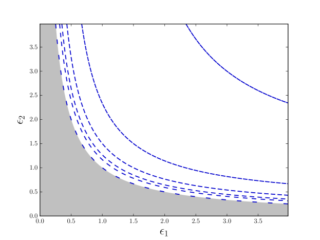
Figure 1: The space of parameters defined by $\epsilon_{1}\epsilon_{2}<1$ corresponds to the grey area. The dashed lines represent the extremal black holes where $r_{+}=r_{-}$, for $r_{+}=0.002,\,0.2,\,0.25,\,0.333,\,0.5,\,1$ with increasing dash density. The curve $r_{+}=1$, the one closest to the right upper corner, is drawn for comparison.

We will focus on the case $m_{1}=m_{2}=0$ (and therefore $\ell$ even) in order to keep the expressions reasonably short. It will be convenient to leave $z_{0}$ implicit at times,

$$z_{0}=\frac{r_{+}^{2}-r_{-}^{2}}{r_{+}^{2}-r_{0}^{2}}=\frac{1+(3+\epsilon_{1}+\epsilon_{2})r_{+}^{2}-\sqrt{(1+(1+\epsilon_{1}+\epsilon_{2})r_{+}^{2})^{2}+4\epsilon_{1}\epsilon_{2}r_{+}^{2}}}{1+(3+\epsilon_{1}+\epsilon_{2})r_{+}^{2}+\sqrt{(1+(1+\epsilon_{1}+\epsilon_{2})r_{+}^{2})^{2}+4\epsilon_{1}\epsilon_{2}r_{+}^{2}}},$$ (70)

which asymptotes as $z_{0}=(1-\epsilon_{1}\epsilon_{2})r_{+}^{2}+{\cal O}(r_{+}^{4})$. The expansions of the single monodromy parameters are, up to terms of order ${\cal O}(r_{+}^{3})$:

$$\theta_{0}=\omega\left(1-\frac{3}{2}(1+\epsilon_{1})(1+\epsilon_{2})r_{+}^{2}+\ldots\right)$$ (71)

$$\theta_{+}=i\omega\frac{(1+\epsilon_{1})(1+\epsilon_{2})}{1-\epsilon_{1}\epsilon_{2}}r_{+}+\ldots$$ (72)

$$\theta_{-}=-i\omega\frac{(1+\epsilon_{1})(1+\epsilon_{2})}{1-\epsilon_{1}\epsilon_{2}}\sqrt{\epsilon_{1}\epsilon_{2}}r_{+}+\ldots$$ (73)

The single monodromy parameters can be seen to have the structure:

$$\theta_{-}=-i\phi_{-}r_{+},\quad\quad\theta_{+}=i\phi_{+}r_{+},$$ (74)

where $\phi_{\pm}$ are real and positive for real and positive $\omega$. We also observe that $\theta_{0}$ is parametrically close to the frequency $\omega$, and the correction is negative for positive $r_{+}$.

We now proceed to solve for the composite monodromy parameter $\sigma_{\ell}\equiv\sigma_{0z_{0}}(\ell)$ using the series expansion (56). For even $\ell\geq 2$, the first correction is

$$\sigma_{\ell}\equiv \ell+2-\nu_{\ell}\,r_{+}^{2}$$

$$= \ell+2-\frac{(1+\epsilon_{1})(1+\epsilon_{2})}{4(\ell+1)}(3\omega^{2}+3\ell(\ell+2)-\Delta(\Delta-4))r_{+}^{2}+{\cal O}(r_{+}^{4}),\quad\ell\geq 2,$$ (75)

and, due to the pole structure of (57), naive series inversion will yield the expansion for $\sigma$ up to order $r_{+}^{2\ell}$. The case $\ell=0$ is then special, and will be dealt with shortly. One can see from (54) that, for $p=0$, the monodromy parameter $s$ will behave asymptotically as $z_{0}^{-\sigma}$, diverging for small $z_{0}$. Changing the value of $p$ will change this behavior. Changing the value of $p$ means shifting the argument $\sigma$ that enters the definition of $X_{0}(\sigma,t_{0})$ in (52) and therefore of $Y(\sigma,t_{0})$ in (48). Let us call $Y_{\ell,2p}$ the expression in (49) for generic $p$ and $\sigma\simeq 2+\ell$. The expression for $p=0$ is given by

$$Y_{\ell,0}\equiv Y(\sigma_{\ell};z_{0})=-(1-\epsilon_{1}\epsilon_{2})\frac{\omega^{2}-(\Delta-\ell-4)^{2}}{16(\ell+1)^{2}}\left(1+\frac{2i}{\ell+2}\phi_{+}r_{+}\right)r_{+}^{2}+\ldots,\quad\ell\geq 2.$$ (76)

We point out that this value is actually independent of $p$, except when $2p=\ell$, as we will see below. We anticipate, from (53), that $Y_{\ell,p}$ for $2p<\ell$ will yield a larger value for $s_{\ell}$ for smaller $r_{+}$. We also remark that $s_{\ell}$ will have a non-analytic expansion in $r_{+}$, due to the term $z_{0}^{-\sigma_{\ell}}$. Finally, from the expansion we conclude that $Y_{\ell,p}$ has an imaginary part of subleading order.

4.1 $\ell=0$

The “s-wave” case $\ell=0$ is singular since the leading behavior of $\sigma-2$ is of order $r_{+}^{2}$. The expansion (57) does not converge in general due to the denominator structure of the coefficients $\kappa_{n}$. For the small $r_{+}$ black hole application, however, we are really dealing with a scaling limit where

$$\theta_{-}=\varphi_{-}\sqrt{z_{0}},\quad\quad\theta_{+}=\varphi_{+}\sqrt{z_{0}},\quad\text{and}\quad\sigma=2-\upsilon z_{0}$$ (77)

have finite limits for $\varphi_{\pm}$ and $\upsilon$ as $z_{0}\rightarrow 0$. Because of the poles of increasing order in $\sigma$ in (57), in the $\ell=0$ case one has to resum the whole series in order to compute $\upsilon$.

Thankfully the task is amenable due to the fact that, in the scaling limit, the term of order $z_{0}$ in each of the factors $k_{n}t_{0}^{n}$ in the expansion (57) comes from the leading order pole (58)

$$k_{n}z_{0}^{n}=-4\mathbf{C}_{n-1}\frac{(\varphi_{-}^{2}-\varphi_{+}^{2})^{n}(\theta_{1}^{2}-\theta_{\infty}^{2})^{n}}{16^{n}\upsilon^{2n-1}}z_{0}+{\cal O}(z_{0}^{2}).$$ (78)

The series can be resummed using the generating function for the Catalan numbers

$$1+x+2x^{2}+5x^{3}+\ldots=\sum_{n=0}^{\infty}\mathbf{C}_{n}x^{n}=\frac{1-\sqrt{1-4x}}{2x}$$ (79)

and the result for $\upsilon$ readily written

$$4z_{0}K_{0}(\ell=0)+(\theta_{+}+\theta_{-}-1)^{2}+2(\theta_{1}-1)(\theta_{+}-1)\frac{z_{0}}{z_{0}-1}\\ =1+\frac{1}{2}(\theta_{1}^{2}-\theta_{\infty}^{2})z_{0}-2\upsilon z_{0}\sqrt{1+\frac{(\varphi_{+}^{2}-\varphi_{-}^{2})(\theta_{1}^{2}-\theta_{\infty}^{2})}{4\upsilon^{2}}}+{\cal O}(z_{0}^{2}).$$ (80)

A similar procedure allows us to compute the parameter $Y(\upsilon)\equiv Y(2-\upsilon z_{0};z_{0})$ up to order $z_{0}^{3/2}$:

$$Y(\upsilon)=-z_{0}(1+\varphi_{+}\sqrt{z_{0}})\frac{\theta_{\infty}^{2}-(\theta_{1}+2)^{2}}{64}\left(1+\sqrt{1+\frac{(\varphi_{+}^{2}-\varphi_{-}^{2})(\theta_{1}^{2}-\theta_{\infty}^{2})}{4\upsilon^{2}}}\right)^{2}+\ldots$$ (81)

For the application to the $\ell=0$ case of the scalar field, we will use the notation (74), and again use $\sigma_{0}=2-\nu_{0}r_{+}^{2}$. In terms of the black hole pameters, $\nu_{0}$ has a surprisingly simple form:

$$\nu_{0}=\frac{1}{4}(1+\epsilon_{1})(1+\epsilon_{2})\sqrt{(3\omega^{2}-\Delta(\Delta-4))^{2}-4\omega^{2}(\omega^{2}-(\Delta-2)^{2})}+{\cal O}(r_{+}^{2}),$$ (82)

and

$$Y_{0,0}\equiv Y(\sigma_{0};z_{0})=-(1-\epsilon_{1}\epsilon_{2})r_{+}^{2}\left(1+i\phi_{+}r_{+}\right)\frac{\omega^{2}-(\Delta-4)^{2}}{64}\\ \times\left(1+\frac{3\omega^{2}-\Delta(\Delta-4)}{\sqrt{(3\omega^{2}-\Delta(\Delta-4))^{2}-4\omega^{2}(\omega^{2}-(\Delta-2)^{2})}}\right)^{2}+\ldots$$ (83)

Finally, let us define the shifted $Y_{\ell,\ell}$ for $2p=\ell$. Since the shifted argument $\sigma-2p$ is close to $2$, we need the same scaling limit as above in (81). The result is

$$Y_{\ell,\ell}\equiv Y(\sigma_{\ell}-\ell;z_{0})=-(1-\epsilon_{1}\epsilon_{2})r_{+}^{2}\left(1+i\phi_{+}r_{+}\right)\frac{\omega^{2}-(\Delta-4)^{2}}{64}\\ \times\left(1+\sqrt{1+\frac{4(\ell+1)^{2}\omega^{2}(\omega^{2}-(\Delta-2)^{2})}{(3\omega^{2}+3\ell(\ell+2)-\Delta(\Delta-4))^{2}}}\right)^{2}+\ldots,$$ (84)

where $\nu_{\ell}$ is taken from (75).

To sum up, we exhibit the overall structure for small $r_{+}$:

$$\sigma_{\ell}=\ell+2-\nu_{\ell}r_{+}^{2}+\ldots,$$ (85)

$$Y_{\ell,\ell}=-(1-\epsilon_{1}\epsilon_{2})\vartheta_{\ell}\left(1+i\phi_{+}r_{+}\right)r_{+}^{2}+\ldots,$$ (86)

where $\nu_{\ell}$ and $\vartheta_{\ell}$ have non-zero limits as $r_{+}\rightarrow 0$, corrections of order $r_{+}^{2}$, and, most importantly, are positive for $\omega$ real and greater than $\Delta-4$.

4.2 The quasinormal modes

Implementation of the quantization condition (40) can be done with the formula (129). This yields a transcendental equation for $\omega$ whose solutions will give all complex frequencies for the radial quantization condition. These include negative-real part frequencies, as well as non-normalizable modes. Since we are interested in positive real-part frequencies, we will consider a small correction to the vacuum $\mathrm{AdS}_{5}$ result Aharony:1999ti ; Penedones:2016voo

$$\omega_{n,\ell}=\Delta+2n+\ell+\eta_{n,\ell}\,r_{+}^{2},$$ (87)

under the hypothesis that $\eta_{n,\ell}$ has a finite limit as $r_{+}\rightarrow 0$. One notes by (71) that $\theta_{0}$ and $\omega$ are perturbatively close, so $\eta_{n,\ell}$ can be calculated perturbatively from the expansion of $\theta_{0}$. We will assume that $\Delta$ is not an integer.

The parametrization (87) allows us to expand (54) as a function of $r_{+}$. The procedure is straightforward: We use $Y_{\ell,0}$ from (86), as it gives the right asymptotic behavior, to compute $X_{0}$ using (48) and then the $s$ parameter (54). To second order in $r_{+}$ we have

$$s_{n,\ell}=-\frac{16\,\Gamma(n+\ell/2+1)\Gamma(\Delta-2+n+\ell/2)}{\Gamma(n+\ell/2+3)\Gamma(\Delta+n+\ell/2)}\frac{\nu_{\ell}^{2}}{(1-\epsilon_{1}\epsilon_{2})^{2}(\phi_{+}^{2}-\phi_{-}^{2})}\\ \times\left(1-i\phi_{+}r_{+}+2i\frac{\phi_{+}\nu_{\ell}r_{+}}{\phi_{+}^{2}-\phi_{-}^{2}}\right)Y_{\ell,\ell}r_{+}^{-2+2\nu_{\ell}r_{+}^{2}},$$ (88)

and the leading behavior for the parameter $s_{n,\ell}$ given $Y_{\ell,\ell}$ in (86) is

$$s_{n,\ell}=\Sigma_{n,\ell}\left(1+\frac{2i\nu_{n,\ell}r_{+}}{(1+\epsilon_{1})(1+\epsilon_{2})(\Delta+2n+\ell)}\right)r_{+}^{2\nu_{n,\ell}r_{+}^{2}}+\ldots,$$ (89)

where we defined $\nu_{n,\ell}$ as the correction for $\sigma$ as in (86) calculated at the vacuum frequency $\nu_{\ell}(\omega=\Delta+2n+\ell)$. Finally,

$$\Sigma_{n,\ell}=\frac{16\,\Gamma(n+\ell/2+1)\Gamma(\Delta-2+n+\ell/2)}{\Gamma(n+\ell/2+3)\Gamma(\Delta+n+\ell/2)}\frac{\nu_{n,\ell}^{2}\,\vartheta_{n,\ell}}{(1+\epsilon_{1})^{2}(1+\epsilon_{2})^{2}(\Delta+2n+\ell)^{2}},$$ (90)

again, with $\vartheta_{n,\ell}=\vartheta(\omega=\Delta+2n+\ell)$. We also note that $\Sigma_{n,\ell}$ is real and positive under the same conditions as (86). Moreover, the choice of $p$, implicit in $Y_{\ell,\ell}$ guarantees that $s_{n,\ell}$ has a finite limit as $r_{+}\rightarrow 0$, although its dependence on $r_{+}$ is non-analytic.

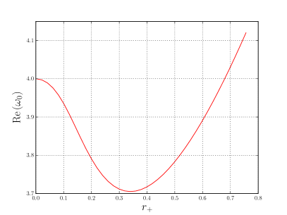
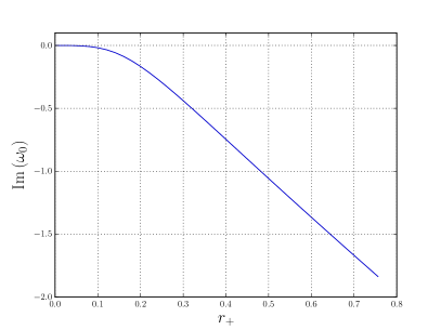
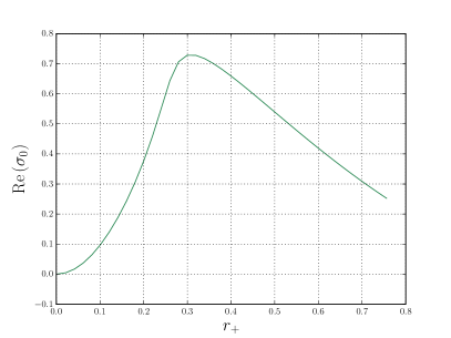
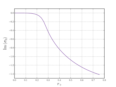
Figure 2: In the first row, the dependence of the real and imaginary parts of the first quasinormal mode frequency $\omega_{0}$ for small Kerr-AdS₅ black holes ($a_{1}=0.002,a_{2}=0.00199,\mu=7.96\times 10^{-8}$ ). In the second, the dependence of the composite parameter $2-\sigma$.

Equation (129) can now be used, setting $\cos\pi\sigma_{1t}=\cos\pi(\theta_{1}+\theta_{t})$ for the radial parameters, to find a perturbative equation for $\eta_{n,\ell}$. We expand each of the terms in (129) using (74) as well as

$$\theta_{0}=\omega_{0}-\beta r_{+}^{2},\quad\omega_{0}=\Delta+2n+\ell,\quad\text{and}\quad\sigma=2+\ell-\nu_{\ell}r_{+}^{2}.$$ (91)

Now, the following two relations hold

$$\sin^{2}\pi\sigma\cos\pi(\theta_{1}+\theta_{t})-\cos\pi\theta_{0}\cos\pi\theta_{\infty}-\cos\pi\theta_{t}\cos\pi\theta_{1}\\ +\cos\pi\sigma(\cos\pi\theta_{0}\cos\pi\theta_{1}+\cos\pi\theta_{t}\cos\pi\theta_{\infty})=\\ \frac{\pi^{3}}{2}\sin(\pi\Delta)(\phi_{+}^{2}-\phi_{-}^{2})\left(\beta+\frac{2i\nu_{\ell}^{2}r_{+}}{(1+\epsilon_{1})(1+\epsilon_{2})\omega_{0}}\right)r_{+}^{4}+\ldots$$ (92)

$$-\frac{1}{2}(\cos\pi\theta_{\infty}-\cos\pi(\theta_{1}\pm\sigma))(\cos\pi\theta_{0}-\cos\pi(\theta_{t}\pm\sigma))=\\ \frac{\pi^{3}}{2}\sin(\pi\Delta)(\phi_{+}^{2}-\phi_{-}^{2})\left(\frac{\beta\pm\nu}{2}\right)\left(1\pm\frac{2i\nu_{\ell}r_{+}}{(1+\epsilon_{1})(1+\epsilon_{2})\omega_{0}}\right)r_{+}^{4}+\ldots$$ (93)

We can now proceed to calculate the first correction to the eigenfrequencies (87). By using the approximations (92) and (93) above we find the correction to $\theta_{0}$ for each of the modes $n,\ell$

$$\beta_{n,\ell}=\nu_{n,\ell}\frac{\Sigma_{n,\ell}+1}{\Sigma_{n,\ell}-1}+4i\frac{\nu_{n,\ell}^{2}}{(1+\epsilon_{1})(1+\epsilon_{2})(\Delta+2n+\ell)}\frac{\Sigma_{n,\ell}}{(\Sigma_{n,\ell}-1)^{2}}r_{+}+{\cal O}(r_{+}^{2}\log r_{+}).$$ (94)

Finally, after some laborious calculations, we find

$$\eta_{n,\ell}=-\frac{(1+\epsilon_{1})(1+\epsilon_{2})}{2}\left[\frac{Z_{n,\ell}}{2(\ell+1)}-3(\Delta+2n+\ell)\right]\\ -\frac{i}{4}(2n+\ell+1)(1+\epsilon_{1})(1+\epsilon_{2})(\Delta+2n+\ell)(2\Delta+2n+\ell-2)r_{+}\\ +{\cal O}(r_{+}^{2}\log r_{+}),\quad\quad\ell\geq 2,$$ (95)

with

$$Z_{n,\ell}^{2}=(3(\Delta+2n+\ell)^{2}+3\ell(\ell+2)-\Delta(\Delta-4))^{2}\\ +4(\ell+1)^{2}(\Delta+2n+\ell)^{2}(2n+\ell+1)(2\Delta+2n+\ell-2).$$ (96)

For $\ell=0$, the form of the correction is slightly different. Repeating the calculation, we see that $\eta_{n,\ell=0}$ has the simpler form

$$\eta_{n,0}=-\frac{(1+\epsilon_{1})(1+\epsilon_{2})}{4}(3(\Delta+2n-1)^{2}-(\Delta-2)^{2}+1)\\ -i(n+1)(1+\epsilon_{1})(1+\epsilon_{2})(\Delta+2n)(\Delta+n-1)r_{+}+{\cal O}(r_{+}^{2}\log r_{+}).$$ (97)

We note that both the real and imaginary parts of the corrections $\eta_{n,\ell}$ are negative, the real part of order $r_{+}^{2}$ as expected, and the imaginary part of order $r_{+}^{3}$. We stress that we are taking $m_{1}=m_{2}=0$.

In the midst of the calculation, we see that the imaginary part of $\eta_{n,0}$ has the same sign as the imaginary part of $\theta_{+}$, which in turn is essentially the entropy intake of the black hole as it absorbs a quantum of frequency $\omega$ and angular momenta $m_{1}$ and $m_{2}$:

$$\theta_{+}=\frac{i}{2\pi}\delta S=\frac{i}{2\pi}\frac{\omega-m_{1}\Omega_{+,1}-m_{2}\Omega_{+,2}}{T_{+}}$$ (98)

giving the same sort of window for unstable modes parameters $m_{1},m_{2}$ as in superradiance, so a closer look at higher values for $m_{1,2}$ is perhaps in order for future work. A full consideration of linear perturbations of the five-dimensional Kerr-AdS black hole, involving higher spin Wu:2009ug ; Lunin:2017drx , can be done within the same theoretical framework presented here, and will be left for the future. We close by observing that the expressions (95) and (97) above seem to represent a distinct limit than the results in Aliev:2008yk – which are, however, restricted to $\Delta=4$ – and therefore not allowing for a direct comparison.

4.3 Some words about the $\ell$ odd case

Let us illustrate the parameters for the subcase $m_{1}=\ell,m_{2}=0$. The single monodromy parameters admit the expansion

$$\theta_{0}=\omega+\sqrt{\epsilon_{1}}\ell r_{+}-\frac{3}{2}(1+\epsilon_{1})(1+\epsilon_{2})\omega r_{+}^{2}+\ldots$$ (99)

$$\theta_{+}=-i\ell\frac{\sqrt{\epsilon_{1}}(1+\epsilon_{2})}{1-\epsilon_{1}\epsilon_{2}}+i\omega\frac{(1+\epsilon_{1})(1+\epsilon_{2})}{1-\epsilon_{1}\epsilon_{2}}r_{+}+\ldots$$ (100)

$$\theta_{-}=i\ell\frac{\sqrt{\epsilon_{2}}(1+\epsilon_{1})}{1-\epsilon_{1}\epsilon_{2}}-i\omega\frac{(1+\epsilon_{1})(1+\epsilon_{2})}{1-\epsilon_{1}\epsilon_{2}}\sqrt{\epsilon_{1}\epsilon_{2}}r_{+}+\ldots,$$ (101)

with all of them finite and non-zero as $r_{+}\rightarrow 0$. As usual, $\theta_{\pm}$ are purely imaginary whereas $\theta_{0}$ is real for real $\omega$. These properties hold for any value of $m_{1}$ and $m_{2}$.

For $\ell\geq 1$ and odd, the composite monodromy parameters are found much in the same way as the case $\ell\geq 2$ considered above, by inverting (56). In the following we set $\omega_{0}=\Delta+2n+\ell$ as the limit of the frequency as $r_{+}\rightarrow 0$. We have for the composite monodromy parameter

$$\sigma_{\ell}=2+\ell-\nu_{\ell}r_{+}^{2}+{\cal O}(r_{+}^{4}),$$ (102)

with $\nu_{\ell}$, defined as in (89), now for $\ell>1$

$$\nu_{\ell}=(1+\epsilon_{1})(1+\epsilon_{2})\frac{3\omega_{0}^{2}+3\ell(\ell+2)-\Delta(\Delta-4)}{4(\ell+1)},\quad\quad\ell\geq 3.$$ (103)

For $\ell=1$, finding $\nu_{1}$ from condition (41) requires going to higher order in $z_{0}$, due to the pole at $\sigma=3$ in the expansion (56),

$$\nu_{1}=\frac{(1+\epsilon_{1})(1+\epsilon_{2})}{32}(3\omega_{0}^{2}+9-\Delta(\Delta-4))\\ \times\left(2+\frac{1}{3}\sqrt{34-8\frac{2\Delta^{4}-16\Delta^{3}+(50-3\omega_{0}^{2})\Delta^{2}+12(\omega_{0}^{2}-6)\Delta-36\omega_{0}^{2}}{(3\omega_{0}^{2}+9-\Delta(\Delta-4))^{2}}}\right).$$ (104)

For the following discussion, we take from this calculation that the $\nu_{\ell}$’s are real and greater than $1$ for $\Delta>1$, which we will assume to hold for any $m_{1}$ and $m_{2}$. Apart from these properties, the particular form for $\nu_{\ell}$ will be left implicit. Given $\nu_{\ell}$, we can use the same procedure as in the even $\ell$ case to compute the $s$ parameter. Again, in order to have a finite $r_{+}\rightarrow 0$ limit, we take $p=(\ell+1)/2$. After some calculations, we have

$$s_{n,\ell}=1+2\nu_{\ell}r_{+}^{2}\log r_{+}+\Xi_{n,\ell}\nu_{\ell}r_{+}^{2}+{\cal O}(r_{+}^{4}(\log r_{+})^{2})$$ (105)

with

$$\Xi_{n,\ell}=2\gamma+\log(1-\epsilon_{1}\epsilon_{2})+\Psi\left(\frac{1+\theta_{+}+\theta_{-}}{2}\right)+\Psi\left(\frac{1+\theta_{+}-\theta_{-}}{2}\right)\\ +\Psi\left(\frac{3+2n+\ell}{2}\right)+\Psi\left(\frac{3-2\Delta-2n-\ell}{2}\right),$$ (106)

where $\Psi(z)$ is the digamma function, and $\gamma=-\Psi(1)$ the Euler-Mascheroni constant. In the definition above we have already set $\theta_{0}=\Delta+2n+\ell-\beta_{n,\ell}r_{+}^{2}$, but as we can see from (105), now we need $s_{n,\ell}$ to second order in the expansion parameter $r_{+}$. We again assume that $\Delta$ is in general not an integer, since this is irrelevant for the determination of the imaginary part of the frequency. However, having $\Delta$ integer will change the behavior of the real part of the correction to the eigenfrequency with respect to $r_{+}$.

We note that $s_{n,\ell}$ is non-analytic, and therefore the expansion for $\beta_{n,\ell}$ will include terms like $\log r_{+}$. We expand (129), with $\sigma_{1t}=2-\Delta+\theta_{+}$ (up to an even integer) to fourth order and find as first approximation to the correction to the frequency

$$\eta_{n,\ell}=\ldots+\nu_{n,\ell}\left(\frac{\nu_{n,\ell}+1}{\nu_{n,\ell}-1}+\Xi_{n,\ell}\right)\frac{r_{+}^{2}}{\log r_{+}}+\ldots,$$ (107)

where the terms left out are real, stemming from the relation between $\theta_{0}$ and $\omega$.

From (107), any possible imaginary part for the eigenfrequency will then come from the imaginary part of $\Xi_{n,\ell}$. The latter can be calculated by using the reflexion property of the digamma function

$$\Im\Xi_{n,\ell}=-\frac{i\pi}{2}\left(\tan\frac{\pi}{2}(\theta_{+}+\theta_{-})+\tan\frac{\pi}{2}(\theta_{+}-\theta_{-})\right),$$ (108)

or, in terms of $m_{1}$ and $m_{2}$,

$$\Im\Xi_{n,\ell}=\frac{\pi}{2}\tanh\left(\frac{\pi}{2}\frac{\sqrt{\epsilon_{1}}-\sqrt{\epsilon_{2}}}{1+\sqrt{\epsilon_{1}\epsilon_{2}}}(m_{1}-m_{2})\right)+\frac{\pi}{2}\tanh\left(\frac{\pi}{2}\frac{\sqrt{\epsilon_{1}}+\sqrt{\epsilon_{2}}}{1-\sqrt{\epsilon_{1}\epsilon_{2}}}(m_{1}+m_{2})\right).$$ (109)

We then see that the imaginary part of $\Xi_{n,\ell}$ can have any sign, a strong indication that the $\ell$ odd modes are unstable. Numerical support for this is included in Fig. 3, in which we use an arbitrary-precision Python code (capped at 50 decimal places) to show a slightly positive imaginary part for the resonant frequency at $r\lesssim 0.02$. We point out that, indeed, instabilities in asymptotically anti-de Sitter spaces are expected from general grounds Green:2015kur , and odd $\ell$ instabilities for the massless case ($\Delta=4$) were found in Aliev:2008yk .

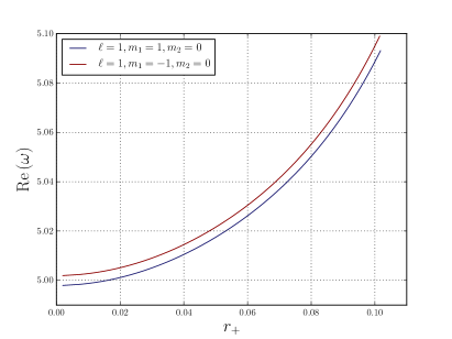
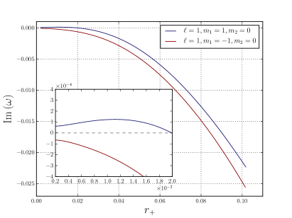
Figure 3: The dependence of the real (left) and imaginary part (right) of the first quasinormal mode frequency $\omega_{0}$ at $\ell=1$ and $m_{1}=\pm 1$ for small Kerr-AdS₅ black holes ($a_{1}=0.002,a_{2}=0.00199,\mu=7.96\times 10^{-8}$ ).

5 Discussion

In this paper we used the isomonodromy method to derive asymptotic expressions for the separation constant for the angular equation (angular eigenvalue) in (63) as well as the frequencies for the scalar quasinormal modes in a five-dimensional Kerr-AdS background in the limit of small black holes, see in particular (95) and (97). The numerical analysis carried out for the Schwarzschild-AdS and Kerr-AdS cases showed that the $\tau$ function approach has advantages when compared to standard methods, in terms of faster processing times. For $\ell$ even, the correction to the vacuum AdS frequencies is negative with negative imaginary part for $\Delta>1$, the scalar unitarity bound, showing no instability in the range studied. For $\ell$ odd, there are strong indications for instability due to the general structure of the corrections in (109). In particular, for $\ell=1$, the numerical results shown in Fig. 3 exhibit an unstable mode for $r_{+}\leq 0.02$ and nearly equal rotational parameters. We plan to address the phase space of instabilities and holographic consequences in future work.

The method in this paper relies on the construction of the $\tau$ function of the PVI transcendent proposed in the literature following the AGT conjecture. The conditions in (41) translate the accessory parameters in the ODEs governing the propagation of the field – themselves depending on the physical parameters – into monodromy parameters, and the quantization condition (39) allows us to derive the angular separation constant (63). In turn, the quantization condition for the radial equation (40), through series solutions for the composite monodromy parameters $s$ and $\sigma$, allows us to solve for the eigenfrequencies $\omega_{n,\ell}$, even in the generic complex case.

The interpretation of the ODEs involved as the level 2 null vector condition of semi-classical Liouville field theory allows us to conclude that all descendants are relevant for the calculation of the monodromy parameters, even though for angular momentum parameter $\ell\geq 2$, one can consider just the conformal primary (first channel) for the parameter $\sigma_{0t}$.

The scaling limit resulting from this analysis gives the monodromy parameter $\sigma$ in (75). For the parameter $\sigma_{1t}$, the requisite of a smooth $r_{+}\rightarrow 0$ limit forces us to consider the asymptotics of the whole series (56), thus involving all descendants. This means that naive matching of the solution obtained from the near horizon approximation to the asymptotic solution near infinity is not a suitable tool for dealing with small black holes. For the composite monodromy parameter $\sigma_{1t}$, more suitably parametrized by $s$ in (129), the requirement of a finite $r_{+}\rightarrow 0$ limit allows us to select the solutions (89) for $\ell$ even and (105) for $\ell$ odd. Although finite in the small black hole limit, the $s$ parameter has a non-analytic expansion in terms of $r_{+}^{m}(\log r_{+})^{n}$.

For the s-wave $\ell=0$ calculations, we had to consider a scaling limit in (56) where the Liouville momenta associated to $\theta_{+}$ and $\theta_{-}$ go to zero as $r_{+}$, at the same time as $z_{0}$ and $\sigma-2$ scales as $r_{+}^{2}$. The formulas (80) and (81) are reminiscent of the light-light-heavy-heavy limit of Witten diagrams for conformal blocks Hijano:2015zsa . It would be interesting to understand the CFT meaning of this limit.

The Toda equation, which allows us to interpret the second condition (41) on the Painlevé $\tau$ function, also merits further study. As for the first condition, we note that it provides the accessory parameters for both the angular and radial equations – $Q_{0}$ in (12) and $K_{0}$ in (20), respectively – as the derivative of the logarithm of the $\tau$ function for each system. On the other hand, these accessory parameters are both related to the separation constant of the Klein-Gordon equation, as can be verified through (14) and (22). Including these terms in the definition of a $\tau$ function for the angular and radial systems, we can represent the fact that the separation constant is the same for (12) and (20) as the condition

$$\frac{d}{du_{0}}\log\tau_{\mathrm{angular}}=\frac{d}{dz_{0}}\log\tau_{\mathrm{radial}},$$ (110)

which in turn can be interpreted as a thermodynamical equilibrium condition. Given the usual interpretation of the $\tau$ function as the generating functional of a quantum theory, the elucidation of this structure can shed light on the spacetime approach to conformal blocks. The present work gives, in our opinion, convincing evidence that the PVI $\tau$ function is the best tool – both numerically and analytically – to study connection problems for Fuchsian equations, in particular scattering and resonance problems for a wide class of black holes.

Appendix A Nekrasov expansion and Fredholm determinant for Painlevé VI

In what follows, we will assume the “sufficient generality condition”

$$\sigma_{0t}\notin\mathbb{Z},\quad\sigma_{0t}\pm\theta_{0}\pm\theta_{t}\notin\mathbb{Z},\quad\sigma_{0t}\pm\theta_{1}\pm\theta_{\infty}\notin\mathbb{Z}.$$ (111)

The Nekrasov expansion of the PVI $\tau$ function is given as a double expansion Gamayun:2013auu ; Anselmo20180080

$$\tau(t)=\sum_{n\in\mathbb{Z}}{\cal N}^{\theta_{1}}_{\theta_{\infty},\sigma_{0t}+2n}{\cal N}^{\theta_{t}}_{\sigma_{0t}+2n,\theta_{0}}s^{n}t^{\tfrac{1}{4}((\sigma_{0t}+2n)^{2}-\theta_{0}^{2}-\theta_{t}^{2})}(1-t)^{\tfrac{1}{2}\theta_{1}\theta_{t}}\sum_{\lambda,\mu\in\mathbb{Y}}{\cal B}_{\lambda,\mu}(\vec{\theta},\sigma_{0t}+2n)t^{|\lambda|+|\mu|},$$ (112)

where

$${\cal N}^{\theta_{3}}_{\theta_{2},\theta_{1}}=\frac{\prod_{\epsilon=\pm}G(1+\tfrac{1}{2}(\theta_{3}+\epsilon(\theta_{2}+\theta_{1})))G(1+\tfrac{1}{2}(\theta_{3}+\epsilon(\theta_{2}-\theta_{1})))}{G(1-\theta_{1})G(1+\theta_{2})G(1-\theta_{3})}$$ (113)

with $G(z)$ the Barnes function, defined by the solution of the functional equation $G(z+1)=\Gamma(z)G(z)$, with $G(1)=1$ and $\Gamma(z)$ the Euler gamma. The other parameters in (112) are the coefficients of the $c=1$ Virasoro conformal block

$${\cal B}_{\lambda,\mu}(\vec{\theta},\sigma)=\prod_{(i,j)\in\lambda}\frac{((\theta_{t}+\sigma+2(i-j))^{2}-\theta_{0}^{2})((\theta_{1}+\sigma+2(i-j))^{2}-\theta_{\infty}^{2})}{16h_{\lambda}^{2}(i,j)(\lambda^{\prime}_{j}-i+\mu_{i}-j+1+\sigma)^{2}}\times\\ \prod_{(i,j)\in\mu}\frac{((\theta_{t}-\sigma+2(i-j))^{2}-\theta_{0}^{2})((\theta_{1}-\sigma+2(i-j))^{2}-\theta_{\infty}^{2})}{16h_{\lambda}^{2}(i,j)(\mu^{\prime}_{j}-i+\lambda_{i}-j+1-\sigma)^{2}},$$ (114)

where $\mathbb{Y}$ denote the space of Young diagrams, $\lambda$ and $\mu$ are two of its elements, with number of boxes $|\lambda|$ and $|\mu|$. For each box situated at $(i,j)$ in $\lambda$, $\lambda_{i}$ are the number of boxes at row $i$ of $\lambda$, $\lambda^{\prime}_{j}$, the number of boxes at column $j$ of $\lambda$; $h(i,j)=\lambda_{i}+\lambda^{\prime}_{j}-i-j+1$ is the hook length of the box at $(i,j)$. Finally, the parameter $s$ is given in terms of monodromy data by:

$$s=\frac{(w_{1t}-2p_{1t}-p_{0t}p_{01})-(w_{01}-2p_{01}-p_{0t}p_{1t})\exp({\pi i\sigma_{0t}})}{(2\cos\pi(\theta_{t}-\sigma_{0t})-p_{0})(2\cos\pi(\theta_{1}-\sigma_{0t})-p_{\infty})}$$ (115)

where

$$\begin{gathered}p_{i}=2\cos\pi\theta_{i},\quad p_{ij}=2\cos\pi\sigma_{ij},\\ w_{0t}=p_{0}p_{t}+p_{1}p_{\infty},\quad w_{1t}=p_{1}p_{t}+p_{0}p_{\infty},\quad w_{01}=p_{0}p_{1}+p_{t}p_{\infty}.\end{gathered}$$ (116)

The Fredholm determinant representation for the PVI $\tau$ function uses the usual Riemann-Hilbert problem formulation in terms of Plemelj (projection) operators and jump matrices. The idea is to introduce projection operators which act on the space of (pair of) functions on the complex plane to give analytic functions with prescribed monodromy (Cauchy-Riemann operators). Details can be found in Gavrylenko:2016zlf . One should point out that the two expansions agree as functions of $t$ up to a multiplicative constant.

$$\tau(t)=\mathrm{const.}\cdot t^{\frac{1}{4}(\sigma^{2}-\theta_{0}^{2}-\theta_{t}^{2})}(1-t)^{-\frac{1}{2}\theta_{t}\theta_{1}}\det(\mathbbold{1}-AD),$$ (117)

where the Plemelj operators $A,D$ act on the space of pairs of square-integrable functions defined on ${\cal C}$, a circle on the complex plane with radius $R<1$:

$$(Ag)(z)=\oint_{\cal C}\frac{dz^{\prime}}{2\pi i}A(z,z^{\prime})g(z^{\prime}),\quad(Dg)(z)=\oint_{\cal C}\frac{dz^{\prime}}{2\pi i}D(z,z^{\prime})g(z^{\prime}),\quad g(z^{\prime})=\begin{pmatrix}f_{+}(z)\\ f_{-}(z)\end{pmatrix}$$ (118)

with kernels given, for $|t|<R$, explicitly by

$$\begin{gathered}A(z,z^{\prime})=\frac{\Psi(\theta_{1},\theta_{\infty},\sigma;z)\Psi^{-1}(\theta_{1},\theta_{\infty},\sigma;z^{\prime})-\mathbbold{1}}{z-z^{\prime}},\\ D(z,z^{\prime})=\Phi(t)\frac{\mathbbold{1}-\Psi(\theta_{t},\theta_{0},-\sigma;t/z)\Psi^{-1}(\theta_{t},\theta_{0},-\sigma;t/z^{\prime})}{z-z^{\prime}}\Phi^{-1}(t).\end{gathered}$$ (119)

The parametrix $\Psi(z)$ and the “gluing” matrix $\Phi(t)$ are

$$\leavevmode\resizebox{422.77661pt}{}{$\displaystyle\Psi(\alpha_{1},\alpha_{2},\alpha_{3};z)=\begin{pmatrix}\phi(\alpha_{1},\alpha_{2},\alpha_{3};z)&\chi(\alpha_{1},\alpha_{2},\alpha_{3};z)\\ \chi(\alpha_{1},\alpha_{2},-\alpha_{3};z)&\phi(\alpha_{1},\alpha_{2},-\alpha_{3},z)\end{pmatrix},\quad\Phi(t)=\begin{pmatrix}t^{-\sigma/2}\kappa^{-1/2}&0\\ 0&t^{\sigma/2}\kappa^{1/2}\end{pmatrix}$},$$ (120)

with $\phi$ and $\chi$ given in terms of Gauss’ hypergeometric function:

Finally, $\kappa$ is a known function of the monodromy parameters:

$$\kappa=s\frac{\Gamma^{2}(1-\sigma)}{\Gamma^{2}(1+\sigma)}\frac{\Gamma(1+\tfrac{1}{2}(\theta_{t}+\theta_{0}+\sigma))\Gamma(1+\tfrac{1}{2}(\theta_{t}-\theta_{0}+\sigma))}{\Gamma(1+\tfrac{1}{2}(\theta_{t}+\theta_{0}-\sigma))\Gamma(1+\tfrac{1}{2}(\theta_{t}-\theta_{0}-\sigma))}\times\\ \frac{\Gamma(1+\tfrac{1}{2}(\theta_{1}+\theta_{\infty}+\sigma))\Gamma(1+\tfrac{1}{2}(\theta_{1}-\theta_{\infty}+\sigma))}{\Gamma(1+\tfrac{1}{2}(\theta_{1}+\theta_{\infty}-\sigma))\Gamma(1+\tfrac{1}{2}(\theta_{1}-\theta_{\infty}-\sigma))}.$$ (122)

Meaningful limits for integer $\sigma$, violating (111) can be obtained by cancelling the factors in the denominator of $s$ with poles of the Barnes function from the structure constants ${\cal N}^{\sigma+2n}_{\theta_{t},\theta_{0}}$.

For the numerical implementation, we write the matrix elements of $A$ and $D$ in the Fourier basis $z^{n}$, truncated up to order $N$. Again, the structure of the matrix elements $A_{mn}$ and $D_{mn}$ can be found in Gavrylenko:2016zlf . This truncation gives $\tau$ up to terms ${\cal O}(t^{N})$, and, unlike the Nekrasov expansion, can be computed in polynomial time. The formulation does in principle allow for calculation for arbitrary values of $t$, by evaluating the integrals in (118) as Riemann sums using quadratures Bornemann:2009aa , so there are good perspectives for using the method outlined here for more generic configurations.

Appendix B Explicit monodromy calculations

Given $\sigma_{0t}$ and $s$, satisfying (111) we can construct an explicit representation for the monodromy matrices – up to conjugation – as follows.

The monodromy matrices are

The matrices satisfy

$$M_{t}M_{0}=\begin{pmatrix}e^{i\pi\sigma_{0t}}&0\\ 0&e^{-i\pi\sigma_{0t}}\end{pmatrix},\quad\quad M_{\infty}M_{1}=\begin{pmatrix}e^{-i\pi\sigma_{0t}}&0\\ 0&e^{i\pi\sigma_{0t}}\end{pmatrix}.$$ (127)

The parameters $s_{i},s_{e}$ are related to the parameter $s$ defined in (115) through:

$$s=\frac{s_{i}}{s_{e}}.$$ (128)

A direct calculation shows that

$$\sin^{2}\pi\sigma_{0t}\cos\pi\sigma_{1t}=\cos\pi\theta_{0}\cos\pi\theta_{\infty}+\cos\pi\theta_{t}\cos\pi\theta_{1}\\ -\cos\pi\sigma_{0t}(\cos\pi\theta_{0}\cos\pi\theta_{1}+\cos\pi\theta_{t}\cos\pi\theta_{\infty})\\ -\frac{1}{2}(\cos\pi\theta_{\infty}-\cos\pi(\theta_{1}-\sigma_{0t}))(\cos\pi\theta_{0}-\cos\pi(\theta_{t}-\sigma_{0t}))s\\ -\frac{1}{2}(\cos\pi\theta_{\infty}-\cos\pi(\theta_{1}+\sigma_{0t}))(\cos\pi\theta_{0}-\cos\pi(\theta_{t}+\sigma_{0t}))s^{-1}$$ (129)

We close by noting that for the special case of interest where $\sigma_{1t}=\theta_{1}+\theta_{t}+2n$, $n\in\mathbb{Z}$, the expressions above are still valid.

References

- (1) J. B. Amado, B. Carneiro da Cunha, and E. Pallante, On the Kerr-AdS/CFT correspondence, JHEP 08 (2017) 094, [arXiv:1702.01016].
- (2) A. Nunez and A. O. Starinets, AdS / CFT correspondence, quasinormal modes, and thermal correlators in N=4 SYM, Phys. Rev. D67 (2003) 124013, [hep-th/0302026].
- (3) E. Berti, V. Cardoso, and A. O. Starinets, Quasinormal modes of black holes and black branes, Class. Quant. Grav. 26 (2009) 163001, [arXiv:0905.2975].
- (4) S. W. Hawking, C. J. Hunter, and M. Taylor, Rotation and the AdS / CFT correspondence, Phys. Rev. D59 (1999) 064005, [hep-th/9811056].
- (5) S. W. Hawking and H. S. Reall, Charged and rotating AdS black holes and their CFT duals, Phys. Rev. D61 (2000) 024014, [hep-th/9908109].
- (6) K. Landsteiner and E. Lopez, The Thermodynamic potentials of Kerr-AdS black holes and their CFT duals, JHEP 12 (1999) 020, [hep-th/9911124].
- (7) V. Cardoso and O. J. C. Dias, Small Kerr-anti-de Sitter black holes are unstable, Phys. Rev. D70 (2004) 084011, [hep-th/0405006].
- (8) A. N. Aliev and O. Delice, Superradiant Instability of Five-Dimensional Rotating Charged AdS Black Holes, Phys. Rev. D79 (2009) 024013, [arXiv:0808.0280].
- (9) N. Uchikata, S. Yoshida, and T. Futamase, Scalar perturbations of Kerr-AdS black holes, Phys. Rev. D80 (2009) 084020.
- (10) F. Novaes and B. Carneiro da Cunha, Isomonodromy, Painlevé transcendents and scattering off of black holes, JHEP 07 (2014) 132, [arXiv:1404.5188].
- (11) B. Carneiro da Cunha and F. Novaes, Kerrde Sitter greybody factors via isomonodromy, Phys. Rev. D93 (2016), no. 2 024045, [arXiv:1508.04046].
- (12) F. Novaes, C. Marinho, M. Lencsés, and M. Casals, Kerr-de Sitter Quasinormal Modes via Accessory Parameter Expansion, arXiv:1811.11912.
- (13) O. Gamayun, N. Iorgov, and O. Lisovyy, Conformal field theory of Painlevé VI, JHEP 10 (2012) 038, [arXiv:1207.0787]. [Erratum: JHEP10,183(2012)].
- (14) M. Jimbo, Monodromy Problem and the boundary condition for some Painlevé equations, Publ. Res. Inst. Math. Sci. 18 (1982) 1137–1161.
- (15) P. Gavrylenko and O. Lisovyy, Fredholm Determinant and Nekrasov Sum Representations of Isomonodromic Tau Functions, Commun. Math. Phys. 363 (2018) 1–58, [arXiv:1608.00958].
- (16) M. Cafasso, P. Gavrylenko, and O. Lisovyy, Tau functions as Widom constants, arXiv:1712.08546.
- (17) G. W. Gibbons, M. J. Perry, and C. N. Pope, The First law of thermodynamics for Kerr-anti-de Sitter black holes, Class. Quant. Grav. 22 (2005) 1503–1526, [hep-th/0408217].
- (18) S. Hollands, A. Ishibashi, and D. Marolf, Comparison between various notions of conserved charges in asymptotically AdS-spacetimes, Class. Quant. Grav. 22 (2005) 2881–2920, [hep-th/0503045].
- (19) R. Olea, Regularization of odd-dimensional AdS gravity: Kounterterms, JHEP 04 (2007) 073, [hep-th/0610230].
- (20) M. Jimbo and T. Miwa, Monodromy Preserving Deformation of Linear Ordinary Differential Equations with Rational Coefficients, II, Physica D2 (1981) 407–448.
- (21) K. Iwasaki, H. Kimura, S. Shimomura, and M. Yoshida, From Gauss to Painlevé: A Modern Theory of Special Functions, vol. 16 of Aspects of Mathematics E. Braunschweig, 1991.
- (22) O. Gamayun, N. Iorgov, and O. Lisovyy, How instanton combinatorics solves Painlevé VI, V and IIIs, J. Phys. A46 (2013) 335203, [arXiv:1302.1832].
- (23) T. Anselmo, R. Nelson, B. Carneiro da Cunha, and D. G. Crowdy, Accessory parameters in conformal mapping: exploiting the isomonodromic tau function for painlevé vi, Proceedings of the Royal Society of London A: Mathematical, Physical and Engineering Sciences 474 (2018), no. 2216 [http://rspa.royalsocietypublishing.org/content/474/2216/20180080.full.pdf].
- (24) B. Carneiro da Cunha and M. Guica, Exploring the BTZ bulk with boundary conformal blocks, arXiv:1604.07383.
- (25) K. Okamoto, Studies on Painlevé Equations, Ann. Mat. Pura Appl. 146 (1986), no. 1 337–381.
- (26) A. Litvinov, S. Lukyanov, N. Nekrasov, and A. Zamolodchikov, Classical Conformal Blocks and Painleve VI, arXiv:1309.4700.
- (27) M. Lencsés and F. Novaes, Classical Conformal Blocks and Accessory Parameters from Isomonodromic Deformations, JHEP 04 (2018) 096, [arXiv:1709.03476].
- (28) A. B. Zamolodchikov, Conformal Symmetry In Two-Dimensions: An Explicit Recurrence Formula For The Conformal Partial Wave Amplitude, Commun. Math. Phys. 96 (1984) 419–422.
- (29) A. B. Zamolodchikov and A. B. Zamolodchikov, Conformal field theory and 2-D critical phenomena. 3. Conformal bootstrap and degenerate representations of conformal algebra, .
- (30) M. Bander and C. Itzykson, Group Theory and The Hydrogen Atom, Rev. Mod. Phys. 38 (1966) 330–345.
- (31) H. T. Cho, A. S. Cornell, J. Doukas, and W. Naylor, Scalar spheroidal harmonics in five dimensional Kerr-(A)dS, Prog. Theor. Phys. 128 (2012) 227–241, [arXiv:1106.1426].
- (32) A. O. Starinets, Quasinormal modes of near extremal black branes, Phys. Rev. D66 (2002) 124013, [hep-th/0207133].
- (33) C. Molina, P. Pani, V. Cardoso, and L. Gualtieri, Gravitational signature of Schwarzschild black holes in dynamical Chern-Simons gravity, Phys. Rev. D81 (2010) 124021, [arXiv:1004.4007].
- (34) O. J. C. Dias, J. E. Santos, and B. Way, Numerical Methods for Finding Stationary Gravitational Solutions, Class. Quant. Grav. 33 (2016), no. 13 133001, [arXiv:1510.02804].
- (35) T. Andrade, Holographic Lattices and Numerical Techniques, 2017. arXiv:1712.00548.
- (36) V. E. Hubeny, D. Marolf, and M. Rangamani, Hawking radiation from AdS black holes, Class. Quant. Grav. 27 (2010) 095018, [arXiv:0911.4144].
- (37) N. Uchikata and S. Yoshida, Quasinormal modes of a massless charged scalar field on a small Reissner-Nordstrom-anti-de Sitter black hole, Phys. Rev. D83 (2011) 064020, [arXiv:1109.6737].
- (38) O. Aharony, S. S. Gubser, J. M. Maldacena, H. Ooguri, and Y. Oz, Large N field theories, string theory and gravity, Phys. Rept. 323 (2000) 183–386, [hep-th/9905111].
- (39) J. Penedones, TASI lectures on AdS/CFT, in Proceedings, Theoretical Advanced Study Institute in Elementary Particle Physics: New Frontiers in Fields and Strings (TASI 2015): Boulder, CO, USA, June 1-26, 2015, pp. 75–136, 2017. arXiv:1608.04948.
- (40) S.-Q. Wu, Separability of massive field equations for spin-0 and spin-1/2 charged particles in the general non-extremal rotating charged black holes in minimal five-dimensional gauged supergravity, Phys. Rev. D80 (2009) 084009, [arXiv:0906.2049].
- (41) O. Lunin, Maxwell’s equations in the Myers-Perry geometry, JHEP 12 (2017) 138, [arXiv:1708.06766].
- (42) S. R. Green, S. Hollands, A. Ishibashi, and R. M. Wald, Superradiant instabilities of asymptotically anti-de Sitter black holes, Class. Quant. Grav. 33 (2016), no. 12 125022, [arXiv:1512.02644].
- (43) E. Hijano, P. Kraus, E. Perlmutter, and R. Snively, Witten diagrams revisited: The ads geometry of conformal blocks, arXiv:1508.00501.
- (44) F. Bornemann, On the numerical evaluation of Fredholm determinants, Mathematics of Computation 79 (2010), no. 270 871–915.