Cluster validity index based on Jeffrey divergence

Abstract

Cluster validity indexes are very important tools designed for two purposes: comparing the performance of clustering algorithms and determining the number of clusters that best fits the data. These indexes are in general constructed by combining a measure of compactness and a measure of separation. A classical measure of compactness is the variance. As for separation, the distance between cluster centers is used. However, such a distance doesn’t always reflect the quality of the partition between clusters and sometimes gives misleading results. In this paper, we propose a new cluster validity index for which Jeffrey divergence is used to measure separation between clusters. Experimental results are conducted using different types of data and comparison with widely used cluster validity indexes demonstrates the outperformance of the proposed index.

1 Introduction

Cluster analysis refers to the procedures by which hidden groups in data are unveiled Everitt et al (2011). Several clustering techniques have been proposed in the literature and can be divided into three categories: hierarchical, density based, and partitional Tran et al (2005). Hierarchical clustering consists of successive clustering operations until a desired partition is obtained. The technique starts by considering each pixel as a cluster then similarities between pairs of clusters are computed and the most similar clusters are merged. These operations will lead to a diagram called dendrogram Tran et al (2005) representing nested clusters. To obtain a specific partition, the dendrogram is cut at a given level. In density based clustering, clusters are considered as regions. Features belonging to every region are dense, then the density is estimated around these features. Each local maximum represents a cluster. The best known density-based clustering method is DBSCAN Ester et al (1996). Partitional clustering seeks to divide data X=$x_{1}$,$x_{2}$,…,$x_{n}$ -where $x_{i}$ is a d-dimensional data- into a given number k of clusters: $C_{1}$,$C_{2}$,…,$C_{k}$ Krooshof et al (2012). This procedure is conducted by minimizing an objective function. The best known partitional clustering is the K-means algorithm Jain (2010). K-means minimizes the sum of squared distances between features and cluster centers ($v_{1}$,$v_{2}$,…,$v_{k}$). The cost function of K-means is:

$$J=\sum_{i=1}^{k}\sum_{x_{j}\in C_{i}}||x_{j}-v_{i}||^{2}$$ (1)

A fuzzy version of K-means called the fuzzy C-means (FCM) was proposed by Bezdek Bezdek (1981) where each $x_{j}$ data objects belongs to every cluster $v_{i}$ with a degree called the membership degree $u_{ij}\in{[}0,1{]}$ of the $j^{th}$ data object in the $i^{th}$ cluster. n is the number of data objects. The fuzzy objective function $J_{FCM}$ is:

$$J_{FCM}=\sum_{i=1}^{k}\sum_{j=1}^{n}u_{ij}^{m}\cdot||x_{j}-v_{i}||^{2};\hskip 28.45274pt1<m<\infty$$ (2)

The aforementioned algorithms, similarly to various partitional algorithms, require a predefined number of clusters. Cluster validity indexes (CVIs) are used to look for the optimal number of clusters that best fit the data, in addition to their ability to discriminate between clustering algorithms Pakhira et al (2005). CVIs are computed after applying a clustering algorithm. Many CVIs are proposed in the literature Wang and Zhang (2007) and several clustering problems have been addressed such as the presence of cluster with different sizes and densities Pascual et al (2010); Žalik (2010) and the presence of noise and outliers Wu et al (2009). These indexes are generally constructed by combining a measure of cluster compactness and a measure of separation between clusters. Compactness refers to the degree of closeness of the data points to each other. A classical measure of compactness is the variance which is the average of the squared distances to the mean. A low variance value is an indicator of a good partition. The separation reflects how clusters are separated from each others. It is generally determined by measuring the distance between cluster centers. High separation value indicates a good partition quality.
Many studies have focused on CVIs comparison and performance evaluation and almost all of them have opted for the following method: a clustering algorithm is run over data sets with known number of clusters that best fits the data. We compute CVIs for each clustering while varying the number of clusters. The CVI that points to the known number of clusters is the best Wang and Zhang (2007). A recent alternative methodology is proposed and tested for CVIs evaluation Arbelaitz et al (2013); Gurrutxaga et al (2011) in which the definition of the optimal partition has been questioned. Indeed, this partition is now defined as the most similar partition to the perfect partition. Thus, if the CVI points to this particular partition, then it is the best. CVIs are roughly divided into two categories: CVIs based only on membership value and CVIs based on data set besides the membership value.
In this work, we propose a new CVI based on a new separation measure. The classical separation measure which uses distances between features and cluster centers does not reflect the real separation especially when it comes to clusters with different sizes and densities. One of the possible solutions is to design a distance metric that is adapted to each data point as proposed in Xing et al (2003) to ensure a significant separation measure. This unsupervised distance metric learning approach aims at incorporating the maximum of discriminative information to design a metric that is able to regroup similar data samples in one class and dissimilar samples in different classes. The learning process can be global or local. With a global learning, distance between pairs is minimized according to the equivalence constraints. Separation of the data pairs is conducted using the inequivalence constraints. However, in case of classes that exhibit multimodal distributions, a conflict between theses equivalence and inequivalence constraints may occur. In Mu et al (2013), authors proposed a local discriminative distance metrics algorithm that is not only capable of dealing with the problem of the global approach but also incorporate multiple distance metrics unlike the previous works Sugiyama (2007); Weinberger et al (2006) where a single distance metric is learned on all the data sets. Our approach is based on considering each cluster as a density to be estimated. Thus we suggest a new separation measure between clusters based on Jeffrey divergence Deza et al (2009) between clusters. Comparisons with various CVIs are conducted on several synthetic and real data sets.
The rest of this document is organized as follows: in section 2, we give an overview of well-known CVIs. In section 3, we present the motivation behind this work and detail the suggested CVI. Section 4 is dedicated to the experimentation where comparison with various CVIs is conducted. We conclude in section 5.

2 Cluster validity index

Many cluster validity indexes have been proposed in the literature and extensive studies have been conducted to evaluate their performances. Next we describe widely used CVIs.

2.1 CVIs based on membership value

Bezdek proposed a cluster validity index called the partition coefficient (PC) based on membership values Bezdek (1981). The index is computed as the sum of squared membership values of the obtained partition divided by the number of features. This measures the amount of membership sharing between clusters and ranges in [1/c,1]. The optimal partition is the one with maximum PC.

$$PC=\frac{1}{n}\sum_{i=1}^{c}\sum_{j=1}^{n}u_{ij}^{2}$$ (3)

Bezdek proposed also another CVI based on membership values called the partition entropy PE Bezdek (1974). PE measures the amount of fuzziness of the obtained partition. The best partition is the one with the least PE value.

$$PE=-\frac{1}{n}\sum_{i=1}^{k}\sum_{j=1}^{n}u_{ij}\cdot log(u_{ij})$$ (4)

Cluster validity index P Chen and Linkens (2004) combines a measure of intracluster compactness and intercluster separation based only on membership values. The maximal value of P points to the best partition.

$$P=\frac{1}{n}\sum_{j=1}^{n}\underset{i}{max}(u_{ij})-\frac{1}{K}\sum_{i=1}^{k-1}\sum_{j=i+1}^{k}\left[\frac{1}{n}\sum_{l=1}^{n}min(u_{il},u_{jl})\right]$$ (5)

With $K=\sum_{i=1}^{k-1}i$.
In the first term, the closer a feature $x_{j}$ to the $i^{th}$ cluster, the closer $\underset{i}{max}(u_{ij})$ is to 1. In the second term, the closer a feature $x_{j}$ to the $i^{th}$ cluster, the closer min$(u_{il},u_{jl})$ is to 0 meaning that cluster $i$ and $j$ are well separated. On the other hand, if min$(u_{il},u_{jl})$ is close to 1/c, then $x_{l}$ equally belongs to cluster $i$ and $j$ and we have the fuzziest partition. The aforementioned CVIs have some drawbacks such as their monotonic dependency on the number of clusters and the absence of data features itselves.

2.2 CVIs based on membership value and data set

Xie Xie and Beni (1991) proposed a cluster validity index called $XB$. The index is computed as the ratio of the within cluster compactness to cluster separation computed as the minimum distance between cluster centers.

$$XB=\frac{\sum_{i=1}^{k}\sum_{j=1}^{n}u_{ij}^{2}\cdot||x_{j}-v_{i}||^{2}}{n\cdot\underset{i\neq l}{min}||v_{i}-v_{l}||^{2}}$$ (6)

Pakhira Pakhira et al (2004) proposed another CVI that mixes compactness and separation called the $PBMF$ index.

$$PBMF=\left(\frac{1}{c}\cdot\frac{E_{1}}{J_{m}}\cdot D_{c}\right)^{2}$$ (7)

with $J_{m}=\sum_{i=1}^{k}\sum_{j=1}^{n}u_{ij}\cdot||x_{j}-v_{i}||$ , $E_{1}=\sum_{j=1}^{n}||x_{j}-v_{1}||$ and $D_{c}=\underset{1\leq i,j\leq k}{max}||v_{i}-v_{j}||$

A modified version of the $PBMF$ index called PBM-FVG is introduced by including a factor called the granulation error Bandyopadhyay et al (2011). The granulation error is caused by the clustering algorithm. Let $\hat{x_{j}}$ be the estimate of $x_{j}$.

$$\hat{x_{j}}=\frac{\sum_{i=1}^{k}u_{ij}^{2}\cdot v_{i}}{\sum_{i=1}^{k}u_{ij}^{2}}$$ (8)

$$gran\_error=\sum_{j=1}^{n}||x_{j}-\hat{x_{j}}||^{2}$$ (9)

$$PBM\_FVG=\left(\frac{1}{c}\cdot\frac{D_{c}}{\sqrt{gran\_error}}\right)^{2}$$ (10)

$\check{Z}$alik Žalik and Žalik (2011) proposed a new validity index based on the separation between clusters and the concept of clusters overlap instead of the compactness measure.

$$OS=\frac{\sum_{i=1}^{n}{\sum_{x_{j}\in C_{i}}O_{x_{j}}}}{\sum_{i=1}^{k}min_{j=1..k,i\neq j}||v_{i}-{v_{j}}||}$$ (11)

with:

$$O_{x_{j}}=\left\{\begin{array}[]{ccc}\frac{a}{b}&if&\frac{b-a}{b+a}<0.4\\ 0&otherwise\end{array}\right.$$ (12)

$$a=\frac{1}{\left|c_{i}\right|}\sum_{x_{l}\in C_{i}}||x_{j}-x_{l}||$$ (13)

$$b=\frac{1}{\left|c_{i}\right|}\sum_{x_{l}\notin C_{i}}||x_{j}-x_{l}||$$ (14)

with $\left|c_{i}\right|$ is the cardinality of the $i^{th}$ cluster. This CVI doesn’t involve membership values. It is based on distance computation between data objects for the overlap measure and the distance between cluster centers as separation measure. The best partition is the one which has low intercluster overlap and high separation thus low value of $OS$.

3 New cluster validity index

3.1 Motivation

The classical separation measure is based on computing distances between cluster centers. However, such measure has drawbacks. In Fig. 1, three clusters are generated from Gaussian distributions. Cluster A and B are well separated. The distance between their centers is $d_{AB}=14.5$. Meanwhile, an overlap between cluster B and C is present but the distance between their centers is $d_{BC}=13.2$. This case demonstrates the shortcoming of the separation measure based on distances between cluster centers.

3.2 Cluster validity index based on Jeffrey divergence

The proposed validity index uses a separation measure based on the computation of Jeffrey divergence. The Jeffrey divergence between two distributions $P$ and $Q$ is given by:

$$JD(P,Q)=\sum_{x}\left(P(x)-Q(x)\right)ln\left(\frac{P(x)}{Q(x)}\right)$$ (15)

JD is computed as the product of two terms. $(P(x)-Q(x))$ is proportional to the distance between two probability densities. $ln(\frac{P(x)}{Q(x)})$ which is also proportional to the level of separation between probability densities. The closer $P(x)$ and $Q(x)$ to each other, the higher the overlap is and the lesser the value of Jeffrey divergence is. Divergence allows to evaluate the extent to which two probability density functions (PDF) differentiate. Jeffrey divergence, unlike the Kullback-Leiber, is symmetric which reduces computational time in addition to being widely used in pattern recognition and computer vision applications Chang et al (2009); Zheng and You (2013). It is also numerically stable and robust with respect to noise and the size of the bins Puzicha et al (1997). In our experiments, after applying a clustering algorithm, the density of each cluster is computed using PDF estimation techniques, then Jeffrey divergence is computed between pairs of clusters. Finally, the separation measure is determined.

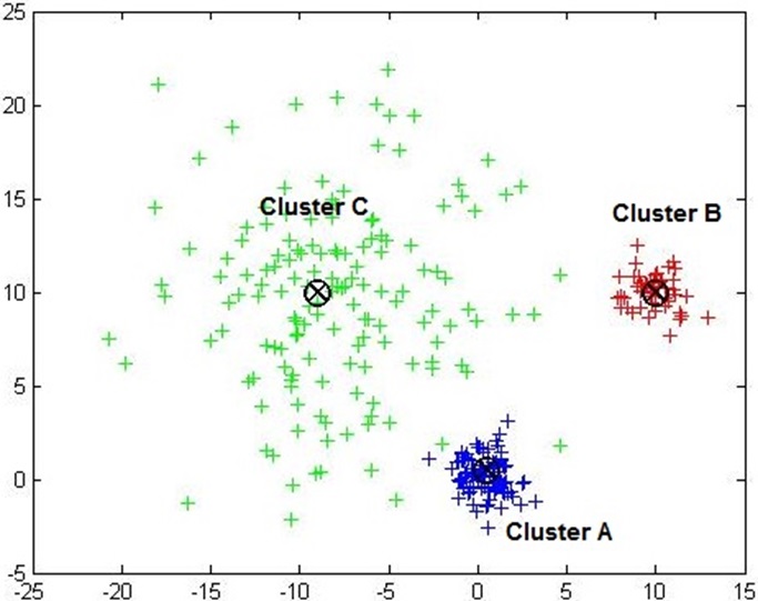
Figure 1: Three clusters generated from Gaussian distributions. Cluster B and C are equally distant to cluster A but cluster C overlaps more with cluster A

3.2.1 Cluster density estimation

Let $x_{1},x_{2},\ldots,x_{N_{i}}$ be the $N_{i}$ features of the $i^{th}$ cluster $C_{i}$.
We assume first that data are generated from multivariate Gaussian distribution given by:

$$p(x|\mu,\Sigma)=\frac{1}{(2\pi)^{d/2}|\Sigma|^{1/2}}exp\left(-\frac{1}{2}(x-\mu)^{T}\Sigma^{-1}(x-\mu)\right)$$ (16)

Where $\mu$ and $\Sigma$ are the mean vector and covariance matrix of the data respectively. T is the transpose operator and $|$ $|$ is the determinant operator. In order to determine the PDF, we need to estimate parameters ($\mu$,$\Sigma$). We apply a maximum likelihood estimation Athanasios (1991) and we obtain the following estimations (see Annex A):

$$\hat{\mu}=\frac{1}{N_{i}}\sum_{i=1}^{N_{i}}x_{i}$$ (17)

$$\hat{\Sigma}=\sum_{i=1}^{N_{i}}(x_{i}-\hat{\mu})^{T}(x_{i}-\hat{\mu})$$ (18)

The Jeffrey divergence between two clusters $C_{i}$ and $C_{j}$ generated from Gaussian distributions $N(\mu_{i},\Sigma_{i})$ and $N(\mu_{j},\Sigma_{j})$ is:

$$JD(C_{i},C_{j}=\frac{1}{2}\left(tr(\Sigma_{i}^{-1}\Sigma_{j})+tr(\Sigma_{j}^{-1}\Sigma_{i})\right)+$$

(19)

To generalize, let us assume that data are generated from any distribution. To estimate the PDF, we rely on the multivariate density distribution using the Gaussian kernel and define the density function as:

$$\hat{p}_{H}(x)=\frac{1}{N_{i}}\sum_{i=1}^{N_{i}}K_{H}(x-x_{i})$$ (20)

Where $H$ is the bandwidth and $K$ is a kernel function:

$$K_{H}(x)=|H|^{-1/2}K(H^{-1/2}x)$$ (21)

We use a Gaussian kernel for the density estimation:

$$K(x)=(2\pi)^{d/2}exp(-\frac{1}{2}x^{T}x)$$ (22)

3.2.2 Separation measure

Based on the computation of Jeffrey divergence, we set up the separation measure as follows: after applying the clustering algorithm, we estimate the density of each cluster $C_{i}$. Divergence between $C_{i}$ and $C_{j,j=,1\ldots,k,j\neq i}$ is computed. After that, we take the minimum of calculated divergences. The separation measure is:

$$S=\sum_{i=1}^{k}Sep_{i}$$ (23)

With:

$$Sep_{i}=\underset{j=1\ldots k,j\neq i}{min}(JD(C_{i},C_{j}))$$ (24)

It is the sum of the minimum of overlap, e.g Jeffrey divergence, between each cluster and other clusters. By choosing the minimum value, we are taking the least overlap degree for each cluster which is an indicator of its separability. A high separation value is an indicator of a good partition.

3.2.3 Compactness measure

The compactness measure is computed as the summation for all clusters of the squared maximal distance of a feature $x_{j}$ belonging to the $i^{th}$ cluster $C_{i}$ to its center $v_{i}$. We denote the compactness measure $V$.

$$V=\sum_{i=1}^{k}\underset{x_{j}\in C_{i}}{max}\left\|x_{j}-v_{i}\right\|^{2}$$ (25)

A low compactness measure indicates a good partition.

3.2.4 Proposed cluster validity index: $I$

The proposed cluster validity index $I$ is the ratio of the proposed separation measure to the compactness measure.

$$I=\frac{V}{S}$$ (26)

A good partition is characterized by a high separation value and a low compactness. Thus, a low value of $I$ is an indicator of a good partition.

4 Experimental results

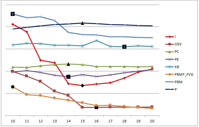
Figure 8: CVIs for S2 with different number of clusters (lines are scaled for display purpose)

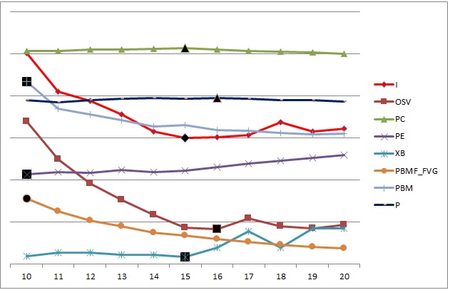
Figure 9: CVIs for S3 with different number of clusters (lines are scaled for display purpose)

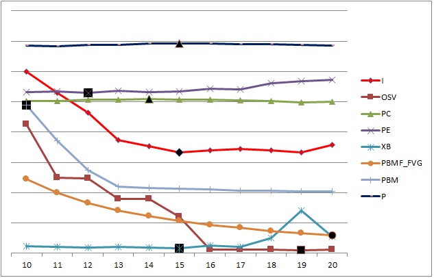
Figure 10: CVIs for S4 with different number of clusters (lines are scaled for display purpose)

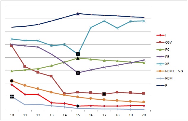
Figure 11: CVIs for R15 with different number of clusters (lines are scaled for display purpose)

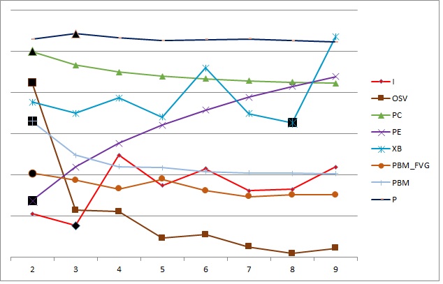
Figure 12: CVIs for Balance data set with different number of clusters (lines are scaled for display purpose)

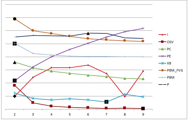
Figure 13: CVIs for Banana data set with different number of clusters (lines are scaled for display purpose)

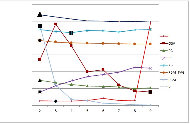
Figure 14: CVIs for Iris data set with different number of clusters (lines are scaled for display purpose)

In order to evaluate the performance of the proposed CVI, we conduct experiments on several synthetic and real data sets with known number of clusters. The classic evaluation methodology consists of applying a clustering algorithm such as FCM on each data set while varying the number of clusters and computing CVIs for each partition. The best CVI determines that the real number of clusters is the one that best fits the data. Figures 7-14 show the variation of each index according to the number of clusters. To evaluate the performances of CVI, we are interested exclusively in checking if the maximum or minimum of each CVI coincides with the optimal number of clusters. The other values of each index are not relevant to this evaluation so curves are scaled for display purposes and the vertical axis has no relevant significance. In addition, for the real data sets, we use a second evaluation method Gurrutxaga et al (2011). In fact, the classic methodology is based on the assumption of the perfection of the clustering algorithm which is not always true. In the alternative methodology, the definition of the best partition is different. Indeed, the best partition is the one which is most similar to the perfect partition. Similarity is quantified using similarity measures such as Rand or adjusted Rand index. The best CVI is the index which determines that the most similar partition to the perfect partition is the best one.
We have computed the proposed measure for clusters of Fig.1; the separation measure between cluster A and B is $Sep_{AB}=69.7$ and between A and C is $Sep_{AC}=22.9$. We can see that the proposed measure reflects better the degree of separation between the three clusters.

4.1 Synthetic data sets

We use four 2-dimensional data sets $S_{1},S_{2},S_{3}$ and $S_{4}$ Fränti and Virmajoki (2006) consisting of 5000 data vectors generated from 15 Gaussian clusters. These data sets are characterized by clusters of different shapes: circular and elliptical. In addition, clusters in data set $S_{1}$ are well separated compared to the other data sets where clusters overlap more and more until becoming indistinguishable in data set $S_{4}$. Furthermore, we use a specially shaped set $R15$ data set Veenman et al (2002). $R15$ consists of 2D 15 Gaussian clusters. Data sets are shown in Figures 2,3, 4, 5 and 6.
We apply FCM with a number of clusters varying from $k=10$ to $k=20$. The CVI which identifies $k=15$ as the best number of cluster is the one that outperforms the others. Results for each set are represented in Fig. 7, 8, 9, 10 and 11. The best result for each CVI is marked in black.
The findings demonstrate that the proposed validity index successfully determines the correct number of clusters for all data sets. On the other hand, indexes such as $PC$ and $PE$ are able to determine the correct number of clusters where there is a low overlapping between clusters such as in data set $S_{1}$. But we can notice that there is a slight variation in their values as overlapping degree gets higher unlike the proposed index $I$ and $XB$ index where discrimination between their values for each number of cluster is obvious. Note that the remaining indexes such PBM and PBMF_FVG completely fail to determine the correct number of clusters in all cases and the best result is always found to be the lowest cluster number.

Figure 2: Data set S1 with 15 Gaussian clusters

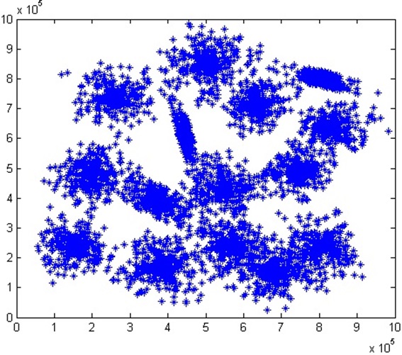
Figure 3: Data set S2 with 15 Gaussian clusters

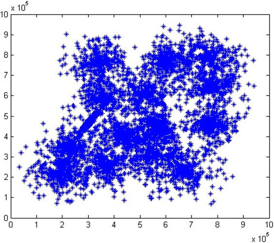
Figure 4: Data set S3 with 15 Gaussian clusters

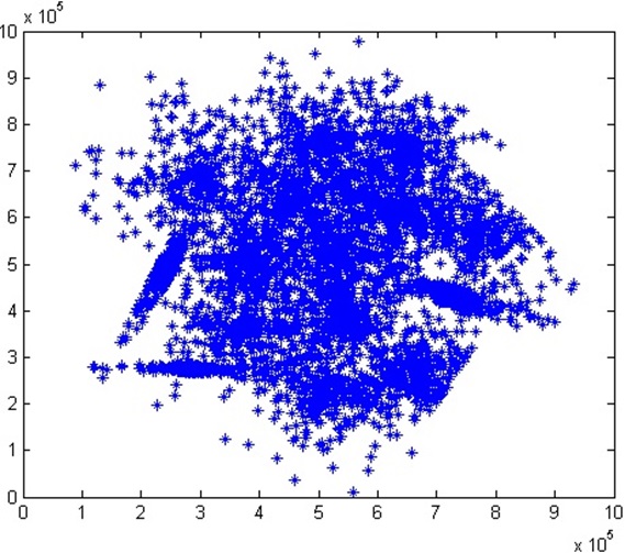
Figure 5: Data set S4 with 15 Gaussian clusters

Figure 6: Data set R15 with 15 Gaussian clusters

4.2 Real data set

4.2.1 Data

• Balance data set Bache and Lichman (2013): This data set represents psychological experimental results. It consists of 625 4D features divided into 3 clusters. Each feature is classified as having balance to the right or to the left or being balanced. The attributes are the left weight, left distance, right weight and right distance.

• Banana data set: This data set is banana shaped. It consists of 5300 features divided into two classes.

• Iris data set Bache and Lichman (2013): Iris is a 4D data set consisting of 150 features divided equally into 3 clusters: Iris setosa, Iris virginica and Iris versicolor. Two of these clusters heavily overlap. The 4D represents sepal length, sepal width, petal length and petal width.

• Extended Yale Database Georghiades et al (2001); Lee et al (2005): This database consists of 16128 images of 28 human subjects under 9 poses and 64 illumination conditions. In our experiments, we use the first 5 and 7 classes data with 64 images each denoted Yale_5 and Yale_7 respectively. We resize the cropped images into $24\times 21$ then project the data onto a lower dimensional subspace using PCA.

• Hopkins 155: This data set consists of 156 sequences of two and three motions which can be devided into three categories: checkerkboard, traffic and articulated sequences. Each sequence is a segmentation task. The checkerboard category consists of 104 sequences of indoor scenes taken with a handheld camera under controlled conditions. The checkerboard pattern on the objects is used to assure a large number of tracked points. Traffic category consists of 38 sequences of outdoor traffic scenes taken by a moving handheld camera. Articulated sequences display motions constrained by joints, head and face motions, people walking, etc.

4.2.2 Classic methodology: results

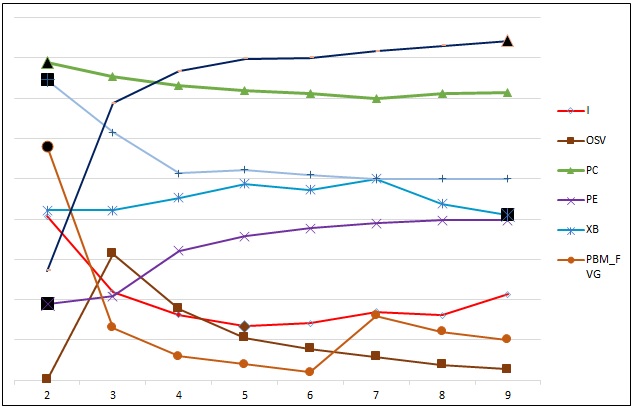
Figure 15: CVIs for Yale_5 data set with different number of clusters (lines are scaled for display purpose)

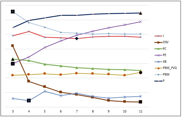
Figure 16: CVIs for Yale_7 with different number of clusters (lines are scaled for display purpose)

Results in Fig. 12 for Balance data set demonstrate that only the proposed index and the $P$ index are able to determine the optimal number of clusters. The behavior of indexes such as PC and PBM_FVG seen with synthetic data sets is confirmed with the real data set, i.e the lowest number of clusters is chosen as the optimal number. These indexes represent a monotonic tendency with the number of clusters.
In Fig. 13 for Banana data set, the proposed validity index estimated that the real number of cluster e.g $c^{*}=2$ is the optimal number of cluster. A large variation in index $I$ is noticed. This gives an information about the correct number of cluster. Almost all the validity indexes were able to estimate $c^{*}$. The monotonic tendency of some indexes such as $PE$ and $PC$ is also confirmed.
The presence of overlap in the Iris data set makes it difficult to estimate the optimal number of cluster. Only index $I$ was able to determine $c^{*}=3$ as the optimal number of clusters as shown in Fig. 14. $PC$ and $PE$ always exhibit the monotonic tendency for the number of clusters. $PBM$ and $PBMF\_FVG$ showed the same behavior as for the previous data sets.
With eYale database, index I exhibits good performance. Indeed, for Yale_5 data set as showeed in Fig. 15, only the proposed index was able to predict the real number of cluster as well as for Yale_7 data set according to the results in Fig. 16.

4.2.3 Alternative methodology: results

We use four similarity measures namely the Rand index, the Fowlkes-Mallows (FM), the Jaccard (Jacc) and the adjsuted Rand (ARI) indexes Jain and Dubes (1988) which are described in Appendix C. We run FCM 100 times on the selected data and compute how many times each CVI determines the most similar partition as the best partition. Results for Balance, Banana and Iris are shown in tables 1, 2 and 3.
For the balance data set, index $I$ presents good performance. In fact, it is able to detect the best partition for all the similarity measures unlike other indexes which perform well with some similarity measures but fail with others such as PC and PE known for their monotonic tendency.
For the banana data set, the proposed index also presents good performances. It was able to determine the optimal partition with all similarity measures except Rand.
For Iris data set, only the proposed index $I$ was able to determine the best partition in case of Rand, Jaccard and adjusted Rand indexes. Such result goes with the result obtained for Iris data in the classic methodology.
For the Hopkins 155 data, we use the 1R2RCT_A, 1R2RCT_B and car5 data sets which have three motions each. A classic preprocessing step before using these data is to project it onto a subspace using PCA. In fact, it is known for these data that the feature trajectories of $n$ motions in a video almost perfectly lie in a $4n$ dimensional subspace. Thus, PCA projection will reduce the dimensionality with structure preservation Elhamifar and Vidal (2013). Results are shown in tables 4, 5 and 6. The overall performance of the proposed index is better than the other indexes for 1R2RCT_A for all the similarity measures except ARI. Other indexes completely fail with Rand, FM and Jacc measures. With 1R2RT_B, index I presents also good performance with a success of 100% for Rand, FM and Jacc. PC and XB in this case present also the same performance. OSV and P perform well only with ARI. Results for car5 demonstrate also the outperformance of index I with Rand FM and ARI. In general, results on Hopkins 155 demonstrate that the proposed index I presents the best success rate compared to other indexes.

4.3 Discussion

The proposed validity index is highly useful especially for data sets where overlap between clusters is present. While some indexes are robust or completely fail in the presence of a low degree of overlapping, proposed index $I$ is robust and able to estimate the optimal number of cluster even when clusters highly overlap such as in data sets $Iris$ and $S_{4}$ data sets where all or some clusters are hardly distinguishable. The design of the separation measure based on the density of clusters is an indicator of the degree of overlap between clusters as shown in section 4 which couldn’t be determined with the classical separation measure based on the distance between cluster centers. However, in case of high dimensional data, the computation of the proposed cluster validity index may be computationally expensive. For example, in case of Gaussian clusters, the computation of Jeffrey divergence (27) requires the inversion of the covariance matrix of size ($d\times d$). Using Cholesky decomposition, this operation has a complexity of $O(d^{3})$.

5 Conclusion

Cluster validity indexes are used to compare the performances of clustering algorithms and determine the optimal number of clusters that best fits the data. Most of CVIs available in the literature use a separation measure based on distance computation between cluster centers. It has been proven that such measure is not efficient especially in the case of overlapping clusters where it gives misleading results.
In this work, we proposed a new cluster validity index based on a new separation measure. The optimal partition is obtained with the lowest value of the index which means a high separation and low compactness. The proposed separation measure, unlike the classic ones, is based on density estimation of the obtained clusters. Jeffrey divergence is computed afterward informing us about the degree of overlap between pairs of clusters. The experimentation involved synthetic and real data sets. Comparisons between the proposed CVI and other CVIs have been conducted. Results demonstrated that the proposed CVI outperforms other indexes especially in the case of a data set containing overlapping clusters. In a future work, we will attempt to incorporate a local adaptive distance in the design of the CVI. This adaptive approach is expected to give significant separation and compactness measures.

Aknowledgment

This publication was made possible by NPRP grant # 4-1165- 2-453 from the Qatar National Research Fund (a member of Qatar Foundation). The statements made herein are solely the responsibility of the authors.

Figure 7: CVIs for S1 with different number of clusters (lines are scaled for display purpose)

Table 1: Similarity measures for balance data set

Similarity	PC	PE	P	XB	PBM	PBM	OSV	I
measure						_FVG
Rand	0	0	0	0	0	0	75	9
FM	100	100	0	0	100	100	0	69
Jacc	100	100	0	0	100	100	0	67
ARI	0	0	0	0	0	0	79	11

Table 2: Similarity measures for banana data set

Similarity	PC	PE	P	XB	PBM	PBM	OSV	I
measure						_FVG
Rand	0	81	8	58	0	0	29	0
FM	100	100	0	0	100	100	0	100
Jacc	100	100	0	0	100	100	0	100
ARI	100	0	0	0	0	0	0	100

Table 3: Similarity measures for Iris data set

Similarity	PC	PE	P	XB	PBM	PBM	OSV	I
measure						_FVG
Rand	0	0	0	0	0	0	0	17
FM	100	100	0	100	100	100	0	0
Jacc	0	0	0	0	0	0	0	15
ARI	0	0	0	0	0	0	0	84

Table 4: Similarity measures for 1R2RCT_A data set

Similarity	PC	PE	P	XB	PBM	PBM	OSV	I
measure						_FVG
Rand	0	0	0	0	0	0	0	80
FM	0	0	0	0	0	0	0	80
Jacc	0	0	0	0	0	0	0	80
ARI	100	100	0	0	100	100	0	0

Table 5: Similarity measures for 1R2RT_B data set

Similarity	PC	PE	P	XB	PBM	PBM	OSV	I
measure						_FVG
Rand	100	0	0	100	0	0	0	100
FM	100	0	0	100	0	0	0	100
Jacc	100	0	0	100	0	0	0	100
ARI	0	100	90	0	0	0	66	0

Table 6: Similarity measures for car5 data set

Similarity	PC	PE	P	XB	PBM	PBM	OSV	I
measure						_FVG
Rand	0	0	0	76	0	0	0	96
FM	41	41	0	61	0	41	41	82
Jacc	99	99	0	0	0	99	99	0
ARI	0	0	0	0	76	0	0	96

Annex A. Parameters estimation

In all the expressions below, x is a vector of random variables whose mean vector and covariance matrix are given by: $E(x)=\mu$ and $E((x-\mu)(x-\mu)^{T})=\Sigma$ where $E$ means the expectation. Using matrix properties:

• $\frac{\partial A^{T}\cdot x}{\partial x}=\frac{\partial x^{T}\cdot A}{\partial x}=A$

• $\frac{\partial x^{T}\cdot A\cdot x}{\partial x}=A^{T}+A$

• $\frac{\partial}{\partial A}log|A|=\left(A^{-1}\right)^{T}$

• $\frac{\partial}{\partial A}tr\left[AB\right]=tr\left[BA\right]=B^{T}$

The log likelihood of the multivariate Gaussian distribution is given by:

$$L(x|\mu,\Sigma)=\frac{-nD}{2}log(2\pi)-\frac{n}{2}log(|\Sigma|)-$$

(27)

The estimates of the mean and covariance matrix are determined by computing the derivatives of $L(x|\mu,\Sigma)$ with relative to $\mu$ and $\Sigma$ and set it equal to zero.

$$\frac{\partial L(x|\mu,\Sigma)}{\partial\mu}$$

$$\frac{\partial L(x|\mu,\Sigma)}{\partial\Sigma^{-1}}$$

Annex B. Jeffrey divergence for multivariate Gaussian distribution

We use the following formula:

• $E(x^{T}\cdot A\cdot x)=tr(A\cdot\Sigma)+\mu^{T}\cdot A\cdot\mu$

• $\left\langle\cdot\right\rangle$ is the expectation symbol.

$$p(x|\mu_{1},\Sigma_{1})=\frac{1}{(2\pi)^{d/2}|\Sigma_{1}|^{1/2}}exp\left(-\frac{1}{2}(x-\mu_{1})^{T}\Sigma_{1}^{-1}(x-\mu_{1})\right)$$

$$q(x|\mu_{2},\Sigma_{2})=\frac{1}{(2\pi)^{d/2}|\Sigma_{2}|^{1/2}}exp\left(-\frac{1}{2}(x-\mu_{2})^{T}\Sigma_{2}^{-1}(x-\mu_{2})\right)$$

$$JD(p,q)=KL(p/q)+KL(q/p)$$

Where $KL$ is the Kullback-Leiber divergence.

$$KL(p/q)$$

Thus:

$$JD(p,q)$$

Annex C. Similarity measures

The four similarity measures we have used are described in this section. Let $P1$ and $P2$ two partitions. We define $a$ as the number of object pairs that belong to the same clusters in both $P1$ and $P2$. Let $b$ be the number of object pairs that belongs to different clusters in both pairs. Let $c$ be the number of object pairs that belong to the same clusters in $P1$ but in different clusters in $P2$. Finally, let $d$ the number of pairs that belong to different clusters in $P1$ but belong to the same cluster in $P2$. The four similarity measures are defined as:

$$Rand$$

$$Fowlkes-Mallows$$

$$Jaccard$$

$$Adjsuted-Rand$$

References

- Arbelaitz et al (2013) Arbelaitz O, Gurrutxaga I, Muguerza J, Pérez JM, Perona I (2013) An extensive comparative study of cluster validity indices. Pattern Recognition 46(1):243–256
- Athanasios (1991) Athanasios P (1991) Probability, Random Variables and Stochastic Processes, 3rd edn. McGraw-Hill Companies
- Bache and Lichman (2013) Bache K, Lichman M (2013) UCI machine learning repository. URL http://archive.ics.uci.edu/ml
- Bandyopadhyay et al (2011) Bandyopadhyay S, Saha S, Pedrycz W (2011) Use of a fuzzy granulation-degranulation criterion for assessing cluster validity. Fuzzy Sets and Systems 170:22 – 42
- Bezdek (1974) Bezdek JC (1974) Cluster validity with fuzzy sets. Journal of Cybernetics 3:58–73
- Bezdek (1981) Bezdek JC (1981) Pattern Recognition with Fuzzy Objective Function Algorithms. Plenum Press. New York and London
- Chang et al (2009) Chang H, Yao Y, Koschan A, Abidi B, Abidi M (2009) Improving face recognition via narrowband spectral range selection using jeffrey divergence. Information Forensics and Security, IEEE Transactions on 4(1):111–122
- Chen and Linkens (2004) Chen MY, Linkens D (2004) Rule-base self-generation and simplification for data-driven fuzzy models. Fuzzy Sets and Systems 142:243–265
- Deza et al (2009) Deza, Marie M, Deza, Elena (2009) Encyclopedia of Distances. Springer Heidelberg New York Dordrecht London
- Elhamifar and Vidal (2013) Elhamifar E, Vidal R (2013) Sparse subspace clustering: Algorithm, theory, and applications. Pattern Analysis and Machine Intelligence, IEEE Transactions on 35(11):2765–2781
- Ester et al (1996) Ester M, peter Kriegel H, S J, Xu X (1996) A density-based algorithm for discovering clusters in large spatial databases with noise. AAAI Press, pp 226–231
- Everitt et al (2011) Everitt BS, Landau S, Leese M, Stahl D (2011) An Introduction to Classification and Clustering, John Wiley & Sons, Ltd, chap 1, pp 1–13
- Fränti and Virmajoki (2006) Fränti P, Virmajoki O (2006) Iterative shrinking method for clustering problems. Pattern Recognition 39(5):761 – 775
- Georghiades et al (2001) Georghiades A, Belhumeur P, Kriegman D (2001) From few to many: Illumination cone models for face recognition under variable lighting and pose. IEEE Trans Pattern Anal Mach Intelligence 23(6):643–660
- Gurrutxaga et al (2011) Gurrutxaga I, Muguerza J, Arbelaitz O, Pérez JM, Martín JI (2011) Towards a standard methodology to evaluate internal cluster validity indices. Pattern Recognition Letters 32:505–515
- Jain and Dubes (1988) Jain A, Dubes R (1988) Algorithms for Clustering Data. Prentice-Hall Englewood Cliffs, New York
- Jain (2010) Jain AK (2010) Data clustering: 50 years beyond k-means. Pattern Recognition Letters 31:651 – 666
- Krooshof et al (2012) Krooshof PW, Postma GJ, Melssen WJ, Buydens LM (2012) Biomedical Imaging: Principles and Applications, John Wiley & Sons, Inc., chap 12, pp 1–29
- Lee et al (2005) Lee K, Ho J, Kriegman D (2005) Acquiring linear subspaces for face recognition under variable lighting. IEEE Trans Pattern Anal Mach Intelligence 27(5):684–698
- Mu et al (2013) Mu Y, Ding W, Tao D (2013) Local discriminative distance metrics ensemble learning. Pattern Recognition 46(8):2337 – 2349
- Pakhira et al (2004) Pakhira MK, Bandyopadhyay S, Maulik U (2004) Validity index for crisp and fuzzy clusters. Pattern Recognition 37:487 – 501
- Pakhira et al (2005) Pakhira MK, Bandyopadhyay S, Maulik U (2005) A study of some fuzzy cluster validity indices, genetic clustering and application to pixel classification. Fuzzy Sets and Systems 155:191–214
- Pascual et al (2010) Pascual D, Pla F, Sأ،nchez JS (2010) Cluster validation using information stability measures. Pattern Recognition Letters 31(6):454 – 461
- Puzicha et al (1997) Puzicha J, Hofmann T, Buhmann J (1997) Non-parametric similarity measures for unsupervised texture segmentation and image retrieval. In: Proceedings of IEEE Conference on Computer Vision and Pattern Recognition, 1997, pp 267–272
- Sugiyama (2007) Sugiyama M (2007) Dimensionality reduction of multimodal labeled data by local fisher discriminant analysis. J Mach Learn Res 8:1027–1061
- Tran et al (2005) Tran TN, Wehrens R, Buydens LM (2005) Clustering multispectral images: a tutorial. Chemometrics and Intelligent Laboratory Systems 77:3–17
- Veenman et al (2002) Veenman CJ, Reinders M, Backer E (2002) A maximum variance cluster algorithm. IEEE Transactions on Pattern Analysis and Machine Intelligence 24:1273–1280
- Žalik (2010) Žalik KR (2010) Cluster validity index for estimation of fuzzy clusters of different sizes and densities. Pattern Recognition 43(10):3374–3390
- Žalik and Žalik (2011) Žalik KR, Žalik B (2011) Validity index for clusters of different sizes and densities. Pattern Recognition Letters 32:221–234
- Wang and Zhang (2007) Wang W, Zhang Y (2007) On fuzzy cluster validity indices. Fuzzy Sets and Systems 158:2095–2117
- Weinberger et al (2006) Weinberger KQ, Blitzer J, Saul LK (2006) Distance metric learning for large margin nearest neighbor classification. In: In NIPS, MIT Press
- Wu et al (2009) Wu KL, Yang MS, Hsieh JN (2009) Robust cluster validity indexes. Pattern Recognition 42(11):2541–2550
- Xie and Beni (1991) Xie XL, Beni G (1991) A validity measure for fuzzy clustering. IEEE Transactions on Pattern Analysis and Machine Intelligence 13:841–847
- Xing et al (2003) Xing EP, Ng AY, Jordan MI, Russell S (2003) Distance metric learning, with application to clustering with side-information. In: Advances in Neural Information Processing systems 15, MIT Press, pp 505–512
- Zheng and You (2013) Zheng J, You H (2013) A new model-independent method for change detection in multitemporal sar images based on radon transform and jeffrey divergence. Geoscience and Remote Sensing Letters, IEEE 10(1):91–95