The symmetries of octupolar tensors

Abstract

Octupolar tensors are third order, completely symmetric and traceless tensors. Whereas in 2D an octupolar tensor has the same symmetries as an equilateral triangle and can ultimately be identified with a vector in the plane, the symmetries that it enjoys in 3D are quite different, and only exceptionally reduce to those of a regular tetrahedron. By use of the octupolar potential that is, the cubic form associated on the unit sphere with an octupolar tensor, we shall classify all inequivalent octupolar symmetries. This is a mathematical study which also reviews and incorporates some previous, less systematic attempts.

1 Introduction

It is well known that the Landau theory of phase transitions landau:theory ; landau:theory_I ; LL ; Peliti ; Toledano describes the states of matter in the vicinity of a critical point in terms of an order parameter; in the simplest cases this is a scalar quantity, but it can be a vector, or more generally a tensor of any order.

In fact, in the case of liquid crystals it is rather common to describe their state in terms of a second-order tensor PdG ; GLJ ; VirgaBook . More recently, it became apparent that certain materials displaying tetrahedral nematic phases Fel1 ; Fel2 are better described in terms of a third order tensor $\mathbf{A}$ – more precisely, a fully symmetric and completely traceless one (see below for definitions). We stress that it is conceivable, even probable, that order parameters described by still higher order tensors will be needed in considering generalized liquid crystals liu:classification ; liu:generalized ; liu:generic .

This is precisely what is meant in this paper by an octupolar tensor: a third order, fully symmetric and completely traceless tensor. Although, as also shown below, octupolar tensors feature in many branches of physics, we shall systematically use the paradigm of the Landau theory of phase transitions to illustrate the physical significance of our study. The reader is advised from the start that this is but one of many incarnations of our mathematical theory, which is concerned with the symmetries of the most general octupolar tensor in three space dimensions.

One of us provided a complete description of the physics of a material represented by an octupolr tensor in the two dimensional case Virga2D . In this case, one obtains a remarkably simple description, and the physical state is basically identified by the orientation of an equilateral triangle in the order parameter space.

Unfortunately, such a simple description is peculiar to the 2D case, and as soon as we pass to consider a three-dimensional situation things become much more involved. In a recent contribution GV2016 (see also CQV ), we have studied this situation, providing a description of the physics described by an octupolar tensor in three dimensions; this study also showed an unexpected feature awaiting experimental confirmation, i.e. the existence – together with higher symmetric special phases – of two different generic phases; the interface between these has been investigated in detail in a subsequent work CQV .

In our efforts to classify all symmetries of an octupolar tensor $\mathbf{A}$ a prominent role is played by the appropriate notion of eigenvalues and eigenvectors applicable for ${\bf A}$. In multilinear algebra, such a notion is not as univocally defined as one might naively think. For real-valued tensors that bear a physical meaning, as the ones we are interested in, the issue arises as to whether complex eigenvalues, which would perfectly be allowed according to certain definitions, should be admitted or not. The definition of eigenvalues (and associated eigenvectors) that we adopt in this paper is essentially the one put forward in qi:eigenvalues ; qi:rank ; qi:eigenvalues_invariants (see also the recent book qi:tensor , especially Chap. 7, which is specifically concerned with octupolar tensors and their mechanical applications). However, we give an equivalent characterization of this notion in terms of the critical points of a cubic polynomial defined over the unit sphere $S^{2}$. This is indeed the natural extension of what one learns from the lucid (and now rare) book of Noll noll:finite-dimensional . In Sect. 84, the maximum and minimum of the spectrum of a symmetric, second order tensor $\mathbf{S}$ in a $n$-dimensional space are characterized as the corresponding extrema of the quadratic form associated with $\mathbf{S}$ on the unit sphere $S^{n-1}$. Noll’s book was published in 1987, but its contents were available many years back.

In our previous work GV2016 we focused on the physics of the problem, and in particular of its generic phases – discovering an unexpected phenomenon, i.e. the existence of two generic (octupolar) phases, hence the possibility of an intra-octupolar phase transition (see also CQV for details on this) – providing little mathematical detail; the purpose of the present paper is twofold:

1. On the one hand, we want to give a full account of the mathematical details needed for the study of such a problem. We trust that – beside the interest per se – this will also be relevant to systems described by higher order tensors liu:classification ; liu:generalized ; liu:generic .

2. On the other hand, also thanks to this higher mathematical detail provided here, we want to discuss in more detail the non-generic phases (and the transitions between these), thus completing the physical description provided in previous work GV2016 ; CQV .

The plan of the paper is as follows. In Sect. 2 we present the physical motivation of our work; in Sect. 3 we discuss the general features of a prototypical Landau potential, which will be referred to as the octupolar potential, for short. As this potential is based on octupolar tensors in three spatial dimensions, the subsequent Sect. 4 is devoted to study these objects and their eigenvectors. We can then pass, in Sect. 5, to study the general octupolar potential; this depends a priori on seven parameters, but by a suitable choice of reference frame and of the potential scale – as discussed in Sect. 5 – we can reduce to study a problem depending only on three parameters; the allowed parameters are described by a cylinder in parameter space. It turns out that this potential and its critical points bear some relation to the tetrahedral group; Sect. 6 is thus devoted to recalling some basic facts about this. We can then pass to study the extremals of the Landau potential; these depend of course on the parameters and different regions in the allowed cylinder in parameter space correspond actually to different symmetries (phases) for the potential and its critical set, as discussed in detail in Sect. 7 and its subsections, each devoted to one of these phases. Finally in Sect. 8 we review and summarize our findings, with special emphasis on the distribution in parameter space of the critical points of the octupolar potential. In the final Sect. 9 we draw our conclusions. The paper is completed by an appendix with details on the tetrahedral group beyond the brief discussion of Sect. 6.

Whenever indices are needed, summation over repeated pairs will be routinely understood, unless explicitly stated otherwise.

2 Physical motivation

Octupolar tensors have many manifestations in physics. In this section, we shall review a few of them, ranging from the most classical to the most innovative ones.

Among the former is Buckingham’s formula Buck for the probability density $\varrho$ of the the distribution of a molecular director $\bm{\ell}$ over the unit sphere $S^{2}$, which can be written as

$$\varrho(\bm{\ell})=\frac{1}{4\pi}\left(1\ +\sum_{k=1}^{\infty}\frac{(2k+1)!!}{k!}\left\langle\mbox{$\hskip 1.99997pt\stackrel{{\scriptstyle\mbox{$\vphantom{\rule[-2.58316pt]{0.51663pt}{3.0998pt}}\rule[-2.06653pt]{0.51663pt}{2.58316pt}\rule{11.61392pt}{0.51663pt}\rule[-2.06653pt]{0.51663pt}{2.58316pt}$}}}{{\mbox{$\displaystyle{\bm{\ell}^{\otimes k}}$}}}\hskip 1.99997pt$}\right\rangle_{\!\!\!\varrho}\cdot\bm{\ell}^{\otimes k}\right),$$ (1)

where, for a generic vector ${\mathbf{x}}$, ${\bf x}^{\otimes k}$ is the $k$th-order tensor defined as in turzi:cartesian by

$${\bf x}^{\otimes k}={\bf x}\otimes...\otimes{\bf x}$$ (2)

(with $k$ factors, of course), $\cdot$ denotes tensor contraction, and $\left\langle\mbox{$\hskip 1.99997pt\stackrel{{\scriptstyle\mbox{$\vphantom{\rule[-2.58316pt]{0.51663pt}{3.0998pt}}\rule[-2.06653pt]{0.51663pt}{2.58316pt}\rule{6.80557pt}{0.51663pt}\rule[-2.06653pt]{0.51663pt}{2.58316pt}$}}}{{\mbox{$\displaystyle{\bf P}$}}}\hskip 1.99997pt$}\right\rangle_{\!\!\!\varrho}$ is the multipole average,

$$\left\langle\mbox{$\hskip 1.99997pt\stackrel{{\scriptstyle\mbox{$\vphantom{\rule[-2.58316pt]{0.51663pt}{3.0998pt}}\rule[-2.06653pt]{0.51663pt}{2.58316pt}\rule{6.80557pt}{0.51663pt}\rule[-2.06653pt]{0.51663pt}{2.58316pt}$}}}{{\mbox{$\displaystyle{\bf P}$}}}\hskip 1.99997pt$}\right\rangle_{\!\!\!\varrho}:=\frac{1}{4\pi}\int_{S^{2}}\left\langle\mbox{$\hskip 1.99997pt\stackrel{{\scriptstyle\mbox{$\vphantom{\rule[-2.58316pt]{0.51663pt}{3.0998pt}}\rule[-2.06653pt]{0.51663pt}{2.58316pt}\rule{6.80557pt}{0.51663pt}\rule[-2.06653pt]{0.51663pt}{2.58316pt}$}}}{{\mbox{$\displaystyle{\bf P}$}}}\hskip 1.99997pt$}\right\rangle\varrho({\bm{\ell}})\mathrm{d}\bm{\ell},$$ (3)

of the symmetric, traceless part $\hskip 1.99997pt\stackrel{{\scriptstyle\mbox{$\vphantom{\rule[-2.58316pt]{0.51663pt}{3.0998pt}}\rule[-2.06653pt]{0.51663pt}{2.58316pt}\rule{6.80557pt}{0.51663pt}\rule[-2.06653pt]{0.51663pt}{2.58316pt}$}}}{{\mbox{$\displaystyle\bf P$}}}\hskip 1.99997pt$ of a tensor ${\bf P}$.

With this notation, our octupolar order tensor ${\bf A}$ is identified with

$${\bf A}=\left\langle\mbox{$\hskip 1.99997pt\stackrel{{\scriptstyle\mbox{$\vphantom{\rule[-2.58316pt]{0.51663pt}{3.0998pt}}\rule[-2.06653pt]{0.51663pt}{2.58316pt}\rule{28.05566pt}{0.51663pt}\rule[-2.06653pt]{0.51663pt}{2.58316pt}$}}}{{\mbox{$\displaystyle{\bm{\ell}\otimes\bm{\ell}\otimes\bm{\ell}}$}}}\hskip 1.99997pt$}\right\rangle_{\!\!\!\varrho}.$$ (4)

Passing to spherical coordinates, and writing $\bm{\ell}$ as

$${\bm{\ell}}=\sin\vartheta\cos\varphi\,\mathbf{e}_{1}+\sin\vartheta\sin\varphi\,\mathbf{e}_{2}+\cos\vartheta\,\mathbf{e}_{3},$$ (5)

we easily express the scalar parameters that represent ${\bf A}$ in the Cartesian frame $(\mathbf{e}_{1},\mathbf{e}_{2},\mathbf{e}_{3})$ in terms of multipole averages, which also reveal the bounds they are subject to GV2016 .

In nonlinear optics (see, for example Sect. 1.5 of boyd:nonlinear , and also zyss:nonlinear and kanis:design ), higher order susceptibilities tensors, often called hypersusceptibilities (and also hyperpolarizabilities), are introduced to decompose the electromagnetic energy density in multipoles. In particular, the cubic term has the general form

$$U^{(2)}=\chi^{(2)}_{ijk}F_{i}F_{j}F_{k},$$ (6)

where $F_{i}$ are the components of an external field and $\chi^{(2)}_{ijk}$ are the components of the first hypersusceptibility tensor $\bm{\chi}^{(2)}$, which is a third order tensor.

When the frequencies of the applied fields are much smaller than the resonance frequency, $\bm{\chi}^{(2)}$ can safely be assumed to be independent of frequencies and fully symmetric in all its indices. Though this symmetry, which is often called Kleinman’s symmetry after the name of the author who first introduced it kleinman:nonlinear , has been widely criticized dailey:general and also found in disagreement with some computational schemes wergifosse:evaluation , it is still often accepted as an approximation for its simplicity. Assuming Kleinman’s symmetry to be valid, we can extract an octupolar tensor ${\bf A}=\mbox{$\hskip 1.99997pt\stackrel{{\scriptstyle\mbox{$\vphantom{\rule[-2.58316pt]{0.51663pt}{3.0998pt}}\rule[-2.06653pt]{0.51663pt}{2.58316pt}\rule{13.41248pt}{0.51663pt}\rule[-2.06653pt]{0.51663pt}{2.58316pt}$}}}{{\mbox{$\displaystyle\bm{\chi}^{(2)}$}}}\hskip 1.99997pt$}$ out of $\bm{\chi}^{(2)}$ and rewrite the latter in the equivalent form

$$\chi^{(2)}_{ijk}=A_{ijk}+\frac{1}{5}\left(\chi^{(2)}_{i}\delta_{jk}+\chi^{(2)}_{j}\delta_{ki}+\chi^{(2)}_{k}\delta_{ij}\right),$$ (7)

where $\chi^{(2)}_{k}:=\chi^{(2)}_{iik}=\chi^{(2)}_{iki}=\chi^{(2)}_{kii}$. Using (7) in (6), we also write

$$U^{(2)}=A_{ijk}F_{i}F_{j}F_{k}+\frac{3}{5}F^{2}\chi^{(2)}_{i}F_{i},$$ (8)

where $F$ is the strength of the applied field. Normalizing $F$ to unity, $U^{(2)}$ becomes the sum of an octupolar and a dipolar potential, the latter of which contributes to a lower multipole.

A third order tensor very similar to $\bm{\chi}^{(2)}$ was introduced in lubensky:theory to describe the ordering of bent-core molecules that possess liquid crystal phases. As also recalled in CQV , the theory of bent-core liquid crystal phases features a mesoscopic third order tensor derived from $\hskip 1.99997pt\stackrel{{\scriptstyle\mbox{$\vphantom{\rule[-2.58316pt]{0.51663pt}{3.0998pt}}\rule[-2.06653pt]{0.51663pt}{2.58316pt}\rule{13.55258pt}{0.51663pt}\rule[-2.06653pt]{0.51663pt}{2.58316pt}$}}}{{\mbox{$\displaystyle\bm{\alpha}^{(3)}$}}}\hskip 1.99997pt$; here $\bm{\alpha}^{(3)}$ is the molecular structural tensor defined by

$$\bm{\alpha}^{(3)}:=\sum_{\mu=1}^{N}m_{\mu}\mathbf{r}_{\mu}\otimes\mathbf{r}_{\mu}\otimes\mathbf{r}_{\mu},$$ (9)

where the sum is extended to all the atoms in a constituent molecule, $m_{\mu}$ is the mass of each individual atom and $\mathbf{r}_{\mu}$ is its position vector relative to the molecule’s center of mass. The ensemble average ${\bf A}=\left\langle\mbox{$\hskip 1.99997pt\stackrel{{\scriptstyle\mbox{$\vphantom{\rule[-2.58316pt]{0.51663pt}{3.0998pt}}\rule[-2.06653pt]{0.51663pt}{2.58316pt}\rule{13.55258pt}{0.51663pt}\rule[-2.06653pt]{0.51663pt}{2.58316pt}$}}}{{\mbox{$\displaystyle{\bm{\alpha}^{(3)}}$}}}\hskip 1.99997pt$}\right\rangle$ is an octupolar tensor that plays an important role in classifying all possible new phases that bent-core liquid crystals are allowed to exhibit. They have been collectedly called tetrahedral by a symmetry that ${\bf A}$ can indeed enjoy, but our study has shown to be only too special, rather than generic.

Lately, octupolar tensors have also become popular with the classical elastic theory of nematic liquid crystals (both passive and active). The nematic director field $\mathbf{n}$ represents at the macroscopic scale the average orientation of the elongated molecules that constitute the medium. Elastic distortions of $\mathbf{n}$ are measured locally by its spatial gradient $\nabla\mathbf{n}$, which may become singular at certain points in space in response to external distorting stimuli. These are the defects of $\mathbf{n}$, where molecular order is degraded; they can be classified into distinct topological classes, associated in 2D with the winding number $m$ of $\mathbf{n}$ around a point defect ($m$, which is often referred to as the topological charge, is half an integer; more information about defects in liquid crystals and their topological charges can be obtained from the monographs stewart:static and VirgaBook ).

It has recently been proposed vromans:orientational that a vector be associated with a point defect in 2D to represent the average direction along which the field $\mathbf{n}$ is fluted away from the defect. It is believed that such a vector could play a role in describing the interaction of defects, as if they were oriented particles interacting like vessels in a viscous sea. If this image is indeed suggestive for the charge $m=\frac{1}{2}$, when the integral lines of $\mathbf{n}$ around the defect resemble a flame, associating a single direction with a defect with charge $m=-\frac{1}{2}$ seems somehow troublesome at first sight, as in that case the integral lines of $\mathbf{n}$ escape along three directions, ideally separating the plane in three equal sectors. To overcome this difficulty, it has been proposed in tang:orientation to describe the orientation of a $-\frac{1}{2}$ defect through the octupolar tensor

$${\bf A}=\left\langle\mbox{$\hskip 1.99997pt\stackrel{{\scriptstyle\mbox{$\vphantom{\rule[-2.58316pt]{0.51663pt}{3.0998pt}}\rule[-2.06653pt]{0.51663pt}{2.58316pt}\rule{27.2223pt}{0.51663pt}\rule[-2.06653pt]{0.51663pt}{2.58316pt}$}}}{{\mbox{$\displaystyle{\nabla\mathbf{n}\otimes\mathbf{n}}$}}}\hskip 1.99997pt$}\right\rangle,$$ (10)

where the average $\left\langle{\cdots}\right\rangle$ is now meant to be computed on a sufficiently small neighborhood surrounding the defect. As shown in Virga2D , any octupolar tensor ${\bf A}$ in 2D possesses the symmetries of an equilateral triangle, and its most general representation is given by

$${\bf A}=\alpha\mbox{$\hskip 1.99997pt\stackrel{{\scriptstyle\mbox{$\vphantom{\rule[-2.58316pt]{0.51663pt}{3.0998pt}}\rule[-2.06653pt]{0.51663pt}{2.58316pt}\rule{28.88893pt}{0.51663pt}\rule[-2.06653pt]{0.51663pt}{2.58316pt}$}}}{{\mbox{$\displaystyle\mathbf{e}\otimes\mathbf{e}\otimes\mathbf{e}$}}}\hskip 1.99997pt$},$$ (11)

where $\alpha$ is a scalar and $\mathbf{e}$ is a unit vector in in the plane. Thus, in 2D, ${\bf A}$ effectively reduces to a vector and both approaches in vromans:orientational and tang:orientation are equivalent. However, as shown in GV2016 , in 3D ${\bf A}$ cannot in general be represented in terms of a single vector as in (11) and (10) becomes a more versatile tool to describe the directions along which the integral lines of $\mathbf{n}$ are fluted around a point defect. In particular, it might be interesting to compute ${\bf A}$ in (10) for the combed defects described in saupe:disclinations and their distortions possibly due to the interaction with other point defects nearby (see also sonnet:reorientational ). The complete classification of the symmetries enjoyed by ${\bf A}$, which we give in this paper, may supplement the topological classification of defects by providing extra synthetic information on the qualitative features of the director field surrounding the defect.

3 Octupolar potential

We will work in three-dimensional space, with standard coordinates $(x_{1},x_{2},x_{3})$ for ${\mathbf{x}}$ in a Cartesian frame $(\mathbf{e}_{1},\mathbf{e}_{2},\mathbf{e}_{3})$. In the theory we are interested in, the octupolar potential $\Phi({\mathbf{x}})$ is described by a three-dimensional third order tensor ${\bf A}$ via

$$\Phi=A_{ijk}x_{i}x_{j}x_{k};$$ (12)

the physical states will be described by minima of this function. In view of the homogeneity of $\Phi$, it is not restrictive to look for extrema of $\Phi$ constrained to the unit sphere $S^{2}\subset{\bf R}^{3}$.

The third order tensor ${\bf A}$ has some additional properties:

1. ${\bf A}$ is completely symmetric; in terms of the components of ${\bf A}$, this means $A_{ijk}=A_{\pi(ijk)}$, with $\pi$ any permutation;

2. ${\bf A}$ is completely traceless, i.e. $A_{iik}=A_{iki}=A_{kii}=0$ for any $k$.

Since $\Phi$ is homogeneous of odd degree, we always have

$$\Phi(-{\mathbf{x}})=-\Phi({\mathbf{x}}).$$ (13)

This also implies that if ${\mathbf{x}}_{0}$ is a minimum of $\Phi$, then $-{\mathbf{x}}_{0}$ is a maximum, and conversely; on the other hand, if ${\mathbf{x}}_{0}$ is saddle point with $p$ unstable directions, then $-{\mathbf{x}}_{0}$ is again a saddle point, albeit with $p$ stable directions (and hence $\widetilde{p}=3-p$ unstable ones).

This means that we can equivalently describe the system in terms of maxima of $\Phi$ (this amounts to changing a global sign); this is more convenient on graphical terms, and we will thus adhere to this convention.

3.1 Extrema, eigenvectors, ray solutions

We thus have to maximize (or minimize) $\Phi({\mathbf{x}})$ given by (12) subject to the constraint $|{\mathbf{x}}|=1$. This can be obtained in two ways:

• by augmenting $\Phi$ to a function

  $$\Phi_{\lambda}({\mathbf{x}}):=\Phi({\mathbf{x}})-\ \frac{1}{2}\lambda(|{\mathbf{x}}|^{2}-1),$$ (14)

  where $\lambda$ is a Lagrange multiplier;

• or passing to spherical coordinates $(r,\varphi,\vartheta)$ and setting $r=1$, thus obtaining a reduced potential $\Psi(\varphi,\vartheta):S^{2}\to{\bf R}$.

We will mainly use the latter approach, but where convenient we also employ the former.

The condition of constrained extremum results in requiring that $(\nabla\Phi)({\mathbf{x}})$ is collinear to ${\mathbf{x}}$, i.e.

$$(\nabla\Phi)({\mathbf{x}})=k\lambda{\mathbf{x}}.$$ (15)

We will look at this problem in terms of eigenvectors (and eigenvalues) of a higher order tensor CS ; qi:eigenvalues ; qi:rank ; qi:eigenvalues_invariants ; ni:degree , see Sect. 3.3 below.

It should be noted that the same problem can be seen in a slightly different way. That is, we can consider the associated dynamical system

$$\frac{d{\mathbf{x}}}{dt}=(\nabla\Phi)({\mathbf{x}}),$$ (16)

and search for ray solutions, i.e. solutions of the form

$${\mathbf{x}}(t)=\alpha(t){\mathbf{x}}(0).$$ (17)

This problem has been considered in the literature, and a number of results (in particular, concerning the number of such solutions) are available Rohrl ; RohrlLong ; Walcher . These coincide with the results obtained in terms of eigenvectors of higher order tensors CS ; qi:eigenvalues ; qi:rank ; qi:eigenvalues_invariants ; ni:degree .

In the following Sects. 3.2 and 3.3 we recall both kind of results. We stress that we just want to report results present in the literature, but these should not be seen in terms of priority.

Unfortunately, as we will see, both approaches provide a complete answer in terms of complex numbers, while we need results in the field of real numbers. The theorems to be reported below do not specify how many of these ray solutions or equivalently eigenvectors, and the associated eigenvalues, will be real (more or less in the same way as the fundamental theorem of algebra does not say how many of the roots of a polynomial are real).

3.2 Ray solutions of homogeneous dynamical systems

We start by reporting the results obtained by Röhrl Rohrl for ray solutions of dynamical systems in ${\bf C}^{N}$.

Proposition 1.

Consider the dynamical system

$$\dot{x}^{i}=B^{i}(x),\ i=1,...,q,$$ (18)

with $B^{i}$ homogeneous polynomials of degree $p$ in $x$. If the coefficients of the polynomials $B^{i}$ are algebraically independent over the field of the rationals, then (18) fails to have a critical point in the origin and has precisely

$$N_{R}=p^{q}-1$$ (19)

ray solutions.

In the case of interest here we deal with three-dimensional systems, thus $q=3$, and homogeneous polynomials of degree two, as these result from considering the gradient of $\Phi({\mathbf{x}})$, thus $p=2$. This yields $2^{3}-1=7$ ray solutions. Each of these intersects the unit sphere in two (antipodal) points, hence we get 14 critical points for our constrained variational problem.

It should also be stressed that, strictly speaking, Röhrl’s theorem holds under the condition of algebraic independence of the coefficients $B^{i}_{jk}$ in $B^{i}=B^{i}_{jk}x^{j}x^{k}$; this is a generic property for general polynomials, but fails for symmetric ones. However one should note that only the symmetrized sums $B^{i}_{jk}+B^{i}_{kj}$ will play a role, hence one should understand the condition of algebraic independence refers to these; moreover, one should note that algebraic independence is only a sufficient – but not necessary – condition in Röhrl’s theorem.

The reader is referred to the original contribution by Röhrl Rohrl , or to RohrlLong ; Walcher , for more detail.

Remark 1.

Note also that the Equivariant Branching Lemma CicEBL ; VdB ; CicNLEBL ; GEBL gives information about the existence and stability of solutions along such critical rays when we consider theories depending on external parameters. $\odot$

3.3 Eigenvalues and eigenvectors for higher order tensors

Determining eigenvalues and eigenvectors for a second order, symmetric tensor $\mathbf{S}$ in an $n$-dimensional vector space $V$ is a very classical problem in linear algebra and amounts to solving the linear problem

$$\mathbf{S}{\bf v}=\lambda{\bf v};$$ (20)

one can without loss of generality restrict to unit vectors, i.e. complement the problem with the side condition

$$({\bf v},{\bf v})=|{\bf v}|^{2}=1.$$ (21)

The same problem is obtained if one looks for minimizers of a function $\Phi:{\bf R}^{n}\to{\bf R}$ which is a quadratic form defined by $\mathbf{S}$, i.e. $\Phi=S_{ij}x_{i}x_{j}$, with $S_{ij}=S_{ji}$, restricted to the unit sphere $S^{n-1}$. In fact, in this case one introduces the Lagrange multiplier $\lambda$ and considers the extended (constrained) potential

$$\Phi_{\lambda}=\Phi-\frac{1}{2}\lambda x^{i}x^{i},$$ (22)

obtaining the same equation (20) as the critical point equation for the potential $\Phi_{\lambda}:{\bf R}^{n}\times{\bf R}\to{\bf R}$. It is well known (see, for example, Sect. 84 of noll:finite-dimensional ) that all eigenvalues of $\mathbf{S}$ are real and bear a physical meaning.

It seems in many ways natural to consider the same problem in multilinear algebra, i.e. for higher order tensors. Quite surprisingly, not only very little is known in this respect, but moreover the available results are rather recent CS ; qi:eigenvalues ; qi:rank ; qi:eigenvalues_invariants ; ni:degree – albeit, as mentioned above, older results dealing with algebraic analysis of differential equations and which can be interpreted in this direction are available in the literature Rohrl ; RohrlLong ; Walcher .

In this respect, it turns out that the problem we are interested in (that is, third order symmetric traceless tensors in three dimensions) is precisely the simplest nontrivial and non-degenerate class of tensors (the same problem in dimension two turns out to display a rather special and in many ways degenerate behavior Virga2D ), so we believe our results are also of general interest, as they show the kind of – rather counterintuitive – behavior one can meet in studying the eigenvalues problem in multilinear algebra.

As well known, a tensor $T$ of order $k$ on $V$ is a $k$-linear map,

$$T:V\times...\times V=V^{k}\to{\bf R};$$ (23)

it is also well known that the algebra of completely symmetric tensors on ${\bf R}^{n}$ is isomorphic to the algebra of polynomials in ${\bf R}^{n}$.

By duality (23) also defines a $(k-1)$-linear map, which we denote by $\widehat{T}$ (by a standard abuse of notation, in the following we will also denote this by $T$),

$$\widehat{T}:V^{k-1}\to V;$$ (24)

for second order tensors this is just the standard description of a matrix as a linear operator in $V$. For third order tensors, this associates to $T$ a quadratic map $\widehat{T}:V\times V\to V$.

We say that ${\bf v}\in V$ is an eigenvector of $T$ (with eigenvalue $\lambda\in{\bf C}$) if

$$\widehat{T}({\bf v},...,{\bf v})=\lambda{\bf v}.$$ (25)

For second order tensors, this coincides with the standard definition of eigenvectors and eigenvalues.

Remark 2.

It should be stressed that for tensors of order $k\not=2$, eigenvectors come in linear spaces, but these do not share a common eigenvalue – that is, eigenvectors are well defined but eigenvalues are not. In fact, if we consider multiples of the eigenvector ${\bf v}$, i.e. ${\bf w}=\alpha{\bf v}$ (with $\alpha\not=0$), we have

$$\widehat{T}({\bf w},...{\bf w}) = \widehat{T}(\alpha{\bf v},...,\alpha{\bf v})=\alpha^{k-1}\widehat{T}({\bf v},...,{\bf v})=\alpha^{k-1}\lambda{\bf v}$$ (26)

$$= \alpha^{k-2}\lambda\left(\alpha{\bf v}\right)=\alpha^{k-2}\lambda{\bf w}.$$

The situation is of course different if we require the eigenvectors to be of unit length, as this requirement also uniquely determines the eigenvalue (up to a sign in case $k$ is odd). $\odot$

We (obviously) reach the same equation (25) if we consider the minimization of the homogeneous function $\Phi_{T}$ of degree $k$ associated to the tensor $T$, i.e. of

$$\Phi_{T}:=T_{i_{1},...,i_{k}}x^{i_{1}}...x^{i_{k}},$$ (27)

constrained to the unit sphere $|{\bf x}|=1$. In fact, in this case one introduces the Lagrange multiplier $\lambda$ and the constraint term

$$-\frac{k}{2}\lambda x^{i}x^{i},$$

and minimization of

$$\Psi_{T}=\Phi_{T}-\frac{k}{2}\lambda x^{i}x^{i}$$ (28)

leads precisely to (25). It should be noted that, again, in this context one is only interested in real solutions.

As well known, when one is properly taking into account multiplicities, a square matrix in ${\bf R}^{n}$ always admits $n$ algebraic eigenvalues. This is generalized by Proposition 2 below qi:eigenvalues_invariants ; CS for arbitrary tensors of rank $m$ over $\mathbf{C}^{n}$. Note that for an eigenpair $(\lambda,{\bf v})$ we have an (equivalent) eigenpair $(t^{m-2}\lambda,t{\bf v})$ for any $t$ with $|t|=1$ (if we are in ${\bf R}^{n}$, only $t=\pm 1$ are admissible); thus we should speak of equivalence classes of eigenpairs. The following result is given in Cartwright & Sturmfels CS ; see also Qi qi:eigenvalues ; qi:rank ; qi:eigenvalues_invariants ; ni:degree .

Proposition 2.

If a tensor $A$ of rank $m\geq 3$ over $\mathbf{C}^{n}$ admits a finite number of equivalence classes of eigenpairs, their number counted with multiplicity is

$$E(m,n)=\frac{(m-1)^{n}-1}{m-2}=\sum_{j=0}^{n-1}(m-1)^{j}.$$ (29)

For the case of interest here, i.e. $m=3$, formula (29) provides

$$E(3,n)=2^{n}-1,$$ (30)

in agreement with Röhrl formula (19); in particular, we get

$$E(3,2)=3,\quad E(3,3)=7.$$ (31)

Note also that if we work in ${\bf R}^{n}$, the number of eigenpairs is obtained simply by multiplying the number of equivalence classes by two; on the other hand, some of the eigenpairs could be complex rather than real, so Proposition 2 only provides an upper bound on the number of real critical points. Thus the maximal number of critical points for the constrained potential associated to a tensor of order three in two dimensions is six, i.e. three pairs (as in Virga2D ), in dimension three this number is fourteen (as in GV2016 ), and in dimension four it is thirty.

More detail about eigenvectors of higher order tensors is given in a paper by Walcher Wal18 (whom we thank for discussing a preliminary version of this with us).

4 Octupolar tensors in dimension 3 and their eigenvalues

In the following we will be especially interested in completely symmetric tensors. In this case, it is convenient to extract the trace terms. More precisely, one considers tensors all of whose partial traces are zero.

We thus want to consider a fully symmetric and completely traceless tensor ${\bf A}$ with components $A_{ijk}$ (all partial traces being zero) . Taking into account the full symmetry and the condition of zero partial traces, the only independent components are

$$A_{123}=\alpha_{0};$$

$$A_{111}=\alpha_{1},\ A_{222}=\alpha_{2},\ A_{333}=\alpha_{3}\,;$$ (32)

$$A_{122}=\beta_{1},\ A_{233}=\beta_{2},\ A_{311}=\beta_{3}.$$

The partial trace condition gives

$$A_{133}=-(\alpha_{1}+\beta_{1}),A_{211}=-(\alpha_{2}+\beta_{2}),A_{322}=-(\alpha_{3}+\beta_{3}).$$ (33)

The other components are immediately recovered by the tensor symmetry. The equations $A({\mathbf{x}},{\mathbf{x}})=\lambda{\mathbf{x}}$ for eigenvectors and eigenvalues are then written as

$$2\alpha_{0}x_{2}x_{3}+\alpha_{1}(x_{1}^{2}-x_{3}^{2})-2\alpha_{2}x_{1}x_{2}+\beta_{1}(x_{2}^{2}-x_{3}^{2})-2\beta_{2}x_{1}x_{2}+2\beta_{3}x_{1}x_{3} = \lambda x_{1};$$

$$2\alpha_{0}x_{3}x_{1}+\alpha_{2}(x_{2}^{2}-x_{1}^{2})-2\alpha_{3}x_{2}x_{3}+\beta_{2}(x_{3}^{2}-x_{1}^{2})-2\beta_{3}x_{2}x_{3}+2\beta_{1}x_{1}x_{2} = \lambda x_{2};$$ (34)

$$2\alpha_{0}x_{1}x_{2}+\alpha_{3}(x_{3}^{2}-x_{2}^{2})-2\alpha_{1}x_{3}x_{1}+\beta_{3}(x_{1}^{2}-x_{2}^{2})-2\beta_{1}x_{3}x_{1}+2\beta_{2}x_{3}x_{2} = \lambda x_{3}.$$

Remark 3.

${\bf A}$ on seven parameters. A general completely symmetric tensor would depend on ten parameters. Correspondingly, the potential we will consider in Sect. 5 will depend on seven parameters (these will then be reduced, see Sect. 5.2), while a generic potential homogeneous of order three in three spatial dimension would depend on ten parameters. $\odot$

Remark 4.

By introducing the vectors

$${\bf a}=\ \pmatrix{\alpha_{1}\cr\alpha_{2}\cr\alpha_{3}\cr},\quad{\bf b}=\ \pmatrix{\beta_{1}\cr\beta_{2}\cr\beta_{3}\cr},\quad{\bf u}=\ \pmatrix{x_{1}\cr x_{2}\cr x_{3}\cr},\quad{\bf v}\pmatrix{x_{2}x_{3}\cr x_{1}x_{3}\cr x_{1}x_{2}\cr}$$ (35)

and the matrices

$$L = \pmatrix{(x_{3}^{2}-x_{1}^{2})&2x_{1}x_{2}&0\cr 0&(x_{1}^{2}-x_{2}^{2})&2x_{2}x_{3}\cr 2x_{1}x_{3}&0&(x_{2}^{2}-x_{3}^{2})\cr},$$

$$M = \pmatrix{(x_{2}^{2}-x_{3}^{2})&-2x_{1}x_{2}&2x_{1}x_{3}\cr 2x_{1}x_{2}&(x_{3}^{2}-x_{1}^{2})&-2x_{2}x_{3}\cr-2x_{1}x_{3}&2x_{2}x_{3}&(x_{1}^{2}-x_{2}^{2})\cr},$$

equations (34) are compactly rewritten as

$$M{\bf b}=L{\bf a}+\lambda{\bf u}-2\alpha_{0}{\bf v}.$$ (37)

Provided $\det(L)\not=0$ and/or $\det(M)\not=0$ we can solve for ${\bf a}$ and/or for ${\bf b}$; e.g., assuming $\det(M)\not=0$ we have

$${\bf b}=\ M^{-1}\left[L{\bf a}+\lambda{\bf u}-2\alpha_{0}{\bf v}\right].$$ (38)

It may be noted that there are special points on the unit sphere where both $L$ and $M$ have zero determinant; these are the two poles $(0,0,\pm 1)$ together with $(\pm 1,0,0)$ and $(0,\pm 1,0)$; and the four points $(0,\pm 1/\sqrt{2},\pm 1/\sqrt{2})$ together with $(\pm 1/\sqrt{2},0,\pm 1/\sqrt{2})$ and $(\pm 1/\sqrt{2},\pm 1/\sqrt{2},0)$.

This approach provides an expression for the value of the parameters (belonging to one subset) which make a certain point ${\mathbf{x}}\in S^{2}$ a critical one for given values of the other parameters; unfortunately, we are interested in the inverse – and natural – problem, i.e. determining the critical points for a given (full) set of parameters. These relations can however be used to check the correctness of computations and results. $\odot$

5 Critical points

5.1 General potential and the critical point equations

It follows from our discussion on the tensor ${\bf A}$ that the general (unconstrained) potential (12) is thus written, using coordinates $(x,y,z)$ rather than $(x_{1},x_{2},x_{3})$ as we are from now on working in three dimensions, as

$$\Phi = 6{\alpha_{0}}xyz+{\alpha_{1}}x\left(x^{2}-3z^{2}\right)+{\alpha_{2}}y\left(y^{2}-3x^{2}\right)+{\alpha_{3}}z\left(z^{2}-3y^{2}\right)$$ (39)

$$+ 3\left[{\beta_{1}}x\left(y^{2}-z^{2}\right)+\ {\beta_{2}}y\left(z^{2}-x^{2}\right)+{\beta_{3}}z\left(x^{2}-y^{2}\right)\right].$$

Remark 5.

This is obviously covariant under inversion (this implies that the potential can be constant only if it is identically zero), i.e.

$$\Phi(-x,-y,-z)=-\ \Phi(x,y,z).$$ (40)

Actually this is just the consequence of having a homogeneous (of odd degree) potential. This potential is also covariant under inversion of the parameters (which is a consequence of its being homogeneous of degree one in these); including the dependence on parameters in our notation we have

$$\Phi(-{\mathbf{x}};{\bf p})=\Phi({\mathbf{x}};-{\bf p})=-\Phi({\mathbf{x}};{\bf p}),$$ (41)

where ${\mathbf{x}}=(x,y,z)$ and ${\bf p}=(\alpha_{0};\alpha_{1},\alpha_{2},\alpha_{3};\beta_{1},\beta_{2},\beta_{3})$ is the vector of parameters. $\odot$

Remark 6.

It follows from (40) that the average of $\Phi$ over the unit sphere is zero. This also implies that (unless the potential is identically zero) the absolute maximum – or maxima in case of degenerate ones – is necessarily positive. $\odot$

Remark 7.

The potential $\Phi$ is invariant under simultaneous identical permutations in the triples $(x,y,z)$, $(\alpha_{1},\alpha_{2},\alpha_{3})$ and $(\beta_{1},\beta_{2},\beta_{3})$. This invariance does not extend to simultaneous general rotations in the same three-dimensional spaces. $\odot$

We are actually interested in critical points for the potential constrained to the unit sphere $S^{2}$ (this constraint does not interfere with the symmetries mentioned in Remark 5 above). The constrained potential

$$\Phi_{\lambda}:=\Phi+\Phi_{c}$$ (42)

is obtained by adding to $\Phi$ the constraint term

$$\Phi_{c}:=-\frac{3}{2}\lambda(x^{2}+y^{2}+z^{2}-1);$$ (43)

this breaks the covariance under spatial inversion, i.e. in general

$$\Phi_{\lambda}(-x,-y,-z;\lambda)\not=-\Phi_{\lambda}(x,y,z;\lambda).$$ (44)

On the other hand, it is clear that if we also take into account the possibility of reversing $\lambda$, we get

$$\Phi_{\lambda}(-x,-y,-z;-\lambda)=-\Phi_{\lambda}(x,y,z;\lambda).$$ (45)

Since we shall only consider critical points of the potential, any constant term can be omitted, and the constraint term can be written simply as

$$\Phi_{c}=\frac{3}{2}\lambda(x^{2}+y^{2}+z^{2}).$$ (46)

It is then immediate to obtain the equation for critical points of the constrained potential $\Phi_{\lambda}$, which are

$$2\alpha_{0}yz+\alpha_{1}(x^{2}-z^{2})-2\alpha_{2}xy+\beta_{1}(y^{2}-z^{2})-2\beta_{2}xy+2\beta_{3}xz = \lambda x$$

$$2\alpha_{0}zx+\alpha_{2}(y^{2}-x^{2})-2\alpha_{3}yz+\beta_{2}(z^{2}-x^{2})-2\beta_{3}yz+2\beta_{1}yx = \lambda y$$ (47)

$$2\alpha_{0}xy+\alpha_{3}(z^{2}-y^{2})-2\alpha_{1}zx+\beta_{3}(x^{2}-y^{2})-2\beta_{1}zx+2\beta_{2}zy = \lambda z.$$

Remark 8.

These equations are invariant – as it should be in view of (45) – under the transformation

$$(x,y,z;\lambda)\to\ (-x,-y,-z;-\lambda).$$ (48)

If we also consider inversion in the parameters, denoting the critical point equations (47) as $E({\mathbf{x}},\lambda,{\bf p})=0$ (with the same notation used in Remark 5 above), we have

$$E(-{\mathbf{x}};-\lambda;{\bf p}) = E({\mathbf{x}};\lambda;{\bf p}),$$

$$E({\mathbf{x}};-\lambda;-{\bf p}) = E({\mathbf{x}};\lambda;{\bf p}),$$ (49)

$$E(-{\mathbf{x}};-\lambda;-{\bf p}) = -E({\mathbf{x}};\lambda;{\bf p}).$$

(Obviously the map $E\to-E$ leaves the equations $E=0$ invariant as well.) Moreover they are still covariant under the three simultaneous permutations mentioned in Remark 7 above. $\odot$

The property (48) together with (40) guarantee that to each critical point ${\mathbf{x}}$ (with $k$ stable directions) is associated another critical point $-{\mathbf{x}}$ (with $k$ unstable directions, and hence $\widetilde{k}=n-k$ stable ones, with $n$ the space dimensionality; in our case $n=3$). This also means that it would suffice to consider one of the hemispheres.

Remark 9.

As remarked above, the constrained potential reads

$$\Phi_{\lambda}=\Phi-\frac{3}{2}\lambda|{\bf x}|^{2};$$ (50)

the equations for critical points are

$$\nabla\Phi_{\lambda}:=\nabla\Phi-3\lambda{\bf x}=0.$$ (51)

If we perform scalar product of (both members of) this equality with ${\bf x}$, we get

$$\left({\bf x}\cdot\nabla\Phi\right)=3\lambda\left({\bf x}\cdot{\bf x}\right).$$ (52)

Recalling now that $\Phi$ is homogeneous of degree three and that critical points of $\Phi_{\lambda}$ are located, by construction, on the unit sphere $|{\bf x}|^{2}=1$, we obtain in the end that at critical points we always have

$$\lambda=\Phi.$$ (53)

That is, there is a simple relation – actually, an identity – between eigenvalues and the value of the potential at the critical point identified by the corresponding eigenvector. $\odot$

5.2 Oriented potential

The potential $\Phi$ in (39) depends on seven parameters; however, it is possible to simplify it by choosing an adapted reference frame in ${\bf R}^{3}$, as we are now going to discuss.

If the potential $\Phi$ is not constant on the sphere (the potential is constant on $S^{2}$ only if all parameters are zero; we are obviously not interested in this case), it will have at least a critical point and actually at least a maximum – and by symmetry, a minimum.

We will then choose the $z$ axis so that one of the critical points is in $(0,0,1)$; by trivial computations, this requires to have

$$\beta_{1}=-\alpha_{1},\quad\beta_{2}=0.$$ (54)

Remark 10.

We can actually choose $(0,0,1)$ to be a maximum; this will set further constraints, as discussed in a moment (in Sect. 5.3). $\odot$

Moreover, we can still choose an orientation in the $(x,y)$ plane; in fact (40) implies that there is at least a point on the circle $S^{1}\subset S^{2}$ identified by $z=0$ in which $\Phi$ vanishes. Thus we choose an orientation in the $(x,y)$ plane by requiring that $\Phi(1,0,0)=0$. Again by trivial computations this implies, recalling also the expression for $\beta_{1}$ in (54),

$$\alpha_{1}=0,\quad\ \beta_{1}=0.$$ (55)

In this way we obtain an “oriented” potential which depends only on the four parameters $\alpha_{0},\alpha_{2},\alpha_{3},\beta_{3}$; this reads

$$\Phi_{or}=6\alpha_{0}xyz+\ {\alpha_{2}}(y^{2}-3x^{2})y+\alpha_{3}(z^{2}-3y^{2})z+3\beta_{3}(x^{2}-y^{2})z.$$ (56)

From now on we will only deal with this oriented potential.

Remark 11.

By orienting the potential we have disposed of the invariance under simultaneous permutations discussed in Remark 7 (see also below). On the other hand, the inversion symmetries discussed in Remark 8 are obviously inherited by the oriented potential. $\odot$

Remark 12.

When we have several critical points, each of them can be chosen as the main orienting one; this trivial remark may be used to simplify the discussion avoiding redundance in some classification. In particular, in GV2016 (see in particular Sect. 5) an alternative parametrization based on this remark is used and allows one to reduce the parameter space from the cylinder to a part of it. $\odot$

As we are working in the unit sphere, it is often convenient to use angular coordinates (with $r=1$); we will set

$$x = \cos\vartheta_{1}\cos\vartheta_{2},$$

$$y = \cos\vartheta_{1}\sin\vartheta_{2},$$ (57)

$$z = \sin\vartheta_{1};$$

with this choice of angular coordinates,

$$\vartheta_{1}\in[-\pi/2,\pi/2],\quad\vartheta_{2}\in[-\pi,\pi],$$ (58)

and the volume element becomes

$$\mathrm{d}x\wedge\mathrm{d}y\wedge\mathrm{d}z=r^{2}\cos\vartheta_{1}\ \mathrm{d}r\wedge\mathrm{d}\vartheta_{2}\wedge\mathrm{d}\vartheta_{1}.$$ (59)

Remark 13.

It should be noted that this potential has generically (i.e. for generic values of the parameters appearing in it) no invariance under subgroups of $O(3)$; it retains the covariance under inversion, which is described by

$$\vartheta_{1}\to-\vartheta_{1},\quad\vartheta_{2}\to-\vartheta_{2}$$

in polar coordinates. Special invariance properties are possible, and will be studied, for special values of the parameters $\odot$

The critical point equations (47) (CPE) read now

$$2(\alpha_{0}yz-\alpha_{2}xy+\beta_{3}xz) = \lambda x,$$

$$2\alpha_{0}xz-\alpha_{2}(x^{2}-y^{2})-2(\alpha_{3}+\beta_{3})yz = \lambda y,$$ (60)

$$2\alpha_{0}xy-\alpha_{3}(y^{2}-z^{2})+\beta_{3}(x^{2}-y^{2}) = \lambda z.$$

In $(0,0,1)$ the first two are identically satisfied, while the third one yields

$$\lambda_{N}=\alpha_{3},$$ (61)

where $\lambda_{N}$ is the eigenvalue corresponding to the eigenvector $(0,0,1)$ identifying the North Pole. Thus normalizing the potential by setting

$$\alpha_{3}=1,$$ (62)

as we do in the following, is equivalent to setting $\lambda_{N}=1$, i.e. to normalizing the “orienting” eigenvalue. This will also correspond to normalizing the potential in the maximum located at the North Pole. The oriented potential is then written as

$$\Psi_{or}=\sin^{3}\vartheta_{1}-\alpha_{2}\sin 3\vartheta_{2}\cos^{3}\vartheta_{1}+\frac{3}{2}\sin\vartheta_{1}[(2\beta_{3}+1)\cos 2\vartheta_{2}+2\alpha_{0}\sin 2\vartheta_{2}-1]\cos^{2}\vartheta_{1}.$$ (63)

Needless to say, the CPE are also obtained by considering the gradient of $\Psi_{or}$ w.r.t. the angular coordinates:

$$\frac{3}{2}\cos\vartheta_{1}\left[(-1+(1+2\beta_{3})\cos 2\vartheta_{2}+2\alpha_{0}\sin 2\vartheta_{2})\cos^{2}\vartheta_{1}\right.$$

$$\left.-2\sin^{2}\vartheta_{1}(-2+(1+2\beta_{3})\cos 2\vartheta_{2}+2\alpha_{0}\sin 2\vartheta_{2})+\alpha_{2}\sin 2\vartheta_{1}\sin 3\vartheta_{2}\right] = 0,$$

$$\frac{3}{2}\cos^{2}\vartheta_{1}\left[\sin\vartheta_{1}(4\alpha_{0}\cos 2\vartheta_{2}-2(1+2\beta_{3})\sin 2\vartheta_{2})-2\alpha_{2}\cos\vartheta_{1}\cos 3\vartheta_{2}\right] = 0.$$

We obtain, in the end, a potential which depends on three parameters; this is still a substantial problem, but much simpler than the initial one, depending on seven parameters.

5.3 The maximum condition

In the previous Sect. 5.2 we have implemented the requirement to have a critical point in the North Pole $(0,0,1)$, setting some conditions on the potential parameters. Our discussion, however, did not enter into the nature of this critical point. This is what we will presently do.

To distinguish between maxima, minima and saddles, we just have to compute the Hessian of the constrained potential at its critical points. We need not consider the full potential (39), but we can work directly on the oriented potential (56); moreover, we are mainly interested in the critical point at the North Pole.

If we work in the northern hemisphere, the constraint condition can be implemented simply by setting $z=\sqrt{1-x^{2}-y^{2}}$. In this way the oriented potential is rewritten as

$$\Phi_{N}=[6\alpha_{0}xy+3\beta_{3}(x^{2}-y^{2})+(1-x^{2}-4y^{2})]\sqrt{1-x^{2}-y^{2}}+\alpha_{2}(y^{2}-3x^{2})y.$$ (65)

The Hessian at the North Pole is simply computed as

$$H_{N}=\pmatrix{\partial^{2}\Phi_{N}/\partial x^{2}&\partial^{2}\Phi_{N}/\partial x\partial y\cr\partial^{2}\Phi_{N}/\partial x\partial y&\partial^{2}\Phi_{N}/\partial y^{2}\cr}_{(0,0)};$$ (66)

with trivial computations we get

$$H_{N}=3\pmatrix{2\beta_{3}-1&2\alpha_{0}\cr 2\alpha_{0}&-(3+2\beta_{3})\cr}.$$ (67)

With the reparametrization

$$\alpha_{0}=\frac{\rho}{2}\cos\chi,\quad\beta_{3}=-\frac{1}{2}+\frac{\rho}{2}\sin\chi,\quad\alpha_{2}=K,$$ (68)

where

$$\rho\geq 0,\quad\chi\in[-\pi,\pi],\quad K\in{\bf R},$$ (69)

we have

$$H_{N}=3\left(\begin{array}[]{cc}\rho\sin\chi-2&\rho\cos\chi\\ \rho\cos\chi&-\rho\sin\chi-2\end{array}\right),$$ (70)

and its eigenvalues are

$$\sigma_{\pm}=-3\ (2\pm\rho);$$ (71)

thus we have a maximum in the North Pole if and only if

$$0\leq\rho\leq 2.$$ (72)

With (68), the oriented (and reparametrized) potential in (63) now reads as

$$\Psi_{or}\ =-K\sin 3\vartheta_{2}\cos^{3}\vartheta_{1}+\frac{3}{2}\sin\vartheta_{1}\cos^{2}\vartheta_{1}[\rho\sin(\chi+2\vartheta_{2})-1]+\sin^{3}\vartheta_{1},$$ (73)

and its analogue in Cartesian coordinates as

$$\Phi_{or}=z^{3}-3y^{2}z+3\rho\cos\chi xyz+\frac{3}{2}(\rho\sin\chi-1)\left(x^{2}-y^{2}\right)z+Ky\left(y^{2}-3x^{2}\right).$$ (74)

The oriented octupolar potential, in either of its representations (73) or (74), will be the founding stone of our future development.

Remark 14.

It is immediately apparent from (73) that for $K=0$ the oriented potential is invariant under rotation by an angle $\pi$ in $\vartheta_{2}$, i.e. for $\vartheta_{2}\to\vartheta_{2}\pm\pi$; similarly, for $\rho=0$ the oriented potential is invariant under rotation by an angle $2\pi/3$ in $\vartheta_{2}$, i.e. for $\vartheta_{2}\to\vartheta_{2}\pm 2\pi/3$. More generally, the potential is always invariant under a rotation by an angle $(2/3)n\pi$ in $\vartheta_{2}$ accompanied by a rotation by an angle $(2m+4n/3)\pi$ in the parameter $\chi$. $\odot$

5.4 Critical points and index

The general results mentioned above (Propositions 1 and 2) show that generically we have $14$ critical points (that is, $7$ pairs of parity-conjugated ones); some of these could be complex, thus not acceptable in the present context.

As we are mainly interested in maxima, it would be convenient to have further information about the nature of these critical points. Such information can be obtained through the use of Poincaré-Hopf index. To discuss this, we pass to consider the vector field

$${\bf v}=\frac{\nabla\Phi}{|\nabla\Phi|}.$$ (75)

Obviously critical points of $\Phi$ correspond to singularities for ${\bf v}$, and to these singular points we apply Poincaré-Hopf theory (stoker:differential, , pp. 239–247). In fact, each (isolated) non-degenerate singular point $p_{k}$ has an index $\iota_{k}$, which takes the value $\iota_{k}=+1$ if $p_{k}$ is a (local) maximum or minimum, and $\iota_{k}=-1$ if $p_{k}$ is a saddle. The sum of the indices for all critical points must equal the Euler characteristic of the two-sphere, i.e.

$$\sum_{k}\iota_{k}=2.$$ (76)

In other words, if all critical points are non-degenerate and $2N$ is their number, $2M$ is the number of maxima and minima (together) and $2S$ is the number of saddles, we must have $M+S=N$ and $M-S=1$.

The different combinations allowed by these constraints are reported in the following Table 1.

Table 1: Combinations of extrema and saddle points allowed by the Hopf-Poincaré index constraints for scalar potentials on a sphere $S^{2}\subset{\bf R}^{3}$, allowing only non-degenerate critical points. The last column indicates if this is realized in our model; note that at bifurcations degenerate critical points can be present.

	$M$	$S$	$2N$
$(a)$	1	0	2	no
$(b)$	2	1	6	no
$(c)$	3	2	10	yes
$(d)$	4	3	14	yes

Thus, if all eigenvalues are real (hence $2N=14$) and all critical points are isolated and non-degenerate (which is not always the case, as we will see in our discussion), we will have 4 maxima, 4 minima, and 6 saddles; parity conjugation relates maxima to minima, and saddles to saddles.

In the following, we will meet this “expected” situation; but we will also meet the case where there are only ten real eigenvalues (thus $2N=10$); in this case we will have 3 maxima, 3 minima and 4 saddles. Both these situations will be shown to be generic, but cases $(a)$ and $(b)$ will never be met.

Remark 15.

It should be mentioned that the transition between the generic cases $(d)$ and $(c)$ is made possible by the occurrence of degenerate critical points (see also below); more precisely, of “monkey saddles”, see GV2016 ; these have index $\iota=-2$, to be compared with the index $\iota=-1$ for ordinary saddles. Thus it appears possible that the non-appearance of the “more degenerate” situations $(a)$ and $(b)$ is related to the fact that, due to the small degree of the potential and to its symmetries (which e.g. forbid $\Phi(x,y,z)=z^{3}$, leading to case $(a)$ above), there is no possibility for the appearance of “more degenerate” critical points, with greater (in absolute value) index, which would be needed for the associate bifurcation to take place. $\odot$

In the above discussion, we have supposed that only non-degenerate critical points are present. The index approach cannot give results in the case of infinitely-degenerate critical points (e.g. if we have a line of critical points, as we will find in Sect. 7.3), but critical points with a finite degeneration can also be present and can be taken into account. In our present context, this concerns in particular the “monkey saddles” we will meet in Sect. 7.4, which have index $\iota=-2$. In principle, degenerate saddles with index $\iota=-3$ could also be relevant to our classification. If we denote the number of ordinary saddles by $2S_{1}$, that of monkey saddles by $2S_{2}$, and the number of saddles with index $-3$ by $2S_{3}$, while still denoting by $2N=2(M+S_{1}+S_{2}+S_{3})$ the number of critical points, the different possible situations – all having total index $\iota=2$ – are summarized in Table 2. It is perhaps worth noting that if we classify the different cases just by the number of maxima, this gives the same classification as before, albeit the same number of maxima can correspond to different numbers of saddles and hence of critical points.

Table 2: Combinations of extrema and saddle points allowed by the Hopf-Poincaré index constraints for scalar potentials on a sphere $S^{2}\subset{\bf R}^{3}$, allowing regular critical points as well as finitely degenerate saddles of index $\iota=-2,-3$. The last column indicates if this is realized in our model; cases $(c_{2})$ and $(d_{3})$ will only be realized at bifurcation points. We shall indeed encounter instances where the octupolar potential possesses 12 critical points, but these do not fall under case $(d_{2})$ (see Remark 16).

	$M$	$S_{1}$	$S_{2}$	$S_{3}$	$2N$
$(a)$	1	0	0	0	2	no
$(b)$	2	1	0	0	6	no
$(c_{1})$	3	2	0	0	10	yes
$(c_{2})$	3	0	1	0	8	yes
$(d_{1})$	4	3	0	0	14	yes
$(d_{2})$	4	1	1	0	12	no
$(d_{3})$	4	0	0	1	10	yes

Remark 16.

Both Tables 1 and 2 describe possible scenarios with increasing, but moderate degrees of complexity. We have abstained from considering a type of critical points that may be added freely, as they do not affect the global constraint (76). These are critical points with index $\iota=0$. The vector field $\mathbf{v}$ in (75) is still singular at these points, but it can be continuously altered all around each of them so as to be made locally equivalent to a uniform field. All such singularities of $\mathbf{v}$ then turn out to be removable. As will be shown below (see Sect. 7.6), the octupolar potential can indeed exhibit critical points of this type, albeit in rather special circumstances, which are not included in either of the above tables. $\odot$

5.5 Symmetry of the reduced potential

As already mentioned, orienting the potential destroys the invariance under rotations (in the ${\mathbf{x}}$ space and in the parameter space). However, the high degree of symmetry of the tensor ${\bf A}$ makes that even the oriented potential has some remnant of this in the form of discrete symmetries. These are better described by passing to the representation of $\Psi_{or}$ in polar coordinates and with the reparametrization (68), i.e. in terms of $\Phi_{or}$, see (73).

It is easily checked that this is invariant under several discrete maps; as expected these do not involve the $\vartheta_{1}$ angle, which is fixed by the requirement to have the North Pole as a maximum. They do act on the other coordinate $\vartheta_{2}$ and on the parameters $K,\chi$ (the action given below on the angles $\vartheta_{2}$ and $\chi$ are of course to be meant modulo $2\pi$):

$$\gamma_{1} :(\vartheta_{2};K,\rho,\chi) \mapsto(\vartheta_{2}+\pi,-K,\rho,\chi),$$

$$\gamma_{2} :(\vartheta_{2};K,\rho,\chi) \mapsto\ (-\vartheta_{2},-K,\rho,-\chi-\pi),$$ (77)

$$\gamma_{3} :(\vartheta_{2};K,\rho,\chi) \mapsto(\vartheta_{2}+2\pi/3,K,\rho,\chi+2\pi/3).$$

The invariance under $\gamma_{1}$ means that we can limit our study to the region with $K\geq 0$, which we will do. When taking into account the invariance under the three maps, we can limit our study to the parameter region

$$K\geq 0,\quad\chi_{0}\leq\chi\leq\chi_{0}+\frac{\pi}{3},$$ (78)

for any given $\chi_{0}$. This can be handy in the study of the more complex situations.

6 The tetrahedral group

A special role in our discussion will be played by the tetrahedral group. Some notions about it – and explicit features of its fundamental representation – are collected in Appendix A. (The reader is referred to classical books Ham ; LLQM ; Kit ; Ash for further detail.)

In this section we collect the main facts needed for our following discussion; in fact, the potential – and in particular its maxima – are organized according to various subgroups of the tetrahedral group, depending on the values assumed by the parameters.

We will denote by $(g\Phi)({\mathbf{x}})=\Phi(g{\mathbf{x}})$ the value of the potential computed at a transformed point; here $g$ is an element of the group, and this is identified with its representation (we always use the defining representation discussed in detail in Appendix A; this agrees with the orientation we have considered and singles out accordingly a reference tetrahedron).

The full tetrahedron group consists of ternary rotations around the main tetrahedral axes (identified by vertices of the tetrahedron), of binary rotations around axes joining the middle points of opposite tetrahedron edges, and by reflections through the planes identified by two rotation axes.

Note also that we have considered an oriented potential. Thus we expect that in general, only the subgroup of $T_{d}$ leaving the North Pole fixed (we will refer to these as oriented subgroups) will be relevant. This is given by ternary rotations around the $z$ axis, and by reflections through the planes passing through the $z$ axis; in the notations of Appendix A, these are the elements $\{M_{1},M_{2},M_{3},M_{13},M_{14},M_{15}\}$, where $M_{1}$ is the identity $I$.

The nontrivial subgroups formed by these are the rotation group $\{M_{1},M_{2},M_{3}\}$ (no reflections); and the reflection groups $\{M_{1},M_{13}\}$, $\{M_{1},M_{14}\}$, $\{M_{1},M_{15}\}$.

Actually, there are special values of the parameters such that $g\Phi=\Phi$ for all elements of the tetrahedron group. These are $\rho=0,K=\pm\sqrt{2}/2$.

It will turn out that for each of the oriented subgroups mentioned above there are regions in the parameter space where the potential admits these as symmetry groups; this will be discussed in Sect. 7 below.

7 Classification of symmetries

As mentioned above, we can always rescale the potential and adopt (62), thus setting $\lambda=1$ for the critical point at the North Pole. In such a way the potential scale is set by the “principal eigenvalue”, the one which sets orientation, but is not necessarily the largest.

7.1 The cylinder in parameter space

We have discussed above the limits to be set on the parameters in order to accommodate our condition to have a maximum at the North Pole. These limits mean we have to investigate a limited subset of the full parameter space. Having reduced the latter to $(\alpha_{0},\alpha_{2},\beta_{3})$, by (68), (69), and (72), we readily see that we can effectively confine our study to an infinite cylinder $\mathsf{C}$ of unit radius and axis along the line $\alpha_{0}=0$, $\beta_{3}=-1/2$. In the equivalent parameters $(K,\rho,\chi)$, which we shall hereafter turn to, $\mathsf{C}$ is identified by the combination of (69) and (72), and its axis is the line $\rho=0$. The discussion of Sect. 5.5 shows that we do not actually have to study the full cylinder $\mathsf{C}$; in particular, it would suffice to study the half with $K\geq 0$, which we denote as $\mathsf{C}_{+}$.

In Table 3 below we distinguish several subsets in the unit cylinder $\mathsf{C}$, i.e. its center $\mathcal{C}$ ( $K=0$, $\rho=0$), its axis $\mathcal{A}$ ($\rho=0$), the disk $\mathcal{D}$ at $K=0$, and the special points $\mathcal{T}$ on the axis at height $K=1/\sqrt{2}$, together with generic points in the bulk $\mathcal{B}$ of the cylinder. To each of these set will correspond a given invariance group for the potential. Further splitting of these regions is also possible, as shown below. In particular, we will find that there are special planes $\mathcal{P}$ in the bulk $\mathcal{B}$ with special symmetry properties, and that $\mathcal{B}$ has a richer structure than one could think of at first.

We will now consider in detail the different cases, starting from the more symmetric ones.

Table 3: Different subsets in the cylinder $\mathsf{C}$.

	$G$	parameters ($\alpha_{0},\alpha_{2},\beta_{3}$)	parameters ($K,\rho$)	subset in $\mathsf{C}$
(0)	$\{e\}$			bulk $\mathcal{B}$
(1)	$D_{\infty h}$	$\alpha_{0}=\alpha_{2}=0;\beta_{3}=-1/2$	$K=\rho=0$	center ${\mathcal{C}}$
(2)	$D_{2h}$	$\alpha_{2}=0$	$K=0$	disk ${\mathcal{D}}$
(3)	$D_{3h}$	$\alpha_{0}=0,\beta_{3}=-1/2$	$\rho=0$	axis ${\mathcal{A}}$
(4)	$T_{d}$	$\alpha_{0}=0,\beta_{3}=-1/2;\alpha_{2}=\pm 1/\sqrt{2}$	$K=\pm 1/\sqrt{2},\rho=0$	points $\mathcal{T}\in{\mathcal{A}}$

7.2 Tetrahedral symmetry: special points $\mathcal{T}$

For the points $\mathcal{T}$, i.e. for $\rho=0$ and $K=\pm 1/\sqrt{2}$, the potential in (74) reduces to

$$\Phi_{T}^{(\pm)}=z^{3}-\frac{3}{2}(x^{2}+y^{2})z\pm\frac{1}{\sqrt{2}}(y^{2}-3x^{2})y.$$ (79)

This is invariant under the full tetrahedron group (referred to the “standard” regular tetrahedron; by this we mean the one complying with our orientation choices; see Appendix A); note that for generic points on $\mathcal{A}$ (see the next subsection) we do not have tetrahedral invariance, but only that under the $D_{3h}$ group.

Now the maxima (and hence the minima) are all non-degenerate, take the same value, and their position are just at the vertices of the “standard” regular tetrahedron. This is depicted in Fig. 1.

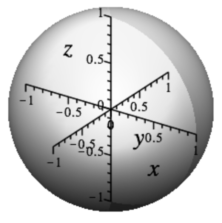
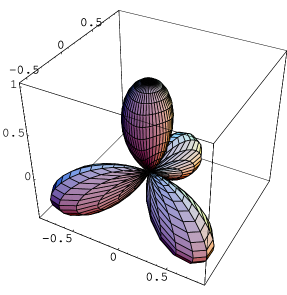
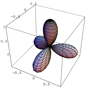
Figure 1: The potential $\Phi_{T}^{(\pm)}$ on the unit sphere. Left: $\Phi_{T}^{(+)}$ (i.e. $K=1/\sqrt{2}$); right: $\Phi_{T}^{(-)}$ (i.e. $K=-1/\sqrt{2}$). The two cases are equivalent via a rotation by an angle $(2n+1)\pi/3$. The “spherical compass” on top of these panels shows the orientation of the Cartesian frame shared by the polar plots of the octupolar potential in all remaining panels below.

All polar plots such as those in Fig. 1 are three-dimensional renderings of the surface covered by the vector $\Phi(\mathbf{e}_{r})\mathbf{e}_{r}$ as $\mathbf{e}_{r}={\mathbf{x}}/|{\mathbf{x}}|$ spans the unit sphere $S^{2}$. Since $\Phi(\mathbf{e}_{r})=-\Phi(-\mathbf{e}_{r})$, in all these plots the minima of $\Phi$ are invaginated underneath its maxima.

In angular coordinates, from (73) we have

$$\Psi_{T}^{(\pm)}=\sin^{3}\vartheta_{1}-\frac{3}{2}\sin\vartheta_{1}\cos^{2}\vartheta_{1}\mp\frac{1}{\sqrt{2}}\sin 3\vartheta_{1}\cos^{3}\vartheta_{1}.$$ (80)

See Fig. 2 for a contour plot of this function. All contour plots such as those in Fig. 2 are on the plane $(\vartheta_{2},\vartheta_{1})$, which develops the unit sphere $S^{2}$ so that the upper side $\vartheta_{1}={\pi}/{2}$ corresponds to the North Pole and the lower side $\vartheta_{1}=-{\pi}/{2}$ corresponds to the South Pole.

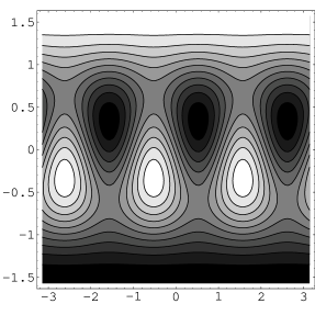
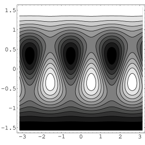
Figure 2: Contour plots of the potentials $\Psi_{T}^{(+)}$ (left) and $\Psi_{T}^{(-)}$ (right) on the plane $(\vartheta_{2},\vartheta_{1})$; see (80). In these plots, as in the others that follow, the brightest points represent the maxima of the potential, whereas the darkest points represent the minima. One easily checks that there are indeed 14 critical points (two of them at the poles). The symmetry properties of $\Psi_{T}^{(\pm)}$ are evident from this picture. The upper and lower border, at $\vartheta_{1}=\pm\pi/2$, correspond to the North and South Poles, respectively. The two plots are coincident up to a shift in $\vartheta_{2}$, in accord with the predicted invariance under $\gamma_{1}$ in (77).

The potential is obviously invariant under shifts by $(2/3)\pi$ in $\vartheta_{2}$, and that parameter inversion $K\to-K$ is equivalent to an inversion or to a shift by $\pi/3$ in $\vartheta_{2}$; i.e.

$$\Psi_{T}^{(\pm)}(\vartheta_{1},\vartheta_{2}+2\pi/3) = \Psi_{T}^{(\pm)}(\vartheta_{1},\vartheta_{2}),$$ (81)

$$\Psi_{T}^{(-)}(\vartheta_{1},\vartheta_{2}) = \Psi_{T}^{(+)}(\vartheta_{1},-\vartheta_{2})=\Psi_{T}^{(-)}(\vartheta_{1},\vartheta_{2}+\pi/3).$$ (82)

These properties imply that it suffices to study one of the two cases, say $\Psi_{T}^{(+)}$; from now on we will just consider this, and refer to it simply as $\Psi_{T}$ (and correspondingly for $\Phi^{(+)}_{T}$ and $\Phi_{T}$).

Eigenvalues and the corresponding critical points (i.e. normalized eigenvectors) for $\Phi_{T}$ are listed in Table 4 below (recall that $\lambda=\Phi$ at critical points).

Table 4: Critical points for tetrahedral symmetry; here $\nu_{m}=\arcsin(1/3)$, $\nu_{s}=\arcsin(1/\sqrt{3})$.

$n$	$\lambda$	$\vartheta_{1}$	$\vartheta_{2}$	$\Psi$	type
1	-1	$-\pi/2$	–	$-1$	min
2	-1	$-\nu_{m}$	$-\pi/2$	$-1$	min
3	-1	$-\nu_{m}$	$5\pi/6$	$-1$	min
4	-1	$-\nu_{m}$	$\pi/6$	$-1$	min
5	0	$-\nu_{s}$	$-\pi/2$	0	saddle
6	0	$-\nu_{s}$	${5\pi}/{6}$	0	saddle
7	0	$-\nu_{s}$	$\pi/6$	0	saddle
8	0	$\nu_{s}$	$\pi/2$	0	saddle
9	0	$\nu_{s}$	$-{5\pi}/{6}$	0	saddle
10	0	$\nu_{s}$	$-\pi/6$	0	saddle
11	1	$\nu_{m}$	$\pi/2$	1	max
12	1	$\nu_{m}$	${5\pi}/{6}$	1	max
13	1	$\nu_{m}$	$-\pi/6$	1	max
14	1	$\pi/2$	–	1	max

7.3 Symmetry $D_{\infty h}$: center $\mathcal{C}$

At the center $\mathcal{C}$ of the cylinder $\mathsf{C}$, i.e. for $K=\rho=0$, the potential in (74) is just

$$\Phi_{\infty}=z^{3}-\ \frac{3}{2}(x^{2}+y^{2})z;$$ (83)

correspondingly, its variant in spherical coordinates (73) is

$$\Psi_{\infty}=\frac{1}{8}(3\sin\vartheta_{1}-5\sin 3\vartheta_{1}).$$ (84)

The symmetry under rotations (about the $z$ axis) is immediately apparent, as well as the symmetry under reflection in any vertical plane. We thus have a $D_{\infty h}$ symmetry. The potential is also covariant under inversion in $z$,

$$\Phi_{\infty}(x,y,-z)=-\Phi_{\infty}(x,y,z).$$ (85)

The critical point equations (47) are now

$$-3xz = \lambda x$$

$$-3yz = \lambda y$$ (86)

$$3z^{2}-\frac{3}{2}(x^{2}+y^{2}) = \lambda z,$$

It follows immediately from the first two equations that the critical points not lying at the poles of the sphere have $\lambda=-3z$. More precisely, inserting this into the third equation – and recalling that $x^{2}+y^{2}=1-z^{2}$ – it turns out that for these we have

$$z=\pm 1/\sqrt{5},\quad\lambda=\mp 3/\sqrt{5}.$$ (87)

All points on this circle are (obviously, degenerate) critical ones; the only non-degenerate critical points are the maximum and the minimum in the North and South Poles.

We get of course the same result working in angular coordinates. From (84), we have that the critical points are located in the North and South Poles ($\vartheta_{1}=\pm\pi/2$, value $\pm 1$); and on the parallels with $\vartheta_{1}=\pm\arccos(2/\sqrt{5})\doteq\pm 0.46$. In particular, we have a circle of degenerate minima (value $-1/\sqrt{5}$) for $\vartheta_{1}=\arccos(2/\sqrt{5})$, and a circle of degenerate maxima (value $1/\sqrt{5}$) for $\vartheta_{1}=-\arccos(2/\sqrt{5})$.

The critical points are all non-degenerate modulo the degeneration enforced by the SO(2) symmetry (this also requires one of the eigenvalues of the Hessian to be zero). Critical points at the poles have an Hessian with nontrivial eigenvalue $\sigma_{0}=\pm 6$; those on the circles have an Hessian with nontrivial eigenvalue $\sigma_{1}=\pm 12/\sqrt{5}$. This case is depicted in Fig.3.

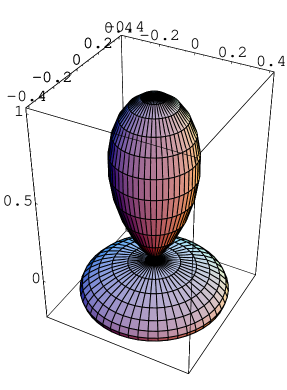
(a)	(b)

Figure 3: The potential $\Psi_{\infty}$ depends only on $\vartheta_{1}$. $(a)$ Plot of $\Psi_{\infty}$ as a function of $\vartheta_{1}$: we observe the (circle of) maxima for $\vartheta_{1}=\arcsin{(-1/\sqrt{5})}\doteq-0.46$, and the (circle of) minima for $\vartheta_{1}=\arcsin(1/\sqrt{5})$. $(b)$ The potential $\Phi_{\infty}$ as a “spherical plot”: again we observe the circle of maxima at $z=-1/\sqrt{5}$, and the circle of minima for $z=1/\sqrt{5}$.

7.4 Simmetry $D_{3h}$: the axis $\mathcal{A}$

On the axis $\mathcal{A}$ of the cylinder (i.e. for $\rho=0$), the potential in (74) reads

$$\Phi_{3}=Ky(y^{2}-3x^{2})+z\left(z^{2}-\frac{3}{2}(x^{2}+y^{2})\right),$$ (88)

and the potential expressed in (73) in angular coordinates is

$$\Psi_{3}=\sin^{3}\vartheta_{1}-K\cos^{3}\vartheta_{1}\sin 3\vartheta_{2}-\frac{3}{2}\cos^{2}\vartheta_{1}\sin\vartheta_{1}.$$ (89)

Of course, we need only consider points different from the special points $\mathcal{C}$ and $\mathcal{T}$ considered before. Here $K\geq 0$ is a free parameter. Graphical illustrations of both $\Phi_{3}$ and $\Psi_{3}$ are shown in Figs. 4 and 5.

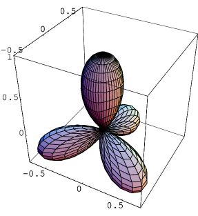
$K=1/4$	$K=1/2$
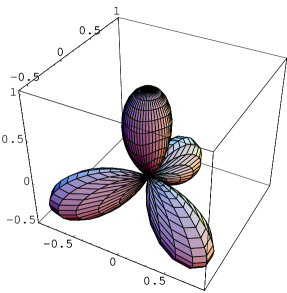
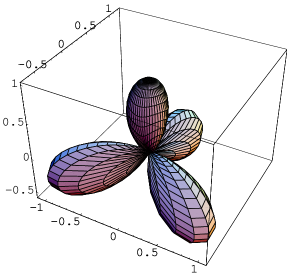
$K=3/4$	$K=1$

Figure 4: Polar plots of the potential $\Phi_{3}$ for different values of the parameter $K$. For low $K$ the maximum in the North Pole is the highest, while for higher $K$ it becomes smaller than the three symmetric maxima in the southern hemisphere.

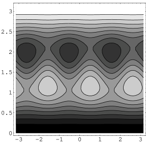
$K=1/4$	$K=1/2$
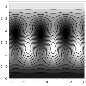
$K=3/4$	$K=1$

Figure 5: The same as in Fig. 4 but with contour plots. Note again that for low $K$ the maximum in the North Pole is the highest, while for higher $K$ it becomes smaller than the three symmetric maxima in the southern hemisphere.

The potential is invariant under the inversion $x\to-x$ and under rotations by $2\pi/3$ around the $z$ axis (i.e. shift by $2\pi/3$ in $\vartheta_{2}$; thus it would suffice to study the potential in the sector $0\leq\vartheta_{2}\leq 2\pi/3$; that is, its symmetry group is fully described by the matrices

$$\left(\begin{array}[]{lll}1&0&0\\ 0&1&0\\ 0&0&1\end{array}\right),\ \left(\begin{array}[]{lll}-\frac{1}{2}&-\frac{\sqrt{3}}{2}&0\\ \frac{\sqrt{3}}{2}&-\frac{1}{2}&0\\ 0&0&1\end{array}\right),\ \left(\begin{array}[]{lll}-\frac{1}{2}&\frac{\sqrt{3}}{2}&0\\ -\frac{\sqrt{3}}{2}&-\frac{1}{2}&0\\ 0&0&1\end{array}\right);$$ (99)

(100)

$$\left(\begin{array}[]{lll}-1&0&0\\ 0&1&0\\ 0&0&1\end{array}\right),\ \left(\begin{array}[]{lll}\frac{1}{2}&-\frac{\sqrt{3}}{2}&0\\ -\frac{\sqrt{3}}{2}&-\frac{1}{2}&0\\ 0&0&1\end{array}\right),\ \left(\begin{array}[]{lll}\frac{1}{2}&\frac{\sqrt{3}}{2}&0\\ \frac{\sqrt{3}}{2}&-\frac{1}{2}&0\\ 0&0&1\end{array}\right).$$ (110)

The potential is of course also covariant under inversion,

$$\Phi_{3}(-\vartheta_{1},-\vartheta_{2})=-\Phi_{3}(\vartheta_{1},\vartheta_{2}),$$ (111)

which corresponds to $(x,y,z)\to(-x,-y,-z)$; thus it suffices to consider $\vartheta_{1}>0$ (i.e. the northern hemisphere, as we already know from general discussion).

The critical point equations are now

$$\cos\vartheta_{1}(\cos^{2}\vartheta_{1}-4\sin^{2}\vartheta_{1}-K\sin 2\vartheta_{1}\sin 3\vartheta_{2}) = 0,$$

$$K\cos^{3}\vartheta_{1}\cos 3\vartheta_{2} = 0.$$

The second of these implies that critical points are either at the poles, with $\vartheta_{1}=\pm\pi/2$ (there is of course a maximum, value $\Phi_{3}=1$, at the North Pole; and a minimum, value $\Phi_{3}=-1$, at the South Pole), or on the meridians identified by

$$\vartheta_{2}\ =\pm\frac{\pi}{6},\pm\frac{\pi}{2},\pm\frac{5\pi}{6}.$$ (113)

As $\vartheta_{2}$ enters the equations only through terms $3\vartheta_{2}$, it is obvious that cases with $\vartheta_{2}$ differing by $2\pi/3$ are equivalent (so the cases $\vartheta_{2}=-\pi/2,+\pi/6,+5\pi/6$ are equivalent to each other, and so are the cases $\vartheta_{2}=-5\pi/6,-\pi/6,\pi/2$); it thus suffices to consider $\vartheta_{2}=\pm{\pi}/{6}$ , which yields $\sin 3\vartheta_{2}=\pm 1$. With this choice for $\vartheta_{2}$, the first of (LABEL:eq:d3hcrit) reads

$$\cos\vartheta_{1}\left(3-5\cos 2\vartheta_{1}\pm\ 2K\sin 2\vartheta_{1}\right)=0.$$ (114)

Assuming $\vartheta_{1}\not=\pm\pi/2$, this further reduces to

$$\cos^{2}\vartheta_{1}-4\sin^{2}\vartheta_{1}\mp\ 2K\sin\vartheta_{1}\cos\vartheta_{1}=0.$$ (115)

Writing $\eta=\tan\vartheta_{1}$, and taking off an overall factor $\cos^{2}\vartheta_{1}\not=0$, this reads

$$1-4\eta^{2}\mp 2K\eta=0.$$ (116)

Thus for $\vartheta_{2}=-5\pi/6,-\pi/6,\pi/2$ we get

$$\eta^{-}_{\pm}=-\frac{K}{4}\left(1\pm\sqrt{1+4/K^{2}}\right),$$ (117)

while for $\vartheta_{2}=-\pi/2,\pi/6,5\pi/6$ we get

$$\eta^{+}_{\pm}=\frac{K}{4}\left(1\pm\sqrt{1+4/K^{2}}\right).$$ (118)

This means that we have in total twelve nontrivial critical points, i.e. fourteen counting also those at the poles. We know (see Sect. 5.4) that four of these will be maxima, other four will be minima, and the remaining six will be saddles.

Recalling that $-\pi/2<\vartheta_{1}<\pi/2$, one then easily shows that critical points can be represented as $\vartheta_{1}=\xi^{\pm}_{\pm}$, where

$$\xi^{+}_{\pm}=\arcsin\left(\eta^{+}_{\pm}/\sqrt{1+(\eta^{+}_{\pm})^{2}}\right),\quad\xi^{-}_{\pm}=\arcsin\left(\eta^{-}_{\pm}/\sqrt{1+(\eta^{-}_{\pm})^{2}}\right).$$ (119)

To characterize the nature of critical points, we can either consider the potential on the meridians (113) and on the parallels identified by (119) (with the aid of (117) and (118)); or study the eigenvalues of the Hessian at these critical points. In fact, the eigenvalues of the Hessian on $\vartheta_{2}=\pi/6$ (and equivalent meridians) are

$$\Lambda^{+}=\left\{9K\cos^{3}\vartheta_{1},\frac{3}{8}\left(2K\cos\vartheta_{1}+6K\cos 3\vartheta_{1}-\sin\vartheta_{1}+15\sin 3\vartheta_{1}\right)\right\},$$ (120)

while those on $\vartheta_{2}=-\pi/6$ (and equivalent meridians) are

$$\Lambda^{-}=\left\{-9K\cos^{3}\vartheta_{1},-\frac{3}{8}\left(2K\cos\vartheta_{1}+6K\cos 3\vartheta_{1}+\sin\vartheta_{1}-15\sin 3\vartheta_{1}\right)\right\}.$$ (121)

Recalling that $\cos\vartheta_{1}>0$ and $K>0$, which fixes the sign of the first eigenvalue in both cases, we see that on $\vartheta_{2}=\pi/6$ (and equivalent meridians) we can only have saddles or minima, and on $\vartheta_{2}=-\pi/6$ (and equivalent meridians) we can only have maxima or saddles.

The above formulas (120), (121) also allow us to compute explicitly the eigenvalues at critical points, and hence the nature of these. The results are summarized in Table 5 (which also includes the critical points at the poles, considered as trivial in the previous discussion); we stress that there is no change of stability as $K$ is varied, as follows from (120), (121).

To improve readability of Table 5, we have used the shorthand notations

$$q_{\pm} := \left[10+K^{2}\pm K\sqrt{4+K^{2}}\right]^{-1},$$

$$\tau_{\pm} := \arcsin\left(\frac{\kappa_{\pm}q_{\pm}}{2}\right),$$ (122)

$$\zeta_{\pm} := \sqrt{2q_{\pm}^{3}}\left[K^{3}\pm K^{2}\sqrt{4+K^{2}}+13K\mp 5\sqrt{4+K^{2}}\right].$$

Table 5: Critical points for the case $D_{3h}$. The relation prescribed by eq.(53) are satisfied, hence $\lambda$ is not displayed. The shorthand notation (122) is used.

$n$	$\vartheta_{1}$	$\vartheta_{2}$	$\Psi$	type
1	$-\pi/2$	$--$	-1	min
2	$-\tau_{-}$	$-\pi/2$	$-\zeta_{-}$	min
3	$-\tau_{-}$	$\pi/6$	$-\zeta_{-}$	min
4	$-\tau_{-}$	$5\pi/6$	$-\zeta_{-}$	min
5	$-\tau_{+}$	$-\pi/2$	$-\zeta_{+}$	saddle
6	$-\tau_{+}$	$\pi/6$	$-\zeta_{+}$	saddle
7	$-\tau_{+}$	$5\pi/6$	$-\zeta_{+}$	saddle
8	$\tau_{+}$	$-5\pi/6$	$\zeta_{+}$	saddle
9	$\tau_{+}$	$-\pi/6$	$\zeta_{+}$	saddle
10	$\tau_{+}$	$\pi/2$	$\zeta_{+}$	saddle
11	$\tau_{-}$	$-5\pi/6$	$\zeta_{-}$	max
12	$\tau_{-}$	$-\pi/6$	$\zeta_{-}$	max
13	$\tau_{-}$	$\pi/2$	$\zeta_{-}$	max
14	$\pi/2$	$--$	1	max

Remark 17.

We note that the value of the potential at the non-orienting maxima – i.e. at the critical points 11, 12, and 13 in Table 5, is in explicit terms

$$\zeta_{-}=\frac{\sqrt{2}\left(K^{3}-\sqrt{K^{2}+4}K^{2}+13K+5\sqrt{K^{2}+4}\right)}{\left(K^{2}-\sqrt{K^{2}+4}K+10\right)^{3/2}};$$ (123)

it is a simple matter to check this is always (positive and) increasing with $K$, and that $\zeta_{-}=1$ for $K=K_{0}:=\sqrt{2}/2\doteq 0.71$. Thus, these are secondary maxima for $K<K_{0}$, and become absolute maxima for $K>K_{0}$. We thus have a “global bifurcation” between the phases $D_{3h}^{+}$ and $D_{3h}^{-}$ taking place at $K=K_{0}$. For this value of $K$, the value taken by the potential at the saddle points 5–10 in Table 5 is $\zeta_{+}=0$. It should also be noted that $\zeta_{+}$ is always increasing with $K$. $\odot$

Remark 18.

Let us focus on the maxima. In those other than the North Pole, we have $\Phi=\Phi_{M}$ and $\lambda=\lambda_{M}$. These are smaller than the corresponding quantities for the maximum in the North Pole for $K<K_{0}$, and greater than those for $K>K_{0}$. In other words, albeit at $K=K_{0}$ there is no local bifurcation, we have a rearrangement of the maxima and saddles in terms of their ordering according to value of the potential. When choosing the orienting maximum, we could also choose it in such a way that it should always be the largest; this means that the case with $K>K_{0}$ necessarily corresponds to a case present with other values of the parameters, in which the orienting maximum is the largest. Such a choice would break the $D_{3h}$ symmetry around the orienting axis, and we would be left with a $D_{2h}$ symmetry around the new orienting axis. $\odot$

Remark 19.

Inverting the relation between $K$ and $\lambda$, we can express $K$ in terms of $\lambda$; similarly, we can invert the relation between $K$ and $\vartheta_{1}$. Eliminating $K$ from these two equations according to the two variants in (119), they provide the corresponding (not too simple) relations linking $\lambda_{S}$ and $\lambda_{M}$ with $\vartheta_{1}$, for saddles and maxima, respectively; more precisely, we have

$$\lambda_{S}=\frac{1}{2}\frac{2-3\cos^{2}\vartheta_{1}}{\sin\vartheta_{1}},\quad\lambda_{M}=\ \frac{8-9\cos^{2}\vartheta_{1}}{\cos\vartheta_{1}\sqrt{16-15\cos^{2}\vartheta_{1}}}.$$ (124)

$\odot$

7.4.1 Symmetry breaking: from $D_{\infty h}$ to $D_{3h}$

It is interesting to consider the situation in the $D_{3h}$ phase for values of $K$ near zero; in other words, to consider the symmetry breaking from $D_{\infty h}$ (case $K=0$, the center of the disk $\mathcal{D}$) to $D_{3h}$.

We will write $K=\varepsilon$ and work at first order in $\varepsilon$. With this, we obtain easily

$$\cos\vartheta_{1}=\frac{10+\varepsilon}{5\sqrt{5}};$$ (125)

in the same way we also get

$$\lambda_{M}=\frac{15+24\varepsilon}{5\sqrt{5}}.$$ (126)

In particular, denoting by a “0” the limit for $K\to 0$, we have

$$\frac{\lambda_{M}-\lambda_{M}^{0}}{\cos\vartheta_{1}-\cos\vartheta_{1}^{0}}=24+O(\varepsilon).$$ (127)

7.4.2 Symmetry breaking: from $T_{d}$ to $D_{3h}$

We can also consider the symmetry breaking from the tetrahedral phase to $D_{3h}$. In this case we will write $K=K_{0}+\varepsilon$ and work again at first order in $\varepsilon$. Now we get

$$\cos\vartheta_{1}=\frac{2\sqrt{2}}{3}+\frac{4}{81}\varepsilon,\quad\lambda_{M}=3+\frac{16\sqrt{2}}{9}\varepsilon.$$ (128)

Thus in this case, denoting now by a superscript ^T the tetrahedral limit, we have

$$\frac{\lambda_{M}-\lambda^{T}}{\cos\vartheta_{1}-\cos\vartheta_{1}^{T}}=\ 36\sqrt{2}+O(\varepsilon).$$ (129)

7.5 Simmetry $D_{2h}$: the disk $\mathcal{D}$

On the disk $\mathcal{D}$ identified by $K=0$ (with $\rho\not=0$, or we would be at the center $\mathcal{C}$ and in case $D_{\infty h}$ considered above), we have a symmetry $D_{2h}$. In fact, the potential in (74) reduces to

$$\Phi_{2}=z^{3}-3y^{2}z+3\rho\cos\chi xyz+\frac{3}{2}(\rho\sin\chi-1)\left(x^{2}-y^{2}\right)z,$$ (130)

and similarly its counterpart in angular coordinates is readily obtained from (73) as

$$\Psi_{2}=\sin\vartheta_{1}\left[\sin^{2}\vartheta_{1}+\frac{3}{2}\cos^{2}\vartheta_{1}(\rho\sin(\chi+2\vartheta_{2})-1)\right].$$ (131)

Graphical illustrations for both $\Phi_{2}$ and $\Psi_{2}$ in the styles introduced above are provided in Figs. 6, 7, and 8.

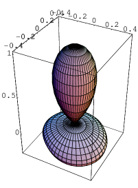
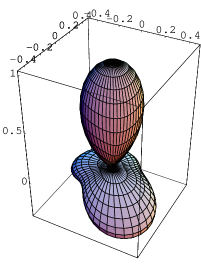
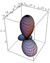
$\rho=0.1$	$\rho=0.3$	$\rho=0.5$
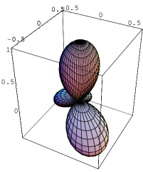
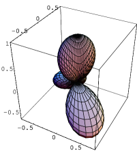
$\rho=0.7$	$\rho=0.9$	$\rho=1.1$
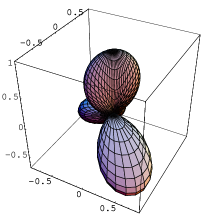
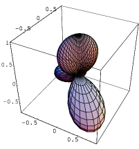
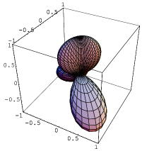
$\rho=1.3$	$\rho=1.5$	$\rho=1.7$

Figure 6: The potential $\Phi_{2}$ for $\chi=0$ and different values of the parameter $\rho$.

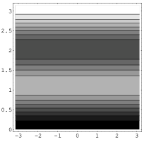
$\rho=0$	$\rho=0.1$	$\rho=0.3$
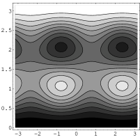
$\rho=0.5$	$\rho=0.7$	$\rho=0.9$
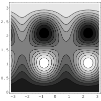
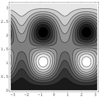
$\rho=1.1$	$\rho=1.3$	$\rho=1.5$
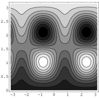
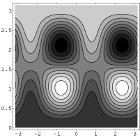
$\rho=1.7$	$\rho=1.9$	$\rho=2$

Figure 7: Contour plot of the potential $\Psi_{2}$ for $\chi=0$ and for various values of $\rho>0$. There always are three maxima, three minima and four saddles; for $\rho 1.0$, pairs of saddles originally one on top of the other collide and re-emerge side to side. See Fig. 8 for more details.

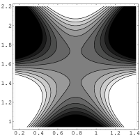
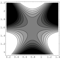
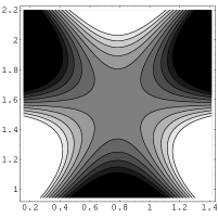
$\rho=0.95$	$\rho=0.97$	$\rho=0.99$
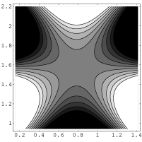
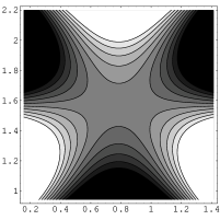
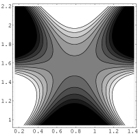
$\rho=1.01$	$\rho=1.03$	$\rho=1.05$

Figure 8: Contour plot of the potential $\Psi_{2}$ in the region where the saddle/saddle bifurcation takes place (here $\vartheta_{1}\in[-\pi/5,\pi/5]$, $\vartheta_{2}\in[\pi/4-\pi/5,\pi/4+\pi/5]$) for $\chi=0$ and for various values of $\rho$. We observe the saddle/saddle bifurcation taking place; in this a pairs of saddles originally one on top of the other collide (at $\rho=1.0$) and re-emerge side to side. At $\rho=1.0$ there is a monkey saddle.

Remark 20.

It is clear from this expression that a shift in $\chi$ corresponds to a shift (of half the amplitude) in $\vartheta_{2}$; see also Fig. 9 for a visual demonstration. $\odot$

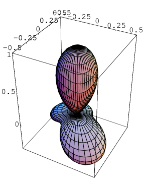
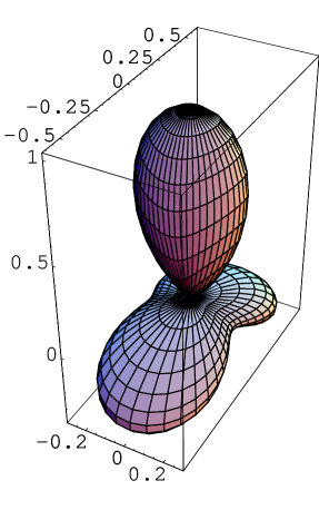
Figure 9: Three-dimensional polar plot of the potential $\Phi_{2}$, see (131), for $\rho=0.4$. Here we have chosen $\chi=0$ (left) and $\chi=\pi/2$ (right). It is clear that the rotations by $\pi/2$ in $\chi$ corresponds to a rotation by $\pi/4$ in $\vartheta_{2}$.

Remark 21.

It is also apparent from (131) that $\Psi_{2}$ is identically zero on the Equator $\vartheta_{1}=0$ (i.e. $\Phi_{2}$ is identically zero for $z=0$); this implies that any critical point lying on the Equator will necessarily be non-hyperbolic, hence degenerate. $\odot$

Remark 22.

The invariance under rotations by $\pi$ in $\vartheta_{2}$ is evident. We also have invariance under rotations by any $\delta$ in $\vartheta_{2}$ accompanied by a rotation by $2(\pi-\delta)$ in $\chi$. In particular, we have invariance under a rotation by $\pi/2$ in $\vartheta_{2}$ accompanied by a rotation by $\pi$ in $\chi$; thus, we can just consider $-\pi/2\leq\chi\leq\pi/2$.

We could also restrict the domain in which we study the potential by noting that $\Psi_{2}\to-\Psi_{2}$ under $\vartheta_{1}\to-\vartheta_{1}$; this also follows by the usual skew-symmetry of the potential under the antipodal map combined with invariance under $\vartheta_{2}\to\vartheta_{2}+\pi$. $\odot$

7.5.1 Symmetry of the potential

The potential is invariant under a subgroup $O(2)\subset T_{d}$; this is explicitly given by the matrices

$$M_{0}\ =\left(\begin{array}[]{lll}1&0&0\\ 0&1&0\\ 0&0&1\end{array}\right),\quad M_{\pi}=\left(\begin{array}[]{lll}-1&0&0\\ 0&-1&0\\ 0&0&1\end{array}\right);$$ (132)

$$R_{1}=\left(\begin{array}[]{ccc}-\sin\chi&-\cos\chi&0\\ -\cos\chi&\sin\chi&0\\ 0&0&1\end{array}\right),\ R_{2}=\left(\begin{array}[]{ccc}\sin\chi&\cos\chi&0\\ \cos\chi&-\sin\chi&0\\ 0&0&1\end{array}\right).$$ (133)

Both $M_{0}$ and $M_{\pi}$ have determinant $+1$, while both $R_{1}$ and $R_{2}$ have determinant $-1$.

The matrices $R_{i}$ describe a reflection in a vertical plane. More precisely, recalling that the matrix describing a reflection in the vertical plane $y=mx$ is given by

$$R_{m}=\left(\begin{array}[]{lll}a&\ b&0\\ b&-a&0\\ 0&\ 0&1\end{array}\right),\quad a=\frac{1-m^{2}}{m^{2}+1},\quad b=\frac{2m}{m^{2}+1},$$ (134)

and that conversely a matrix $R_{m}$ as in (134) with $a^{2}+b^{2}=1$ represents a reflection through the plane $y=mx$ with

$$m=\frac{1-a}{b},$$ (135)

the planes of reflection for the matrices $R_{i}$ (orthogonal to one another) have equations $y=m_{i}x$, where

$$m_{1}=-\frac{1+\sin\chi}{\cos\chi},\quad m_{2}=\frac{1-\sin\chi}{\cos\chi},$$ (136)

which clearly satisfy $m_{1}m_{2}=-1$.

We have special cases for $\chi=\pm\pi/2$ or $\chi=0,\pi$ (note that when both these conditions are met, we are back to the case $\rho=0$ considered above; in fact, we have characterized $D_{2h}$ by also requiring $\rho\not=0$).

Remark 23.

To appreciate better our previous Remark 20, consider the case $\chi=0$. Now $R_{i}$ read as

$$R_{1}=\left(\begin{array}[]{ccc}0&-1&0\\ -1&0&0\\ 0&0&1\end{array}\right),\quad R_{2}=\left(\begin{array}[]{ccc}0&1&0\\ 1&0&0\\ 0&0&1\end{array}\right).$$ (137)

These represent reflections in the vertical planes $y=x$ and $y=-x$, as illustrated in the left panel of Fig. 9. $\odot$

7.5.2 Critical points

The critical points are identified as solutions to the equations

$$\frac{3}{4}\cos\vartheta_{1}[-5\cos 2\vartheta_{1}+\rho(3\cos 2\vartheta_{1}-1)\sin(\chi+2\vartheta_{2})+3] = 0,$$

$$3\rho\cos^{2}\vartheta_{1}\cos(\chi+2\vartheta_{2})\sin\vartheta_{1} = 0.$$

Remark 24.

It is immediately apparent that any change in $\chi$ can be compensated by a change in $\vartheta_{2}$, and conversely; in other words, the relevant angle is $\Theta=(\vartheta_{2}+\chi/2)$. Thus it suffices to study the problem with a given value of $\chi$, e.g., $\chi=\pi/2$ (hence $\alpha_{0}=\rho$, $\gamma=0$) or $\chi=0$ (hence $\alpha_{0}=0$, $\gamma=\rho$); the general case (i.e. the case of general $\chi$) will be obtained via a suitable rotation in $\vartheta_{2}$.

Solving equations (LABEL:eq:ecpd2h) in general is a matter of standard algebra and trigonometry (and some patience). The results are reported in Table 6 below; it should be stressed that some of the solutions exist only for certain ranges of $\rho$.

Let us first focus on the second of (LABEL:eq:ecpd2h); discarding as usual the ”trivial” (in this context) solutions for $\vartheta_{1}=\pm\pi/2$, which corresponds to the poles, we need either $\cos(\chi+2\vartheta_{2})=\pm\pi/2$; or $\vartheta_{1}=0$. But inserting $\vartheta_{1}=0$ in the first of (LABEL:eq:ecpd2h), we obtain

$$-\frac{3}{2}\left[1-\rho\sin(\chi+2\vartheta_{2})\right]=0.$$ (139)

This admits solutions only for $\rho\geq 1$; in view of our general restriction on $\rho$, see (72), this means $\rho\in[1,2]$.

On the other hand, if $\cos(\chi+2\vartheta_{2})=0$, i.e. $\chi+2\vartheta_{2}=\pm\pi/2$, and hence $\sin(\chi+2\vartheta_{2})=\pm 1$, the first of (LABEL:eq:ecpd2h) reads (after taking away the inessential factor $(3/4)\cos\vartheta_{1}$)

$$3-5\cos 2\vartheta_{1}\mp\rho(1-3\cos 2\vartheta_{1})=0;$$ (140)

this means

$$\cos 2\vartheta_{1}=\frac{3\mp\rho}{5\mp 3\rho}.$$ (141)

While the solution with the plus sign does exist for all values of $\rho$, the solution with the minus sign exists only for $\rho=2$ and $\rho\leq 1$.

In other words, we have some family of solutions existing through the whole range $\rho\in[0,2]$, while for other families we will have to consider separately the subranges $\rho\in[0,1]$ and $\rho\in[1,2]$. It has to be expected (and it will indeed result) that a multiple bifurcation takes place at $\rho=1$. It should be noted that at the bifurcation point the saddles are degenerate, so carrying a different index.

The situation is rather clear if we think of a fixed value of $\chi$, say $\chi=\pi/2$, and focus only on families of solutions not existing for the whole range of $\rho$ (it turns out that all of these are saddles). For $\rho\in[0,1)$ there are solutions on the meridians identified by $\chi+2\vartheta_{2}=(k+1/2)\pi$ and approaching the Equator as $\rho\to 1$, but none on the equator; on the other hand, for $\rho\in(1,2]$ there are no solutions on those meridians, but we have instead families of solutions on the Equator, drifting away from the meridians identified by $\chi+2\vartheta_{2}=(k+1/2)\pi$ as $\rho$ grows away from $\rho=1$. This is clearly illustrated in Fig.10.

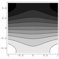
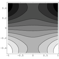
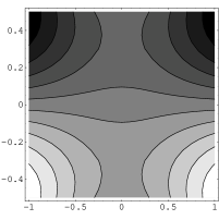
$\rho=0.2$	$\rho=0.4$	$\rho=0.6$
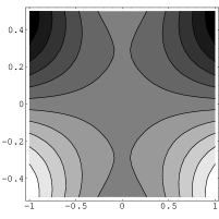
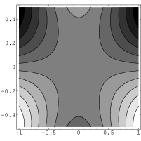
$\rho=0.8$	$\rho=1.0$	$\rho=1.2$
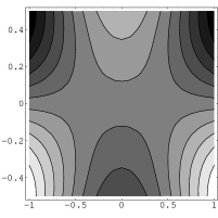
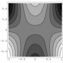
$\rho=1.4$	$\rho=1.6$	$\rho=1.8$

Figure 10: The saddle-saddle bifurcation in the $D_{2h}$ case taking place at $\rho=1$. We have chosen $\chi=\pi/2$ and plotted a neighborhood of the point $(\vartheta_{1},\vartheta_{2})=(0,0)$ – more precisely the region $|\vartheta_{1}|\leq 1/2$, $|\vartheta_{2}|\leq 1$ – as $\rho$ is varied. The two saddles located (symmetrically w.r.t. the Equator) on the meridian $\vartheta_{2}=0$ collide at $\rho=1$, giving raise to a new pair of saddles located on the Equator, symmetrically w.r.t. the meridian $\vartheta_{2}=0$.

We now return to the solutions to the critical point equations (LABEL:eq:ecpd2h). The nature of these critical points is easily ascertained by considering the eigenvalues of the Hessian at them; again the result of this analysis is reported in Table 6. Here again we resort to some shorthand notation to make the table more readable; in that we have defined

$$\rho_{\pm} := \frac{\rho\pm 3}{3\rho\pm 5},\quad r_{\pm}:=\arccos\left(\rho_{\pm}\right),\quad r_{0}:=\arccos\left(1/\rho\right),$$

$$\mu_{\pm} := \frac{\chi}{2}\pm\frac{\pi}{4},\quad\nu_{\pm}:=\frac{\chi}{2}\pm\frac{3\pi}{4},\qquad\ \omega_{\pm}:=\frac{\chi\pm r_{0}}{2}.$$

Table 6: Critical points for the case $D_{2h}$. The shorthand notation (LABEL:eq:d2hshortnot) is used here.

$n$	$\vartheta_{1}$	$\vartheta_{2}$	$\Psi$	range	type
1	$-{\pi}/{2}$	—	$-1$	always	min
2	$r_{+}$	$-\mu_{+}$	$-(\rho+1)\sin r_{+}$	always	min
3	$r_{+}$	$-\nu_{-}$	$-(\rho+1)\sin r_{+}$	always	min
4	$r_{-}$	$-\mu_{-}$	$(\rho-1)\sin r_{-}$	$\rho\leq 1$	saddle
5	$-r_{-}$	$-\mu_{-}$	$-(\rho-1)\sin r_{-}$	$\rho\leq 1$	saddle
6	$-r_{-}$	$-\nu_{+}$	$-(\rho-1)\sin r_{-}$	$\rho\leq 1$	saddle
7	$r_{-}$	$-\nu_{+}$	$(\rho-1)\sin r_{-}$	$\rho\leq 1$	saddle
8	0	$-\omega_{-}$	0	$\rho\geq 1$	saddle
9	0	${\pi}/{2}-\omega_{+}$	0	$\rho\geq 1$	saddle
10	0	$\pi-\omega_{-}$	0	$\rho\geq 1$	saddle
11	0	$-\omega_{+}-{\pi}/{2}$	0	$\rho\geq 1$	saddle
12	$-r_{+}$	$-\mu_{+}$	$(\rho+1)\par\sin r_{+}$	always	max
13	$-r_{+}$	$-\nu_{-}$	$(\rho+1)\sin r_{+}$	always	max
14	${\pi}/{2}$	—	1	always	max

Remark 25.

Looking at Table 6, we note that maxima and minima belong to families running through the whole range of admitted values for $\rho$, while the saddles undergo bifurcations. For $\rho\leq 1$ the four saddles are at symmetric points on two opposite meridians (for $\chi=\pi/2$ these are identified by $y=0$) and drift towards the Equator as $\rho$ approaches the critical value $\rho=1$, while for $\rho>1$ the four saddles are at symmetric points on the equator and drift away from the previously mentioned meridians as $\rho$ increases. This means that there is a (saddle/saddle) local bifurcation. $\odot$

Remark 26.

Note also that a global change takes place at the same value $\rho=1$. That is, for $\rho<1$ the orienting local maximum in the North Pole is also the absolute maximum, the other two being (degenerate and) lower than this; for $\rho>1$, on the other hand, the other two maxima are (degenerate and) higher than the orienting one. Similarly to what we have done for the $D_{3h}$ phase, we will distinguish these as $D_{2h}^{+}$ and $D_{2h}^{-}$ phases. $\odot$

Remark 27.

We could have defined the orientation requiring that the North Pole is not only a local maximum, but actually the absolute maximum. In this case the parameter range would be further restricted from the cylinder $\mathsf{C}$ to a subset $\mathsf{C}_{0}$; and Remark 26 shows that the intersection of $\mathsf{C}_{0}$ with the disk $\mathcal{D}$ (of radius $\rho=2$) would just be the disk of radius $\rho=1$. This would however introduce rather complex mappings involving both the physical and the parameter space GV2016 ; CQV , and we prefer not to discuss it here; the reader is referred to CQV for a detailed discussion. $\odot$

Remark 28.

If we look at the potential for $\rho=1$, say for the “reference case” $\chi=\pi/2$, it turns out this is invariant under a subgroup of the group $O(2)$ acting in the $(y,z)$ plane; this is generated by the matrices

$$M_{1} = \left(\begin{array}[]{ll}1&0\\ 0&1\end{array}\right),\ M_{2}=\left(\begin{array}[]{ll}-\frac{1}{2}&-\frac{\sqrt{3}}{2}\\ \frac{\sqrt{3}}{2}&-\frac{1}{2}\end{array}\right),\ M_{3}=\left(\begin{array}[]{ll}-\frac{1}{2}&\frac{\sqrt{3}}{2}\\ -\frac{\sqrt{3}}{2}&-\frac{1}{2}\end{array}\right);$$ (149)

$$M_{4} = \left(\begin{array}[]{ll}-1&0\\ 0&1\end{array}\right),\ M_{5}=\left(\begin{array}[]{ll}\frac{1}{2}&\frac{\sqrt{3}}{2}\\ \frac{\sqrt{3}}{2}&-\frac{1}{2}\end{array}\right),\ M_{6}=\left(\begin{array}[]{ll}\frac{1}{2}&-\frac{\sqrt{3}}{2}\\ -\frac{\sqrt{3}}{2}&-\frac{1}{2}\end{array}\right).$$ (157)

These satisfy

$$M_{2}^{3}=M_{3}^{3}=M_{4}^{2}=M_{1}=I;$$

$$M_{2}^{2}=M_{3},\quad M_{5}=M_{4}M_{2},\quad M_{6}=M_{4}M_{3};$$ (158)

$$M_{5}^{2}=M_{6}^{2}=I.$$

The $SO(2)$ matrices $\{M_{1},M_{2},M_{3}\}$ span the group $S_{3}$ of rotations through multiples of $2\pi/3$, while $\{M_{4},M_{5},M_{6}\}$ (having determinant $-1$) are reflections in $y$ – that is, in three-dimensional terms, through the plane $(x,z)$ – and through planes obtained from this by rotations of $2\pi/3$ about the $x$ axis. Thus the six matrices provide a representation of the group $D_{3}$. The potential is also obviously invariant under reflections in $x$, i.e. through the $(y,z)$ plane, hence at the bifurcation point we have a $D_{3h}$ symmetry (as on the axis $\mathcal{A}$). $\odot$

Remark 29.

Note also that the group $S_{3}$ acts mapping maxima to maxima and minima to minima; the reflections map maxima into minima and minima into maxima. Saddle points are obviously invariant, as the transformations we are considering do not act on the $x$ coordinate. $\odot$

Remark 30.

Our discussion in the last two Remarks has been conducted in the “reference case” $\chi=\pi/2$. For different values of $\chi$, we have the same situation but with an overall rotation of the whole picture (see Remark 20). $\odot$

7.5.3 Bifurcations

We are again interested in relations between the eigenvalues and the direction of eigenvectors, in particular near the bifurcation points. In this case, $\Phi_{+}=(1+\rho)\sin\xi_{+}$, where $\Phi_{+}$ is the height of the “secondary” maxima (which for $\rho>1$ are actually higher than the orienting one) and $(\xi_{+}+\pi/2)$ is the angle between these maxima and the orienting one (“secondary maxima” can be recognized by the fact they are always degenerate). We express $\rho$ in terms of $\xi_{+}$ through the equation

$$\rho=-\frac{3-5\cos 2\xi_{+}}{1-3\cos 2\xi_{+}}.$$ (159)

At the bifurcation point $\rho=1$, we have $\xi_{+}=\pi/6$ and $\Phi_{+}=1$. Thus, using (159) and with some trivial algebra, we see that

$$\Phi_{+}=4\frac{\sin^{3}\xi+}{3\cos 2\xi_{+}-1}.$$ (160)

By series expansion at the bifurcation point, i.e. for $\xi_{+}=\pi/6+\varepsilon$, we get

$$\Phi_{+}(\varepsilon)-\Phi_{+}(0)=9\sqrt{3}\varepsilon+O(\varepsilon^{2}).$$ (161)

Let us also consider the bifurcation from the $D_{\infty h}$ to the $D_{2h}$ phase, taking place at $\rho=0$. Using again (159), and writing $\xi_{+}=\xi_{+}^{(0)}+\varepsilon$ where

$$\xi_{+}^{(0)}=\frac{1}{2}\arccos\left(\frac{3}{5}\right)\doteq 0.46$$ (162)

is the value taken by $\xi_{+}$ for $\rho=0$, we get

$$\Phi_{+}(\varepsilon)-\Phi_{+}(0)=(15\cos\xi_{+}^{(0)}\sin^{2}\xi_{+}^{(0)}+30\sin^{3}\xi_{+}^{(0)})\varepsilon+O(\varepsilon^{2})\doteq 5.37\,\varepsilon+O(\varepsilon^{2}).$$ (163)

7.6 Reflection symmetry: special planes in the Bulk $\mathcal{B}$

As suggested by the classification of $T_{d}$ subgroups, see Appendix A, we expect that there are specific values of the parameters such that the potential is invariant under a reflection in a vertical plane, i.e. under a $Z_{2}=D_{h}$ group.

This is indeed the case for $\chi=\pm\pi/2$, $\chi=\pm\pi/6$, $\chi=\pm 5\pi/6$. Let us just consider the first case (the others are just obtained from this by a $2\pi/3$ rotation, see below).

For $\chi=\pm\pi/2$, the potential (74) reduces to

$$\Phi_{or}=z^{3}+Ky(y^{2}-3x^{2})-\frac{3}{2}(x^{2}+y^{2})z\pm\frac{3}{2}\rho(x^{2}-y^{2})z;$$ (164)

this is manifestly invariant under the reflection in the $(y,z)$ plane, i.e. under $x\to-x$. Equivalently, we have invariance under the subgroup of $T_{d}$ generated by $M_{13}$ (see Appendix A for the matrices $M_{i}$).

Similar considerations apply for the subgroups generated by $M_{14}$, with invariance subject to the condition $\chi=-\pi/6$ or $\chi=5\pi/6$; in this case the reflection is through the plane $x=-\sqrt{3}y$. In comolete analogy with this is the subgroup generated by $M_{15}$, where now one has to require $\chi=-5\pi/6$ or $\chi=\pi/6$; the reflection plane is then $x=\sqrt{3}y$.

We will refer to these planes (collectively) as $\mathcal{P}$; when we want to be more specific (see Table 7 at the end of this section) we will call them, respectively, $\mathcal{P}_{0}$, $\mathcal{P}_{-}$, $\mathcal{P}_{+}$. These reflection symmetries had evaded our previous studies GV2016 ; CQV and have proved quite significant in the present one.

For the special $D_{h}$ phases considered here, as for all others, the transition from the octupolar potential having four maxima to that having only three takes place for parameters chosen on the separatrix identified in our previous work GV2016 ; CQV and also recalled in the following Sect. 7.7. This is illustrated in Figs. 11 and 12. The separatrix is a surface in parameter space that marks the border between the subregions $\mathcal{B}_{3}$ and $\mathcal{B}_{4}$ of $\mathcal{B}$, where $\Phi_{or}$ has three or four maxima, respectively.

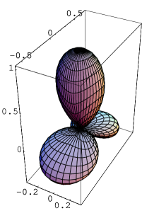
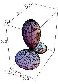
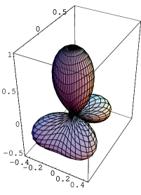
$K=0.1$	$K=0.2$	$K=0.3$
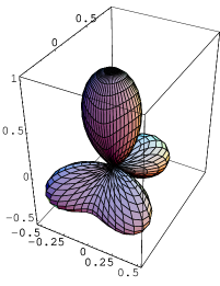
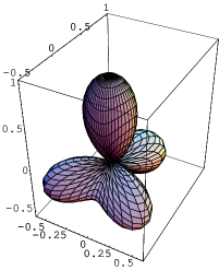
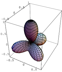
$K=0.4$	$K=0.5$	$K=0.6$

Figure 11: The potential for $\chi=\pi/2$ and $\rho=1/2$, for different values of $K>0$. We observe the transition from a phase with three maxima at low $K$ to a phase with four maxima at higher $K$. The octupolar potential is always reflection invariant through a vertical plane spanned by the axes $y$ and $z$.

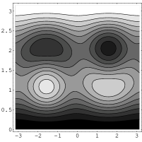
$K=0.1$	$K=0.2$	$K=0.3$
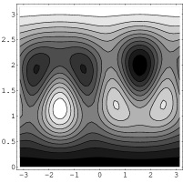
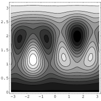
$K=0.4$	$K=0.5$	$K=0.6$

Figure 12: Same as Fig. 11 but with contour plots.

To discuss in more detail the critical points in these phases, we find it more convenient to expressing the octupolar potential in angular coordinates ans in (73).

Remark 31.

Since, by $\gamma_{3}$ in (77), the potential in (73) is invariant under the simultaneous shifts

$$\chi\,\to\,\chi\,+\,\frac{2m}{3}\pi,\ \ \vartheta_{2}\,\to\,\vartheta\,+\,\frac{2m}{3}\pi,$$

by studying the case $\chi=\pi/2$ we also obtain information about the cases $\chi=-5\pi/6$ and $\chi=-\pi/6$; and by studying the case $\chi=-\pi/2$ we also obtain information about the cases $\chi=\pi/6$ and $\chi=5\pi/6$.

We will only consider the cases $\chi=\pm\pi/2$.

7.6.1 The case $\chi=\pi/2$

By setting $\chi=\pi/2$, the potential (73) reduces to

$$\Psi_{or}=\sin^{3}\vartheta_{1}-K\cos^{3}\vartheta_{1}\sin 3\vartheta_{2}-\frac{3}{2}\sin\vartheta_{1}\cos^{2}\vartheta_{1}(1-\rho\cos 2\vartheta_{2}).$$ (165)

The conditions for a critical point are then

$$\frac{\partial\Psi_{or}}{\partial\vartheta_{1}}=0,\quad\frac{\partial\Psi_{or}}{\partial\vartheta_{2}}=0;$$ (166)

both equations have a power of $\cos\vartheta_{1}$ as an overall factor, which of course vanishes only at the poles; quotienting this factor (and constants) out, we remain with

$$K\sin 2\vartheta_{1}\sin 3\vartheta_{2}-\cos^{2}\vartheta_{1}(1-\rho\cos 2\vartheta_{2})+2\sin^{2}\vartheta_{1}(2-\rho\cos 2\vartheta_{2}) = 0,$$

$$K\cos\vartheta_{1}\cos 3\vartheta_{2}+\rho\sin\vartheta_{1}\sin 2\vartheta_{2} = 0.$$

The second equation (LABEL:eq:gr1) is solved for $\vartheta_{2}=\pm\,\pi/2$ and moreover (assuming $\vartheta_{2}\not=\pm\pi/2$) by

$$\tan\vartheta_{1}=-\frac{K}{\rho}\ \frac{\cos 3\vartheta_{2}}{\sin 2\vartheta_{2}},$$ (168)

which determines uniquely $\vartheta_{1}\in(-\pi/2,\pi/2)$ once $\vartheta_{2}$ is given. In the following it will be useful to express this, and more specifically $X=\sin\vartheta_{1}$, in terms of $Y=\sin\vartheta_{2}$. With some trigonometry, it turns out that

$$X=-K\frac{1-4Y^{2}}{2\rho Y\sqrt{1+\frac{K^{2}(1-4Y^{2})^{2}}{4\rho^{2}Y^{2}}}}.$$ (169)

Since the right hand of (169) is an odd function of $Y$, this equation delivers so it gives the same result for $X$, and hence for $\vartheta_{1}=\arcsin X\in[-\pi/2,\pi/2]$, for the two determinations of $\vartheta_{2}=\arcsin Y\in[-\pi,\pi]$.

The solutions $\vartheta_{2}=\pm\pi/2$.

Let us consider first the solutions $\vartheta_{2}=\pm\pi/2$. Inserting this into the first equation (LABEL:eq:gr1), we obtain

$$3+\rho(5+3\rho)\cos 2\vartheta_{1}\mp 2K\sin 2\vartheta_{1}=0.$$ (170)

This is better written in terms of $X$ as

$$10X^{2}-2+\rho(6X^{2}-2)=\pm 4KX\sqrt{1-X^{2}}.$$ (171)

The solutions to (171) for the case $\vartheta_{2}=\pi/2$ are

$$X_{1}=\sqrt{\frac{\alpha+\beta}{\gamma}},\quad X_{2}=-\sqrt{\frac{\alpha-\beta}{\gamma}};$$ (172)

in the case $\vartheta_{2}=-\pi/2$ we have instead

$$X_{3}=-X_{2},\quad X_{4}=-X_{1}.$$ (173)

In the formulas (172) and (173) we have set

$$\alpha = 5+2K^{2}+8\rho+3\rho^{2},$$

$$\beta = 2\,K\sqrt{4+K^{2}+6\rho+2\rho^{2}},$$ (174)

$$\gamma = 4K^{2}\,+\,(5+3\rho)^{2}.$$

It is obvious that the argument of the square root is always positive (hence $\beta$ is always real), and the same applies for $\alpha$ and $\gamma$; moreover $\alpha\geq\beta$ in our range $0\leq\rho\leq 2$. Thus the four solutions are all real. It is easy to check, even numerically, that the solutions (172) and (173) also satisfy (for $0\leq\rho\leq 2$) the condition $|X|\leq 1$, necessary to be in accord with the definition of $X$ as $\sin\vartheta_{1}$.

By looking at the Hessian of the potential computed in these critical points, we can ascertain their nature.

For $\vartheta_{2}=\pi/2$, it turns out that $X_{2}$ is a maximum for all values of $K$ and $\rho$ in the considered range, while $X_{1}$ undergoes a bifurcation along a certain curve $K=f(\rho)$, and is a minimum (for $K<f(\rho)$) or a saddle (for $K>f(\rho)$) depending on the values of the parameters.

Similarly, for $\vartheta_{2}=-\pi/2$, it turns out that $X_{3}$ is a minimum for all allowed values of $K$ and $\rho$, while $X_{4}$ undergoes a bifurcation along the same curve $K=f(\rho)$, and is a maximum (for $K<f(\rho)$) or a saddle (for $K>f(\rho)$) depending on the values of the parameters.

The function $f(\rho)$ is given explicitly by

$$f(\rho)=\sqrt{\frac{2\,\rho^{2}(1+\rho)}{3(6+\rho)}}$$ (175)

and plotted in Fig. 13 below.

The other solutions ($\vartheta_{2}\not=\pm\pi/2$).

The other solutions, i.e. those with $\vartheta_{2}\not=\pm\pi/2$, are characterized by (168) as solution to the second equation (LABEL:eq:gr1). Plugging this into the first equation (LABEL:eq:gr1), recalling again that $\vartheta_{1}\in[-\pi/2,\pi/2]$, applying some standard trigonometry and writing for ease of notation $Y=\sin\vartheta_{2}$, we obtain

$$K^{2}(\rho-2)+\left[4\,K^{2}\,(4-\rho)+2\,\rho^{2}\,(1-\rho)\right]Y^{2}+4(\rho^{3}-8)Y^{4}=0.$$ (176)

The solutions to this equation are

$$Y=\pm\sqrt{\frac{A\pm B}{C}},$$ (177)

where we have written

$$A = 2K^{2}(4-\rho)+\rho^{2}(1-\rho),$$

$$B = \rho\sqrt{4K^{4}\rho^{2}+4K^{2}\rho^{2}(4-3\rho)+\rho^{4}(1-\rho)^{2}}:=\sqrt{b};$$ (178)

$$C = 4(8K^{2}-\rho^{3}).$$

For these to be real we need that $b\geq 0$; and moreover, if this condition is satisfied, that $(A\pm B)/C\geq 0$. One easily checks, e.g. numerically, that (for $0\leq\rho\leq 2$) indeed $b\geq 0$, hence $B$ is real (and non-negative, as we take the positive determination of the root).

Actually, we have

$$b = A^{2}+4K^{2}(2-\rho)(\rho^{3}-8K^{2});$$

$$B = |A|\sqrt{1+\frac{4K^{2}(2-\rho)(\rho^{3}-8K^{2})}{A^{2}}}.$$

Thus we can have $A\pm B=0$ only for $K=0$, for $\rho=2$, and on the curve $K^{2}=(\rho/2)^{3}$. Note that $A\geq 0$ for

$$K^{2}\geq\frac{\rho^{2}(\rho-1)}{2(4-\rho)};$$ (180)

this implies in particular that $A$ is always positive for $\rho<1$.

In order to study if the solutions

$$Y_{a}=\pm\sqrt{\frac{A-B}{C}},\quad Y_{b}=\pm\sqrt{\frac{A+B}{C}}$$ (181)

are real, we consider the signs of $A\pm B$ and of $C$. It turns out that $A+B\geq 0$ for all values of $K$ and for all $0\leq\rho\leq 2$. As for $A-B$, it follows from (7.6.1) that it has the same sign as $C=8K^{2}-\rho^{3}$. Finally, it is obvious that $C>0$ for $K^{2}>(\rho/2)^{3}$.

This means that, by requiring $Y$ to be real, for $K^{2}<(\rho/2)^{3}$ we only have the solutions $Y_{a}$, while for $K^{2}>(\rho/2)^{3}$ we have both $Y_{a}$ and $Y_{b}$.

This is not enough: in fact, $Y=\sin\vartheta_{2}$ requires also $|Y|\leq 1$. This condition is always satisfied by $Y_{a}$, while for $Y_{b}$ it requires $K\geq f(\rho)$. It follows from (175) that, in the relevant range for $\rho$, $f$ satisfies $f(\rho)\geq(\rho/2)^{3/2}$.

Finally we note that each solution for $Y=\sin\vartheta_{2}$ corresponds to two solutions for $\vartheta_{2}\in[-\pi,\pi]$; and, as mentioned above, once $\vartheta_{2}$ is given, $\vartheta_{1}$ is uniquely determined.

Thus we conclude that:

1. For $K>f(\rho)$ we have four solutions for $Y$, two of type $(a)$ and two of type $(b)$ as in (181), and hence eight critical points beside the two at the poles and the four with $\vartheta_{2}=\pm\pi/2$, for a total of fourteen critical points;

2. For $K<f(\rho)$ we have two solutions for $Y$, of type $(a)$, and hence four critical points beside those at the Poles and for $\vartheta_{2}=\pm\pi/2$, for a total of ten critical points;

3. On the curve $K=f(\rho)$ there is a bifurcation, in which the two solutions of type $(b)$ disappear as $K$ is reduced. On the curve $K=f(\rho)$ the solutions $Y_{b}$ have $\vartheta_{2}=\pm\pi/2$, hence merge with those studied before.

Remark 32.

Clearly, the simple expression $K=f(\rho)$ for the bifurcation curve was possible only because we have fixed the value of $\chi$. This curve is the section of the separatrix with the plane $\chi=\pi/2$. The separatrix in the full three-dimensional $(K,\rho,\chi)$ parameter space has been studied in GV2016 and CQV , but it has an awkward analytic expression, which duly reduces to (175) for $\chi=\pi/2$ (modulo the different scaling of $\rho$, as shown by (25) of CQV ). $\odot$

7.6.2 The case $\chi=-\pi/2$.

The case $\chi=-\pi/2$ is analyzed in the same way, though it entails a somewhat dissimilar outcome, on which se shall particularly concentrate.

Paralleling $f$ in (175), there is a continuous function $g$ defined for $0\leq\rho\leq 2$ by

$$g(\rho)=\cases{\sqrt{\frac{2\rho^{2}(1-\rho)}{3(6-\rho)}}&for $0\leq\rho\leq 1$\cr\cr\sqrt{2(2-\rho)(\rho-1)}&for $1\leq\rho\leq 2$\cr},$$ (182)

whose graph is reproduced in Fig. 13 for the reader’s ease.

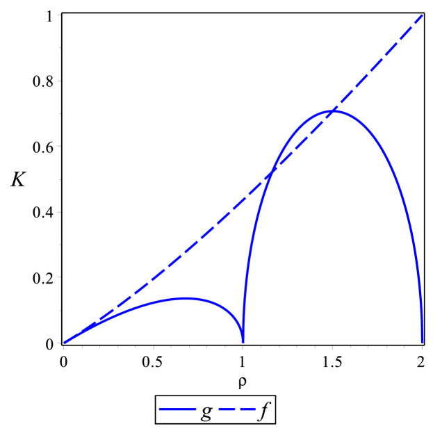
Figure 13: The graph of the function $g$ defined by (182) is superimposed to the graph of the function $f$ defined by (175).

1. For $K>g(\rho)$ we have eight generic critical points beside the two at the poles and four on the special meridians with $\vartheta_{2}=\pm\pi/2$, for a total of fourteen critical points. Four are maxima, four minima, and the remaining six are saddles.

2. For $K<g(\rho)$, we have a total of ten critical points, of which three are maxima, three minima, and the remaining four are saddles.

3. For $K=g(\rho)$, two different scenarios present themselves, according to whether $0<\rho<1$ or $1<\rho<2$. In the former case, the critical points are ten, whereas in the latter case they are twelve. In both cases, the total number of maxima is three, as many as the minima; only the number of saddles differs: there are four for $0<\rho<1$ and six for $1<\rho<2$. In the former case, two saddles are degenerate, but all four have index $\iota=-1$. In the latter case, two out of the six saddles are degenerate and have index $\iota=0$ (see Remark 16), while the remaining four are not degenerate and have the usual index $\iota=-1$.

4. A special note is deserved by the limiting values $\rho=1$ and $\rho=2$. For the former value, the total number of critical points is eight, whereas it is ten for the latter. For $\rho=1$, three maxima and three minima are accompanied by two degenerate saddles, each with index $\iota=-2$. For $\rho=2$, the same number of maxima and minima is accompanied by four degenerate saddles, each with index $\iota=-1$, for a total of ten critical points. The total number of critical points for both these limiting cases were predicted by our taxonomic analysis in Sect. 5.4: the case $\rho=1$ falls under row $(c_{2})$ in Table 2, while the case $\rho=2$ falls under row $(c)$ in Table 1.

We now describe in more detail how the different components of this varied landscape of critical points are combined together. The critical points for $K<g(\rho)$ are related to those for $K>g(\rho)$ in two different ways, corresponding to the two branches of $g$ in (182), according to whether $0<\rho<1$ or $1<\rho<2$.

For $0<\rho<1$, the four critical points on the special meridians $\vartheta_{2}=\pm\pi/2$ survive as $K$ decreases below $g(\rho)$; two saddles, one for each meridian, stay saddles, whereas a maximum on one meridian ($\vartheta_{2}=\pi/2$) becomes a saddle, as does a minimum on the other meridian ($\vartheta_{2}=-\pi/2$). On the other hand, always for $0<\rho<1$, two generic critical points, which are both saddles, approach each meridian $\vartheta_{2}=\pm\pi/2$ as $K$ approaches $g(\rho)$ from above; they coalesce for $K=g(\rho)$ on the extremal that on the targeted meridian will transform into a saddle, and disappear as $K<g(\rho)$. For $K=g(\rho)$, on each meridian $\vartheta_{2}=\pm\pi/2$ the coalesced critical point is a degenerate saddle with index $\iota=-1$.

For $1<\rho<2$, the evolution of critical points is somewhat different, though the final outcome is identical. As $K$ decreases below $g(\rho)$, the four critical points on meridians $\vartheta_{2}=\pm\pi/2$ cease to exist, but they do not mingle with the generic critical points, which instead survive. They rather annihilate in pairs on each meridian for $K=g(\rho)$. The superposition of a maximum with a saddle (for $\vartheta_{2}=\pi/2$) and that of a minimum with a saddle (for $\vartheta_{2}=-\pi/2$) give rise to a critical point with index $\iota=0$, so that for $K=g(\rho)$ and $1<\rho<2$ the total number of critical points is twelve: three maxima, three minima, and six saddles.

To determine the nature of the latter critical points, we expanded $\Psi_{or}$ in their vicinity. For $\vartheta_{2}=-\pi/2$ and $K=g(\rho)$, we found a degenerate saddle located at

$$\vartheta_{1}=\vartheta_{S}=-\arcsin\sqrt{\frac{\rho-1}{3-\rho}}$$ (183)

and we computed

$$\Psi_{or}(\vartheta_{1},\vartheta_{2}) = -\sqrt{(\rho-1)(3-\rho)}+12(2-\rho)\sqrt{\frac{\rho-1}{3-\rho}}\left(\vartheta_{2}+\frac{\pi}{2}\right)^{2}$$ (184)

$$+ \frac{1}{2}\sqrt{2(2-\rho)(3-\rho)}\left(\vartheta_{1}-\vartheta_{S}\right)^{3}$$

$$+ 3\sqrt{2}(5\rho-6)\sqrt{\frac{2-\rho}{3-\rho}}\left(\vartheta_{2}+\frac{\pi}{2}\right)^{2}\left(\vartheta_{1}-\vartheta_{S}\right)$$

$$+ O(4).$$

A similar formula applies to the degenerate saddle on the meridian $\vartheta_{2}=\pi/2$. It is then easy to conclude that both critical points are degenerate saddles with index $\iota=0$ (see, for example bolis:degenerate ). They migrate towards the poles as $\rho$ approaches $2$ along the line $K=g(\rho)$ and towards the Equator as $\rho$ approaches $1$. Correspondingly, the North Pole becomes a degenerate maximum (while the South Pole becomes a degenerate minimum) and the Equator hosts two symmetric “monkey saddles”.

7.7 Trivial symmetry $\{e\}$: the Bulk $\mathcal{B}$

We have so far discussed the critical strata that correspond to nontrivial symmetries in the cylinder $\mathsf{C}$ representing the parameter space of our theory.

The situation in the bulk $\mathcal{B}$ of the cylinder, i.e. for the generic case, has been discussed in detail in our previous work GV2016 ; there we have shown that – quite surprisingly – there are two generic octupolar phases, characterized by a different number (10 and 14) of critical points, and separated in parameter space by a separatrix. Moreover, one could also distinguish the cases where the maximum in the North Pole is the absolute one, and that where it is a local maximum but not the absolute one; these two regions are separated by a dome, having its vertex in one of the tetrahedral points $\mathcal{T}$ and meeting the disk $\mathcal{D}$ on the circle of radius $\rho=1$. This dome has been further investigated, providing more detailed information, in CQV . The generic incarnations of the octupolar potential below the dome in parameter space are illustrated in Figs. 14 and 15.

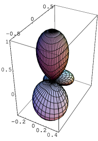
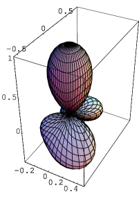
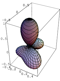
$K=0.1$	$K=0.2$	$K=0.3$
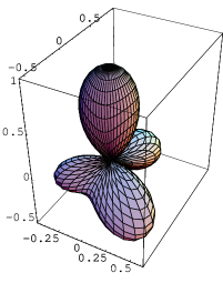
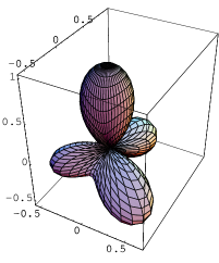
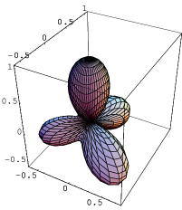
$K=0.4$	$K=0.5$	$K=0.6$

Figure 14: The potential for $\chi=\pi/3$ and $\rho=1/2$, for different values of $K>0$. We observe the transition from a phase with three maxima at low $K$ to a phase with four maxima at higher $K$. Generically, the potential is never reflection invariant through a vertical plane.

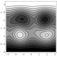
$K=0.1$	$K=0.2$	$K=0.3$
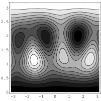
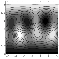
$K=0.4$	$K=0.5$	$K=0.6$

Figure 15: Same as Fig. 14 but with contour plots.

One easily distinguishes two different regions where the potential can be seen as topologically equivalent to the highly symmetric incarnations met on the disk $\mathcal{D}$ and at the tetrahedral points $\mathcal{T}$. In fact, the study of the generic configurations in the bulk, and of the separatrix between the two octupolar phases, was based on continuation techniques starting from these singular strata. Much of this study has already been presented in our previous work GV2016 ; CQV .

Here, the more detailed insight gained through the analysis of the highly symmetric cases $\chi=\pm\pi/2$ allows us to refine our understanding of the separatrix by establishing the existence of an extension where the total number of critical points for the octupolar potential is either 8 or 12, instead of the 10 that had already been found in GV2016 ; CQV .

Fig. 16 shows the outcome a standard numerical continuation technique applied to the sector $-\pi/2\leq\chi\leq-\pi/6$ in parameter space $(K,\rho,\chi)$, which in view of the symmetries described above is the only one bearing essential information. The educated eye will discern the graphs of functions $g$ anf $f$, plotted against $\rho$ upon the sections $\chi=-\pi/2$ and $\chi=-\pi/6$, respectively. The remaining curves outline the whole extended separatrix.

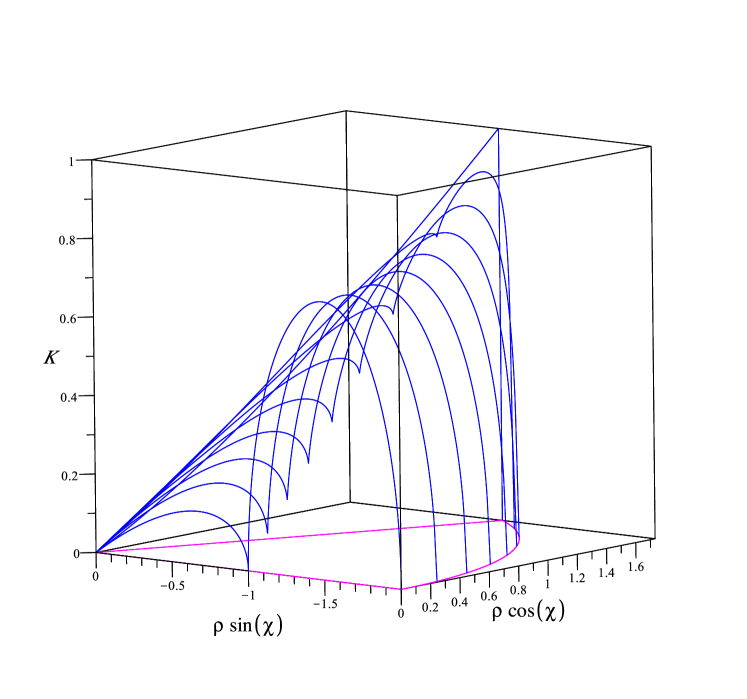
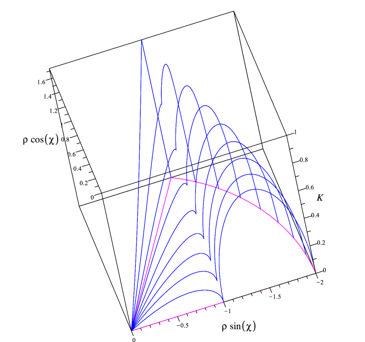
Figure 16: Two views of the whole separatrix, which is outlined by curves at equally spaced values of $\chi$ in the interval $[-{\pi}/{2},-{\pi}/{6}]$. A line of cusps, which bears 8 critical points for the octupolar potential, separates the inner component of the separatrix with 10 critical points from the outer component with 12 critical points.

A line of cusps connects the point $K=0$, $\rho=1$, $\chi=-\pi/2$ with the point $K=1$, $\rho=2$, $\chi=-\pi/6$: it bears 8 critical points for the octupolar potential. The line that connects the point $K=0$, $\rho=2$, $\chi=-\pi/2$ with the point $K=1$, $\rho=2$, $\chi=-\pi/6$ consists of an arc of circle of radius $2$ in the plane $K=0$ and a straight segment orthogonal to that plane: it bears instead 10 critical points. The bump delimited by these degenerate lines bears 12 critical points. Always, above the sepratrix the critical points are 14, whereas they are 10 below it. Our previous studies were confined to the cylinder $0\leq\rho\leq 1$, and so they were blind to the outer component of the sepratrix with 12 critical points for the octupolar potential.

7.8 Special transformations and potential invariance

Our choice of orientation and scaling allowed to simplify the potential, passing from seven to three parameters. This also reduced the allowed transformations. In fact, except at the special tetrahedral point $\rho=0,K=K_{0}$ (see above) we can only consider transformations which preserve the unit sphere and leave invariant the $z$ axis; we refer to these as oriented orthogonal transformations. They are just maps in $O(2)$ acting on the $(x,y)$ variables, and hence correspond to matrices of the form

$$M=\pmatrix{\cos\gamma&-s\sin\gamma\cr\sin\gamma&s\cos\gamma\cr},$$ (185)

where $s$ is just a sign, $s=\pm 1$ and corresponds to the determinant of $M$.

When we require invariance of $\Phi$ under such transformations, we obtain – by standard algebra – five classes of nontrivial solutions; each of these can exist only for certain values of the parameters, i.e. for certain regions $R$ in the parameter space. The results are summarized in Table 7 below. This table confirms that our classification of different phases is complete. In fact, the first class gives $G=O(2)$ in $\mathcal{C}$; the second one provides $G=D_{2h}$ in $\mathcal{D}$; the third ones provides $G=D_{3h}$ in $\mathcal{A}$, while the fourth points out at the fact that a symmetry $C_{3}$ is also present in $\mathcal{A}$; finally the fifth class shows that on the special planes $\mathcal{P}$ there is a reflection symmetry.

Table 7: Different oriented transformations as symmetries of the oriented potential in different regions $R$ of the parameter space. The symbol $-$ means that any value of the corresponding parameter is allowed.

$K$	$\rho$	$\chi$	$R$	$s$	$\gamma$
0	0	–	$\mathcal{C}$	$\pm 1$	–
0	–	–	$\mathcal{D}$	$-1$	$\pm\arccos(\pm\sin\chi)$
0	–	–	$\mathcal{D}$	$+1$	$\pm\pi$
–	0	–	$\mathcal{A}$	$-1$	$-5\pi/3$
–	0	–	$\mathcal{A}$	$-1$	$-\pi/2$
–	0	–	$\mathcal{A}$	$-1$	$-\pi/3$
–	0	–	$\mathcal{A}$	$-1$	$+\pi/3$
–	0	–	$\mathcal{A}$	$-1$	$+\pi/2$
–	0	–	$\mathcal{A}$	$-1$	$+5\pi/3$
–	0	–	$\mathcal{A}$	$+1$	$-\pi$
–	0	–	$\mathcal{A}$	$+1$	$-4\pi/3$
–	0	–	$\mathcal{A}$	$+1$	$-2\pi/3$
–	0	–	$\mathcal{A}$	$+1$	$+2\pi/3$
–	0	–	$\mathcal{A}$	$+1$	$+4\pi/3$
–	0	–	$\mathcal{A}$	$+1$	$+\pi$
–	–	$-5\pi/6$	$\mathcal{P}_{+}$	$\pm 1$	$\pi/3$
–	–	$-\pi/2$	$\mathcal{P}_{0}$	$\pm 1$	$\pi$
–	–	$-\pi/6$	$\mathcal{P}_{-}$	$\pm 1$	$-\pi/3$
–	–	$+\pi/6$	$\mathcal{P}_{+}$	$\pm 1$	$\pi/3$
–	–	$+\pi/2$	$\mathcal{P}_{0}$	$\pm 1$	$\pi$
–	–	$+5\pi/6$	$\mathcal{P}_{-}$	$\pm 1$	$-\pi/3$

8 Summary of critical points

In the following Table 8, we summarize our findings concerning critical points of the octupolar potential $\Phi$ in different regions of the admissible semi-definite cylinder $\mathsf{C}_{+}$ in parameter space. We preliminary leave out the critical points with index $\iota=0$, which we found on some special bifurcation loci. A more refined description of the landscape of critical points is outlined at the end of the section.

Table 8: Summary of the totality of critical points in parameter space with index $\iota\neq 0$, irrespective of all their possible additional features and characterization.

$G$	set	crit. pts.
$\{e\}$	$\mathcal{B}$	10 or 14
$D_{\infty h}$	$\mathcal{C}$	$2+\infty$
$D_{2h}$	$\mathcal{D}$	10
$D_{3h}$	$\mathcal{A}$	14
$T_{d}$	$\mathcal{T}$	14

The relations between geometric (and symmetry) strata of the cylinder are summarized in this diagram

$$\matrix{&&&&\mathcal{B}&&\cr&&&\swarrow&&\searrow&\cr&&\mathcal{A}&&&&\mathcal{D}\cr&\swarrow&&\searrow&&\swarrow&\cr\mathcal{T}&&&&\mathcal{C}&&\cr}$$

It should be noted that $\mathcal{C}$ and $\mathcal{T}$ can be reached from the bulk $\mathcal{B}$ also directly, i.e. without passing through $\mathcal{A}$ or $\mathcal{D}$.

Similarly, the relation between isotropy subgroups are summarized in the next diagram

$$\matrix{D_{\infty h}&&T_{d}&&D_{\infty h}\cr\downarrow&\swarrow&&\searrow&\downarrow\cr D_{3h}&&&&D_{2h}\cr&\searrow&&\swarrow&\cr&&\{e\}&&\cr}$$

Here we do not distinguish in $\mathcal{B}$ between the region $\mathcal{B}_{4}$ with four maxima of $\Psi_{or}$ from the region $\mathcal{B}_{3}$ with three maxima, as these correspond to different phases which do not differ in terms of symmetry. However, if we wish to classify the regions in $\mathsf{C}_{+}$ according to the cardinality of the real spectrum of the octupolar tensor ${\bf A}$ corresponding to $\Phi$ (which is the number of critical points of $\Phi$ on the unit sphere $S^{2}$), we need to be more refined. Then even the distinction between $\mathcal{B}_{3}$ and $\mathcal{B}_{4}$ is too gross.

We have shown that $\mathcal{B}_{3}$ and $\mathcal{B}_{4}$ are separated by a separatrix $\mathcal{S}$, a surface in parameter space which consists of two folds, $\mathcal{S}_{1}$ and $\mathcal{S}_{2}$, where $\Phi$ has 10 and 12 critical points, respectively. These subsurfaces are divided by a line of cusps $\mathcal{L}_{1}$ where $\Phi$ has 8 critical points. Moreover, $\mathcal{S}_{2}$ is bordered by another line, $\mathcal{L}_{2}$, where $\Phi$ has 10 critical points.

9 Conclusions

An octupolar tensor ${\bf A}$ is any third order, completely symmetric and completely traceless tensor. In 2D, ${\bf A}$ has the symmetries of an equilateral triangle and it can be effectively represented by a vector in the plane. In 3D, the symmetries enjoyed by ${\bf A}$ outline a much richer landscape. This paper has classified all of them by introducing the octupolar potential $\Phi$ associated with ${\bf A}$, that is, the cubic form of ${\bf A}$ restricted to the unit sphere $S^{2}$. The maxima (and antipodal minima) of $\Phi$ and their locations on the unit sphere describe the whole variety of octupolar tensors and allow for a visual representation of their symmetries.

We showed that a semi-indefinite cylinder $\mathsf{C}_{+}$ in a three-dimensional parameter space suffices to represent all possible incarnations of ${\bf A}$ in a three-dimensional physical space. Such a reduction (of the originally seven-dimensional parameter space) is obtained by fixing a maximum of $\Phi$ on the North Pole of $S^{2}$ and scaling its value to unity. We identified in $\mathsf{C}_{+}$ a number of special regions characterized by different symmetry groups for $\Phi$ and ordering of its maxima relative to the orienting maximum at the North Pole. For sake of illustration, each of these regions could be further divided in two subregions, which we distinguish by a ⁺ or a ^- superscript indicating where the maxima of $\Phi$ that supplement the orienting maximum have a larger or a smaller value than the latter.

The axis $\mathcal{A}$ of the cylinder $\mathsf{C}_{+}$ is characterized by a potential $\Phi$ enjoying the $D_{3h}$ symmetry, with $4$ maxima, $3$ of which are equal and either exceed the fourth, orienting maximum (in $\mathcal{A}^{+}$) or fall short of it (in $\mathcal{A}^{-}$). A special point of $\mathcal{A}$ separates $\mathcal{A}^{+}$ and $\mathcal{A}^{-}$: this is the only point with tetrahedral symmetry $T_{d}$, which, despite its singularity, has given its name to a whole class of bent-core liquid crystal phases.

On a disk $\mathcal{D}$, which is the base of $\mathsf{C}_{+}$, $\Phi$ has the $D_{2h}$ symmetry and possesses $3$ maxima. $\mathcal{D}$ can be separated into an inner disk $\mathcal{D}_{1}$ and an outer annulus $\mathcal{D}_{2}$. The center $\mathcal{C}$ of $\mathcal{D}$ has a special nature: there the potential $\Phi$ is axially symmetric. The symmetry group is $D_{\infty h}$ and the (primary) maximum at the North Pole is accompanied by a full circle of (secondary) maxima in the southern hemisphere of $S^{2}$.

Away from all these special loci is the generic bulk $\mathcal{B}$, where $\Phi$ has either $4$ (generically unequal) maxima (in $\mathcal{B}_{4}$) or $3$ (unequal) maxima (in $\mathcal{B}_{3}$), separated by a surface $\mathcal{S}$ in parameter space, called the separatrix. Both $\mathcal{B}_{3}$ and $\mathcal{B}_{4}$ (where, if necessary, we could distinguish the variants $\mathcal{B}_{3}^{\pm}$ and $\mathcal{B}_{4}^{\pm}$) enjoy three planes of symmetry, collectively denoted as $\mathcal{P}$. Correspondingly, $\Phi$ has on $S^{2}$ a reflection symmetry across a plane through the poles. Therefore, when the parameters fall in particular in $\mathcal{B}_{4}\cap\mathcal{P}$, two secondary maxima of $\Phi$ are equal.

Much like the decomposition of $\mathcal{D}$ into the union of $\mathcal{D}_{1}$ and $\mathcal{D}_{2}$, the separatrix $\mathcal{S}$ can be further decomposed into the union of two surfaces, an inner $\mathcal{S}_{1}$ and an outer $\mathcal{S}_{2}$, where $\Phi$ has 10 and 12 critical points, respectively. The boundary $\mathcal{L}_{1}$ of $\mathcal{S}_{1}$ is a line of cusps in parameter space where $\Phi$ has 8 critical points, whereas the outer boundary $\mathcal{L}_{2}$ of $\mathcal{S}_{2}$ is a line where $\Phi$ has 10 critical points.

All secondary maxima of $\Phi$ have a remarkable, universal feature, irrespective of the choice of parameters: they fall in the southern hemisphere of $S^{2}$, when the North Pole is marked by the primary, orienting maximum.

We trust that all the qualitative features of the octupolar potential described in this paper would prompt a better understanding of the many physical instances where an octupolar tensor is at play.

Appendix A The tetrahedron group

In this Appendix we give further detail – beyond those mentioned in Sect. 6 – on the tetrahedron group. We will work on a concrete realization of it in three-dimensional space; the points identifying the tetrahedron will be

$$\left(0,\frac{2\sqrt{2}}{3},-\frac{1}{3}\right),\ \left(\sqrt{\frac{2}{3}},-\frac{\sqrt{2}}{3},-\frac{1}{3}\right),\ \left(-\sqrt{\frac{2}{3}},-\frac{\sqrt{2}}{3},-\frac{1}{3}\right),\ \left(0,0,1\right).$$

In angular coordinates $(\vartheta_{1},\vartheta_{2})$, these are

$$\left(\theta_{0},-\frac{\pi}{2}\right),\ \left(\theta_{0},-\frac{\pi}{6}\right),\ \left(\theta_{0},\frac{5\pi}{6}\right),\ \left(\frac{\pi}{2},*\right),$$

where the symbol $*$ means that in this case $\vartheta_{2}$ is not determined, and

$$\theta_{0}=-\arcsin\left(\frac{1}{3}\right)\doteq-0.34.$$

The tetrahedron group $T_{d}\subset O(3)$ is made of $12$ matrices of determinant $+1$, associated to rotations of an angle $2\pi/3$ and multiples around each of the four axes of the tetrahedron, denoted as $T_{d}^{+}\subset SO(3)$; and other $12$ matrices of determinant $-1$, collectively denoted as $T_{d}^{-}$, among which are those associated to reflections through planes containing axes of the tetrahedron.

We now give the twelve matrices in $T_{d}^{+}$; these are:

$$\begin{array}[]{ll}M_{1}=\pmatrix{1&0&0\cr 0&1&0\cr 0&0&1\cr},&M_{2}=\pmatrix{-\frac{1}{2}&\frac{\sqrt{3}}{2}&0\cr-\frac{\sqrt{3}}{2}&-\frac{1}{2}&0\cr 0&0&1\cr},\\ M_{3}=\pmatrix{-\frac{1}{2}&-\frac{\sqrt{3}}{2}&0\cr\frac{\sqrt{3}}{2}&-\frac{1}{2}&0\cr 0&0&1\cr},&M_{4}=\pmatrix{\frac{1}{2}&\frac{\sqrt{3}}{2}&0\cr\frac{1}{2\sqrt{3}}&-\frac{1}{6}&\frac{2\sqrt{2}}{3}\cr\sqrt{\frac{2}{3}}&-\frac{\sqrt{2}}{3}&-\frac{1}{3}\cr},\\ M_{5}=\pmatrix{\frac{1}{2}&\frac{1}{2\sqrt{3}}&\sqrt{\frac{2}{3}}\cr\frac{\sqrt{3}}{2}&-\frac{1}{6}&-\frac{\sqrt{2}}{3}\cr 0&\frac{2\sqrt{2}}{3}&-\frac{1}{3}\cr},&M_{6}=\pmatrix{\frac{1}{2}&-\frac{\sqrt{3}}{2}&0\cr-\frac{1}{2\sqrt{3}}&-\frac{1}{6}&\frac{2\sqrt{2}}{3}\cr-\sqrt{\frac{2}{3}}&-\frac{\sqrt{2}}{3}&-\frac{1}{3}\cr},\\ M_{7}=\pmatrix{\frac{1}{2}&-\frac{1}{2\sqrt{3}}&-\sqrt{\frac{2}{3}}\cr-\frac{\sqrt{3}}{2}&-\frac{1}{6}&-\frac{\sqrt{2}}{3}\cr 0&\frac{2\sqrt{2}}{3}&-\frac{1}{3}\cr},&M_{8}=\pmatrix{-\frac{1}{2}&\frac{1}{2\sqrt{3}}&\sqrt{\frac{2}{3}}\cr-\frac{1}{2\sqrt{3}}&\frac{5}{6}&-\frac{\sqrt{2}}{3}\cr-\sqrt{\frac{2}{3}}&-\frac{\sqrt{2}}{3}&-\frac{1}{3}\cr},\\ M_{9}=\pmatrix{-\frac{1}{2}&-\frac{1}{2\sqrt{3}}&-\sqrt{\frac{2}{3}}\cr\frac{1}{2\sqrt{3}}&\frac{5}{6}&-\frac{\sqrt{2}}{3}\cr\sqrt{\frac{2}{3}}&-\frac{\sqrt{2}}{3}&-\frac{1}{3}\cr},&M_{10}=\pmatrix{0&\frac{1}{\sqrt{3}}&-\sqrt{\frac{2}{3}}\cr\frac{1}{\sqrt{3}}&-\frac{2}{3}&-\frac{\sqrt{2}}{3}\cr-\sqrt{\frac{2}{3}}&-\frac{\sqrt{2}}{3}&-\frac{1}{3}\cr},\\ M_{11}=\pmatrix{0&-\frac{1}{\sqrt{3}}&\sqrt{\frac{2}{3}}\cr-\frac{1}{\sqrt{3}}&-\frac{2}{3}&-\frac{\sqrt{2}}{3}\cr\sqrt{\frac{2}{3}}&-\frac{\sqrt{2}}{3}&-\frac{1}{3}\cr},&M_{12}=\pmatrix{-1&0&0\cr 0&\frac{1}{3}&\frac{2\sqrt{2}}{3}\cr 0&\frac{2\sqrt{2}}{3}&-\frac{1}{3}\cr}.\end{array}$$

The multiplication table for these matrices is the following:

$$P_{11}=\left(\begin{array}[]{llllllllllll}1&2&3&4&5&6&7&8&9&10&11&12\\ 2&3&1&11&7&8&12&10&4&6&9&5\\ 3&1&2&9&12&10&5&6&11&8&4&7\\ 4&12&6&5&1&11&9&2&10&7&3&8\\ 5&8&11&1&4&3&10&12&7&9&6&2\\ 6&4&12&10&8&7&1&11&3&2&5&9\\ 7&10&9&2&11&1&6&5&12&4&8&3\\ 8&11&5&6&10&12&2&9&1&3&7&4\\ 9&7&10&12&3&4&11&1&8&5&2&6\\ 10&9&7&8&6&5&3&4&2&1&12&11\\ 11&5&8&7&2&9&4&3&6&12&1&10\\ 12&6&4&3&9&2&8&7&5&11&10&1\end{array}\right).$$

These generate several subgroups; in particular – apart from the trivial ones consisting of $M_{1}$ alone and of the full group $T_{d}^{+}$ – we have four subgroups of order three,

$$G_{1}=\{M_{1},M_{2},M_{3}\},\ G_{2}=\{M_{1},M_{4},M_{5}\},\ G_{3}=\{M_{1},M_{6},M_{7}\},\ G_{4}=\{M_{1},M_{8},M_{9}\};$$

three groups of order two,

$$G_{5}=\{M_{1},M_{10}\},\ G_{6}=\{M_{1},M_{11}\},\ G_{7}=\{M_{1},M_{12}\};$$

and one group of order four,

$$G_{8}=\{M_{1},M_{10},M_{11},M_{12}\}.$$

The latter is the only nontrivial normal subgroup, and also the only one acting freely.

We can also easily determine the subspaces $F_{k}$ admitting each of these $G_{k}$ as symmetry subgroups; in particular,

$$F_{1}=(0,0,z),\ F_{2}=(\sqrt{6}z,\sqrt{2}z,z),\ F_{3}=(-\sqrt{6}z,\sqrt{2}z,z),\ F_{4}=(0,-2\sqrt{2}z,z);$$

the subgroups $G_{k}$, $k=1,2,3,4$ act as rotations (by an angle $2\pi/3$) around these axes, which are just the axes of the tetrahedron. Moreover,

$$F_{5}=\left(-\sqrt{\frac{3}{2}}z,-\sqrt{\frac{1}{2}}z,z\right),\ F_{6}=\left(\sqrt{\frac{3}{2}}z,-\sqrt{\frac{1}{2}}z,z\right),\ F_{7}=\left(0,\sqrt{2}z,z\right);$$

these subgroups $G_{k}$, $k=5,6,7$, represent rotations by $\pi$ around the given axes $F_{k}$. Note that $F_{8}=\{(0,0,0)\}$, and correspondingly $G_{8}$ represents combined $\pi$ rotations around the $F_{5},F_{6},F_{7}$ axes.

We can give as well the twelve matrices in $T_{d}^{-}$; these are:

$$\begin{array}[]{ll}M_{1}^{-}=\pmatrix{-1&0&0\cr 0&1&0\cr 0&0&1\cr},&M_{2}^{-}=\pmatrix{\frac{1}{2}&-\frac{\sqrt{3}}{2}&0\cr-\frac{\sqrt{3}}{2}&-\frac{1}{2},0\cr 0&0&1\cr},\\ M_{3}^{-}=\pmatrix{\frac{1}{2}&\frac{\sqrt{3}}{2}&0\cr\frac{\sqrt{3}}{2}&-\frac{1}{2},0\cr 0&0&1\cr},&M_{4}^{-}=\pmatrix{-\frac{1}{2}&-\frac{\sqrt{3}}{2}&0\cr\frac{1}{2\sqrt{3}}&-\frac{1}{6}&\frac{2\sqrt{2}}{3}\cr\sqrt{\frac{2}{3}}&-\frac{\sqrt{2}}{3}&-\frac{1}{3}\cr},\\ M_{5}^{-}=\pmatrix{-\frac{1}{2}&-\frac{1}{2\sqrt{3}}&-\sqrt{\frac{2}{3}}\cr\frac{\sqrt{3}}{2}&-\frac{1}{6}&-\frac{\sqrt{2}}{3}\cr 0&\frac{2\sqrt{2}}{3}&-\frac{1}{3}\cr},&M_{6}^{-}=\pmatrix{-\frac{1}{2}&\frac{\sqrt{3}}{2}&0\cr-\frac{1}{2\sqrt{3}}&-\frac{1}{6}&\frac{2\sqrt{2}}{3}\cr-\sqrt{\frac{2}{3}}&-\frac{\sqrt{2}}{3}&-\frac{1}{3}\cr},\\ M_{7}^{-}=\pmatrix{-\frac{1}{2}&\frac{1}{2\sqrt{3}}&\sqrt{\frac{2}{3}}\cr-\frac{\sqrt{3}}{2}&-\frac{1}{6}&-\frac{\sqrt{2}}{3}\cr 0,\frac{2\sqrt{2}}{3}&-\frac{1}{3}\cr},&M_{8}^{-}=\pmatrix{\frac{1}{2}&-\frac{1}{2\sqrt{3}}&-\sqrt{\frac{2}{3}}\cr-\frac{1}{2\sqrt{3}}&\frac{5}{6}&-\frac{\sqrt{2}}{3}\cr-\sqrt{\frac{2}{3}}&-\frac{\sqrt{2}}{3}&-\frac{1}{3}\cr},\\ M_{9}^{-}=\pmatrix{\frac{1}{2}&\frac{1}{2\sqrt{3}}&\sqrt{\frac{2}{3}}\cr\frac{1}{2\sqrt{3}}&\frac{5}{6}&-\frac{\sqrt{2}}{3}\cr\sqrt{\frac{2}{3}}&-\frac{\sqrt{2}}{3}&-\frac{1}{3}\cr},&M_{10}^{-}=\pmatrix{0&-\frac{1}{\sqrt{3}}&\sqrt{\frac{2}{3}}\cr\frac{1}{\sqrt{3}}&-\frac{2}{3}&-\frac{\sqrt{2}}{3}\cr-\sqrt{\frac{2}{3}}&-\frac{\sqrt{2}}{3}&-\frac{1}{3}\cr},\\ M_{11}^{-}=\pmatrix{0&\frac{1}{\sqrt{3}}&-\sqrt{\frac{2}{3}}\cr-\frac{1}{\sqrt{3}}&-\frac{2}{3}&-\frac{\sqrt{2}}{3}\cr\sqrt{\frac{2}{3}}&-\frac{\sqrt{2}}{3}&-\frac{1}{3}\cr},&M_{12}^{-}=\pmatrix{1&0&0\cr 0&\frac{1}{3}&\frac{2\sqrt{2}}{3}\cr 0&\frac{2\sqrt{2}}{3}&-\frac{1}{3}\cr}.\end{array}$$

Once $M_{1}^{-}$ has been defined, they are built by

$$M_{k}^{-}=M_{1}^{-}M_{k}.$$

It is obvious that $M_{1}^{-}$ represents a reflection (across the $(y,z)$ plane), so that the matrices $M_{k}^{-}$ represent the combination of rotations and reflections.

If we write $M_{k+12}=M_{k}^{-}$, the full multiplication table is given in block form by

$$P=\pmatrix{P_{11}&P_{12}\cr P_{21}&P_{22}\cr},$$

where $P_{11}$ has been given above, and the other blocks are:

$$P_{12}=\left(\begin{array}[]{llllllllllll}13&14&15&16&17&18&19&20&21&22&23&24\\ 15&13&14&21&24&22&17&18&23&20&16&19\\ 14&15&13&23&19&20&24&22&16&18&21&17\\ 18&16&24&22&20&19&13&23&15&14&17&21\\ 19&22&21&14&23&13&18&17&24&16&20&15\\ 16&24&18&17&13&23&21&14&22&19&15&20\\ 17&20&23&13&16&15&22&24&19&21&18&14\\ 21&19&22&24&15&16&23&13&20&17&14&18\\ 20&23&17&18&22&24&14&21&13&15&19&16\\ 23&17&20&19&14&21&16&15&18&24&13&22\\ 22&21&19&20&18&17&15&16&14&13&24&23\\ 24&18&16&15&21&14&20&19&17&23&22&13\end{array}\right),$$

$$P_{21}=\left(\begin{array}[]{llllllllllll}13&14&15&16&17&18&19&20&21&22&23&24\\ 14&15&13&23&19&20&24&22&16&18&21&17\\ 15&13&14&21&24&22&17&18&23&20&16&19\\ 16&24&18&17&13&23&21&14&22&19&15&20\\ 17&20&23&13&16&15&22&24&19&21&18&14\\ 18&16&24&22&20&19&13&23&15&14&17&21\\ 19&22&21&14&23&13&18&17&24&16&20&15\\ 20&23&17&18&22&24&14&21&13&15&19&16\\ 21&19&22&24&15&16&23&13&20&17&14&18\\ 22&21&19&20&18&17&15&16&14&13&24&23\\ 23&17&20&19&14&21&16&15&18&24&13&22\\ 24&18&16&15&21&14&20&19&17&23&22&13\end{array}\right),$$

$$P_{22}=\left(\begin{array}[]{llllllllllll}1&2&3&4&5&6&7&8&9&10&11&12\\ 3&1&2&9&12&10&5&6&11&8&4&7\\ 2&3&1&11&7&8&12&10&4&6&9&5\\ 6&4&12&10&8&7&1&11&3&2&5&9\\ 7&10&9&2&11&1&6&5&12&4&8&3\\ 4&12&6&5&1&11&9&2&10&7&3&8\\ 5&8&11&1&4&3&10&12&7&9&6&2\\ 9&7&10&12&3&4&11&1&8&5&2&6\\ 8&11&5&6&10&12&2&9&1&3&7&4\\ 11&5&8&7&2&9&4&3&6&12&1&10\\ 10&9&7&8&6&5&3&4&2&1&12&11\\ 12&6&4&3&9&2&8&7&5&11&10&1\end{array}\right).$$

We now have subgroups involving elements of both $T_{d}^{+}$ and $T_{d}^{-}$; in particular, using again the 1 through 24 numeration and denoting $M_{k}$ directly by $k$, we have the following subgroups; those of types $\mathcal{G}_{a}$ through $\mathcal{G}_{c}$ extending those seen above, while those of type $\mathcal{G}_{d}$ involve no other element of $T_{d}^{+}$ but the identity:

$$\mathcal{G}_{a}: (1,2,3,13,14,15),(1,2,3,16,21,23),(1,2,3,17,19,24),(1,2,3,18,20,22);$$

$$(1,4,5,13,18,19),(1,4,5,14,16,22),(1,4,5,15,21,24),(1,4,5,17,20,23);$$

$$(1,8,9,13,20,21),(1,8,9,14,19,23),(1,8,9,15,17,22),(1,8,9,16,18,24);$$

$$\mathcal{G}_{b}: (1,10,13,23),(1,10,14,17),(1,10,15,20),(1,10,16,19),(1,10,18,21),(1,10,22,24);$$

$$(1,11,13,22),(1,11,14,21),(1,11,15,19),(1,11,16,20),(1,11,17,18),(1,11,23,24);$$

$$(1,12,13,24),(1,12,14,18),(1,12,15,16),(1,12,17,21),(1,12,19,20),(1,12,22,23);$$

$$\mathcal{G}_{c}: (1,10,11,12,13,22,23,24),(1,10,11,12,14,17,18,21),(1,10,11,12,15,16,19,20);$$

$$\mathcal{G}_{d}: (1,13),(1,14),(1,15),(1,20),(1,21),(1,24).$$

Groups of type $\mathcal{G}_{a}$ contain rotations by $2\pi/3$ around an axis and reflections through a plane containing that axis, hence they are of type $D_{3h}$, and only the first one leaves the distinguished point at the North Pole untouched; those of type $\mathcal{G}_{b}$ contain rotations by $\pi$ around an axis and reflections through a plane containing that axis, hence are of type $D_{2h}$, but none of these leaves the distinguished point at the North Pole untouched; those of type $\mathcal{G}_{c}$ combine rotations and reflections through different axes, and none of them preserves the North Pole; and those of type $\mathcal{G}_{d}$ consist just of reflections in a plane, hence are of type $D_{h}$; the first three preserve the North Pole.

References

• (1) Ashcroft, N.W., Mermin, D.N.: Solid State Physics. Academic Press, Saunders College (1976)
• (2) Bolis, T.S.: Degenerate critical points. Math. Mag. 53(5), 294–299 (1980)
• (3) Boyd, R.W.: Nonlinear Optics, 3rd edn. Academic Press, Burlington, MA 01803, USA (2008)
• (4) Buckingham, A.D.: Angular correlation in liquids. Discuss. Faraday Soc. 43, 205–211 (1967)
• (5) Cartwright, D., Sturmfels, B.: The number of eigenvalues of a tensor. Linear Algebra Appl. 438(2), 942–952 (2013)
• (6) Chen, Y., Qi, L., Virga, E.G.: Octupolar tensors for liquid crystals. J. Phys. A: Math. Theor. 51(2), 025206 (2018)
• (7) Cicogna, G.: Symmetry breakdown from bifurcation. Lett. Nuovo Cimento (1971-1985) 31, 600–602 (1981)
• (8) Cicogna, G.: A nonlinear version of the equivalent bifurcation lemma. J. Phys. A 23, L1339–L1343 (1990)
• (9) Coleman, B.D., Markovitz, H., Noll, W.: Viscometric Flows of Non-Newtonian Fluids, Theory and Experiment, Springer Tracts in Natural Philosophy, vol. 5. Springer-Verlag, Berlin (1966)
• (10) Dailey, C.A., Burke, B.J., Simpson, G.J.: The general failure of Kleinman symmetry in practical nonlinear optical applications. Chem. Phys. Lett. 390(1), 8–13 (2004)
• (11) Fel, L.G.: Symmetry of the Fréedericksz transition in nonchiral nematic liquid crystals. Phys. Rev. E 52, 2692–2701 (1995)
• (12) Fel, L.G.: Tetrahedral symmetry in nematic liquid crystals. Phys. Rev. E 52, 702–717 (1995)
• (13) Gaeta, G.: Reduction and equivariant branching lemma: Dynamical systems, evolution PDEs, and gauge theories. Acta Appl. Math. 28, 43–68 (1992)
• (14) Gaeta, G., Virga, E.G.: Octupolar order in three dimensions. Eur. Phys. J. E 39, 113 (2016)
• (15) de Gennes, P., Prost, J.: The Physics of Liquid Crystals. Oxford University Press, Oxford, UK (1993)
• (16) Gramsbergen, E.F., Longa, L., de Jeu, W.H.: Landau theory of the nematic-isotropic phase transition. Phys. Rep. 135(4), 195–257 (1986)
• (17) Hamermesh, M.: Group Theory and its Application to Physical Problems. Dover, Mineola, NY, 11501, USA (1989)
• (18) Kanis, D.R., Ratner, M.A., Marks, T.J.: Design and construction of molecular assemblies with large second-order optical nonlinearities. Quantum chemical aspects. Chem. Rev. 94, 195–242 (1994)
• (19) Kittel, C.: Introduction to Solid State Physics. Wiley, New York (1996)
• (20) Kleinman, D.A.: Nonlinear dielectric polarization in optical media. Phys. Rev. 126, 1977–1979 (1962)
• (21) Landau, L.D.: The theory of phase transitions. Nature 138, 840–841 (1936)
• (22) Landau, L.D.: On the theory of phase transitions I. Zh. Exsp. Teor. Fiz. 7, 19–32 (1937)
• (23) Landau, L.D., Lifshitz, E.M.: Statistical Physics. Pergamon Press, Oxford, UK (1958)
• (24) Landau, L.D., Lifshitz, E.M.: Quantum Mechanics. Pergamon Press, Oxford, UK (1965)
• (25) Liu, K., Greitemann, J., Pollet, L.: Generic first-order phase transitions between isotropic and orientational phases with polyhedral symmetries. Phys. Rev. E 97, 012706 (2018)
• (26) Liu, K., Nissinen, J., Nussinov, Z., Slager, R.J., Wu, K., Zaanen, J.: Classification of nematic order in 2 + 1 dimensions: Dislocation melting and $o$(2)/${Z}_{N}$ lattice gauge theory. Phys. Rev. B 91, 075103 (2015)
• (27) Liu, K., Nissinen, J., Slager, R.J., Wu, K., Zaanen, J.: Generalized liquid crystals: Giant fluctuations and the vestigial chiral order of $i$, $o$, and $t$ matter. Phys. Rev. X 6, 041025 (2016)
• (28) Lubensky, T.C., Radzihovsky, L.: Theory of bent-core liquid-crystal phases and phase transitions. Phys. Rev. E 66, 031704 (2002)
• (29) Ni, G., Qi, L., Wang, F., Wang, Y.: The degree of the e-characteristic polynomial of an even order tensor. J. Math. Anal. Appl. 329(2), 1218–1229 (2007)
• (30) Noll, W.: Finite-Dimensional Spaces: Algebra, Geometry, and Analysis, Mechanics: Analysis, vol. 10. Martinus Nijhoff, Dordrecht (1987)
• (31) Peliti, L.: Statistical Mechanics in a Nutshell. Princeton University Press, Princeton, NJ, USA (2011)
• (32) Qi, L.: Eigenvalues of a real supersymmetric tensor. J. Symbolic Comput. 40(6), 1302–1324 (2005)
• (33) Qi, L.: Rank and eigenvalues of a supersymmetric tensor, the multivariate homogeneous polynomial and the algebraic hypersurface it defines. J. Symbolic Comput. 41(12), 1309–1327 (2006)
• (34) Qi, L.: Eigenvalues and invariants of tensors. J. Math. Anal. Appl. 325(2), 1363–1377 (2007)
• (35) Qi, L., Chen, H., Chen, Y.: Tensor Eigenvalues and Their Applications, Advances in Mechanics and Mathematics, vol. 39. Springer Nature, Singapore (2018)
• (36) Röhrl, H.: Algebras and differential equations. Nagoya Math. J. 68, 59–122 (1977)
• (37) Röhrl, H.: A theorem on non-associative algebras and its application to differential equations. Manuscripta Mathematica 21(2), 181–187 (1977)
• (38) Saupe, A.: Disclinations and properties of the directorfield in nematic and cholesteric liquid crystals. Mol. Cryst. Liq. Cryst. 21, 211–238 (1973)
• (39) Sonnet, A.M., Virga, E.G.: Reorientational dynamics of conjugated nematic point defects. Liq. Cryst. 37, 785–797 (2010)
• (40) Stewart, I.W.: The Static and Dynamic Continuum Theory of Liquid Crystals. Taylor & Francis (2004)
• (41) Stoker, J.J.: Differential Geometry, Pure and Applied Mathematics, vol. XX. Wiley-Interscience, New York (1969)
• (42) Tang, X., Selinger, J.V.: Orientation of topological defects in 2D nematic liquid crystals. Soft Matter 13, 5481–5490 (2017)
• (43) Tolédano, P., Dmitriev, V.: Reconstructive Phase Transitions in Crystals and Quasicrystals. World Scientific, Singapore (1996)
• (44) Truesdell, C.A.: A First Course in Rational Continuum Mechanics. Academic Press, Boston (1977). A second edition, corrected, revised, and augmented, was published by the same Publisher in 1991.
• (45) Turzi, S.S.: On the Cartesian definition of orientational order parameters. J. Math. Phys. 52(5), 053517 (2011)
• (46) Vanderbauwhede, A.: Local Bifurcation and Symmetry. Pitman, Boston (1982)
• (47) Virga, E.G.: Variational Theories for Liquid Crystals. Chapman & Hall, London (1994)
• (48) Virga, E.G.: Octupolar order in two dimensions. Eur. Phys. J. E 38(6), 1–7 (2015)
• (49) Vromans, A.J., Giomi, L.: Orientational properties of nematic disclinations. Soft Matter 12, 6490–6495 (2016)
• (50) Walcher, S.: Algebras and Differential Equations. Hadronic Press, Palm Harbor, FL, 34684, USA (1991)
• (51) Walcher, S.: Eigenvectors of tensors (2017). Talk given at GSD2017 Conference.
• (52) Walcher, S.: Eigenvectors of tensors – A primer (2018). Preprint.
• (53) Wergifosse, M., Liégeois, V., Champagne, B.: Evaluation of the molecular static and dynamic first hyperpolarizabilities. Int. J. Quantum Chem. 114(14), 900–910
• (54) Zyss, J., Ledoux, I.: Nonlinear optics in multipolar media: theory and experiments. Chem. Rev. 94(1), 77–105 (1994)