Traveling waves for some nonlocal 1D Gross–Pitaevskii equations with nonzero conditions at infinity

Abstract

We consider a nonlocal family of Gross–Pitaevskii equations with nonzero conditions at infinity in dimension one. We provide conditions on the nonlocal interaction such that there is a branch of traveling waves solutions with nonvanishing conditions at infinity. Moreover, we show that the branch is orbitally stable. In this manner, this result generalizes known properties for the contact interaction given by a Dirac delta function. Our proof relies on the minimization of the energy at fixed momentum.

As a by-product of our analysis, we provide a simple condition to ensure that the solution to the Cauchy problem is global in time.

Keywords: Nonlocal Schrödinger equation, Gross–Pitaevskii equation, traveling waves, dark solitons, orbital stability, nonzero conditions at infinity

2010 Mathematics Subject Classification: 35Q55; 35J20; 35C07; 35B35; 37K05; 35C08; 35Q53

1 Introduction

1.1 The problem

We consider the one-dimensional nonlocal Gross–Pitaevskii equation for $\Psi:\mathbb{R}\times\mathbb{R}\to\mathbb{C}$ introduced by Gross [40] and Pitaevskii [56] to describe a Bose gas

$$i\partial_{t}\Psi={\partial_{xx}\Psi}+\Psi(\mathcal{W}*(1-|\Psi|^{2}))\quad\text{ in }\leavevmode\nobreak\ \mathbb{R}\times\mathbb{R},$$ (NGP)

with the boundary condition at infinity

$$\lim_{|x|\to\infty}|\Psi|=1.$$ (1)

Here $*$ denotes the convolution in $\mathbb{R}$, and $\mathcal{W}$ is a real-valued even distribution that describes the interaction between particles. The nonzero boundary condition (1) arises as a background density. This model appears naturally in several areas of quantum physics, for instance in the description of superfluids [8, 1] and in optics when dealing with thermo-optic materials because the thermal nonlinearity is usually highly nonlocal [59]. An important property of equation (NGP) with the boundary condition at infinity (1), is that it allows to study dark solitons, i.e.  localized density notches that propagate without spreading [43], that have been observed for example in Bose-Einstein condensates [32, 6].

There have been extensive studies concerning the dynamics of equation (NGP), and the existence and stability of traveling waves in the case of the contact interaction $\mathcal{W}=\delta_{0}$ (see [16, 11, 15, 14, 25, 24, 35, 51, 27, 42, 41, 44] and the references therein). However, there are very few mathematical results concerning general nonlocal interactions with nonzero conditions at infinity. In [28, 55] the authors gave conditions on $\mathcal{W}$ to get global well-posedness of the equation and in [29] conditions were established for the nonexistence of traveling waves (in higher dimensions). Nevertheless, to our knowledge, there is no result concerning the existence of localized solutions to (NGP) when $\mathcal{W}$ is not given by a Dirac delta. The aim of this paper is to provide conditions on $\mathcal{W}$ in order to have stable finite energy traveling wave solutions, more commonly refereed to as dark solitons due to the nonzero boundary condition (1). More precisely, we look for a solution of the form

$$\Psi_{c}(x,t)=u(x-ct),$$

representing a traveling wave propagating at speed $c$. Hence, the profile $u$ satisfies the nonlocal ODE

$$icu^{\prime}+u^{\prime\prime}+u(\mathcal{\mathcal{W}}*(1-|u|^{2}))=0\quad\text{ in }\mathbb{R}.$$ (TW_W,c)

By taking the conjugate of the function, we assume without loss of generality that $c\geq 0$.

Let us remark that when considering vanishing boundary conditions at infinity, this kind of equation has been studied extensively [37, 21, 54] and long-range dipolar interactions in condensates have received recently much attention [45, 20, 4, 7, 50]. However, the techniques used in these works cannot be adapted to include solutions satisfying (1).

We recall that (NGP) is Hamiltonian and its energy

$$E(\Psi(t))=\frac{1}{2}\int_{\mathbb{R}}|\partial_{x}\Psi(t)|^{2}\,dx+\frac{1}{4}\int_{\mathbb{R}}(W*(1-|\Psi(t)|^{2}))(1-|\Psi(t)|^{2})\,dx,$$

is formally conserved, as well as the (renormalized) momentum

$$p(\Psi(t))=\int_{\mathbb{R}}\langle i\partial_{x}\Psi^{\prime}(t),\Psi(t)\rangle\left(1-\frac{1}{|\Psi(t)|^{2}}\right)dx,$$

at least as $\inf_{x\in\mathbb{R}}|\Psi(x,t)|>0$, where $\langle z_{1},z_{2}\rangle=\operatorname{Re}(z_{1}\bar{z}_{2})$, for $z_{1}$, $z_{2}\in\mathbb{C}$ (see [27, 17]). In this manner, we seek nontrivial solutions of (TW_W,c) in the energy space

$$\mathcal{E}(\mathbb{R})=\{v\in H^{1}_{\operatorname{loc}}(\mathbb{R}):1-|v|^{2}\in L^{2}(\mathbb{R}),\ v^{\prime}\in L^{2}(\mathbb{R})\},$$

and more precisely in the nonvanishing energy space

$$\mathcal{N}\mathcal{E}(\mathbb{R})=\{v\in\mathcal{E}(\mathbb{R}):\inf_{\mathbb{R}}|v|>0\},$$

where the momentum will be well defined. It is simple to check, using the Morrey inequality, that the functions in $\mathcal{E}(\mathbb{R})$ are uniformly continuous and satisfy $\lim_{|x|\to\infty}|v(x)|=1$.

When $\mathcal{W}$ is given by a Dirac delta function, equation (TW${}_{\delta_{0},c}$) corresponds to the classical Gross–Pitaevskii equation, which can be solved explicitly. As explained in [10], if $c\geq\sqrt{2}$ the only solutions in $\mathcal{E}(\mathbb{R})$ are the trivial ones (i.e. the constant functions of modulus one) and if $0\leq c<\sqrt{2}$, the nontrivial solutions are given, up to invariances (translations and a multiplications by constants of modulus one), by

$$u_{c}(x)=\sqrt{\frac{2-c^{2}}{2}}\tanh\left(\frac{\sqrt{2-c^{2}}}{2}x\right)-i\frac{c}{\sqrt{2}}.$$ (2)

Thus there is a family of dark solitons belonging to $\mathcal{N}\mathcal{E}(\mathbb{R})$ for $c\in(0,\sqrt{2})$ and there is one stationary black soliton associated with the speed $c=0$. Notice also that the values of $u_{c}(\infty)$ and $u_{c}(-\infty)$ are different, and thus we cannot relax the condition (1) to $\lim_{|x|\to\infty}{\Psi}=1$, as is usually done in higher dimensions.

The study of equation (TW${}_{\delta_{0},c}$) can be generalized to other types of local nonlinearities such as the cubic-quintic nonlinearity and some cubic-quintic-septic nonlinearities as shown in [23, 53]. The techniques used by the authors rely on the analysis of a second-order ODE of Newton type, so that the Cauchy–Lipschitz theorem can be invoked and some explicit formulas can be deduced. These arguments cannot be applied to (TW_W,c) due to the nonlocal interaction. For this reason, our approach to show existence of traveling waves relies on a priori energy estimates and a concentration-compactness argument, that allow us to prove that there are functions that minimize the energy at fixed momentum. These minimizers are solutions to (TW_W,c) and we can also establish that they are orbitally stable (see Theorem 4). These kinds of arguments have been used by several authors to establish existence of solitons for the (local) Gross–Pitaevskii equation in higher dimensions and for some related equations with zero conditions at infinity (see e.g. [11, 51, 25, 49, 52, 5, 46]). The main difficulty in our case is to handle the nonvanishing conditions at infinity, the fact that the constraint given by the momentum is not a homogeneous function along with the nonlocal interactions.

1.2 The critical speed and assumptions on $\mathcal{W}$

Linearizing equation (NGP) around the constant solution equal to 1 and imposing $e^{i(\xi x-wt)}$ as a solution of the resulting equation, we obtain the dispersion relation

$$w(\xi)=\sqrt{\xi^{4}+2\widehat{\mathcal{W}}(\xi)\xi^{2}},$$ (3)

where $\widehat{\mathcal{W}}$ denotes the Fourier transform of $\mathcal{W}$. Supposing that $\widehat{\mathcal{W}}$ is positive and continuous at the origin, we get the so-called speed of sound

$$c_{*}(\mathcal{W})=\lim_{\xi\to 0}\frac{w(\xi)}{\xi}=\sqrt{2\widehat{\mathcal{W}}(0)}.$$

The dispersion relation (3) was first observed by Bogoliubov [18] in the study of a Bose–Einstein gas. He then argued that the gas should move with a speed less than $c_{*}(\mathcal{W})$ to preserve its superfluid properties. This leads to the conjecture that there is no nontrivial solution of (TW_W,c) with finite energy when $c>c_{*}(\mathcal{W})$. Actually, one of the authors proved this conjecture in [29] in dimensions greater than one, under some conditions on $\mathcal{W}$.

In order to simplify our computations, we can normalize the equation so that the critical speed is fixed. Indeed, it is easy to verify that the rescaling $x\mapsto x/\widehat{\mathcal{W}}(0)^{1/2}$ and $t\mapsto t/\widehat{\mathcal{W}}(0)$ allows us to replace $\widehat{\mathcal{W}}(\xi)$ by $\widehat{\mathcal{W}}(\xi)/\widehat{\mathcal{W}}(0)$ in (NGP). Therefore, we assume from now on that $\widehat{\mathcal{W}}(0)=1$ and hence that the critical speed is

$$c_{*}=\sqrt{2}.$$

Before going any further, let us state the assumptions that we need on $\mathcal{W}$.

1. $\mathcal{W}$ is an even tempered distribution with $\widehat{\mathcal{W}}\in L^{\infty}(\mathbb{R})$, and $\widehat{\mathcal{W}}\geq 0$ a.e. on $\mathbb{R}$. Moreover $\widehat{\mathcal{W}}$ is continuous at the origin and $\widehat{\mathcal{W}}(0)=1$.

2. $\widehat{\mathcal{W}}$ belongs to $C_{b}^{3}(\mathbb{R})$, $(\widehat{\mathcal{W}})^{\prime\prime}(0)>-1$ and $\widehat{\mathcal{W}}(\xi)\geq 1-\xi^{2}/2$, for all $|\xi|<2.$

3. $\widehat{\mathcal{W}}$ admits a meromorphic extension to the upper half-plane $\mathbb{H}:=\{z\in\mathbb{C}:\operatorname{Im}(z)>0\}$, and the only possible singularities of $\widehat{\mathcal{W}}$ on $\mathbb{H}$ are simple isolated poles belonging to the imaginary axis, i.e. they are given by $\{i\nu_{j}:j\in J\},$ with $\nu_{j}>0$, for all $j\in J$, $0\leq\operatorname{Card}{J}\leq\infty$, and their residues $\operatorname{{\rm Res}}(\widehat{\mathcal{W}},i\nu_{j})$ are purely imaginary numbers satisfying

   $$i\operatorname{{\rm Res}}(\widehat{\mathcal{W}},i\nu_{j})\leq 0,\quad\textup{ for all }j\in J,$$ (4)

   Also, there exists a sequence of rectifiable curves $(\Gamma_{k})_{k\in\mathbb{N}^{*}}\subset\mathbb{H}$, parametrized by $\gamma_{k}:[a_{k},b_{k}]\to\mathbb{C}$, such that $\Gamma_{k}\cup[-k,k]$ is a closed positively oriented simple curve that does not pass through any poles. Moreover,

   $$\lim_{k\to\infty}|\gamma_{k}(t)|=\infty,\textup{ for all }t\in[a_{k},b_{k}],\quad\text{ and }\quad\lim_{k\to\infty}\textup{length}(\Gamma_{k})\sup_{t\in[a_{k},b_{k}]}\frac{\widehat{\mathcal{W}}(\gamma_{k}(t))}{|\gamma_{k}(t)|^{4}}=0.$$ (5)

Here $C_{b}^{k}(\mathbb{R})$ denotes the bounded functions of class $C^{k}$ whose first $k$ derivatives are bounded. We have also used the convention that the Fourier transform of (an integrable) function is

$$\hat{f}(\xi)=\int_{\mathbb{R}}e^{-ix\xi}f(x)dx.$$

In particular, the Fourier transform of the Dirac delta is $\hat{\delta}_{0}=1$ and thus assumptions (H1)–(H3) are trivially fulfilled by $\mathcal{W}=\delta_{0}$. Let us make some further remarks about these hypotheses. Assumption (H1) ensures that the critical speed exists and that the energy functional is nonnegative and well defined in $\mathcal{E}(\mathbb{R})$. Indeed, let us consider $v\in\mathcal{E}(\mathbb{R})$, set $\eta=1-|v|^{2}$ and write the energy in terms of the kinetic and potential energy as

$$E(v)=E_{\textup{k}}(v)+E_{\textup{p}}(v),\quad\text{ where }\ E_{\textup{k}}(v):=\frac{1}{2}\int_{\mathbb{R}}|v^{\prime}|^{2}dx\ \text{ and }\ E_{\textup{p}}(v):=\frac{1}{4}\int_{\mathbb{R}}(\mathcal{W}*\eta)\eta.$$

By hypothesis (H1) and the Plancherel theorem, we deduce that

$$0\leq E_{p}(v)=\frac{1}{8\pi}\int_{\mathbb{R}}\widehat{\mathcal{W}}|\hat{\eta}|^{2}\leq\frac{1}{4}\lVert\widehat{\mathcal{W}}\rVert_{L^{\infty}}\lVert\eta\rVert_{L^{2}}^{2},$$

so that the functions in $\mathcal{E}(\mathbb{R})$ have indeed finite energy and their potential energy is nonnegative.

Let us recall that for a tempered distribution $\mathcal{V}\in S^{\prime}(\mathbb{R})$, we can define the convolution with a function in $L^{p}(\mathbb{R})$, through the Fourier transform, as the bounded extension on $L^{p}(\mathbb{R})$ of the operator

$$\mathcal{V}*f:=\mathcal{F}^{-1}(\widehat{\mathcal{V}}\ \hat{f}),\quad f\in S(\mathbb{R}).$$

In this manner, the set

$$\mathcal{M}_{p}(\mathbb{R})=\{\mathcal{V}\in S^{\prime}(\mathbb{R}):\exists C>0,\lVert\mathcal{V}*f\rVert_{L^{p}(\mathbb{R})}\leq C\lVert f\rVert_{L^{p}(\mathbb{R})},\forall f\in L^{p}(\mathbb{R})\}$$

is a Banach space endowed with the operator norm denoted by $\lVert\cdot\rVert_{\mathcal{M}_{p}}$. Thus (H1) implies that $\mathcal{W}\in\mathcal{M}_{2}(\mathbb{R})$, with

$$\lVert\widehat{\mathcal{W}}\rVert_{L^{\infty}(\mathbb{R})}=\lVert\mathcal{W}\rVert_{\mathcal{M}_{2}}.$$

We refer to [38] for further details about the properties of $\mathcal{M}_{p}(\mathbb{R})$.

Hypothesis (H2), combined with (H1), imply that $\widehat{\mathcal{W}}(\xi)\geq(1-\xi^{2}/2)^{+}$ a.e., that can be seen as a coercivity property for the energy. In particular, it will allow us to establish the key energy estimates in Lemmas 2.1 and 2.3. The condition $(\widehat{\mathcal{W}})^{\prime\prime}(0)>-1$ will be crucial to show that the behavior of a solution of (TW_W,c) can be formally described in terms of the solution of the Korteweg–de Vries equation

$$(1+(\widehat{\mathcal{W}})^{\prime\prime}(0))A^{\prime\prime}-6A^{2}-A=0,$$

at least for $c$ close to $\sqrt{2}$ (see Section 3).

The more technical and restrictive assumption (H3) is used only to prove that the curve associated with the minimizing problem is concave. Indeed, we use some ideas introduced by Lopes and Mariş [49] to study the minimization of the nonlocal functional

$$\int_{\mathbb{R}^{N}}m(\xi)|\hat{w}(\xi)|^{2}d\xi+\int_{\mathbb{R}^{N}}F(w(x))dx,$$

under the constraint $\int_{\mathbb{R}^{N}}G(w)dx=\lambda$, $\lambda\in\mathbb{R}$, for a class of symbols $m$ (see (2.16) in [49]). Here $N\geq 2$, $F$ and $G$ are local functions, and the minimization is over $w\in H^{s}(\mathbb{R})$. The results in [49] cannot be applied to the symbol $m(\xi)=\widehat{\mathcal{W}}(\xi)$ nor to the minimization over functions with nonvanishing conditions at infinity (nor $N=1$). However, we can still apply the reflexion argument in [49], which will lead us to show that

$$\int_{\mathbb{R}}(\mathcal{W}*f)f\geq\int_{\mathbb{R}}(\mathcal{W}*\tilde{f})\tilde{f},$$ (6)

for all odd functions $f\in C_{c}^{\infty}(\mathbb{R})$, where $\tilde{f}$ is given by $\tilde{f}(x)=f(x)$ for $x\in\mathbb{R}^{+}$, and $\tilde{f}(x)=-f(x)$ for $x\in\mathbb{R}^{-}$. Using the sine and cosine transforms

$$\hat{f}_{s}(\xi)=\int_{0}^{\infty}\sin(x\xi)f(x)dx,\quad\hat{f}_{c}(\xi)=\int_{0}^{\infty}\cos(x\xi)f(x)dx,$$

we will see in Section 3 that inequality (6) is equivalent to the following assumption.

1. $\mathcal{W}$ satisfies

   $$\int_{0}^{\infty}\widehat{\mathcal{W}}(\xi)(|\hat{f}_{s}(\xi)|^{2}-|\hat{f}_{c}(\xi)|^{2})d\xi\geq 0,$$

   for all odd functions $f\in C_{c}^{\infty}(\mathbb{R})$.

Therefore, we can replace (H3) by the weaker (but less explicit) condition (H3’). Finally, let us notice that if $\mathcal{W}=\delta_{0}$, we can verify that condition (H3’) is satisfied by using the Plancherel formula

$$\int_{0}^{\infty}|\hat{f}_{s}(\xi)|^{2}d\xi=\int_{0}^{\infty}|\hat{f}_{c}(\xi)|^{2}d\xi=\int_{0}^{\infty}|f(x)|^{2}dx.$$

At the end of this section we will give some examples of potentials satisfying (H1)–(H3).

1.3 Main results

In the classical minimization problems associated with Schrödinger equations with vanishing conditions at infinity, the constraint in given by the mass. In our case, the momentum is the key quantity that we need to take as a constraint to show the existence of dark solitons. Let us verify that the momentum

$$p(v)=\frac{1}{2}\int_{\mathbb{R}}\langle iv^{\prime},v\rangle\left(1-\frac{1}{|v|^{2}}\right),$$ (7)

is well defined in the nonvanishing energy space. Indeed, a function $v\in\mathcal{N}\mathcal{E}(\mathbb{R})$ is continuous and admits a lifting $v=\rho e^{i\phi}$, where $\rho=|v|$ and $\phi$ are real-valued functions in $H^{1}_{\operatorname{loc}}(\mathbb{R})$ (see e.g. [34]). Since $v\in\mathcal{N}\mathcal{E}(\mathbb{R})$, we have $\inf_{\mathbb{R}}\rho>0$, and using that

$$|v^{\prime}|^{2}=\rho^{\prime 2}+\rho^{2}\phi^{\prime 2},$$

we infer that $|\phi^{\prime}|\leq|v^{\prime}|/\inf_{\mathbb{R}}\rho$, so that $\phi^{\prime}\in L^{2}(\mathbb{R})$. Hence, setting $\eta=1-|v|^{2}\in L^{2}(\mathbb{R})$, we get that the integrand in (7) is equal to $\eta\phi^{\prime}$, and therefore (7) is well-defined since $\eta\phi^{\prime}\in L^{1}(\mathbb{R})$. In conclusion, for any $v\in\mathcal{N}\mathcal{E}(\mathbb{R})$, the energy and the momentum can be written as

$$E(v)=\frac{1}{2}\int_{\mathbb{R}}\rho^{\prime 2}+\frac{1}{2}\int_{\mathbb{R}}\rho^{2}\phi^{\prime 2}+\frac{1}{2}\int_{\mathbb{R}}(\mathcal{W}*\eta)\eta\quad\text{ and }\quad p(v)=\frac{1}{2}\int_{\mathbb{R}}\eta\phi^{\prime},$$

under the assumption $\widehat{\mathcal{W}}\in L^{\infty}(\mathbb{R})$.

Let us now describe our minimization approach for the existence problem, assuming that $\mathcal{W}$ satisfies (H1) and (H2). For $\mathfrak{q}\geq 0$, we consider the minimization curve

$$E_{\textup{min}}(\mathfrak{q}):=\inf\{E(v):v\in\mathcal{N}\mathcal{E}(\mathbb{R}),\ p(v)=\mathfrak{q}\},$$

that is well defined in view of Lemma 3.1. Moreover, this curve is nondecreasing (see Lemma 3.11). We also set

$$\mathfrak{q}_{*}=\sup\{\mathfrak{q}>0\leavevmode\nobreak\ |\leavevmode\nobreak\ \forall v\in\mathcal{E}(\mathbb{R}),E(v)\leq E_{\min}(\mathfrak{q})\Rightarrow\underset{\mathbb{R}}{\inf}|v|>0\}.$$ (8)

If (H3) is also fulfilled and $\mathfrak{q}\in(0,\mathfrak{q}^{*})$, we will show that minimum associated with $E_{\textup{min}}(\mathfrak{q})$ is attained and that the corresponding Euler–Lagrange equation satisfied by the minimizers is exactly (TW_W,c), where $c$ appears as a Lagrange multiplier (see Section 6 for details). More precisely, our first result establishes the existence of a family of solutions of (TW_W,c) parametrized by the momentum.

Theorem 1.

Assume that (H1), (H2) and (H3) hold. Then $\mathfrak{q}_{*}>0.027$ and for all $\mathfrak{q}\in(0,\mathfrak{q}_{*})$ there is a nontrivial solution $u\in\mathcal{N}\mathcal{E}(\mathbb{R})$ to (TW_W,c) satisfying $p(u)=\mathfrak{q}$, for some $c\in(0,\sqrt{2})$.

It is important to remark that the constant $\mathfrak{q}_{*}$ is not necessarily small. For instance, in the case $\mathcal{W}=\delta_{0}$, the explicit solution (2) allows us to compute the momentum of $u_{c}$, for $c\in(0,\sqrt{2})$, and to deduce that $\mathfrak{q}_{*}=\pi/2$. Moreover $E_{\textup{min}}$ can be determined and its profile is depicted in Figure 1. Notice that $E_{\textup{min}}$ is constant on $(\mathfrak{q}_{*},\infty)$ and that in this interval the minimum is not attained (see e.g. [10]).

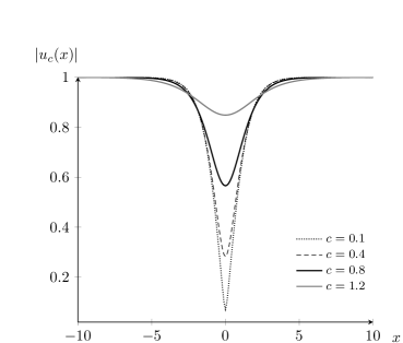
Figure 1: Curve $E_{\textup{min}}$ and solitons in the case $\mathcal{W}=\delta_{0}$.

Since (H1)–(H3) are satisfied by $\mathcal{W}=\delta_{0}$, and since there is uniqueness (up to invariances) of the solutions to (TW${}_{\delta_{0},c}$), we deduce that the branch of solutions given by Theorem 1 corresponds to the dark solitons in (2), for $c\in(0,\sqrt{2})$. In the general case, we do not know if the solution given by Theorem 1 is unique (up to invariances). Actually, the uniqueness for nonlocal equations such as (TW_W,c) can be difficult to establish (see e.g. [3, 46]) and goes beyond the scope of this work. Concerning the regularity, the solutions given by Theorem 1 are smooth and we refer to Lemma 6.2 for a precise statement.

To establish Theorem 1, we analyze two problems. First, we provide some general properties of the curve $E_{\textup{min}}$. Then, we study the compactness of the minimizing sequences associated with $E_{\textup{min}}$. The next result summarizes the properties of $E_{\textup{min}}$.

Theorem 2.

Suppose that $\mathcal{W}$ satisfies (H1) and (H2). Then the following statements hold.

1. The function $E_{\textup{min}}$ is even and Lipschitz continuous on $\mathbb{R}$, with

   $$|E_{\textup{min}}(\mathfrak{p})-E_{\textup{min}}(\mathfrak{q})|\leq\sqrt{2}|\mathfrak{p}-\mathfrak{q}|,\quad\text{ for all }\mathfrak{p},\mathfrak{q}\in\mathbb{R}.$$

   Moreover, it is nondecreasing and subadditive on $\mathbb{R}^{+}$.

2. There exist constants $\mathfrak{q}_{1},A_{1},A_{2},A_{3}>0$ such that

   $$\sqrt{2}\mathfrak{q}-A_{1}\mathfrak{q}^{3/2}\leq E_{\textup{min}}(\mathfrak{q})\leq\sqrt{2}\mathfrak{q}-A_{2}\mathfrak{q}^{5/3}+A_{3}\mathfrak{q}^{2},\quad\text{for all }\mathfrak{q}\in[0,\mathfrak{q}_{1}].$$

3. If (H3) or (H3’) is satisfied, then $E_{\textup{min}}$ is concave on $\mathbb{R}^{+}$.

4. We have $\mathfrak{q}_{*}>0.027$. If $E_{\textup{min}}$ is concave on $\mathbb{R}^{+}$, then $E_{\textup{min}}$ is strictly increasing on $[0,\mathfrak{q}_{*})$, and for all $v\in\mathcal{E}(\mathbb{R})$ satisfying $E(v)<E_{\textup{min}}(\mathfrak{q}_{*})$, we have $v\in\mathcal{N}\mathcal{E}(\mathbb{R})$.

5. Assume that $E_{\textup{min}}$ is concave on $\mathbb{R}^{+}$. Then $E_{\textup{min}}(\mathfrak{q})<\sqrt{2}\mathfrak{q}$, for all $\mathfrak{q}>0$, $E_{\textup{min}}$ is strictly subadditive on $\mathbb{R}^{+}$, and the right and left derivatives of $E_{\textup{min}}$, denoted by $E^{+}_{\min}$ and $E^{-}_{\min}$ respectively, satisfy

   $$0\leq E^{+}_{\min}(\mathfrak{q})\leq E^{-}_{\min}(\mathfrak{q})<\sqrt{2}.$$ (9)

   Furthermore, $E^{+}_{\min}(\mathfrak{q})\to E^{+}_{\min}(0)=\sqrt{2}$, as $\mathfrak{q}\to 0^{+}$.

To prove the existence of solutions we use a concentration-compactness argument. Applying Theorem 2, we show that the minimum is attained at least for $\mathfrak{q}\in(0,\mathfrak{q}_{*})$, so that the set

$$\mathcal{S}_{\mathfrak{q}}=\{v\in\mathcal{N}\mathcal{E}(\mathbb{R}):E(v)=E_{\textup{min}}(\mathfrak{q})\text{ and }p(v)=\mathfrak{q}\}$$

is nonempty, and thus there are nontrivial solutions to (TW_W,c) (see Theorem 6.3). Hence, we can rely on the Cazenave–Lions [22] argument to show that the solutions are stable. Let us remark that the Cauchy problem for (NGP) was studied in [28]. Precisely, using the distance

$$d_{\mathcal{E}}(v_{1},v_{2})=\lVert v_{1}-v_{2}\rVert_{L^{2}(\mathbb{R})+L^{\infty}(\mathbb{R})}+\lVert v^{\prime}_{1}-v^{\prime}_{2}\rVert_{L^{2}(\mathbb{R})}+\lVert|v_{1}|-|v_{2}|\rVert_{L^{2}(\mathbb{R})},$$

the energy space $\mathcal{E}(\mathbb{R})$ is a complete metric space and for every $\Psi_{0}\in\mathcal{E}(\mathbb{R})$ there is a unique global solution $\Psi\in C(\mathbb{R},\mathcal{E}(\mathbb{R}))$ with initial condition $\Psi_{0}$, provided that $\mathcal{W}\in\mathcal{M}_{3}(\mathbb{R})$ and that $\mathcal{W}\geq 0$ or that $\inf_{\mathbb{R}}\widehat{\mathcal{W}}>0$ (see Theorem 5.1). However, these conditions are not necessarily fulfilled by a distribution satisfying (H1)–(H2). Nevertheless, using the energy estimates in Section 2, we can generalize a result in [28] in the following way.

Theorem 3.

Assume that $\mathcal{W}\in\mathcal{M}_{3}(\mathbb{R})$ is an even distribution, with $\widehat{\mathcal{W}}\geq 0$ a.e. on $\mathbb{R}$, and that $\widehat{\mathcal{W}}$ of class $C^{2}$ in a neighborhood of the origin with $\widehat{\mathcal{W}}(0)=1$. Then for every $\Psi_{0}\in\mathcal{E}(\mathbb{R}),$ there exists a unique $\Psi\in C(\mathbb{R},\mathcal{E}(\mathbb{R}))$ global solution to (NGP) with the initial condition $\Psi_{0}$. Moreover, the energy is conserved, as well as the momentum as long as $\inf_{x\in\mathbb{R}}|\Psi(x,t)|>0$.

Remark 1.1.

As explained before, the condition $\widehat{\mathcal{W}}(0)=1$ in Theorem 3 is due to the normalization, and it can be replaced by $\widehat{\mathcal{W}}(0)>0$.

We can also endow $\mathcal{E}(\mathbb{R})$ with the pseudometric distance

$$d(v_{1},v_{2})=\lVert v^{\prime}_{1}-v^{\prime}_{2}\rVert_{L^{2}(\mathbb{R})}+\lVert|v_{1}|-|v_{2}|\rVert_{L^{2}(\mathbb{R})},$$

or with the distance used in [10]

$$d_{A}(v_{1},v_{2})=\lVert v^{\prime}_{1}-v^{\prime}_{2}\rVert_{L^{2}(\mathbb{R})}+\lVert|v_{1}|-|v_{2}|\rVert_{L^{2}(\mathbb{R})}+\lVert v_{1}-v_{2}\rVert_{L^{\infty}([-A,A])},$$

for $A>0$. Notice that $d(v_{1},v_{2})=0$ if and only if $|v_{1}|=|v_{2}|$ and $v_{1}-v_{2}$ is constant. We say that the set $\mathcal{S}_{\mathfrak{q}}$ is orbitally stable in $(\mathcal{E}(\mathbb{R}),d)$ if for all $\Psi_{0}\in\mathcal{E}(\mathbb{R})$ and for all $\varepsilon>0,$ there exists $\delta>0$ such that if

$$d(\Psi_{0},\mathcal{S}_{\mathfrak{q}})\leq\delta,$$

then the solution $\Psi(t)$ of (NGP) associated with the initial condition $\Psi_{0}$ satisfies

$$\sup_{t\in\mathbb{R}}d(\Psi(t),\mathcal{S}_{\mathfrak{q}})\leq\varepsilon.$$

Similarly, the set $\mathcal{S}_{\mathfrak{q}}$ is orbitally stable in $(\mathcal{E}(\mathbb{R}),d_{A})$ if for all $\Psi_{0}\in\mathcal{E}(\mathbb{R})$ and for all $\varepsilon>0,$ there exists $\delta>0$ such that if $d_{A}(\Psi_{0},\mathcal{S}_{\mathfrak{q}})\leq\delta,$ then $\sup_{t\in\mathbb{R}}\inf_{y\in\mathbb{R}}d_{A}(\Psi(\cdot-y,t),\mathcal{S}_{\mathfrak{q}})\leq\varepsilon.$ Here we need to introduce a translation of the flow, since the $d_{A}$ is not invariant under translations.

Now we can state our main result concerning the existence and stability of traveling waves.

Theorem 4.

Suppose that $\mathcal{W}$ satisfies (H1) and (H2), and that $E_{\textup{min}}$ is concave on $\mathbb{R}^{+}$. Then the set $\mathcal{S}_{\mathfrak{q}}$ is nonempty, for all $\mathfrak{q}\in(0,\mathfrak{q}_{*})$. Moreover, every $u\in\mathcal{S}_{\mathfrak{q}}$ is a solution of (TW_W,c) for some speed $c_{\mathfrak{q}}\in(0,\sqrt{2})$ satisfying

$$E^{+}_{\min}(\mathfrak{q})\leq c_{\mathfrak{q}}\leq E^{-}_{\min}(\mathfrak{q}).$$ (10)

Also, $c_{\mathfrak{q}}\to\sqrt{2}$ as $\mathfrak{q}\to 0^{+}$.

In addition, if $\mathcal{W}\in\mathcal{M}_{3}(\mathbb{R})$, then $\mathcal{S}_{\mathfrak{q}}$ is orbitally stable in $(\mathcal{E}(\mathbb{R}),d)$ and in $(\mathcal{E}(\mathbb{R}),d_{A})$, for all $\mathfrak{q}\in(0,\mathfrak{q}_{*})$. Furthermore, for all $\Psi_{0}\in\mathcal{E}(\mathbb{R})$ and for all $\varepsilon>0,$ there exists $\delta>0$ such that if $d(\Psi_{0},\mathcal{S}_{\mathfrak{q}})\leq\delta,$ then the solution $\Psi(t)$ of (NGP) associated with the initial condition $\Psi_{0}$ satisfies

$$\sup_{t\in\mathbb{R}}\inf_{y\in\mathbb{R}}d_{A}(\Psi(\cdot-y,t),\mathcal{S}_{\mathfrak{q}})\leq\varepsilon.$$

In this manner, it is clear that Theorem 1 is an immediate corollary of Theorems 2 and 4, and that the branch of solutions given by Theorem 1 is orbitally stable provided that $\mathcal{W}\in\mathcal{M}_{3}(\mathbb{R})$. In particular, we recover the orbital stability proved by several authors for the solitons given in (2) (see e.g. [47, 16, 24] and the references therein).

We point out that we have not discussed what happens with the minimizing curve for $\mathfrak{q}\geq\mathfrak{q}_{*}$. As mentioned before, for all $\mathfrak{q}>\mathfrak{q}_{*}$, the curve $E_{\textup{min}}(\mathfrak{q})$ is constant for $\mathcal{W}=\delta_{0}$ (see Figure 1) and $\mathcal{S}_{q}$ is empty. Moreover, the critical case $\mathfrak{q}=\mathfrak{q}_{*}$ is associated with the black soliton and its analysis is more involved (see e.g. [12, 39]). Numerical simulations lead us to conjecture that similar results hold for a potential satisfying (H1)-(H3), i.e. that $E_{\textup{min}}(\mathfrak{q})$ is constant and that $\mathcal{S}_{q}$ is empty on $(\mathfrak{q}_{*},\infty)$, and that there is a black soliton when $\mathfrak{q}=\mathfrak{q}_{*}$. In addition, in the performed simulations the value $\mathfrak{q}_{*}$ is close to $\pi/2$ (see Section 7). Furthermore, these simulations also show that (H2) and (H3’) are not necessary for the concavity of $E_{\textup{min}}$ nor the existence of solutions of (TW_W,c). We think that (H2) could be relaxed, but that the condition $(\widehat{\mathcal{W}})^{\prime\prime}(0)>-1$ is necessary. As seen from Theorem 2, we have only used (H3’) as a sufficient condition to ensure the concavity of $E_{\textup{min}}$. If for some $\mathcal{W}$ satisfying (H1) and (H2), one is capable of showing that $E_{\textup{min}}$ is concave, then the existence and stability of solutions of (TW_W,c) is a consequence of Theorem 4.

In addition to the smoothness of the obtained solutions (see Lemma 6.2), it is possible to study further properties of these solitons such as their decay at infinity and uniqueness (up to invariances). Another related open problem is to show the nonexistence of traveling waves for $c>\sqrt{2}$. We will study these questions in a forthcoming paper.

We give now some examples of potentials satisfying conditions (H1), (H2) and (H3)

1. For $\beta>2\alpha>0$, we consider $\mathcal{W}_{\alpha,\beta}=\frac{\beta}{\beta-2\alpha}(\delta_{0}-\alpha e^{-\beta|x|})$, so its Fourier transform is

   $$\widehat{\mathcal{W}}_{\alpha,\beta}(\xi)=\frac{\beta}{\beta-2\alpha}\Big{(}1-\frac{2\alpha\beta}{\xi^{2}+\beta^{2}}\Big{)},$$

   so that $\widehat{\mathcal{W}}_{\alpha,\beta}(0)=1$, and it is simple to check that (H1) and (H2) are satisfied. To verify (H3), it is enough to notice that the only singularity on $\mathbb{H}$ of the meromorphic function $\widehat{\mathcal{W}}_{\alpha,\beta}$ is the simple pole $\nu_{1}=i\beta$ and that

   $$i\operatorname{{\rm Res}}(\widehat{\mathcal{W}}_{\alpha,\beta},i\beta)=-\frac{\alpha\beta}{\beta-2\alpha}<0.$$

   Since $\widehat{\mathcal{W}}_{\alpha,\beta}$ is bounded on $\mathbb{H}$ away from the pole, we conclude that (H3) is fulfilled. We recall that, by the Young inequality, $L^{1}(\mathbb{R})$ is a subset of $\mathcal{M}_{3}(\mathbb{R})$. Therefore $\mathcal{W}_{\alpha,\beta}\in\mathcal{M}_{3}(\mathbb{R})$ and Theorem 4 applies.

2. For $\alpha\in[0,1)$, we take the potential $\mathcal{W}_{\alpha}=\frac{1}{1-\alpha}(\delta_{0}-\alpha\mathcal{V})$, where

   $$\mathcal{V}(x)=-\frac{3}{\pi}\ln(1-e^{-\pi|x|}),\quad\text{and}\quad\widehat{\mathcal{V}}(\xi)=\frac{3(\xi\coth(\xi)-1)}{\xi^{2}}.$$

   It can be seen that $\widehat{\mathcal{V}}$ is a smooth even positive function on $\mathbb{R}$, decreasing on $\mathbb{R}^{+}$, with $\widehat{\mathcal{V}}(0)=1$ and decaying at infinity as $3/\xi$. Thus the conditions (H1) and (H2) are satisfied. As a function on the complex plane, $\widehat{\mathcal{V}}$ is a meromorphic function whose only singularities on $\mathbb{H}$ are given by the simple poles $\{i\pi\ell\}_{\ell\in\mathbb{N}^{*}}$, and

   $$i\operatorname{{\rm Res}}(\widehat{\mathcal{W}}_{\alpha},i\pi\ell)=i\operatorname{{\rm Res}}(-\widehat{\mathcal{V}},i\pi\ell)=-\frac{3}{\pi\ell}.$$

   To check (H3), we define for $k\geq 2$, the functions $\gamma_{1,k}(t)=(k+1/2)\pi+it$, $t\in\leavevmode\nobreak\ [0,(k+1/2)\pi]$, $\gamma_{2,k}(t)=t+i(k+1/2)\pi$, $t\in\leavevmode\nobreak\ [(k+1/2)\pi,-(k+1/2)\pi]$, and $\gamma_{3,k}(t)=-(k+1/2)\pi+it$, $t\in\leavevmode\nobreak\ [(k+1/2)\pi,0]$, so that the corresponding curve $\Gamma_{k}$ is given by the three sides of a square and $\Gamma_{k}$ does not pass through any poles. Using that for $x,y\in\mathbb{R}$ (see e.g. [2])

   $$|\coth(x+iy)|=\Big{|}\frac{\cosh(2x)+\cos(2y)}{\cosh(2x)-\cos(2y)}\Big{|}^{1/2},$$

   we can obtain a constant $C>0$, independent of $k$, such that $|\widehat{\mathcal{V}}(\gamma_{j,k}(t))|\leq C$, for all $t\in[a_{j,k},b_{j,k}]$, for $j\in\{1,2,3\}$, where $[a_{j,k},b_{j,k}]$ is the domain of definition of $\gamma_{j,k}$. As a conclusion, (H3) is fulfilled. Since $V\in L^{1}(\mathbb{R})$, we conclude that $\mathcal{W}_{\alpha}\in\mathcal{M}_{3}(\mathbb{R})$ and therefore we can apply Theorem 4 to this potential.

3. We can also construct perturbations of previous examples. For instance, using the function $\mathcal{V}$ defined above, we set

   $$\widehat{\mathcal{W}}_{\sigma,m}(\xi)=\frac{2m^{2}\pi^{2}}{m^{2}\pi^{2}+2\sigma}\Big{(}1-\frac{\widehat{\mathcal{V}}(\xi)}{2}+\frac{\sigma}{\xi^{2}+m^{2}\pi^{2}}\Big{)},$$

   for $\sigma\in\mathbb{R}$ and $m\in\mathbb{N}^{*}$, so that the poles on $\mathbb{H}$ are still $i\pi\mathbb{N}^{*}$. It follows that for $\sigma>-\pi^{2}m^{2}/2$, the potential satisfies (H1), and that (H3) holds if $\sigma\leq 3$. We can also check that for $\sigma\in(-\pi^{2}m^{2}/2,3]$, $\widehat{\mathcal{W}}_{\sigma,m}$ satisfies (H2), and therefore Theorem 4 applies.

In Section 7 we perform some numerical simulations to illustrate the shape of the solitons and the minimization curves associated with these and other examples. The rest of the paper is organized as follows: we give some energy estimates in Section 2. In Section 3, we establish the properties of the minimizing curve and the proof of Theorem 2, and in Section 4 we show the compactness of the sequences associated with the minimization problem. The orbital stability of the solutions and Theorem 3 are proved in Section 5. We finally complete the proof of Theorem 4 in Section 6.

2 Some a priori estimates

We start by establishing an $L^{\infty}$-estimate for the functions in the energy space in terms of their energy.

Lemma 2.1.

Assume that $\mathcal{W}\in\mathcal{M}_{2}(\mathbb{R})$ satisfies

$$\widehat{\mathcal{W}}(\xi)\geq(1-\kappa\xi^{2})^{+},\quad\text{a.e.\leavevmode\nobreak\ on }\mathbb{R},$$ (2.1)

for some $\kappa\geq 0$. Let $v\in\mathcal{E}(\mathbb{R})$ and set $\eta:=1-|v|^{2}$. Then

$$\lVert\eta\rVert_{L^{\infty}}^{2}\leq 8\tilde{\kappa}E(v)(1+8\tilde{\kappa}E(v)+2\sqrt{2\tilde{\kappa}E(v)})$$ (2.2)

and

$$\lVert\eta\rVert_{L^{2}}^{2}\leq 8\tilde{\kappa}E(v)(1+8\tilde{\kappa}E(v)+2\sqrt{2\tilde{\kappa}E(v)}),$$ (2.3)

with $\tilde{\kappa}=\kappa+1$.

Proof.

Let $\mathcal{W}\in\mathcal{M}_{2}(\mathbb{R})$ and $v\in\mathcal{E}(\mathbb{R})$, and set $\rho=|v|$, $\eta=1-\rho^{2}$ and $x\in\mathbb{R}$. By Plancherel’s identity

$$\eta^{2}(x)=2\int_{-\infty}^{x}\eta\eta^{\prime}\leq\int_{\mathbb{R}}(\eta^{2}+\eta^{\prime 2})=\frac{1}{2\pi}\int_{\mathbb{R}}(1+\xi^{2})|\hat{\eta}|^{2}d\xi.$$ (2.4)

By (2.1), we have $1\leq\widehat{\mathcal{W}}(\xi)+\kappa\xi^{2}$ a.e. on $\mathbb{R}$, so that the term on the right-hand side of (2.4) can be bounded by

$$\frac{1}{2\pi}\int_{\mathbb{R}}(1+\xi^{2})|\hat{\eta}|^{2}\leq\frac{1}{2\pi}\int_{\mathbb{R}}(\widehat{\mathcal{W}}(\xi)+\tilde{\kappa}\xi^{2})|\hat{\eta}|^{2}=4E_{\textup{p}}(v)+\tilde{\kappa}\int_{\mathbb{R}}\eta^{\prime 2},$$ (2.5)

with $\tilde{\kappa}=\kappa+1$. Now we notice that $\eta^{\prime}=-2\rho\rho^{\prime}$, so that $\eta^{\prime 2}\leq 4\lVert v\rVert_{L^{\infty}}^{2}\rho^{\prime 2}$. Also, if $|v|\neq 0$ in some open set, then we can write $v=\rho e^{i\theta}$ and $|v^{\prime}|^{2}=\rho^{\prime 2}+\rho^{2}\theta^{\prime 2}$. On the other hand, the set $\tilde{\Omega}:=\{v=0\}$ coincides with the set $\{\eta=1\}$, and $v^{\prime}=0$ and $\eta^{\prime}=0$ a.e. on $\tilde{\Omega}$. Therefore, we conclude that

$$\eta^{\prime 2}\leq 4\lVert v\rVert_{L^{\infty}}^{2}|v^{\prime}|^{2}\quad\text{ a.e.\leavevmode\nobreak\ on }\mathbb{R}.$$ (2.6)

Combining (2.4), (2.5) and (2.6), we have

$$\eta^{2}(x)\leq 4E_{\textup{p}}(v)+8\tilde{\kappa}\lVert v\rVert_{L^{\infty}}^{2}E_{\textup{k}}(v)\leq\max(4,8\tilde{\kappa}\lVert v\rVert_{L^{\infty}}^{2})E(v).$$ (2.7)

If $\lVert v\rVert^{2}_{L^{\infty}}\leq 1$, inequality (2.2) follows, since $\max(4,8\tilde{\kappa})=8\tilde{\kappa}$. Thus we suppose now that

$$\lVert v\rVert^{2}_{L^{\infty}}>1.$$ (2.8)

Bearing in mind that $\eta(\pm\infty)=0$, we deduce that there is some $x_{0}\in\mathbb{R}$ such that

$$a:=\min_{\mathbb{R}}\eta=\eta(x_{0})=1-\lVert v\rVert^{2}_{L^{\infty}}.$$

Therefore, using (2.7) for $x_{0}$ and (2.8), we get

$$a^{2}\leq 8\tilde{\kappa}(1-a)E(v).$$

Solving the associated quadratic equation and using that $\sqrt{a+b}\leq\sqrt{a}+\sqrt{b}$, we conclude that

$$a\geq\frac{1}{2}(-8\tilde{\kappa}E(v)-\sqrt{64\tilde{\kappa}^{2}E(v)^{2}+32\tilde{\kappa}E(v)})\geq-8\tilde{\kappa}E(v)-2\sqrt{2\tilde{\kappa}E(v)},$$

which implies that

$$\lVert v\rVert^{2}_{L^{\infty}}\leq 1+8\tilde{\kappa}E(v)+2\sqrt{2\tilde{\kappa}E(v)}.$$ (2.9)

By putting together (2.7), (2.8) and (2.9), we obtain (2.2).

To prove (2.3), we use the Plancherel identity and argue as before to get

$$\int_{\mathbb{R}}\eta^{2}\leq\frac{1}{2\pi}\int_{\mathbb{R}}(\widehat{\mathcal{W}}(\xi)+\kappa\xi^{2})|\hat{\eta}|^{2}\leq 4E_{\textup{p}}(v)+\kappa\int_{\mathbb{R}}\eta^{\prime 2}\leq 4E_{\textup{p}}(v)+8\kappa\lVert v\rVert_{L^{\infty}}^{2}E_{\textup{k}}(v).$$

Therefore, using (2.9), inequality (2.3) is established. ∎

Remark 2.2.

Let us suppose that $\mathcal{W}\in\mathcal{M}_{2}(\mathbb{R})$ is even and that also $\widehat{\mathcal{W}}$ is of class $C^{2}$ in some interval $[-r,r]$, with $r>0$. Then $(\widehat{\mathcal{W}})^{\prime}(0)=0$, and by the Taylor theorem we deduce that for any $\xi\in(-r,r)$, there exists $\tilde{\xi}\in(-r,r)$ such that

$$\widehat{\mathcal{W}}(\xi)=1+(\widehat{\mathcal{W}})^{\prime\prime}(\tilde{\xi})\frac{\xi^{2}}{2}\geq 1-\mu\xi^{2},$$

where $\mu=\max_{[-r,r]}|(\widehat{\mathcal{W}})^{\prime\prime}|/2$. If $1/\mu\leq r^{2}$, we set $\kappa=\mu$. If $1/\mu>r^{2}$, we take $\kappa=1/r^{2}$. Assuming also that $\widehat{\mathcal{W}}\geq 0$ a.e. on $\mathbb{R}$, we conclude that in both cases condition (2.1) is fulfilled.

From now on until the end of this paper, we assume that (H1) and (H2) are satisfied, so in particular Lemma 2.1 holds true with $\kappa=1/2$. In the sequel, we also use the identity

$$\int_{\mathbb{R}}(\mathcal{W}*f)g=\int_{\mathbb{R}}(\mathcal{W}*g)f,\quad\text{ for all }f,g\in L^{2}(\mathbb{R}),$$ (2.10)

that is a consequence of parity of $\mathcal{W}$ stated in (H1).

A key point to obtain the compactness of the sequences in Section 4 is that the momentum can be controlled by the energy. This kind of inequality is crucial in the arguments when proving the existence of solitons by variational techniques in the case $\mathcal{W}=\delta_{0}$ (see [11, 25]). Moreover, for an open set $\Omega\subset\mathbb{R}$ and $u={\rho}e^{i\theta}\in\mathcal{N}\mathcal{E}(\mathbb{R})$, we need to be able to control the localized momentum

$$p_{\Omega}(u):=\frac{1}{2}\int_{\Omega}\eta\theta^{\prime},$$

by some localized version of the energy. By the Cauchy inequality, setting as usual $\eta=1-|u|^{2}$, we have

$$\sqrt{2}|p_{\Omega}(u)| \leq\ \frac{1}{4}\int_{\Omega}\eta^{2}+\frac{1}{2}\int_{\Omega}\theta^{\prime 2}\leq\frac{1}{4}\int_{\Omega}\eta^{2}+\frac{1}{2\underset{\Omega}{\inf}{\rho}^{2}}\int_{\Omega}\rho^{2}\theta^{\prime 2},$$ (2.11)

but it is not clear how to define a localized version of energy, due the to the nonlocal interactions. We propose to introduce the localized energy

$$E_{\Omega}(u):=\frac{1}{2}\int_{\Omega}|u^{\prime}|^{2}+\frac{1}{4}\int_{\Omega}(\mathcal{W}\ast{\eta_{\Omega}}){\eta_{\Omega}},\quad\text{ with }\eta_{\Omega}:=\eta\mathds{1}_{\Omega}.$$

Notice that if $\Omega=\mathbb{R}$, then $E_{\Omega}(u)=E(u)$ and $p_{\Omega}(u)=p(u)$. Since $\eta_{\Omega}$ can be discontinuous (and thus not weakly differentiable) when $\Omega$ is bounded, we also need to introduce a smooth cut-off function as follows: for $\Omega_{0}$ an open set compactly contained in $\Omega$, i.e. $\Omega_{0}\subset\subset\Omega$, we set a function $\chi_{\Omega,\Omega_{0}}\in C^{\infty}(\mathbb{R})$ taking values in $[0,1]$ and satisfying

$$\chi_{\Omega,\Omega_{0}}(x)=\begin{cases}1&\text{ if }x\in\Omega_{0},\\ 0&\text{ if }x\in\mathbb{R}\setminus\Omega.\end{cases}$$ (2.12)

In the case $\Omega=\Omega_{0}=\mathbb{R}$, we simply set $\chi_{\Omega,\Omega_{0}}\equiv 1$.

Lemma 2.3.

Let $\Omega,\Omega_{0}\subset\mathbb{R}$ be two smooth open sets with $\Omega_{0}\subset\subset\Omega$ and let $\chi_{\Omega,\Omega_{0}}\in C^{\infty}(\mathbb{R})$ as above. Let $u\in\mathcal{E}(\mathbb{R})$ and assume that there is some $\varepsilon\in(0,1)$ such that $1-\varepsilon\leq|u|^{2}\leq 1+\varepsilon$ on $\Omega$. Then

$$\sqrt{2}|p_{\Omega}(u)|\leq\frac{E_{\Omega}(u)}{1-\varepsilon}+\Delta_{\Omega}(u),$$ (2.13)

where the remainder term $\Delta_{\Omega}(u)$ satisfies the estimate

$$|\Delta_{\Omega}(u)|\leq C(\|\eta\|_{L^{2}(\Omega\setminus\Omega_{0})}+\|\eta\chi_{\Omega,\Omega_{0}}^{\prime}\|_{L^{2}(\Omega\setminus\Omega_{0})}+\|\eta\chi_{\Omega,\Omega_{0}}^{\prime}\|_{L^{2}(\Omega\setminus\Omega_{0})}^{2}).$$ (2.14)

Here $C=C(E(u),\varepsilon)$ is a constant depending on $E(u)$ and $\varepsilon$, but not on $\Omega$ nor $\Omega_{0}$. In particular, in the case $\Omega=\Omega_{0}=\mathbb{R},$ we have

$$|p(u)|\leq\frac{E(u)}{\sqrt{2}(1-\varepsilon)}.$$ (2.15)

Proof.

As usual, we write $u=\rho e^{i\theta}$ on $\Omega$. As in (2.11), using the Cauchy inequality and that $1-\varepsilon\leq\rho^{2}\leq 1+\varepsilon_{2}$ on $\Omega$, we have

$$\sqrt{2}|p_{\Omega}(u)|\leq\frac{\sigma}{4}\int_{\Omega}\eta^{2}+\frac{1}{2\sigma(1-\varepsilon)}\int_{\Omega}\rho^{2}\theta^{\prime 2},$$ (2.16)

with $\sigma>0$ to be fixed later. Now, we write

$$\frac{\sigma}{4}\int_{\Omega}\eta^{2}+\frac{1}{2\sigma(1-\varepsilon)}\int_{\Omega}\rho^{2}\theta^{\prime 2}=\frac{\sigma}{4}\int_{\Omega}\Big{(}\eta_{\Omega}^{2}-{(\mathcal{W}\ast\eta_{\Omega})\eta_{\Omega}}\Big{)}+{R_{\Omega}(u)},$$

where

$$R_{\Omega}(u):=\frac{\sigma}{4}\int_{\Omega}(\mathcal{W}\ast\eta_{\Omega})\eta_{\Omega}+\frac{1}{2\sigma(1-\varepsilon)}\int_{\Omega}\rho^{2}\theta^{\prime 2}.$$

Let $\tilde{\eta}_{\Omega}=\eta\chi_{\Omega,\Omega_{0}}$ and

$$\Delta_{1,\Omega}(u):=\frac{\sigma}{4}\int_{\mathbb{R}}\Big{(}\big{(}\eta_{\Omega}^{2}-\tilde{\eta}_{\Omega}^{2}\big{)}-(\mathcal{W}\ast\eta_{\Omega})\eta_{\Omega}+(\mathcal{W}\ast\tilde{\eta}_{\Omega})\tilde{\eta}_{\Omega}\Big{)}.$$ (2.17)

Using the Plancherel theorem and (H2), we have

$$\frac{\sigma}{4}\int_{\Omega}\Big{(}\eta_{\Omega}^{2}-(\mathcal{W}\ast\eta_{\Omega})\eta_{\Omega}\Big{)} =\frac{\sigma}{4}\int_{\mathbb{R}}\Big{(}\tilde{\eta}_{\Omega}^{2}-(\mathcal{W}\ast\tilde{\eta}_{\Omega})\tilde{\eta}_{\Omega}\Big{)}+\Delta_{1,\Omega}(u)$$

$$=\frac{\sigma}{8\pi}\int_{\mathbb{R}}|\widehat{\tilde{\eta}_{\Omega}}|^{2}\Big{(}1-\widehat{\mathcal{W}}(\xi)\Big{)}+\Delta_{1,\Omega}(u)$$

$$\leq\frac{\sigma}{16\pi}\int_{\mathbb{R}}\xi^{2}|\widehat{\tilde{\eta}_{\Omega}}|^{2}+\Delta_{1,\Omega}(u)$$

$$=\frac{\sigma}{8}\int_{\mathbb{R}}({\tilde{\eta}_{\Omega}}^{\prime})^{2}+\Delta_{1,\Omega}(u).$$

Noticing that

$$\tilde{\eta}_{\Omega}^{\prime 2}=({\eta}^{\prime}\chi_{\Omega,\Omega_{0}})^{2}+2\eta{\eta}^{\prime}\chi_{\Omega,\Omega_{0}}\chi_{\Omega,\Omega_{0}}^{\prime}+({\eta}\chi_{\Omega,\Omega_{0}}^{\prime})^{2},$$

and that $0\leq\chi_{\Omega,\Omega_{0}}\leq 1$, by putting together the estimates above, we conclude that

$$\sqrt{2}|p_{\Omega}(u)|\leq\frac{\sigma}{8}\int_{\Omega}\eta^{\prime 2}+{R_{\Omega}(u)}+\Delta_{\Omega}(u),$$

where the remainder term is given by

$$\Delta_{\Omega}(u)=\Delta_{1,\Omega}(u)+\Delta_{2,\Omega}(u),\quad\Delta_{2,\Omega}(u):=\frac{\sigma}{8}\int_{\Omega}\big{(}2\eta{\eta}^{\prime}\chi_{\Omega,\Omega_{0}}\chi_{\Omega,\Omega_{0}}^{\prime}+({\eta}\chi_{\Omega,\Omega_{0}}^{\prime})^{2}\big{)}.$$

Therefore, since $\eta^{\prime 2}\leq 4(1+\varepsilon)\rho^{\prime 2}$, taking $\sigma=1/\sqrt{1-\varepsilon^{2}}$, we obtain

$$\sqrt{2}|p_{\Omega}(u)|\leq\frac{\sqrt{1-\varepsilon^{2}}}{1-\varepsilon}\int_{\Omega}\Big{(}\frac{\rho^{\prime 2}}{2}+\frac{\rho^{2}\theta^{\prime 2}}{2}\Big{)}+\frac{1}{4\sqrt{1-\varepsilon^{2}}}\int_{\Omega}(\mathcal{W}\ast\eta_{\Omega})\eta_{\Omega}+\Delta_{\Omega}(u),$$

which gives us (2.13). It remains to show the estimate in (2.14). For the first term in $\Delta_{1,\Omega}$, we see that

$$\int_{\Omega}\left|\eta_{\Omega}^{2}-\tilde{\eta}_{\Omega}^{2}\right|=\int_{\Omega\setminus\Omega_{0}}\eta^{2}\left|\mathds{1}_{\Omega}^{2}-\chi_{\Omega,\Omega_{0}}^{2}\right|\leq\|\eta\|_{L^{2}(\Omega\setminus\Omega_{0})}^{2}.$$ (2.18)

For the other term in $\Delta_{1,\Omega}$, using (2.10), we have

$$\left|\int_{\mathbb{R}}(\mathcal{W}\ast\eta_{\Omega})\eta_{\Omega}-(\mathcal{W}\ast\tilde{\eta}_{\Omega})\tilde{\eta}_{\Omega}\right| =\left|\int_{\mathbb{R}}(\mathcal{W}\ast(\eta_{\Omega}+\tilde{\eta}_{\Omega}))(\eta_{\Omega}-\tilde{\eta}_{\Omega})\right|$$

$$\leq 4\|\mathcal{W}\|_{\mathcal{M}_{2}}\|\eta\|_{L^{2}(\mathbb{R})}\|\eta\|_{L^{2}(\Omega\setminus\Omega_{0})}.$$ (2.19)

Concerning in $\Delta_{2,\Omega}$, we have

$$|\Delta_{2,\Omega}|\leq\frac{\sigma}{8}\big{(}4\|u\|_{L^{\infty}(\mathbb{R})}\|u^{\prime}\|_{L^{2}(\mathbb{R})}\|\eta\chi_{\Omega,\Omega_{0}}^{\prime}\|_{L^{2}(\Omega\setminus\Omega_{0})}+\|\eta\chi_{\Omega,\Omega_{0}}^{\prime}\|_{L^{2}(\Omega\setminus\Omega_{0})}^{2}\big{)}.$$ (2.20)

By putting together (2.18), (2.19) and (2.20), and invoking Lemma 2.1, we obtain (2.14). ∎

From now on, we set for $\mathfrak{q}>0,$

$$\Sigma_{\mathfrak{q}}:=1-\frac{E_{\min}(\mathfrak{q})}{\sqrt{2}\mathfrak{q}}.$$ (2.21)

In this manner, the condition $E_{\min}(\mathfrak{q})<\sqrt{2}\mathfrak{q}$ is equivalent to $\Sigma_{\mathfrak{q}}>0$. We also define for $\mathfrak{q}>0$ and $\delta>0$, the set

$$X_{\mathfrak{q},\delta}:=\{v\in\mathcal{N}\mathcal{E}(\mathbb{R}):|p(v)-\mathfrak{q}|\leq\delta\leavevmode\nobreak\ \textup{and}\leavevmode\nobreak\ |E(v)-E_{\min}(\mathfrak{q})|\leq\delta\}.$$ (2.22)

Lemma 2.4.

Let $\mathfrak{q}>0$, $L>1$ and suppose that $\Sigma_{\mathfrak{q}}>0$. Then there is $\delta_{0}>0$ such that for all $\delta\in[0,\delta_{0}]$ and for all $v\in X_{q,\delta}$, there exists $\bar{x}\in\mathbb{R}$ such that

$$\left|1-|v(\bar{x})|^{2}\right|\geq\frac{\Sigma_{\mathfrak{q}}}{L}.$$

Proof.

We argue by contradiction and suppose that the statement is false. Hence, for all $\delta_{0}>0,$ there exists $\delta\in[0,\delta_{0}]$ and $v\in X_{\mathfrak{q},\delta}$ such that

$$\|1-|v|^{2}\|_{L^{\infty}(\mathbb{R})}<\Sigma_{\mathfrak{q}}/L.$$

Then, taking $\delta_{0}=1/n,$ there is $\delta_{n}\in[0,\frac{1}{n}]$ and $v_{n}\in X_{\mathfrak{q},\delta_{n}}$ such that

$$\|1-|v_{n}|^{2}\|_{L^{\infty}(\mathbb{R})}<\Sigma_{\mathfrak{q}}/L.$$

Since $\Sigma_{\mathfrak{q}}\in(0,1]$, considering $\varepsilon=\Sigma_{\mathfrak{q}}/L$, we have $\varepsilon\in(0,1)$. Therefore we can apply Lemma 2.3 to conclude that

$$\sqrt{2}|p(v_{n})|\leq\frac{1}{(1-{\Sigma_{\mathfrak{q}}}/{L})}E(v_{n}),$$

and letting $n\to\infty$, we get

$${\sqrt{2}\mathfrak{q}\Big{(}1-\frac{\Sigma_{\mathfrak{q}}}{L}\Big{)}}\leq E_{\min}(\mathfrak{q}),$$

which is equivalent to $\Sigma_{\mathfrak{q}}\leq{\Sigma_{\mathfrak{q}}}/{L},$ contradicting the fact that $L>1$. ∎

Lemma 2.5.

Let $E>0$ and $0<m_{0}<1$ be two constants. There is $l_{0}\in\mathbb{N}$, depending on $E$ and $m_{0}$, such that for any function $v\in\mathcal{E}(\mathbb{R})$ satisfying $E(v)\leq E$, one of the following holds:

1. For all $x\in\mathbb{R}$, $|1-|v(x)|^{2}|<m_{0}$.

2. There exist $l$ points $x_{1},x_{2},\dots,x_{l}$, with $l\leq l_{0}$, such that

   $$|1-|v(x_{j})|^{2}|\geq m_{0},\ \forall 1\leq j\leq l,\quad\text{ and }\quad|1-|v(x)|^{2}|\leq m_{0},\ \forall x\in\mathbb{R}\setminus\bigcup_{j=1}^{l}[x_{j}-1,x_{j}+1].$$

Proof.

The proof is a rather standard consequence of the energy estimates. For the sake of completeness, we give a proof similar to the one given in [10].

Let us suppose that (i) does not hold. Then the set

$$\mathcal{C}=\{z\in\mathbb{R}:|\eta(z)|\geq m_{0}\},$$

is nonempty, where $\eta=1-|v|^{2}$ as usual. Setting $I_{j}=[j-1/2,j+1/2]$, for $j\in\mathbb{Z}$, the assertion in (ii) will follow if we show that $l:=\text{Card}\{j\in\mathbb{Z},\leavevmode\nobreak\ I_{j}\cap\mathcal{C}\neq\emptyset\}$ can be bounded by some $l_{0}$, depending only on $E$ and $m_{0}$.

Using that $||v|^{\prime}|=|v^{\prime}|$ (see Lemma 7.6 in [36]), the Cauchy–Schwarz inequality and (2.2), we deduce that there exists a constant $C$, depending on $E$, such that for all $x,y\in\mathbb{R}$,

$$||v(x)|^{2}-|v(y)|^{2}|=2\left|\int_{x}^{y}|v|^{\prime}|v|\right|\leq 2\|v\|_{L^{\infty}(\mathbb{R})}\|v^{\prime}\|_{L^{2}(\mathbb{R})}|x-y|^{\frac{1}{2}}\leq C|x-y|^{1/2}.$$

Thus, setting $r={m_{0}^{2}}/(4C^{2})$, we deduce that for any $z\in\mathcal{C}$ and for any $y\in[z-r,z+r]$,

$$|\eta(y)|\geq m_{0}-||v(y)|^{2}-|v(z)|^{2}|\geq\frac{m_{0}}{2}.$$

Taking $r_{0}=\min(r,1/2)$ and integrating this inequality, we get, for any $z\in\mathcal{C}$,

$$\int_{z-r_{0}}^{z+r_{0}}\eta^{2}(y)dy\geq\frac{{m_{0}^{2}}r_{0}}{4}.$$

Noticing that $[z-r_{0},z+r_{0}]\subset\tilde{I_{j}}:=[j-1,j+1]$, if $z\in I_{j}\cap{\mathcal{C}}$, we conclude that

$$\frac{\tilde{l}{m_{0}^{2}}r_{0}}{4}\leq\sum_{j\in\mathbb{\mathbb{Z}},\tilde{I}_{j}\cap\mathcal{C}\neq\emptyset}\int_{\tilde{I_{j}}}\eta^{2}\leq 2\lVert\eta\rVert_{L^{2}(\mathbb{R})}^{2},$$

where $\tilde{l}:=\text{Card}\{j\in\mathbb{Z}:\tilde{I}_{j}\cap\mathcal{C}\neq\emptyset\}$. The conclusion follows from (2.3), taking $l_{0}=2\tilde{l}$, since $l\leq 2\tilde{l}$. ∎

3 Properties of the minimizing curve

For the study of the minimizing curve, it will be useful to use finite energy smooth functions that are constant far away from the origin. For this purpose we introduce the set

$$\mathcal{E}^{\infty}_{0}(\mathbb{R})=\{v\in\mathcal{N}\mathcal{E}(\mathbb{R})\cap C^{\infty}(\mathbb{R}):\exists R>0\text{ s.t.\ }v\text{ is constant on }B(0,R)^{c}\}.$$

Notice that in the functions in the space $\mathcal{E}^{\infty}_{0}(\mathbb{R})$ can have different values near $+\infty$ and near $-\infty$. Bearing in mind that the solitons $u_{c}$ in (2) satisfy $u_{c}(+\infty)\neq u_{c}(-\infty)$, we will see that these kinds of functions are well-adapted to approximate the solutions of (TW_W,c).

The next result shows that $E_{\textup{min}}$ is well defined and that its graph lies under the line $y=\sqrt{2}x$ on $\mathbb{R}^{+}$.

Lemma 3.1.

For all $\mathfrak{q}\in\mathbb{R}$, there exists a sequence $v_{n}\in\mathcal{E}^{\infty}_{0}(\mathbb{R})$ satisfying

$$p(v_{n})=\mathfrak{q}\quad\text{ and }\quad E(v_{n})\rightarrow\sqrt{2}|\mathfrak{q}|,\quad\text{ as }n\to\infty.$$ (3.1)

In particular the function $E_{\textup{min}}:\mathbb{R}\to\mathbb{R}$ is well defined, and for all $\mathfrak{q}\geq 0$

$$E_{\min}(\mathfrak{q})\leq\sqrt{2}\mathfrak{q}.$$ (3.2)

Proof.

The case $\mathfrak{q}=0$ is trivial since it is enough to take $v\equiv 1$. Let us assume that $\mathfrak{q}>0$ and consider $\chi\in C_{0}^{\infty}(\mathbb{R})$ such that $\int_{\mathbb{R}}\chi^{\prime 2}={\mathfrak{q}}/{\sqrt{2}}$. Let us define

$$a=\frac{\sqrt{2}}{2}\int_{\mathbb{R}}\chi^{\prime}(y)^{3}dy,\quad\alpha_{n}=\frac{1}{n}\quad\text{ and }\quad\beta_{n}=\frac{1}{n^{2}}-\frac{a}{\mathfrak{q}n^{3}}.$$

Then it is enough to consider

$$v_{n}=\rho_{n}e^{i\theta_{n}},\quad\text{ where }\rho_{n}(x)=1-\alpha_{n}\chi^{\prime}(\beta_{n}x)\text{ and }\theta_{n}(x)=\sqrt{2}\frac{\alpha_{n}}{\beta_{n}}\chi(\beta_{n}x).$$

We can assume that $v_{n}$ does not vanish since $|v_{n}|=|\rho_{n}|\geq 1-|\alpha_{n}|\|\chi^{\prime}\|_{L^{\infty}(\mathbb{R})}.$ Thus the momentum of $v_{n}$ is well defined and we have

$$p(v_{n}) =\frac{1}{2}\int_{\mathbb{R}}(1-\rho_{n}^{2})\theta_{n}^{\prime}=\frac{\sqrt{2}}{2\beta_{n}}\int_{\mathbb{R}}(2\alpha_{n}\chi^{\prime}(y)-\alpha_{n}^{2}\chi^{\prime}(y)^{2})\alpha_{n}\chi^{\prime}(y)dy$$

$$=\frac{\alpha_{n}^{2}}{\beta_{n}}\mathfrak{q}-\frac{\alpha_{n}^{3}}{\beta_{n}}a=\mathfrak{q}.$$

It remains to show that $E(v_{n})\to\sqrt{2}\mathfrak{q}$. For the kinetic part, we have

$$E_{\textup{k}}(v_{n}) =\int_{\mathbb{R}}(1-\alpha_{n}\chi^{\prime}(\beta_{n}x))\alpha_{n}\chi^{\prime}(\beta_{n}x)^{2}dx+\frac{1}{2}\int_{\mathbb{R}}(\alpha_{n}\beta_{n}\chi^{\prime\prime}(\beta_{n}x))^{2}dx$$

$$=\frac{\alpha_{n}^{2}}{\beta_{n}}\int_{\mathbb{R}}(1-\alpha_{n}\chi^{\prime}(y))\chi^{\prime}(y)^{2}dy+\frac{\alpha_{n}^{2}\beta_{n}}{2}\int_{\mathbb{R}}\chi^{\prime\prime}(y)^{2}dy$$

$$\to\int_{\mathbb{R}}\chi^{\prime}(y)^{2}dy=\frac{\mathfrak{q}}{\sqrt{2}},$$

since $\alpha_{n},\beta_{n}\to 0$ and $\alpha_{n}^{2}/\beta_{n}\to 1$. For the potential energy, using Plancherel’s theorem, the dominated convergence theorem and the continuity of $\widehat{\mathcal{W}}$ at $0$, we get

$$E_{\textup{p}}(v_{n}) =\frac{1}{8\pi}\int_{\mathbb{R}}\widehat{\mathcal{W}}(\xi)|\mathcal{F}(1-\rho_{n}^{2})|^{2}(\xi)d\xi=\frac{\alpha_{n}^{2}}{8\beta_{n}\pi}\int_{\mathbb{R}}\widehat{\mathcal{W}}(\beta_{n}\xi)|\mathcal{F}(2\chi^{\prime}-\alpha_{n}\chi^{\prime 2})|^{2}\left({\xi}\right)d\xi$$

$$\to\int_{\mathbb{R}}\chi^{\prime 2}(y)dy=\frac{\mathfrak{q}}{\sqrt{2}}.$$

Therefore we conclude that (3.1) holds true for $\mathfrak{q}\geq 0$. In the situation $\mathfrak{q}<0$, it is enough to proceed as above taking

$$\int_{\mathbb{R}}\chi^{\prime 2}=\frac{|\mathfrak{q}|}{\sqrt{2}}=-\frac{{\mathfrak{q}}}{\sqrt{2}}\quad\text{ and}\quad v_{n}=\rho_{n}e^{-i\theta_{n}}.$$

This concludes the proof of (3.1). By the definition of $E_{\textup{min}}$, we also have $E_{\textup{min}}(\mathfrak{q})\leq E(v_{n}).$ Letting $n\to\infty$, we obtain (3.2). ∎

Lemma 3.2.

The curve $E_{\min}$ is even on $\mathbb{R}$.

Proof.

Let $\mathfrak{q}\in\mathbb{R}$ and $u_{n}=\rho_{n}e^{i\phi_{n}}\in\mathcal{N}\mathcal{E}(\mathbb{R})$ be such that $E(u_{n})\to E_{\min}(\mathfrak{q})$ and $p(u_{n})=\mathfrak{q}.$ Setting ${v_{n}}=\rho_{n}e^{-i\phi_{n}}$, it is immediate to verify that $E(v_{n})=E(u_{n})$ and that $p(v_{n})=-p(u_{n})=-\mathfrak{q}$. Therefore

$$E(v_{n})\geq E_{\min}(-\mathfrak{q}),$$

and letting $n\to\infty$ we conclude that $E_{\min}(\mathfrak{q})\geq E_{\min}(-\mathfrak{q}).$ Replacing $\mathfrak{q}$ by $-\mathfrak{q}$, we deduce that $E_{\min}(-\mathfrak{q})=E_{\min}(\mathfrak{q})$, i.e. that $E_{\textup{min}}$ is even. ∎

Corollary 3.3.

The constant defined in (8) satisfies $\mathfrak{q}_{*}>0.027$.

Proof.

Let $v\in\mathcal{E}(\mathbb{R})$, with $E(v)\leq E_{\textup{min}}(\mathfrak{q})$. Then, by combining (2.2) and (3.2), with $\tilde{\kappa}=3/2$, we have

$$\lVert 1-|v|^{2}\rVert_{L^{\infty}}^{2}\leq 12\sqrt{2}\mathfrak{q}(1+12\sqrt{2}\mathfrak{q}+2(3\sqrt{2}\mathfrak{q})^{\frac{1}{2}}).$$

Since the right-hand is an increasing function of $\mathfrak{q}$, and since the solution of the equation $12\sqrt{2}z(1+12\sqrt{2}z+2(3\sqrt{2}z)^{\frac{1}{2}})=1$ is

$$z=\frac{\sqrt{2}}{288}\frac{\big{(}(12\sqrt{3}+4\sqrt{31})^{2/3}-4\big{)}^{2}}{(12\sqrt{3}+4\sqrt{31})^{2/3}}\approx 0.0274,$$

the conclusion follows from the definition of $\mathfrak{q}_{*}$. ∎

In view of Lemma 3.2, it is enough to study $E_{\textup{min}}$ on $\mathbb{R}^{+}$. Concerning the density of the space $\mathcal{E}_{0}^{\infty}(\mathbb{R})$ in $\mathcal{N}\mathcal{E}(\mathbb{R})$, we have the following result.

Lemma 3.4.

Let $v=\rho e^{i\theta}\in\mathcal{N}\mathcal{E}(\mathbb{R})$. Then there exists a sequence functions $v_{n}=\rho_{n}e^{i\theta}$ in $\mathcal{E}^{\infty}_{0}(\mathbb{R})$, with $\rho_{n}-1,\theta_{n}^{\prime}\in C_{c}^{\infty}(\mathbb{R})$, such that

$$\lVert\rho_{n}-\rho\rVert_{H^{1}(\mathbb{R})}+\lVert\theta^{\prime}_{n}-\theta^{\prime}\rVert_{L^{2}(\mathbb{R})}\to 0,\quad\text{ as }n\to\infty.$$ (3.3)

In particular

$$E(v_{n})\to E(v)\quad\text{ and }\quad p(v_{n})\to p(v),\quad\text{ as }n\to\infty.$$ (3.4)

Proof.

Since $v=\rho e^{i\theta}\in\mathcal{N}\mathcal{E}(\mathbb{R})$, we deduce that $v\in L^{\infty}(\mathbb{R})$ and that $|v(x)|\to 1$, as $|x|\to\infty$. Let

$$g(x):=\rho(x)-1=|v(x)|-1=\frac{|v(x)|^{2}-1}{|v(x)|+1}.$$

Then $g\in L^{2}(\mathbb{R})$ and since $g^{\prime}=\langle v^{\prime},v\rangle/|v|$, we conclude that $g\in H^{1}(\mathbb{R})$. Therefore, there exists $g_{n}\in C_{c}^{\infty}(\mathbb{R})$ such that $g_{n}\to g$ in $H^{1}(\mathbb{R})$. Setting $\rho_{n}=g_{n}+1$, we deduce that $\lVert\rho_{n}-\rho\rVert_{H^{1}}\to 0$, as $n\to\infty.$

Concerning $\theta$, using the density of $C_{c}^{\infty}(\mathbb{R})$ in $L^{2}(\mathbb{R})$, we get the existence of a sequence $\phi_{n}\in C_{c}^{\infty}(\mathbb{R})$ converging to $\theta^{\prime}$ in $L^{2}(\mathbb{R})$. Hence, taking

$$\theta_{n}(x)=\int_{-\infty}^{x}\phi_{n},$$ (3.5)

we conclude that $\theta_{n}^{\prime}-\theta^{\prime}\to 0$ in $L^{2}(\mathbb{R})$ and that $v_{n}:=\rho_{n}e^{i\theta_{n}}$ belongs to $\mathcal{E}^{\infty}_{0}(\mathbb{R})$. The convergences in (3.4) are a direct consequence of the convergences in (3.3) and the Sobolev injection $H^{1}(\mathbb{R})\hookrightarrow L^{\infty}(\mathbb{R})$. ∎

Remark 3.5.

If $v\in\mathcal{E}^{\infty}_{0}(\mathbb{R})$, then we can write $v=\rho e^{i\theta}$, with $\rho,\theta\in C^{\infty}(\mathbb{R})$ and such that $\rho-1,\theta^{\prime}\in C_{c}^{\infty}(\mathbb{R})$. Hence the function $\theta$ is constant outside $\operatorname{{\rm supp}}(\theta^{\prime})$ and without loss of generality we can assume that there is $R>0$ such that $\theta(x)\equiv 0$ for all $x\leq-R$, or that $\theta(x)\equiv 0$ for all $x\geq R$ (but we cannot assume that $\theta(x)\equiv 0$ for all $|x|\geq R$). Therefore, w.l.o.g.  we can suppose that $v(x)\equiv 1$ for all $x\leq-R$ or that $v(x)\equiv 1$ for all $x\geq R$, for some $R>0$ large enough.

To handle the nonlocal interaction term in the energy in the construction of comparison sequences, we use introduce the functional

$$B(f):=\int_{\mathbb{R}}(\mathcal{W}*f)f,$$

for $f\in L^{2}(\mathbb{R};\mathbb{R}).$ It is clear that if $u\in\mathcal{E}(\mathbb{R})$, then $B(1-|u|^{2})=4E_{\textup{p}}(u).$ The following elementary lemma will be useful.

Lemma 3.6.

For all $f,g\in L^{2}(\mathbb{R})$ we have

$$B(f+g)=B(f)+B(g)+2\int_{\mathbb{R}}(\mathcal{W}*f)g.$$ (3.6)

Assume further that $g\in C_{c}^{\infty}(\mathbb{R})$ and that there is a sequence of numbers $(y_{n})$ such that $y_{n}\to\infty$, as $n\to\infty$. Then, setting set $g_{n}(x)=g(x-y_{n})$, we have

$$B(f+g_{n})-B(f)-B(g_{n})=2\int_{\mathbb{R}}(\mathcal{W}*f)g_{n}\to 0,\quad\text{ as }n\to\infty.$$ (3.7)

Proof.

The identity (3.6) is a direct consequence of (2.10). The convergence in (3.7) follows from the fact that $g_{n}\rightharpoonup 0$ in $L^{2}(\mathbb{R})$. ∎

We finally conclude that we can modify a function with energy close to $E_{\textup{min}}(\mathfrak{q})$ such that it is constant far away, but the momentum remains unchanged.

Corollary 3.7.

Let $u=\rho e^{i\theta}\in\mathcal{N}\mathcal{E}(\mathbb{R})$. There exists a sequence $u_{n}\in\mathcal{E}^{\infty}_{0}(\mathbb{R})$ such that

$$p(u_{n})=p(u)\quad\text{ and }\quad E(u_{n})\to E(u),\quad\text{ as }n\to\infty.$$ (3.8)

Proof.

Let $v_{n}=\rho_{n}e^{i\theta}\in\mathcal{E}^{\infty}_{0}(\mathbb{R})$ be the sequence given by Lemma 3.4 such that

$$E(v_{n})\to E(u)\quad\text{ and }\quad p(v_{n})\to p(u),\quad\text{ as }n\to\infty.$$ (3.9)

If $p(u)\neq 0$, we set $\alpha_{n}=p(u)/p(v_{n})$. Therefore $\alpha_{n}\to 1$ and it is straightforward to verify that the sequence $u_{n}=\rho_{n}e^{i\alpha_{n}\theta_{n}}$ satisfies (3.8).

The case $p(u)=0$ is more involved. In this instance, we may assume that $\delta_{n}:=p(v_{n})\neq 0$ for $n$ sufficiently large. Otherwise, up to a subsequence, the conclusion holds with $u_{n}=v_{n}$. By Lemma 3.1, we get the existence of a sequence $w_{n}\in\mathcal{E}_{0}^{\infty}(\mathbb{R})$ such that

$$p(w_{n})=-\delta_{n}\quad\text{ and }\quad E(w_{n})\rightarrow 0,\quad\text{ as }n\to\infty.$$ (3.10)

Let $R_{n},r_{n}>0$ be such that the functions

$$f_{n}:=1-|v_{n}|^{2}\quad\text{ and }\quad g_{n}:=1-|w_{n}|^{2}$$

are supported in the balls $B(0,R_{n})$ and $B(0,r_{n})$, respectively. Taking into account Remark 3.5, without loss of generality, we can assume that the following function is continuous and belongs to $\mathcal{E}^{\infty}_{0}(\mathbb{R})$

$$u_{n}=\begin{cases}v_{n},&\text{ on }\ (-\infty,R_{n}),\\ 1,&\text{ on }[R_{n},-r_{n}+y_{n}],\\ w_{n}(\cdot-y_{n}),&\text{ on }(-r_{n}+y_{n},\infty),\end{cases}$$ (3.11)

where $y_{n}$ is a sequence of points such that $R_{n}<-r_{n}+y_{n}$. For simplicity, we set $\tilde{w}_{n}=w_{n}(\cdot-y_{n})$ and $\tilde{g}_{n}:=1-|\tilde{w}_{n}|^{2}$. It follows that

$$p(u_{n})=p(v_{n})+p(\tilde{w}_{n})=0\quad\text{ and }\quad E_{\textup{k}}(u_{n})=E_{\textup{k}}(v_{n})+E_{\textup{k}}(w_{n}).$$ (3.12)

In particular, combining with (3.9) and (3.10), we infer that $E_{\textup{k}}(u_{n})\to E_{\textup{k}}(u)$. In addition, $1-|u_{n}|^{2}=f_{n}+\tilde{g}_{n}$, so that (3.6) leads to

$$E_{\textup{p}}(u_{n}) =\frac{1}{4}B(f_{n})+\frac{1}{4}B(g_{n})+\frac{1}{2}\int_{\mathbb{R}}(\mathcal{W}*f_{n})\tilde{g}_{n}=E_{\textup{p}}(v_{n})+E_{\textup{p}}(w_{n})+\frac{1}{2}\int_{\mathbb{R}}(\mathcal{W}*f_{n})\tilde{g}_{n}.$$

Therefore

$$|E_{\textup{p}}(u_{n})-E_{\textup{p}}(v_{n})|\leq E_{\textup{p}}(w_{n})+\lVert\mathcal{W}\rVert_{\mathcal{M}_{2}}\lVert f_{n}\rVert_{L^{2}}\lVert g_{n}\rVert_{L^{2}}.$$ (3.13)

Using the estimate (2.3), (3.9) and (3.10), we conclude that $\lVert f_{n}\rVert_{L^{2}}$ is bounded and that $\lVert g_{n}\rVert_{L^{2}}\to\leavevmode\nobreak\ 0$, so that $E_{\textup{p}}(u_{n})\to E_{\textup{p}}(u)$, which completes the proof of the corollary. ∎

Corollary 3.8.

For all $\mathfrak{q}\geq 0$ and $\varepsilon>0$, there is $v\in\mathcal{E}_{0}^{\infty}(\mathbb{R})$ such that

$$p(v)=\mathfrak{q}\quad\text{ and }\quad E(v)<E_{\textup{min}}(\mathfrak{q})+\varepsilon.$$

In particular

$$E_{\textup{min}}(\mathfrak{q})=\inf\{E(v):v\in\mathcal{E}_{0}^{\infty}(\mathbb{R}),\ p(v)=\mathfrak{q}\}.$$

Proof.

Let $\mathfrak{q}\geq 0$ and $\varepsilon>0$. By definition of $E_{\textup{min}}$, there is a sequence $v_{m}\in\mathcal{N}\mathcal{E}(\mathbb{R})$ such that $p(v_{m})=\mathfrak{q}$ and $E(v_{m})\to E_{\textup{min}}(\mathfrak{q})$, as $m\to\infty$. Hence there is $m_{0}$ such that

$$E(v_{m_{0}})<E_{\textup{min}}(\mathfrak{q})+{\varepsilon}/{2}.$$ (3.14)

By Corollary 3.7, we deduce the existence of $v\in\mathcal{E}_{0}^{\infty}(\mathbb{R})$ such that $p(v)=p(v_{m_{0}})=\mathfrak{q}$ and $|E(v_{m_{0}})-E(v)|\leq\varepsilon/2$. Combining with (3.14), the conclusion follows. ∎

Proposition 3.9.

$E_{\min}$ is continuous and

$$|E_{\min}(\mathfrak{p})-E_{\min}(\mathfrak{q})|\leq\sqrt{2}|\mathfrak{p}-\mathfrak{q}|,\quad\text{ for all }\mathfrak{p},\mathfrak{q}\in\mathbb{R}.$$ (3.15)

Proof.

We assume without loss of generality that $\mathfrak{q}\geq\mathfrak{p}\geq 0$. It is enough to show that

$$E_{\min}(\mathfrak{q})\leq E_{\min}(\mathfrak{p})+\sqrt{2}(\mathfrak{q}-\mathfrak{p}).$$ (3.16)

Let $\delta>0$. By Corollary 3.8 and Remark 3.5, there is $v_{\delta}\in\mathcal{E}_{0}^{\infty}(\mathbb{R})$ such that for some $R_{\delta}>0$, the function $1-|v_{\delta}|^{2}$ is supported on $B(0,R_{\delta})$, $v_{\delta}=1$ on $[R_{\delta},\infty)$,

$$p(v_{\delta})=\mathfrak{p}\quad{\rm and}\quad E(v_{\delta})\leq E_{\textup{min}}(\mathfrak{p})+{\delta}/{3}.$$ (3.17)

Now, setting $\mathfrak{s}=\mathfrak{q}-\mathfrak{p}$ and invoking Lemma 3.1, we deduce that there is $w_{\delta}\in\mathcal{E}_{0}^{\infty}(\mathbb{R})$ such that for some $r_{\delta}>0$, $1-|w_{\delta}|^{2}$ is supported on $B(0,r_{\delta})$, $w_{\delta}=1$ on $(-\infty,r_{\delta}]$,

$$p(w_{\delta})=\mathfrak{s}\quad\text{ and }\quad E(w_{\delta})\leq\sqrt{2}\mathfrak{s}+{\delta}/{3}.$$ (3.18)

Let $f_{\delta}=1-|v_{\delta}|^{2}$ and $g_{\delta}=1-|w_{\delta}|^{2}$. Then $f_{\delta}$ and $g_{\delta}$ have compact supports and applying Lemma 3.6 we can choose $y_{\delta}\in\mathbb{R}$, large enough, such that their supports do not intersect. Finally, we infer that the function

$$u_{\delta}=\begin{cases}v_{\delta},&\text{ on }\ (-\infty,R_{\delta}),\\ 1,&\text{ on }[R_{\delta},-r_{\delta}+y_{\delta}],\\ w_{\delta}(\cdot-y_{\delta}),&\text{ on }(-r_{\delta}+y_{\delta},\infty),\end{cases}$$ (3.19)

satisfies

$$p(u_{\delta})=p(v_{\delta})+p(w_{\delta}(\cdot-y_{\delta}))=\mathfrak{q}\quad\text{ and }\quad E_{\textup{k}}(u_{\delta})=E_{\textup{k}}(v_{\delta})+E_{\textup{k}}(w_{\delta}).$$ (3.20)

Moreover, since

$$1-|u_{\delta}|^{2}=f_{\delta}+g_{\delta}(\cdot-y_{\delta}),$$

applying Lemma 3.6 and increasing $y_{\delta}$ if necessary, we conclude that

$$E_{\textup{p}}(u_{\delta})\leq E_{\textup{p}}(v_{\delta})+E_{\textup{p}}(w_{\delta})+{\delta}/{3}.$$ (3.21)

Therefore, combining (3.17), (3.18), (3.20) and (3.21), we get

$$E_{\textup{min}}(\mathfrak{q})\leq E(u_{\delta})\leq E_{\textup{min}}(\mathfrak{p})+\sqrt{2}(\mathfrak{q}-\mathfrak{p})+\delta.$$

Letting $\delta\to 0$, we obtain (3.16). ∎

As noticed by Lions [48], the properties established above are usually sufficient to check that the minimizing curve is subadditive, as stated in the following result.

Lemma 3.10.

$E_{\min}$ is subadditive on $\mathbb{R}_{+}$, i.e.

$$E_{\min}(\mathfrak{p}+\mathfrak{q})\leq E_{\min}(\mathfrak{p})+E_{\min}(\mathfrak{q}),\quad\text{ for all }\mathfrak{p},\mathfrak{q}\geq 0.$$ (3.22)

Proof.

Let $\mathfrak{p},\mathfrak{q}\geq 0$ and $\delta>0$. By using Corollary 3.8 and arguing as in the proof of Proposition 3.9, we get the existence of $v,w\in\mathcal{E}_{0}^{\infty}(\mathbb{R})$ such that

$$p(v)=\mathfrak{p},\quad p(w)=\mathfrak{q},\quad E(v)\leq E_{\textup{min}}(\mathfrak{p})+{\delta}/{3}\quad\text{ and }E(w)\leq E_{\textup{min}}(\mathfrak{q})+{\delta}/{3},$$

with $v$ and $w$ constant on $B(0,R)^{c}$ and $B(0,r)^{c}$, respectively, for some $R,r>0$. As in previous proofs, we define

$$u=\begin{cases}v,&\text{ on }\ (-\infty,R),\\ 1,&\text{ on }[R,-r+y],\\ w(\cdot-y),&\text{ on }(-r+y,\infty),\end{cases}$$

with $y$ large enough such that

$$E_{\textup{p}}(u)\leq E_{\textup{p}}(v)+E_{\textup{p}}(w)+{\delta}/{3}.$$

Since $E_{\textup{k}}(u)=E_{\textup{k}}(v)+E_{\textup{k}}(w)$ and $p(u)=p(v)+p(w)=\mathfrak{p}+\mathfrak{q}$, we conclude that

$$E_{\textup{min}}(\mathfrak{p}+\mathfrak{q})\leq E(u)\leq E(v)+E(w)+\frac{\delta}{3}\leq E_{\textup{min}}(\mathfrak{p})+E_{\textup{min}}(\mathfrak{q})+\delta.$$

Letting $\delta\to 0$, inequality (3.22) is established. ∎

In some minimization problems, there is some kind of homogeneity in the functionals that allows to obtain the strict subadditive property. In our case, the homogeneity give us only the monotonicity of the curve.

Lemma 3.11.

$E_{\textup{min}}$ is nondecreasing on $\mathbb{R}^{+}$.

Proof.

Let $0<\mathfrak{p}<\mathfrak{q}$ and $\lambda=\mathfrak{p}/\mathfrak{q}\in(0,1)$. As in previous proofs, for $\delta>0$ we take $v=\rho e^{i\theta}$ in $\mathcal{N}\mathcal{E}(\mathbb{R})$ such that $E(v)<E_{\textup{min}}(\mathfrak{q})+\delta$ and $p(v)=\mathfrak{q}.$ Then we verify that the function $v_{\lambda}=\rho e^{i\lambda\theta}$ satisfies $p(v_{\lambda})=\lambda\mathfrak{q}$ and $E(v_{\lambda})\leq E(v)$. Therefore

$$E_{\textup{min}}(\lambda\mathfrak{q})\leq E(v_{\lambda})\leq E(v)<E_{\textup{min}}(\mathfrak{q})+\delta,$$

so that the conclusion follows letting $\delta\to 0$. ∎

Hypothesis (H3’) provides a sufficient condition to ensure the concavity of the function $E_{\textup{min}}$. As mentioned in the introduction, the proof relies some identities developed by Lopes and Mariş in [49].

Proposition 3.12.

Assume that (H3’) holds. Then for all $\mathfrak{p},\mathfrak{q}\geq 0$,

$$\frac{E_{\min}(\mathfrak{p})+E_{\min}(\mathfrak{q})}{2}\leq E_{\min}\Big{(}\frac{\mathfrak{p}+\mathfrak{q}}{2}\Big{)}.$$ (3.23)

In particular $E_{\textup{min}}$ is concave on $\mathbb{R}^{+}$.

Proof.

Let $\mathfrak{p},\mathfrak{q}>0$ and $\delta>0$. By Corollary 3.8, there is $u=\rho e^{i\theta}\in\mathcal{E}_{0}^{\infty}(\mathbb{R})$ such that

$$p(u)=\frac{\mathfrak{p}+\mathfrak{q}}{2}\quad{\rm and}\quad E(u)\leq E_{\min}\Big{(}\frac{\mathfrak{p}+\mathfrak{q}}{2}\Big{)}+\frac{\delta}{2}.$$ (3.24)

By the dominated convergence theorem, it follows that the map $G:\mathbb{R}\to\mathbb{R}$ given by

$$G(a):=\frac{1}{2}\int_{a}^{\infty}(1-\rho^{2})\theta^{\prime}$$

is continuous, with $\lim_{a\to\infty}G(a)=0$ and $\lim_{a\to-\infty}G(a)=p(u)=(\mathfrak{p}+\mathfrak{q})/2$. Hence, by the mean value theorem, there is $a_{0}$ such that $G(a_{0})=\mathfrak{p}/2$. Thus the translation $\tilde{u}(x):=\tilde{\rho}(x)e^{i\tilde{\theta}(x)}=\rho(x-a_{0})e^{i\theta(x-a_{0})}$ satisfies

$$\frac{1}{2}\int_{0}^{\infty}(1-\tilde{\rho}^{2})\tilde{\theta}^{\prime}=\frac{\mathfrak{p}}{2}\quad\text{ and }\quad\frac{1}{2}\int_{-\infty}^{0}(1-\tilde{\rho}^{2})\tilde{\theta}^{\prime}=\frac{\mathfrak{q}}{2}.$$ (3.25)

For notational simplicity, we continue to write $u$, $\rho$ and $\theta$ for $\tilde{u}$, $\tilde{\rho}$ and $\tilde{\theta}$. Now we introduce the reflexion operators

$$(T^{+}\rho)(x)=\begin{cases}\rho(x),&\text{ if }x\geq 0,\\ \rho(-x),&\text{ if }x<0,\end{cases}\qquad(T^{-}\rho)(x)=\begin{cases}\rho(-x),&\text{ if }x\geq 0,\\ \rho(x),&\text{ if }x<0,\end{cases}$$

and

$$(S^{+}\theta)(x)=\begin{cases}\theta(x)-\theta(0),&\text{ if }x\geq 0,\\ \theta(0)-\theta(-x),&\text{ if }x<0,\end{cases}\qquad(S^{-}\theta)(x)=\begin{cases}\theta(0)-\theta(-x),&\text{ if }x\geq 0,\\ \theta(x)-\theta(0),&\text{ if }x<0.\end{cases}$$

Since $\rho$ and $\theta$ are continuous and belong to $H^{1}_{\operatorname{loc}}(\mathbb{R})$, we can check that the functions $(T^{\pm}\rho)$ and $(S^{\pm}\rho)$ are continuous on $\mathbb{R}$ and also belong to $H^{1}_{\operatorname{loc}}(\mathbb{R})$. Then it is simple to verify that the functions

$$u^{\pm}=(T^{\pm}\rho)e^{iS^{\pm}\theta}$$

belong to $\mathcal{N}\mathcal{E}(\mathbb{R})$. Bearing in mind (3.25), we obtain

$$p(u^{+})=\mathfrak{p}\quad\text{ and }\quad p(u^{-})=\mathfrak{q},$$

which implies that

$$E_{\textup{min}}(\mathfrak{p})\leq E(u^{+})\quad\text{ and }\quad E_{\textup{min}}(\mathfrak{q})\leq E(u^{-}).$$ (3.26)

In addition

$$E(u^{+})+E(u^{-})=2E_{\textup{k}}(u)+E_{\textup{p}}(u^{+})+E_{\textup{p}}(u^{-}).$$ (3.27)

We claim that

$$E_{\textup{p}}(u^{+})+E_{\textup{p}}(u^{-})\leq 2E_{\textup{p}}(u),$$ (3.28)

which combined with (3.27), allows us to conclude that $E(u^{+})+E(u^{-})\leq 2E(u)$. By putting together this inequality, (3.24) and (3.26), we get

$$E_{\min}(\mathfrak{p})+E_{\min}(\mathfrak{q})\leq 2E(u)\leq 2E_{\min}\Big{(}\frac{\mathfrak{p}+\mathfrak{q}}{2}\Big{)}+\delta,$$

so that (3.23) is proved. Since $E_{\textup{min}}$ is a continuous function by Proposition 3.9, we conclude that $E$ is concave on $\mathbb{R}^{+}$.

It remains to prove (3.28). Let us set $\eta=1-|u|^{2}$, $\eta_{1}=1-|u^{+}|^{2}$, $\eta_{2}=1-|u^{-}|^{2}$,

$$g(x)=\frac{1}{2}(\eta(x)+\eta(-x))\quad\text{ and }\quad f(x)=\frac{1}{2}(\eta(x)-\eta(-x)).$$

Hence $g$ is even, $f$ is odd,

$$\eta=f+g,\quad\eta_{1}=g+\tilde{f}\quad\text{ and }\quad\eta_{2}=g-\tilde{f},$$

where $\tilde{f}(x)=f(x)$ for $x\in\mathbb{R}^{+}$ and $\tilde{f}(x)=-f(x)$ for $x\in\mathbb{R}^{-}$. By Plancherel’s identity, we then can write

$$8\pi(2E_{\textup{p}}(u)-E_{\textup{p}}(u^{+})-E_{\textup{p}}(u^{-})) =\int_{\mathbb{R}}\widehat{\mathcal{W}}(\xi)(2|\hat{\eta}|^{2}-|\hat{\eta}_{1}|^{2}-|\hat{\eta}_{2}|^{2})$$

$$=\int_{\mathbb{R}}\widehat{\mathcal{W}}(\xi)(2|\hat{g}+\hat{f}|^{2}-|\hat{g}+\hat{\tilde{f}}|^{2}-|\hat{g}-\hat{\tilde{f}}|^{2})$$

$$=2\int_{\mathbb{R}}\widehat{\mathcal{W}}(\xi)(|\hat{f}|^{2}-|\hat{\tilde{f}}|^{2}+4\int_{\mathbb{R}}\widehat{\mathcal{W}}(\xi)\langle\hat{g},\hat{f}\rangle$$

$$=4\pi(B(f)-B(\tilde{f})),$$

where we have used the parity of $\widehat{\mathcal{W}}$ to check that $\int_{\mathbb{R}}\widehat{\mathcal{W}}(\xi)\langle\hat{g},\hat{f}\rangle=0.$ To conclude, we only need to show that $B(f)-B(\tilde{f})\geq 0.$ Indeed, since $f$ is odd and $\tilde{f}$ is even, we have $\hat{f}(\xi)=-2i\hat{f}_{s}(\xi)$ and $\hat{\tilde{f}}(\xi)=2\hat{f}_{c}(\xi)$. Therefore, by Plancherel’s theorem, (H3’), and using that $\widehat{\mathcal{W}}(\xi)(|\hat{f}_{s}(\xi)|^{2}-|\hat{f}_{c}(\xi)|^{2})$ is an even function,

$$(2\pi)(B(f)-B(\tilde{f}))=4\int_{\mathbb{R}}\widehat{\mathcal{W}}(\xi)(|\hat{f}_{s}(\xi)|^{2}-|\hat{f}_{c}(\xi)|^{2})d\xi=8\int_{0}^{\infty}\widehat{\mathcal{W}}(\xi)(|\hat{f}_{s}(\xi)|^{2}-|\hat{f}_{c}(\xi)|^{2})d\xi\geq 0,$$

which completes the proof. ∎

The following lemma shows that assumption (H3) is stronger than (H3’), and is a reminiscent of Lemmas 2.1 and 2.6 in [49].

Lemma 3.13.

Assume that (H3) holds. Then (H3’) is satisfied.

Proof.

We notice that by Fubini’s theorem, we have

$$|\hat{f}_{s}(\xi)|^{2}=\int_{0}^{\infty}\int_{0}^{\infty}\sin(x\xi)\sin(y\xi)f(x)f(y)dxdy,$$

$$|\hat{f}_{c}(\xi)|^{2}=\int_{0}^{\infty}\int_{0}^{\infty}\cos(x\xi)\cos(y\xi)f(x)f(y)dxdy.$$

Thus, introducing the complex-valued function

$$h(\xi)=\int_{0}^{\infty}\int_{0}^{\infty}e^{i(x+y)\xi}f(x)f(y)dxdy=\left(\int_{0}^{\infty}e^{ix\xi}f(x)dx\right)^{2},$$

we conclude that

$$\int_{\mathbb{R}}\widehat{\mathcal{W}}(\xi)(|\hat{f}_{s}(\xi)|^{2}-|\hat{f_{c}}(\xi)|^{2})d\xi=-\int_{\mathbb{R}}\widehat{\mathcal{W}}(\xi)h(\xi)d\xi.$$ (3.29)

Then, using that $\bar{h}(\xi)=h(-\xi)$ and that $\widehat{\mathcal{W}}$ is even, we conclude that

$$\int_{\mathbb{R}}\widehat{\mathcal{W}}(\xi)(|\hat{f}_{s}(\xi)|^{2}-|\hat{f_{c}}(\xi)|^{2})d\xi=-\int_{\mathbb{R}}\widehat{\mathcal{W}}(\xi)\operatorname{Re}(h(\xi))d\xi=-\int_{\mathbb{R}}\widehat{\mathcal{W}}(\xi)h(\xi)d\xi.$$ (3.30)

We will compute the integral in the right-hand side of (3.30) by using Cauchy’s residue theorem. First we notice that $h$ is real-valued and nonnegative on the imaginary line since

$$h(it)=\left(\int_{0}^{\infty}e^{-tx}f(x)dx\right)^{2}\geq 0,\quad\text{ for all }t\in\mathbb{R}.$$

Also, since $f\in C_{c}^{\infty}(\mathbb{R})$, $h$ is a holomorphic function on $\mathbb{C}$. To establish the decay of $h$ on the upper half-plane, we use that $h(z)=H(z)^{2}$, where

$$H(z)=\int_{0}^{\infty}e^{ixz}f(x)dx.$$

Using the fact that $e^{ixz}=\frac{1}{iz}\frac{d}{dx}e^{ixz}$ and integrating by parts, we get for $z\neq 0$,

$$H(z)=-\frac{f(0)}{iz}-\frac{1}{iz}\int_{0}^{\infty}e^{ixz}f^{\prime}(x)dx.$$

Since $f$ is odd, $f(0)=0$, so that integrating by parts once more, we have

$$H(z)=-\frac{f^{\prime}(0)}{z^{2}}-\frac{1}{z^{2}}\int_{0}^{\infty}e^{ixz}f^{\prime\prime}(x)dx.$$

Therefore,

$$|h(z)|\leq\frac{C}{|z|^{4}},\quad\text{ for all }z\neq 0,\ \operatorname{Im}(z)\geq 0,$$ (3.31)

where $C=\left(|f^{\prime}(0)|+\lVert f^{\prime\prime}\rVert_{L^{1}}\right)^{2}$. Using the curves $\gamma_{k}$, Cauchy’s residue theorem yields

$$\int_{-k}^{k}\widehat{\mathcal{W}}(\xi)h(\xi)d\xi+\int_{a_{k}}^{b_{k}}\widehat{\mathcal{W}}(\gamma_{k}(t))h(\gamma_{k}(t))\gamma^{\prime}_{k}(t)dt=2\pi i\sum_{j\in J_{k}}h(i\nu_{j}){\operatorname{{\rm Res}}}(\widehat{\mathcal{W}},i\nu_{j})\leq 0,$$ (3.32)

where $J_{k}$ refers to the poles enclosed by $\Gamma_{k}$. Taking into account (3.31), we see that

$$\Big{|}\int_{a_{k}}^{b_{k}}\widehat{\mathcal{W}}(\gamma_{k}(t))h(\gamma_{k}(t))\gamma^{\prime}_{k}(t)dt\Big{|}\leq C\textup{ length}(\Gamma_{k})\sup_{t\in[a_{k},b_{k}]}\frac{|\widehat{\mathcal{W}}(\gamma_{k}(t))|}{|\gamma_{k}(t)|^{4}},$$

so that the decay in (5) gives that the integral goes to $0$ as $k\to\infty$. Therefore, using the dominated convergence theorem, we can pass to the limit in (3.32), and using (3.30), we conclude that condition (H3’) is satisfied. ∎

The following propositions provide estimates for the curve $E_{\textup{min}}$ near the origin.

Proposition 3.14.

There are constants $\mathfrak{q}_{0}>0$ and $K_{0}>0$ such that

$$\sqrt{2}\mathfrak{q}-K_{0}\mathfrak{q}^{3/2}\leq E_{\textup{min}}(\mathfrak{q}),\quad\text{for all }\mathfrak{q}\in[0,\mathfrak{q}_{0}).$$ (3.33)

Proof.

Invoking Corollary 3.8 and (3.2), for $\delta\in(0,1/2)$, we have the existence of a function $v\in\mathcal{N}\mathcal{E}(\mathbb{R})$ such that $p(v)=\mathfrak{q}$ and $E(v)<E_{\textup{min}}(\mathfrak{q})+\delta\leq\sqrt{2}\mathfrak{q}+\delta$. Then, using the estimate $\eqref{est-eta}$, we conclude that there is some $\mathfrak{q}_{0}>0$ small and a constant $K>0$, such that if $\mathfrak{q}\leq\mathfrak{q}_{0}$, then $E(v)\leq 1$ and also

$$|1-|v|^{2}|\leq K(\sqrt{2}\mathfrak{q}+\delta).$$ (3.34)

Since we can assume that $K(\sqrt{2}\mathfrak{q}_{0}+\delta)<1$, we can apply the inequality (2.15) in Lemma 2.3 to conclude that $\sqrt{2}(1-(K(\sqrt{2}\mathfrak{q}+\delta)^{1/2})p(v)\leq E(v)$. Inequality (3.33) follows letting $\delta\to 0$. ∎

The rest of the section is devoted to establish the following upper bound for $E_{\textup{min}}$. So far, we have assumed that (H1) and (H2) hold, but we have not used the $C^{3}$ regularity nor the condition $(\widehat{\mathcal{W}})^{\prime\prime}(0)>-1$. These hypotheses are going to be essential to prove the following proposition.

Proposition 3.15.

There exist constants $\mathfrak{q}_{1},K_{1},K_{2}>0$, depending on $\lVert\widehat{\mathcal{W}}\rVert_{C^{3}}$, such that

$$E_{\textup{min}}(\mathfrak{q})\leq\sqrt{2}\mathfrak{q}-K_{1}\mathfrak{q}^{5/3}+K_{2}\mathfrak{q}^{2},\quad\text{ for all }\mathfrak{q}\in[0,\mathfrak{q}_{1}],$$ (3.35)

As an immediate consequence of Propositions 3.14 and 3.15, is that $E_{\textup{min}}$ is right differentiable at the origin, with $E_{\textup{min}}^{+}(0)=\sqrt{2}$. Moreover, if $E_{\textup{min}}$ is concave we also deduce that $E_{\textup{min}}$ is strictly subadditive as a consequence of the following elementary lemma (see e.g. [11, 25]).

Lemma 3.16.

Let $f:[0,\infty)\to\mathbb{R}$ be continuous concave function, with $f(0)=0$, and with right derivative at the origin $a:=f^{+}(0)$. Then for any $\mathfrak{s}>0$, the following alternative holds:

1. $f$ is linear on $[0,\mathfrak{s}]$, with $f(\mathfrak{p})=a\mathfrak{p}$, for all $\mathfrak{p}\in[0,\mathfrak{s}]$, or

2. $f$ is strictly subadditive on $[0,\mathfrak{s}]$.

Corollary 3.17.

The right derivative of $E_{\textup{min}}$ at the origin exists and $E_{\textup{min}}^{+}(0)=\sqrt{2}$. In particular, if $E_{\textup{min}}$ is concave on $\mathbb{R}^{+}$, then $E_{\textup{min}}$ is strictly subadditive on $\mathbb{R}^{+}$.

The proof of Proposition 3.15 is inspired on the fact that the Korteweg–de Vries (KdV) equation provides a good approximation of solutions of the Gross–Pitaveskii equation when $\mathcal{W}=\delta_{0}$ in the long-wave regime [60, 13, 26]. Our aim is to extend this idea to the nonlocal equation (NGP). Let us explain how this works in the case of solitons, performing first some formal computations. We are looking to describe a solution of (TW_W,c) with $c\sim\sqrt{2}$, so we consider

$$c=\sqrt{2-\varepsilon^{2}},$$

and use the ansatz

$$u_{\varepsilon}(x)=(1+\varepsilon^{2}A_{\varepsilon}(\varepsilon x))e^{i\varepsilon\varphi_{\varepsilon}(\varepsilon x)}.$$

Therefore, setting

$$\widehat{\mathcal{W}}_{\varepsilon}(\xi):=\widehat{\mathcal{W}}(\varepsilon\xi),$$ (3.36)

i.e. $\mathcal{W}_{\varepsilon}(x)=\mathcal{W}(x/\varepsilon)/\varepsilon$ in the sense of distributions, we deduce that $u_{\varepsilon}$ is a solution to (TW_W,c) if $(A_{\varepsilon},\varphi_{\varepsilon})$ satisfies

$$\varepsilon^{2}A_{\varepsilon}^{\prime\prime}-\varepsilon^{2}(1+\varepsilon^{2}A_{\varepsilon})\varphi_{\varepsilon}^{\prime 2}-c\varphi_{\varepsilon}^{\prime}(1+\varepsilon^{2}A_{\varepsilon})-(1+\varepsilon^{2}A_{\varepsilon})\big{(}\mathcal{W}_{\varepsilon}*(2A_{\varepsilon}+\varepsilon^{2}A_{\varepsilon}^{2})\big{)}=0,$$ (3.37)

$$2\varepsilon^{2}A_{\varepsilon}^{\prime}\varphi_{\varepsilon}^{\prime}+(1+\varepsilon^{2}A_{\varepsilon})\varphi_{\varepsilon}^{\prime\prime}+cA_{\varepsilon}^{\prime}=0.$$ (3.38)

To handle the nonlocal term, we use the following lemma.

Lemma 3.18.

For all $f\in H^{3}(\mathbb{R})$, we have

$$\mathcal{W}_{\varepsilon}*f=f-\frac{\varepsilon^{2}}{2}(\widehat{\mathcal{W}})^{\prime\prime}(0)f^{\prime\prime}+\varepsilon^{3}R_{\varepsilon}(f),$$ (3.39)

where

$$\lVert R_{\varepsilon}(f)\rVert_{L^{2}(\mathbb{R})}\leq\frac{1}{6}\lVert\widehat{\mathcal{W}}^{\prime\prime\prime}\rVert_{L^{\infty}(\mathbb{R})}\lVert f^{\prime\prime\prime}\rVert_{L^{2}(\mathbb{R})}.$$

Proof.

Let us set

$$R_{\varepsilon}(f):=\frac{1}{\varepsilon^{3}}\big{(}\mathcal{W}_{\varepsilon}*f-f+\frac{\varepsilon^{2}}{2}(\widehat{\mathcal{W}})^{\prime\prime}(0)f^{\prime\prime}\big{)}.$$

By Plancherel’s theorem, we have

$$2\pi\lVert R_{\varepsilon}(f)\rVert^{2}_{L^{2}(\mathbb{R})}=\lVert\mathcal{F}(R_{\varepsilon}(f))\rVert^{2}_{L^{2}(\mathbb{R})}= \frac{1}{\varepsilon^{6}}\int_{\mathbb{R}}\Big{|}\widehat{\mathcal{W}}(\varepsilon\xi)-1-\frac{\varepsilon^{2}\xi^{2}}{2}(\widehat{\mathcal{W}})^{\prime\prime}(0)\Big{|}^{2}|\hat{f}(\xi)|^{2}d\xi.$$ (3.40)

Now, by Taylor’s theorem and the fact that $(\widehat{\mathcal{W}})^{\prime}(0)=0$, we deduce that for all $\xi\in\mathbb{R}$ and $\varepsilon>0$, there exists $z_{\varepsilon,\xi}\in\mathbb{R}$ such that

$$\widehat{\mathcal{W}}(\varepsilon\xi)=1+\frac{\varepsilon^{2}\xi^{2}}{2}(\widehat{\mathcal{W}})^{\prime\prime}(0)+\frac{\varepsilon^{3}\xi^{3}}{6}(\widehat{\mathcal{W}}^{\prime\prime\prime})(z_{\varepsilon,\xi}).$$

Replacing this equality into (3.40), we conclude that

$$\sqrt{2\pi}\lVert R_{\varepsilon}(f)\rVert_{L^{2}(\mathbb{R})}\leq\frac{1}{6}\lVert\widehat{\mathcal{W}}^{\prime\prime\prime}\rVert_{L^{\infty}(\mathbb{R})}\lVert\mathcal{F}(f^{\prime\prime\prime})\rVert_{L^{2}(\mathbb{R})}=\frac{\sqrt{2\pi}}{6}\lVert\widehat{\mathcal{W}}^{\prime\prime\prime}\rVert_{L^{\infty}(\mathbb{R})}\lVert f^{\prime\prime\prime}\rVert_{L^{2}(\mathbb{R})},$$

which completes the proof of the lemma. ∎

In this manner, applying Lemma 3.18, we formally deduce from (3.37)–(3.38) that

$$-c\varphi_{\varepsilon}^{\prime}-2A_{\varepsilon}+\varepsilon^{2}(-c\varphi_{\varepsilon}^{\prime}A_{\varepsilon}-3A_{\varepsilon}^{2}+(1+\widehat{\mathcal{W}}^{\prime\prime}(0))A_{\varepsilon}^{\prime\prime}-\varphi_{\varepsilon}^{\prime 2})=\mathcal{O}(\varepsilon^{3}),$$ (3.41)

$$\varphi_{\varepsilon}^{\prime\prime}+cA_{\varepsilon}^{\prime}+\varepsilon^{2}(2\varphi_{\varepsilon}^{\prime}A_{\varepsilon}^{\prime}+A_{\varepsilon}\varphi_{\varepsilon}^{\prime\prime})=0.$$ (3.42)

Therefore for the speed $c=\sqrt{2-\varepsilon^{2}}$, (3.41) implies that

$$\varphi_{\varepsilon}^{\prime}=-2A_{\varepsilon}+\mathcal{O}(\varepsilon^{2}).$$ (3.43)

Differentiating (3.41), adding (3.42) multiplied by $c$, using (3.43), and supposing that $A_{\varepsilon}$ and $\varphi_{\varepsilon}$ converge to some functions $A$ and $\varphi$, respectively, as $\varepsilon\to 0$, we obtain the limit equation

$$-A^{\prime}-12AA^{\prime}+(1+\widehat{\mathcal{W}}^{\prime\prime}(0))A^{\prime\prime\prime}=0.$$

Thus, imposing that $A,A^{\prime},A^{\prime\prime}\to 0$ as $|x|\to\infty$, by integration, we get

$$(1+\widehat{\mathcal{W}}^{\prime\prime}(0))A^{\prime\prime}-6A^{2}-A=0.$$ (3.44)

By hypothesis (H2), we have $(\widehat{\mathcal{W}})^{\prime\prime}(0)>-1$, so that setting

$$\omega:=(1+(\widehat{\mathcal{W}})^{\prime\prime}(0))^{1/2},$$

so that the solution to (3.44) (up to translations) corresponds to a soliton for the KdV equation given explicitly by

$$A(x):=-\frac{1}{4}\operatorname{sech}^{2}\big{(}\frac{x}{2\omega}\big{)}.$$ (3.45)

Moreover, (3.43) reads in the limit $\varphi^{\prime}=-\sqrt{2}A$, so that we choose $\varphi$ as

$$\varphi(x):=\frac{\omega}{\sqrt{2}}\tanh\big{(}\frac{x}{2\omega}\big{)}.$$ (3.46)

In this manner, we should expect that $u_{\varepsilon}(x)\sim(1+\varepsilon^{2}A(\varepsilon x))e^{i\varepsilon\varphi(\varepsilon x)}$. This is the motivation of the following result.

Lemma 3.19.

Let $v_{\varepsilon}(x)=(1+\varepsilon^{2}A(\varepsilon x))e^{i\varepsilon\varphi(\varepsilon x)}$, where $A$ and $\varphi$ are given by (3.45) and (3.46). Then

$$E(v_{\varepsilon})=\frac{\omega}{3}\left(\varepsilon^{3}-\frac{\varepsilon^{5}}{4}\right)+\mathcal{O}(\varepsilon^{6})\quad\text{ and }\quad p(v_{\varepsilon})=\frac{\sqrt{2}\omega}{6}\left(\varepsilon^{3}-\frac{\varepsilon^{5}}{10}\right),$$ (3.47)

where $\mathcal{O}(\varepsilon^{7})/\varepsilon^{7}$ is a function that is bounded in terms of $\lVert\widehat{\mathcal{W}}\rVert_{W^{3,\infty}}$, uniformly for all $\varepsilon\in(0,1]$.

Proof.

Let us first compute the momentum. Bearing in mind that $\varphi^{\prime}=-\sqrt{2}A$, we have

$$p(v_{\varepsilon}) =-\frac{1}{2}\int_{\mathbb{R}}\left(2\varepsilon^{2}A(\varepsilon x)+\varepsilon^{4}A(\varepsilon x)^{2}\right)\varepsilon^{2}\varphi^{\prime}(\varepsilon x)dx$$

$$=\frac{\sqrt{2}\varepsilon^{3}}{2}\int_{\mathbb{R}}\left(2A(x)^{2}+\varepsilon^{2}A(x)^{3}\right)dx$$

$$={\sqrt{2}\omega\varepsilon^{3}}\int_{\mathbb{R}}\left(\frac{1}{8}\operatorname{sech}(x)^{4}-\frac{\varepsilon^{2}}{64}\operatorname{sech}(x)^{6}\right)dx,$$

so using that $\int_{\mathbb{R}}\operatorname{sech}^{4}(x)dx=4/3$ and that $\int_{\mathbb{R}}\operatorname{sech}^{6}(x)dx=16/15$, we obtain the expression for $p(v_{\varepsilon})$ in (3.47). For the kinetic energy we can proceed in the same manner. Indeed, using that

$$A^{\prime}(x)=\frac{1}{4\omega}\tanh\left(\frac{x}{2\omega}\right)\operatorname{sech}^{2}\left(\frac{x}{2\omega}\right),\quad\text{ and }\int_{\mathbb{R}}\operatorname{sech}(x)^{4}\tanh(x)^{2}=\frac{4}{15},$$

we get

$$E_{\textup{k}}(v_{\varepsilon}) =\frac{1}{2}\int_{\mathbb{R}}\left(\varepsilon^{6}A^{\prime}(\varepsilon x)^{2}+\varepsilon^{4}(1+\varepsilon^{2}A(\varepsilon x))^{2}\varphi^{\prime}(\varepsilon x)^{2}\right)dx$$

$$={\varepsilon^{3}}\int_{\mathbb{R}}A(x)^{2}dx+\frac{\varepsilon^{5}}{2}\int_{\mathbb{R}}A^{\prime}(x)^{2}+4A(x)^{3}dx$$

$$=\frac{\varepsilon^{3}\omega}{8}\int_{\mathbb{R}}\operatorname{sech}(x)^{4}dx+\frac{\varepsilon^{5}}{16\omega}\int_{\mathbb{R}}\operatorname{sech}^{4}(x)\tanh^{2}(x)dx-\frac{\varepsilon^{5}\omega}{16}\int_{\mathbb{R}}\operatorname{sech}^{6}(x)dx$$

$$=\frac{\varepsilon^{3}\omega}{6}+\varepsilon^{5}\left(\frac{1}{60\omega}-\frac{\omega}{15}\right).$$

Now, for the potential energy, invoking Lemma 3.18 and (3.44), we have

$$E_{\textup{p}}(v_{\varepsilon}) =\frac{1}{4\varepsilon}\int_{\mathbb{R}}\big{(}\mathcal{W}_{\varepsilon}\ast(2\varepsilon^{2}A+\varepsilon^{4}A^{2})\big{)}(x)(2\varepsilon^{2}A(x)+\varepsilon^{4}A(x)^{2})dx$$

$$=\varepsilon^{3}\int_{\mathbb{R}}A(x)^{2}dx+\varepsilon^{5}\int_{\mathbb{R}}\left(A(x)^{3}-\frac{\widehat{\mathcal{W}}^{\prime\prime}(0)}{2}A(x)A^{\prime\prime}(x)\right)dx+\mathcal{O}(\varepsilon^{6})$$

$$=\varepsilon^{3}\int_{\mathbb{R}}A(x)^{2}dx+\varepsilon^{5}\int_{\mathbb{R}}\left(A(x)^{3}-\frac{\widehat{\mathcal{W}}^{\prime\prime}(0)}{2\omega^{2}}\left(A(x)^{2}+6A(x)^{3}\right)\right)dx+\mathcal{O}(\varepsilon^{6})$$

$$=\frac{\varepsilon^{3}\omega}{6}-\frac{\varepsilon^{5}}{60}\left(\omega+\frac{1}{\omega}\right)+\mathcal{O}(\varepsilon^{6}),$$

where we have also used that $\widehat{\mathcal{W}}^{\prime\prime}(0)=\omega^{2}-1.$ Adding the expressions for $E_{\textup{k}}$ and $E_{\textup{p}}$, we obtain the estimate for the energy in (3.47). ∎

Proof of Proposition 3.15.

For $\mathfrak{q}$ small, we can parametrize $\mathfrak{q}$ as a function of $\varepsilon$ as

$$\mathfrak{q}_{\varepsilon}=\frac{\sqrt{2}\omega}{6}{\left(\varepsilon^{3}-\frac{\varepsilon^{5}}{10}\right)},$$

so $\mathfrak{q}_{\varepsilon}$ is a strictly increasing function of $\varepsilon\in[0,1]$. The idea is to express $\varepsilon$ in terms of $\mathfrak{q}_{\varepsilon}$ in order to obtain $E(v_{\varepsilon})$ in (3.47) as a function of $\mathfrak{q}_{\varepsilon}.$ Then (3.35) will follow from the facts that $p(v_{\varepsilon})=\mathfrak{q}_{\varepsilon}$ and that $E_{\min}(\mathfrak{q}_{\varepsilon})\leq E(v_{\varepsilon})$. For notational simplicity, we set

$$\mathfrak{s}_{\varepsilon}:=\frac{3\sqrt{2}}{\omega}\mathfrak{q}_{\varepsilon}=\varepsilon^{3}-\frac{\varepsilon^{5}}{10},$$ (3.48)

so that

$$\varepsilon^{3}/2\leq\mathfrak{s}_{\varepsilon}\leq\varepsilon^{3}\leq 1,\quad\text{ for all }\varepsilon\in[0,1].$$ (3.49)

Applying Taylor’s theorem and noticing that $\varepsilon^{5}/10\leq\mathfrak{s}_{\varepsilon}$, we infer that there is some $\mathfrak{p}_{\varepsilon}\in(\mathfrak{s}_{\varepsilon},2\mathfrak{s}_{\varepsilon})$ such that

$$\varepsilon^{5} =\left(\mathfrak{s}_{\varepsilon}+\frac{\varepsilon^{5}}{10}\right)^{5/3}=\mathfrak{s}_{\varepsilon}^{5/3}+\frac{5\varepsilon^{5}}{30}\mathfrak{p}_{\varepsilon}^{2/3}.$$

Using again (3.49), we conclude that

$$\varepsilon^{5} =\mathfrak{s}_{\varepsilon}^{5/3}+\mathcal{O}(\mathfrak{s}_{\varepsilon}^{7/3})=\left(\frac{3\sqrt{2}}{\omega}\right)^{5/3}\mathfrak{q}_{\varepsilon}^{5/3}+\mathcal{O}(\mathfrak{q}_{\varepsilon}^{7/3}).$$

Combining this asymptotics with (3.47), (3.48) and (3.49), we get

$$E(v_{\varepsilon})=\frac{\omega}{3}\left(\frac{3\sqrt{2}}{\omega}\mathfrak{q}_{\varepsilon}-\frac{3\varepsilon^{5}}{20}\right)+\mathcal{O}(\varepsilon^{6})=\sqrt{2}\mathfrak{q}_{\varepsilon}-K_{1}\mathfrak{q}_{\varepsilon}^{5/3}+\mathcal{O}(\mathfrak{q}_{\varepsilon}^{2}),$$

where $K_{1}=(3\sqrt{2}/\omega)^{5/3}\omega/20$. Since $E_{\min}(\mathfrak{q}_{\varepsilon})\leq E(v_{\varepsilon})$, we conclude that (3.35) holds true. ∎

We are now in position to prove Theorem 2.

Proof of Theorem 2.

Statement (i) follows from Lemma 3.2, Proposition 3.9 and Lemmas 3.10 and 3.11. From Propositions 3.14 and 3.15, we obtain (ii). Proposition 3.12 and Lemma 3.13 establish (iii).

By Corollary 3.3, $\mathfrak{q}_{*}>0.027$. Let us proof now the rest of the statement in (iv). Since $E_{\textup{min}}$ is nondecreasing on $[0,\mathfrak{q}_{*})$, if we suppose that $E_{\textup{min}}$ is not strictly increasing, then $E_{\textup{min}}$ is constant in some interval $[a,b]$, with $0\leq a<b<\mathfrak{q}_{*}$. Since $E_{\textup{min}}$ is concave, this implies that $E_{\textup{min}}$ is constant on $[a,\infty)$ and therefore $E_{\textup{min}}(a)=E_{\textup{min}}(\mathfrak{q}_{*})$, which contradicts the definition of $\mathfrak{q}_{*}$ in (8). Finally, we remark that if $E(v)<E_{\textup{min}}(\mathfrak{q}_{*})$, for some $v\in\mathcal{E}(\mathbb{R})$, using the fact that $E_{\textup{min}}(0)=0$, the intermediate value theorem gives us the existence of some $\tilde{\mathfrak{q}}\in[0,\mathfrak{q}_{*})$ such that $E(v)=E_{\textup{min}}(\tilde{\mathfrak{q}})$. Since $\tilde{\mathfrak{q}}<\mathfrak{q}_{*}$, the definition of $\mathfrak{q}_{*}$ implies that $|v|$ does not vanish.

We now establish (v). Arguing by contradiction, we show that $E_{\textup{min}}(\mathfrak{q})<\sqrt{2}{\mathfrak{q}}$, for all $\mathfrak{q}>0$. Indeed, in view of (3.2), let us suppose that for some $\mathfrak{p}>0$ we have $E_{\textup{min}}(\mathfrak{p})=\sqrt{2}{\mathfrak{p}}$. Since $E_{\textup{min}}$ is concave, the function $\mathfrak{q}\mapsto E_{\textup{min}}(\mathfrak{q})/\mathfrak{q}$ nonincreasing, thus

$$\sqrt{2}=\frac{E_{\textup{min}}(\mathfrak{p})}{\mathfrak{p}}\leq\frac{E_{\textup{min}}(\mathfrak{q})}{\mathfrak{q}}\leq\sqrt{2},\quad\text{ for all }\mathfrak{q}\in(0,\mathfrak{p}).$$

Therefore $E_{\textup{min}}(\mathfrak{q})=\sqrt{2}\mathfrak{q}$, for all $\mathfrak{q}\in(0,\mathfrak{p})$, which contradicts (ii).

At this point, we recall that the concavity of $E_{\textup{min}}$ implies that $E_{\textup{min}}^{+}$ is right-continuous, so that, by Corollary 3.17, we have $E^{+}_{\min}(\mathfrak{q})\to E^{+}_{\min}(0)=\sqrt{2}$, as $\mathfrak{q}\to 0^{+}$. Using also that $E_{\textup{min}}$ is nondecreasing, (3.2) and Corollary 3.17, we deduce the other statements in (v). ∎

4 Compactness of the minimizing sequences

We start now the study of the minimizing sequences associated with the curve $E_{\textup{min}}$. The following result shows that the set $\mathcal{S}_{\mathfrak{q}}$ in Theorem 4 is nonempty, and also allows us to establish the orbital stability in the next section.

Theorem 4.1.

Assume that $\mathcal{W}$ satisfies (H1) and (H2), and that $E_{\min}$ is concave on $\mathbb{R}^{+}$. Let $\mathfrak{q}\in(0,\mathfrak{q}_{*})$ and $(u_{n})$ in $\mathcal{N}\mathcal{E}(\mathbb{R})$ be a sequence satisfying

$$p(u_{n})\to\mathfrak{q}\quad\textup{ and }\quad E(u_{n})\to E_{\min}(\mathfrak{q}),$$ (4.1)

as $n\to\infty$. Then there exists $v\in\mathcal{N}\mathcal{E}(\mathbb{R})$, a sequence of points $(x_{n})$ such that, up to a subsequence that we still denote by $u_{n}$, the following convergences hold

$$u_{n}(\cdot+x_{n}) \to v(\cdot), L^{\infty}_{\operatorname{loc}}(\mathbb{R}),$$ in (4.2)

$$1-|u_{n}(\cdot+x_{n})|^{2} \to 1-|v(\cdot)|^{2}, L^{2}(\mathbb{R}),$$ in (4.3)

$$u_{n}^{\prime}(\cdot+x_{n}) \to v^{\prime}(\cdot), L^{2}(\mathbb{R}),$$ in (4.4)

as $n\to\infty$. In addition, there is a constant $\nu>0$ such that

$$\inf_{\mathbb{R}}|u_{n}(\cdot+x_{n})|\geq\nu,\quad\text{ for all }n.$$ (4.5)

In particular $p(v)=\mathfrak{q}$, $E(v)=E_{\min}(\mathfrak{q}),$ and $v\in\mathcal{S}_{\mathfrak{q}}$.

In the rest of the section we will assume that the hypotheses in Theorem 4.1 are satisfied and therefore the conclusion in Theorem 2-(v) holds. Thus, in the sequel, $E_{\textup{min}}$ is strictly subadditive and $E_{\textup{min}}(\mathfrak{q})<\sqrt{2}\mathfrak{q}$, for all $\mathfrak{q}>0$.

For the sake of clarity, we state first the following elementary lemma.

Lemma 4.2.

Let $(u_{n})$ be a sequence as in Theorem 4.1. Then there is function $u\in\mathcal{N}\mathcal{E}(\mathbb{R})$ such that, up to a subsequence,

$$u_{n} \to u, L^{\infty}_{\operatorname{loc}}(\mathbb{R}),$$ in (4.6)

$$u^{\prime}_{n} \rightharpoonup u^{\prime}, L^{2}(\mathbb{R}),$$ in (4.7)

$$\eta_{n}:=1-|u_{n}|^{2} \rightharpoonup\eta:=1-|u|^{2}, L^{2}(\mathbb{R}).$$ in (4.8)

In addition, $E(u)\leq E_{\min}(\mathfrak{q})$, and writing $u=\rho e^{i\phi}$ and $u_{n}=\rho_{n}e^{i\phi_{n}}$, the following relations hold, up to a subsequence, for all $A>0$,

$$\int_{-A}^{A}|u^{\prime}|^{2}\leq\underset{n\to\infty}{\liminf}\int_{-A}^{A}|u_{n}^{\prime}|^{2},$$ (4.9)

$$\int_{-A}^{A}(\mathcal{W}\ast\eta)\eta=\lim_{n\to\infty}\int_{-A}^{A}(\mathcal{W}\ast\eta_{n})\eta_{n},$$ (4.10)

$$\int_{-A}^{A}\eta\phi^{\prime}=\underset{n\to\infty}{\lim}\int_{-A}^{A}\eta_{n}\phi_{n}^{\prime}.$$ (4.11)

Proof.

In view of (4.1), $E(u_{n})$ is bounded, so that, using also Lemma 2.1, we deduce that $u^{\prime}_{n}$ and that $\eta_{n}:=1-|u_{n}|^{2}$ are bounded in $L^{2}(\mathbb{R})$ and that $u_{n}$ is bounded in $L^{\infty}(\mathbb{R})$. Therefore, by weak compactness in Hilbert spaces and the Rellich–Kondrachov theorem, there is a function $u\in H^{1}_{\operatorname{loc}}(\mathbb{R})$ such that, up to a subsequence, the convergences in (4.6)–(4.8) hold, as well as (4.9), and also

$$\|u^{\prime}\|_{L^{2}(\mathbb{R})}\leq\underset{n\to\infty}{\liminf}\|u_{n}^{\prime}\|_{L^{2}(\mathbb{R})}.$$ (4.12)

At this point we remark that the function $B(f)=\int_{\mathbb{R}}(\mathcal{W}*f)f$ is continuous and convex in $L^{2}(\mathbb{R})$, since $\widehat{\mathcal{W}}\geq 0$ a.e. Thus it is weakly lower semi-continuous, so that

$$B(u)\leq\underset{n\to\infty}{\liminf}B(u_{n}).$$ (4.13)

Combing with (4.12), we deduce that $E(u)\leq E_{\min}(\mathfrak{q})$. Using (4.8) and the fact that $\mathcal{W}\in\mathcal{M}_{2}(\mathbb{R})$, we get

$$\mathcal{W}\ast\eta_{n}\rightharpoonup\mathcal{W}\ast\eta\quad\textup{ in }L^{2}(\mathbb{R}),$$ (4.14)

which together with (4.6) lead to (4.10).

Since $\mathfrak{q}\in(0,\mathfrak{q}_{*})$, Theorem 2 and the fact that $E(u)\leq E_{\min}(\mathfrak{q})<E_{\textup{min}}(\mathfrak{q}_{*})$ imply that $u\in\mathcal{N}\mathcal{E}(\mathbb{R})$, so that we can write $u=\rho e^{i\phi}$. Then, setting $u_{n}=\rho_{n}e^{i\phi_{n}}$ and by using that $E_{\textup{k}}(u_{n})$ is bounded and (4.6), we get for $A>0$,

$$\int_{-A}^{A}\phi_{n}^{\prime 2}\leq\frac{1}{\underset{[-A,A]}{\inf}|u_{n}|^{2}}\int_{\mathbb{R}}\rho_{n}^{2}\phi_{n}^{\prime 2}\leq\frac{4}{\underset{[-A,A]}{\inf}|u|^{2}}E_{\textup{k}}(u_{n}),$$

so that, up to a subsequence, $\phi_{n}^{\prime}\rightharpoonup\phi^{\prime}$ in $L^{2}([-A,A]).$ Using again (4.6), we then establish (4.11). ∎

Proof of Theorem 4.1.

By hypothesis, we can assume that

$$E(u_{n})\leq 2E_{\min}(\mathfrak{q}).$$ (4.15)

Since $E_{\textup{min}}(\mathfrak{q})<\sqrt{2}\mathfrak{q}$, we have $\Sigma_{\mathfrak{q}}\in(0,1),$ so that applying Lemma 2.4 with $L=1+\Sigma_{\mathfrak{q}}$, and Lemma 2.5 with $E=2E_{\min}(\mathfrak{q})$ and $m_{0}=\tilde{\Sigma}_{\mathfrak{q}}:=\Sigma_{\mathfrak{q}}/L$, we deduce that there exist an integer $l_{\mathfrak{q}}$, depending on $E$ and $\mathfrak{q}$, but not on $n$, and points $x_{1}^{n},x_{2}^{n},\dots,x_{l_{n}}^{n}$, with $l_{n}\leq l_{\mathfrak{q}}$ such that

$$|1-|u_{n}(x_{j}^{n})|^{2}|\geq\tilde{\Sigma}_{\mathfrak{q}},\quad\forall 1\leq j\leq l_{n}$$ (4.16)

and

$$|1-|u_{n}(x)|^{2}|\leq\tilde{\Sigma}_{\mathfrak{q}},\quad\forall x\in\mathbb{R}\setminus\bigcup_{j=1}^{l_{n}}[x_{j}^{n}-1,x_{j}^{n}+1].$$ (4.17)

Since the sequence $(l_{n})$ is bounded, we can assume that, up to a subsequence, $l_{n}$ does not depend on $n$ and set $l_{*}=l_{n}$. Passing again to a further subsequence and relabeling the points $(x_{j}^{n})_{j}$ if necessary, there exist some integer $\ell$, with $1\leq\ell\leq l_{*}$, and some number $R>0$ such that

$$|x_{k}^{n}-x_{j}^{n}|\underset{n\to\infty}{\longrightarrow}\infty,\leavevmode\nobreak\ \forall 1\leq k\neq j\leq\ell$$ (4.18)

and

$$x_{j}^{n}\in\displaystyle\mathop{\cup}_{k=1}^{\ell}B(x_{k}^{n},R),\leavevmode\nobreak\ \forall\ell<j\leq l_{*}.$$

Hence, by (4.17), we deduce that

$$1-\tilde{\Sigma}_{\mathfrak{q}}\leq|u_{n}|^{2}\leq 1+\tilde{\Sigma}_{\mathfrak{q}},\quad\text{on }\mathbb{R}\setminus\bigcup_{j=1}^{\ell}B(x_{j}^{n},R+1).$$ (4.19)

Applying Lemma 4.2 to the translated sequence $u_{n,j}(\cdot)=u_{n}(\cdot+x_{j}^{n})$, we infer that there exist functions $v_{j}=\rho_{j}e^{i\phi_{j}}\in\mathcal{N}\mathcal{E}(\mathbb{R})$, $j\in\{1,\dots,\ell\}$, satisfying the following convergences

$$u_{n,j} \to v_{j},\quad L^{\infty}_{\operatorname{loc}}(\mathbb{R}),$$ in (4.20)

$$u^{\prime}_{n,j} \rightharpoonup v_{j}^{\prime},\quad L^{2}(\mathbb{R}),$$ in (4.21)

$$\eta_{n,j}:=1-|u_{n,j}|^{2} \rightharpoonup\eta_{j}:=1-|v_{j}|^{2}, L^{2}(\mathbb{R}),$$ in (4.22)

as $n\to\infty$, and also

$$E_{\textup{min}}(\mathfrak{q}_{j})\leq E(v_{j})\leq E_{\min}(\mathfrak{q}),$$ (4.23)

$$\int_{-A}^{A}|v_{j}^{\prime}|^{2}\leq\underset{n\to\infty}{\liminf}\int_{-A}^{A}|u_{n,j}^{\prime}|^{2},$$ (4.24)

$$\underset{n\to\infty}{\lim}\int_{-A}^{A}(\mathcal{W}\ast\eta_{n,j})\eta_{n,j}=\int_{-A}^{A}(\mathcal{W}\ast\eta_{j})\eta_{j},$$ (4.25)

$$\underset{n\to\infty}{\lim}\int_{-A}^{A}\eta_{n,j}\phi_{n,j}^{\prime}=\int_{-A}^{A}\eta_{j}\phi_{j}^{\prime},$$ (4.26)

where $u_{n,j}=\rho_{n,j}e^{i\phi_{n,j}}$ and $\mathfrak{q}_{j}=p(v_{j})$. Moreover, using (4.16) and (4.20), we infer that

$$|1-|v_{j}(0)|^{2}|\geq\tilde{\Sigma}_{q}.$$ (4.27)

In particular, $v_{j}$ cannot be a constant function of modulus one. Now we focus on proving the following claim.

Claim 1.

There exist $\tilde{\mathfrak{q}}\in\mathbb{R}$ and $\tilde{E}\geq 0$ such that

$$E_{\min}(\mathfrak{q}) \geq\sum_{j=1}^{\ell}E_{\min}(\mathfrak{q}_{j})+\tilde{E}\quad\text{ and}$$ (4.28)

$$\mathfrak{q} =\sum_{j=1}^{\ell}\mathfrak{q}_{j}+\tilde{\mathfrak{q}}.$$ (4.29)

For this purpose, we fix $\mu>0$. By the dominated convergence theorem, there exists

$$R_{\mu}\geq\max\left(R+1,\frac{1}{\mu}\right),$$ (4.30)

such that, for $1\leq j\leq\ell,$

$$\frac{1}{2}\int_{-R_{\mu}}^{R_{\mu}}|v_{j}^{\prime}|^{2}\geq E_{\textup{kin}}(v_{j})-\frac{\mu}{2\ell}.$$ (4.31)

By (4.18), we can assume that $B(x_{k}^{n},R_{\mu})\cap B(x_{j}^{n},R_{\mu})=\emptyset$, for all $1\leq k\neq j\leq\ell.$ Hence, using (4.24) and (4.31), we deduce that there exists $N_{\mu}\geq 1$, such that for all $n\geq N_{\mu}$ and for all $1\leq k\neq j\leq\ell,$

$$\frac{1}{2}\int_{-R_{\mu}}^{R_{\mu}}|u_{n,j}^{\prime}|^{2}\geq E_{\textup{kin}}(v_{j})-\frac{\mu}{\ell}.$$ (4.32)

By adding the inequality (4.32) from $j=1$ to $j=\ell,$ we conclude that

$$\frac{1}{2}\sum_{j=1}^{\ell}\int_{-R_{\mu}}^{R_{\mu}}|u_{n,j}^{\prime}|^{2}\geq\sum\limits_{j=1}^{\ell}E_{\textup{k}}(v_{j})-\mu,\quad\text{ for all }n\geq N_{\mu}.$$ (4.33)

Similarly, using again the dominated convergence theorem and possibly increasing $R_{\mu}$, we obtain for all $1\leq j\leq\ell,$

$$\left|\frac{1}{4}\int_{-R_{\mu}}^{R_{\mu}}(\mathcal{W}\ast\eta_{j})\eta_{j}-E_{\textup{p}}(v_{j})\right|\leq\frac{\mu}{2\ell}.$$ (4.34)

By (4.25), and increasing $N_{\mu}$ if necessary, we have for $n\geq N_{\mu},$

$$\left|\frac{1}{4}\int_{-R_{\mu}}^{R_{\mu}}(\mathcal{W}\ast\eta_{j})\eta_{j}-\frac{1}{4}\int_{-R_{\mu}}^{R_{\mu}}(\mathcal{W}\ast\eta_{n,j})\eta_{n,j}\right|\leq\frac{\mu}{2\ell}.$$ (4.35)

Combining (4.34), (4.35) and adding from $j=1$ to $j=\ell,$ we deduce that

$$\left|\frac{1}{4}\sum_{j=1}^{\ell}\int_{-R_{\mu}}^{R_{\mu}}(\mathcal{W}\ast\eta_{n,j})\eta_{n,j}-\sum_{j=1}^{\ell}E_{\textup{p}}(v_{j})\right|\leq\mu,\quad\text{ for all }n\geq N_{\nu}.$$ (4.36)

Applying the same argument to $\eta_{n,j}\phi_{n,j}^{\prime}$ and $\eta_{j}\phi_{j}^{\prime}$ instead of $(\mathcal{W}\ast\eta_{n,j})\eta_{n,j}$ and $(\mathcal{W}\ast\eta_{j})\eta_{j}$, we get

$$\left|\frac{1}{2}\sum_{j=1}^{\ell}\int_{-R_{\mu}}^{R_{\mu}}\eta_{n,j}\phi_{n,j}^{\prime}-\sum\limits_{j=1}^{\ell}\mathfrak{q}_{j}\right|\leq\mu.$$ (4.37)

Now we handle the integrals on

$$\mathcal{A}_{\mu}:=\mathbb{R}\setminus\bigcup_{j=1}^{\ell}B(x_{j}^{n},R_{\mu}).$$

Let us start with the momentum. We split $p(u_{n})$ as

$$p(u_{n})=\frac{1}{2}\sum_{j=1}^{\ell}\int_{-R_{\mu}}^{R_{\mu}}\eta_{n,j}\phi_{n,j}^{\prime}+{p_{\mathcal{A}_{\mu}}(u_{n})},\quad\text{ with }\ {p_{\mathcal{A}_{\mu}}(u_{n})}:=\frac{1}{2}\int_{\mathcal{A}_{\mu}}\eta_{n}\phi_{n}^{\prime}.$$ (4.38)

By (2.3), (2.11), (4.15) and (4.19), we obtain

$$\sqrt{2}|p_{\mathcal{A}_{\mu}}(u_{n})| \leq\frac{1}{4}\int_{\mathcal{A}_{\mu}}\eta_{n}^{2}+\frac{1}{2(1-{\tilde{\Sigma}_{\mathfrak{q}}})}\int_{\mathcal{A}_{\mu}}\rho_{n}^{2}\phi^{\prime 2}_{n}\leq C(\mathfrak{q}).$$

Hence, $p_{\mathcal{A}_{\mu}}(u_{n})$ is is uniformly bounded with respect to $n$ and $\mu,$ so that, passing possibly to a subsequence (in $n$ and $\mu$), we infer that there exists $\tilde{\mathfrak{q}}\in\mathbb{R}$ such that

$$\underset{\mu\to 0}{\lim}\leavevmode\nobreak\ \underset{n\to\infty}{\lim}p_{\mathcal{A}_{\mu}}(u_{n})=\tilde{\mathfrak{q}}.$$ (4.39)

Hence, passing to the limit $n\to\infty$ and then letting $\mu\to 0$ in (4.37), and using (4.38), we obtain (4.29). To prove (4.28), we first remark that since $E_{\textup{k}}(u_{n})$ and $E_{\textup{p}}(u_{n})$ are bounded, passing possibly to a subsequence, there are constants $E_{k},\tilde{E}_{k},E_{p}\geq 0$ such that $E_{\min}(\mathfrak{q})=E_{k}+E_{p}$,

$$E_{\textup{k}}(u_{n})\to E_{k},\quad E_{\textup{p}}(u_{n})\to E_{p},$$

and

$$\lim_{\mu\to 0}\lim_{n\to\infty}\frac{1}{2}\int_{\mathcal{A}_{\mu}}|u_{n}^{\prime}|^{2}=\tilde{E}_{k}.$$

Thus, decomposing the kinetic part as

$$E_{\textup{k}}(u_{n}) =\frac{1}{2}\int_{\mathcal{A}_{\mu}}|u_{n}^{\prime}|^{2}+\frac{1}{2}\sum_{j=1}^{\ell}\int_{-R_{\mu}}^{R_{\mu}}|u_{n,j}^{\prime}|^{2},$$

and using (4.33), we deduce as before that

$$E_{k}\geq\sum_{j=1}^{\ell}E_{\textup{k}}(v_{j})+\tilde{E_{k}}.$$ (4.40)

To prove (4.28), it remains to study the potential energy. However, $E_{\textup{p}}(u)$ is more involved because of the nonlocal interactions. To make the decomposition, we introduce the functions

$$g_{n,\mu}(x):=\eta_{n}(x)\mathds{1}_{\mathop{\cup}\limits_{j=1}^{\ell}B(x_{j}^{n},R_{\mu})}(x)\quad\text{ and }\quad f_{n,\mu}(x):=\eta_{n}(x)\mathds{1}_{\mathcal{A}_{\mu}}(x),$$

so that

$$E_{\textup{p}}(u_{n}) =\frac{1}{4}\int_{\mathbb{R}}(\mathcal{W}\ast\eta_{n})(f_{n,\mu}+g_{n,\mu})=\frac{1}{4}\int_{\mathbb{R}}(\mathcal{W}\ast\eta_{n})f_{n,\mu}+\frac{1}{4}\int_{\mathop{\cup}\limits_{j=1}^{\ell}B(x_{j}^{n},R_{\mu})}(\mathcal{W}\ast\eta_{n})\eta_{n}$$

$$=\frac{1}{4}\int_{\mathbb{R}}(\mathcal{W}\ast g_{n,\mu})f_{n,\mu}+\frac{1}{4}\int_{\mathbb{R}}(\mathcal{W}\ast f_{n,\mu})f_{n,\mu}+\frac{1}{4}\sum_{j=1}^{\ell}\int_{-R_{\mu}}^{R_{\mu}}(\mathcal{W}\ast\eta_{n,j})\eta_{n,j}.$$ (4.41)

Using Plancherel’s identity, the Cauchy–Schwarz inequality and (2.3), we deduce that

$$\left|\int_{\mathbb{R}}(\mathcal{W}\ast g_{n,\mu})f_{n,\mu}\right| \leq{\|\widehat{\mathcal{W}}\|_{L^{\infty}(\mathbb{R})}}\|g_{n,\mu}\|_{L^{2}(\mathbb{R})}\|f_{n,\mu}\|_{L^{2}(\mathbb{R})}\leq C(E_{\min}(\mathfrak{q})),$$

and the same argument shows that $\int_{\mathbb{R}}(\mathcal{W}\ast f_{n,\mu})f_{n,\mu}$ can also be bounded in terms of $E_{\min}(\mathfrak{q})$. Passing possibly to a subsequence, we conclude that there exists $\tilde{E_{p}}\geq 0$ such that

$${\underset{\mu\to 0}{\lim}}\leavevmode\nobreak\ \underset{n\to\infty}{\lim}\int_{\mathbb{R}}(\mathcal{W}\ast f_{n,\mu})f_{n,\mu}=4\tilde{E_{p}}.$$ (4.42)

We will show that

$${\underset{\mu\to 0}{\lim}}\leavevmode\nobreak\ \underset{n\to\infty}{\lim}\int_{\mathbb{R}}(\mathcal{W}\ast g_{n,\mu})f_{n,\mu}=0.$$ (4.43)

Assuming (4.43), we can now establish inequality (4.28). Indeed, letting $n\to\infty$ and then $\mu\to 0$ in (4.41), and using (4.42) and (4.43), we obtain

$${\underset{\mu\to 0}{\lim}}\leavevmode\nobreak\ \underset{n\to\infty}{\lim}\left(\frac{1}{4}\sum_{j=1}^{\ell}\int_{-R_{\mu}}^{R_{\mu}}\left(\mathcal{W}\ast\eta_{n,j}\right)\eta_{n,j}\right)=E_{p}-\tilde{E_{p}}.$$

Combining with (4.36), we have

$$E_{p}=\sum_{j=1}^{\ell}E_{\textup{p}}(v_{j})+\tilde{E_{p}}.$$ (4.44)

Therefore, setting

$$\tilde{E}:=\tilde{E_{k}}+\tilde{E_{p}}=\lim_{\mu\to 0}\lim_{n\to\infty}E_{\mathcal{A}_{\mu}}(u_{n}),$$ (4.45)

and bearing in mind that $E_{\min}(\mathfrak{q})=E_{k}+E_{p}$ and that $E(v_{j})\geq E_{\textup{min}}(\mathfrak{q}_{j})$, inequality (4.28) follows by adding (4.40) and (4.44).

It remains to show (4.43). By definition of $g_{n,\mu}$, we obtain

$$\int_{\mathbb{R}}(\mathcal{W}\ast f_{n,\mu})(x)g_{n,\mu}(x)dx =\sum_{j=1}^{\ell}\int_{B(x_{j}^{n},R_{\mu})}\left(\mathcal{W}\ast f_{n,\mu}\right)(x)\eta_{n}(x)dx$$

$$=\sum_{j=1}^{\ell}\int_{B(0,R_{\mu})}\left(\mathcal{W}\ast f_{n,\mu}\right)(x+x_{j}^{n})\eta_{n,j}(x)dx.$$

Using also (2.10) and the fact that convolution commutes with translations, we get

$$\int_{\mathbb{R}}(\mathcal{W}\ast g_{n,\mu})(x)f_{n,\mu}(x)dx=\sum_{j=1}^{\ell}\int_{\mathbb{R}\setminus\mathop{\cup}\limits_{k=1}^{\ell}B(x_{k}^{n}-x_{j}^{n},R_{\mu})}\left(\mathcal{W}\ast(\eta_{n,j}\mathds{1}_{B(0,R_{\mu})})\right)(x)\eta_{n,j}(x)dx.$$

Noticing that $B(0,R_{\mu})$ is a subset of $\cup_{k=1}^{\ell}B(x_{k}^{n}-x_{j}^{n},R_{\mu})$, we conclude that

$$\left|\int_{\mathbb{R}}(\mathcal{W}\ast g_{n,\mu})f_{n,\mu}\right| \leq\sum_{j=1}^{\ell}\int_{\mathbb{R}\setminus B(0,R_{\mu})}\left|\mathcal{W}\ast(\eta_{n,j}\mathds{1}_{B(0,R_{\mu})})\right||\eta_{n,j}|.$$ (4.46)

To study the limit of the right-hand side of (4.46), we first remark that (4.20) and the fact that $\mathcal{W}\in\mathcal{M}_{2}(\mathbb{R})$ imply that

$$\mathcal{W}\ast(\eta_{n,j}\mathds{1}_{B(0,R_{\mu})})\to\mathcal{W}\ast(\eta_{j}\mathds{1}_{B(0,R_{\mu})})\quad\text{\leavevmode\nobreak\ in\leavevmode\nobreak\ }L^{2}(\mathbb{R}),$$ (4.47)

as $n\to\infty$. At this point we also notice that (4.20) and the same argument leading to (4.22), also give us that $|\eta_{n,j}|\rightharpoonup|\eta_{j}|$ in $L^{2}(\mathbb{R})$. Combining with (4.47), we thus get

$$\int_{\mathbb{R}\setminus B(0,R_{\mu})}\left|\mathcal{W}\ast(\eta_{n,j}\mathds{1}_{B(0,R_{\mu}))}\right||\eta_{n,j}|\to\int_{\mathbb{R}\setminus B(0,R_{\mu})}\left|\mathcal{W}\ast(\eta_{j}\mathds{1}_{B(0,R_{\mu})})\right||\eta_{j}|,$$

as $n\to\infty$. Finally, by the Cauchy–Schwarz inequality,

$$\int_{\mathbb{R}\setminus B(0,R_{\mu})}\left|\mathcal{W}\ast\eta_{j}\mathds{1}_{B(0,R_{\mu})}\right||\eta_{j}|\leq\|\mathcal{W}\|_{2}\|\eta_{j}\|_{L^{2}(\mathbb{R})}\lVert\eta_{j}\rVert_{L^{2}(\mathbb{R}\setminus B(0,R_{\mu})},$$ (4.48)

so that the definition of $R_{\mu}$ in (4.30) and the dominated convergence theorem allow us to conclude that the right-hand side of (4.48) goes to $0$ as $\mu\to 0$. In view of (4.46) and (4.48), this proves (4.43), completing the proof of Claim 1.

Now we establish an inequality between $\tilde{\mathfrak{q}}$ and $\tilde{E}$ that will be key to conclude that both quantities are equal to zero.

Claim 2.

We have

$$\sqrt{2}\left(1-\tilde{\Sigma}_{\mathfrak{q}}\right)|\tilde{\mathfrak{q}}|\leq\tilde{E}.$$ (4.49)

This inequality is a consequence of Lemma 2.3. To choose our cut-off function, we take the sequence $\mu_{m}=1/m$, and we notice that since $\lim|v_{j}(x)|\to 1$ as $|x|\to\infty$, there exists $R_{j}>0$ such that, for every $|x|\geq R_{j},$ we have

$$|\eta_{j}(x)|\leq e^{-2/{\mu_{m}}}.$$ (4.50)

Moreover, without loss of generality we can assume that $R_{m}:=R_{\mu_{m}}\geq R_{j}$, for all $1\leq j\leq\ell.$ Now we use the function $\chi$ given by Lemma A.1 to define

$$\chi_{j,n}(x):=\chi(x-x_{j}^{n})=\begin{cases}1&\text{ if }|x-x_{j}^{n}|\leq R_{m},\\ 0&\text{ if }|x-x_{j}^{n}|\geq R_{m}+\mu_{m},\end{cases}\quad\text{ and }\quad\tilde{\chi}_{n,m}:=1-\sum_{j=1}^{\ell}\chi_{j,n}.$$

To establish (4.49), we apply Lemma 2.3 with $u=u_{n}$, $\Omega=\mathcal{A}_{\mu_{m}}$, $\varepsilon=\tilde{\Sigma}_{\mathfrak{q}}$ and $\chi_{\Omega,\Omega_{0}}=\tilde{\chi}_{n,m}$, where $\Omega_{0}$ is given by

$$\Omega\setminus\Omega_{0}=\bigcup_{j=1}^{\ell}[x_{j}^{n}-R_{m}-\mu_{m},x_{j}^{n}-R_{m}]\cup[x_{j}^{n}+R_{m},x_{j}^{n}+R_{m}+\mu_{m}].$$

Using (4.19), the definitions of $\tilde{\mathfrak{q}}$ and $\tilde{E}$ in (4.39) and (4.45), and letting $n\to\infty$ and $m\to\infty$ in (2.13), we obtain

$$\sqrt{2}|\tilde{\mathfrak{q}}|\leq\frac{\tilde{E}}{1-\tilde{\Sigma}_{\mathfrak{q}}}+\lim_{m\to\infty}\limsup_{n\to\infty}\Delta_{n,m},$$

with

$$|\Delta_{n,m}|\leq C(\mathfrak{q})\left(\|\eta_{n}\|_{L^{2}(\Omega\setminus\Omega_{0})}+\|\eta_{n}\tilde{\chi}_{n,\mu_{m}}^{\prime}\|_{L^{2}(\Omega\setminus\Omega_{0})}+\|\eta_{n}\tilde{\chi}_{n,\mu_{m}}^{\prime}\|_{L^{2}(\Omega\setminus\Omega_{0})}^{2}\right).$$ (4.51)

Notice that we omit the dependence on $m$ and $n$ in $\Omega\setminus\Omega_{0}$ for notational simplicity. Therefore, to prove (4.49) we only need to show that the right-hand side of (4.51) goes to zero. For the first term, we have

$$\|\eta_{n}\|_{L^{2}(\Omega\setminus\Omega_{0})}^{2}=\sum_{j=1}^{\ell}\left(\int_{-R_{m}-\mu_{m}}^{-R_{m}}\eta_{n,j}^{2}+\int_{R_{m}}^{R_{m}+\mu_{m}}\eta_{n,j}^{2}\right).$$

Using (4.6) and the dominated convergence theorem, we get

$$\underset{m\to\infty}{\lim}\leavevmode\nobreak\ \underset{n\to\infty}{\limsup}{\|\eta_{n}\|^{2}_{L^{2}(\Omega\setminus\Omega_{0})}}=\lim_{m\to\infty}\sum_{j=1}^{\ell}\left(\int_{-R_{m}-\mu_{m}}^{-R_{m}}\eta_{j}^{2}+\int_{R_{m}}^{R_{m}+\mu_{m}}\eta_{j}^{2}\right)=0.$$ (4.52)

To bound the term $\|\eta_{n}\tilde{\chi}_{n,\mu_{m}}^{\prime}\|_{L^{2}(\Omega\setminus\Omega_{0})}$ in (4.51), we notice that

$$\left(\tilde{\chi}_{n,\mu_{m}}^{\prime}\right)^{2}=\Big{(}\sum_{j=1}^{\ell}\chi_{j,n}^{\prime}\Big{)}^{2}=\sum_{j=1}^{\ell}(\chi_{j,n}^{\prime})^{2},$$

since $\chi_{j,n}^{\prime}\chi_{k,n}^{\prime}=0$ for all $j\neq k.$ Hence,

$$\|\eta_{n}\tilde{\chi}_{n,\mu_{m}}^{\prime}\|_{L^{2}(\Omega\setminus\Omega_{0})}^{2} \leq\sum_{j=1}^{\ell}\int_{\mathbb{R}}\eta_{n}^{2}|\chi_{j,n}^{\prime}|^{2}$$

$$\leq\sum_{j=1}^{\ell}\left(\int_{-{R_{m}}-\mu_{m}}^{-{R_{m}}}\eta_{n,j}^{2}|\chi^{\prime}|^{2}+\int_{R_{m}}^{R_{m}+\mu_{m}}\eta_{n,j}^{2}|\chi^{\prime}|^{2}\right).$$

Invoking again (4.6), we obtain

$$\underset{n\to\infty}{\limsup}\|\eta_{n}\tilde{\chi}_{n,\mu_{m}}^{\prime}\|_{L^{2}(\Omega\setminus\Omega_{0})}^{2} \leq\sum_{j=1}^{\ell}\left(\int_{-{R_{m}}-\mu_{m}}^{-{R_{m}}}\eta_{j}^{2}|\chi^{\prime}|^{2}+\int_{R_{m}}^{R_{m}+\mu_{m}}\eta_{j}^{2}|\chi^{\prime}|^{2}\right)$$

$$\leq 32\ell e^{-4}\mu_{m},$$

where we have used (4.50) and that $|\chi^{\prime}(x)|\leq 4e^{-2}e^{\frac{2}{\mu_{m}}}$ for the last inequality. Then, we conclude that

$$\lim_{m\to\infty}\limsup_{n\to\infty}\|\eta_{n}\chi_{n,\mu_{m}}^{\prime}\|_{L^{2}(\Omega\setminus\Omega_{0})}=0.$$ (4.53)

Combining (4.52) and (4.53), we obtain

$$\lim_{m\to\infty}\limsup_{n\to\infty}\Delta_{n,\mu_{m}}=0,$$

which completes the proof of Claim 2.

Claim 3.

We have $\tilde{E}=\tilde{\mathfrak{q}}=0$ and $\ell=1$.

We suppose first that $\tilde{\mathfrak{q}}>0.$ By definition of $\Sigma_{\mathfrak{q}}$ in (2.21), and using that $\tilde{\Sigma}_{\mathfrak{q}}=\Sigma_{\mathfrak{q}}/L<\Sigma_{\mathfrak{q}}$, we have

$$\frac{E_{\min}(\mathfrak{q})}{\mathfrak{q}}=\sqrt{2}(1-\Sigma_{\mathfrak{q}})<\sqrt{2}\left(1-\tilde{\Sigma}_{\mathfrak{q}}\right).$$ (4.54)

In addition, since $E_{\textup{min}}$ is concave, we obtain for all $0<\mathfrak{p}<\mathfrak{q}$,

$$E_{\min}(\mathfrak{p})\geq\mathfrak{p}\frac{E_{\min}(\mathfrak{q})}{\mathfrak{q}}=\mathfrak{p}\sqrt{2}(1-\Sigma_{\mathfrak{q}}).$$ (4.55)

Then, setting $\mathfrak{s}:=\mathfrak{q}-\tilde{\mathfrak{q}}=\sum\limits_{j=1}^{\ell}\mathfrak{q}_{j}$, the assumption $\tilde{\mathfrak{q}}>0$ implies that $\mathfrak{s}<\mathfrak{q}$, and combining with (4.49), (4.54) and (4.55), we also obtain

$$E_{\min}(\mathfrak{s}) \geq\mathfrak{s}\frac{E_{\min}(\mathfrak{q})}{\mathfrak{q}}=E_{\min}(\mathfrak{q})-\tilde{\mathfrak{q}}\frac{E_{\min}(\mathfrak{q})}{\mathfrak{q}}>E_{\min}(\mathfrak{q})-\sqrt{2}\tilde{\mathfrak{q}}\left(1-{\tilde{\Sigma}_{\mathfrak{q}}}\right)\geq E_{\min}(\mathfrak{q})-\tilde{E}.$$

Hence, using (4.28), we get

$$E_{\min}(\mathfrak{s})>\sum\limits_{j=1}^{\ell}E_{\min}(\mathfrak{q}_{j}).$$ (4.56)

Since $E_{\min}$ is even, nondecreasing and subadditive, the inequality $\mathfrak{s}\leq\sum_{j=1}^{\ell}|\mathfrak{q}_{j}|$ yields

$$E_{\min}(\mathfrak{s})\leq E_{\min}\Big{(}\sum_{j=1}^{\ell}|\mathfrak{q}_{j}|\Big{)}\leq\sum\limits_{j=1}^{\ell}{E}_{\min}(\mathfrak{q}_{j}).$$

which contradicts (4.56). Thus $\tilde{\mathfrak{q}}\leq 0$ and (4.29) gives $\mathfrak{q}\leq\sum_{j=1}^{\ell}|\mathfrak{q}_{j}|.$ As before, this implies that

$$E_{\min}(\mathfrak{q})\leq E_{\min}\Big{(}\sum_{j=1}^{\ell}|\mathfrak{q}_{j}|\Big{)}\leq\sum\limits_{j=1}^{\ell}{E}_{\min}(\mathfrak{q}_{j}).$$

On the other hand, since $\tilde{E}\geq 0$, we see from (4.28) that

$${E}_{\min}(\mathfrak{q})\geq\sum\limits_{j=1}^{\ell}{E}_{\min}(\mathfrak{q}_{j}).$$

Therefore

$${E}_{\min}(\mathfrak{q})=\sum\limits_{j=1}^{\ell}{E}_{\min}(\mathfrak{q}_{j}).$$ (4.57)

In view of (4.28) and (4.49), (4.57) yields $\tilde{E}=0$ and $\tilde{\mathfrak{q}}=0$. Finally, if there are at least two nonzero values ${\mathfrak{q}_{k}}$ and ${\mathfrak{q}_{m}}$, with $1\leq k\neq m\leq\ell$, then the strictly subadditivity of $E_{\textup{min}}$ implies that

$$E_{\min}(\mathfrak{q})=E_{\min}\Big{(}\sum_{j=1}^{\ell}|\mathfrak{q}_{j}|\Big{)}<\sum_{j=1}^{\ell}E_{\min}(\mathfrak{q}_{j}),$$

contradicting (4.57). Therefore we can suppose without loss of generality that $\ell=1$, which finishes the proof of Claim 3.

Setting $v=v_{1}$, the convergence in (4.2) and the estimate in (4.5) follow from (4.20) and (4.19) (with $\ell=1$). We now show the convergences in (4.3) and (4.4) (with $v=v_{1}$) to complete the proof of the theorem. Indeed, since $\ell=1$ and $\tilde{\mathfrak{q}}=0$, by Claim 3, (4.29) shows that $\mathfrak{q}=\mathfrak{q}_{1}$, and using also (4.1) and (4.23), we get

$$p(u_{n,1})\to\mathfrak{q}=p(v)\quad\text{ and }\quad E(u_{n,1})\to E_{\textup{min}}(\mathfrak{q})=E(v).$$ (4.58)

We now establish (4.4). Since $u^{\prime}_{n,1}\rightharpoonup v^{\prime}$ in $L^{2}(\mathbb{R})$, it is enough to prove that

$$\limsup_{n\to\infty}\|u_{n,1}^{\prime}\|_{L^{2}(\mathbb{R})}\leq\|v^{\prime}\|_{L^{2}(\mathbb{R})}.$$ (4.59)

Arguing by contradiction, taking a subsequence that we still denote by $u_{n,1}$, we suppose that

$$M:=\lim_{n\to\infty}\lVert u_{n,1}\rVert_{L^{2}(\mathbb{R})}^{2}=2E_{\textup{k}}(u_{n,1}),\quad\text{ with }\quad M>\|v^{\prime}\|_{L^{2}(\mathbb{R})}^{2}=2E_{\textup{k}}(v).$$

Hence, using (4.58),

$$\underset{n\to\infty}{\lim}\leavevmode\nobreak\ E_{\textup{p}}\left(u_{n,1}\right) =\underset{n\to\infty}{\lim}\leavevmode\nobreak\ \big{(}E(u_{n,1})-E_{\textup{k}}(u_{n,1})\big{)}=E(v)-\frac{M}{2}<E(v)-E_{\textup{k}}(v)=E_{\textup{p}}(v),$$

which contradicts (4.13). Therefore $u^{\prime}_{n,1}\to v^{\prime}$ in $L^{2}(\mathbb{R})$. In particular $E_{k}(u_{n,1})\to E_{k}(v)$, so that (4.58) implies that

$$\lim_{n\to\infty}\int_{\mathbb{R}}\left(\mathcal{W}\ast\eta_{n,1}\right)\eta_{n,1}=\int_{\mathbb{R}}\left(\mathcal{W}\ast\eta\right)\eta,$$ (4.60)

where $\eta=1-|v|^{2}$ as usual. Using Plancherel’s identity and (H2), we have

$$\|\eta_{n,1}-\eta\|_{L^{2}(\mathbb{R})}^{2} \leq\frac{1}{2\pi}\int_{\mathbb{R}}\widehat{\mathcal{W}}(\xi)|\widehat{\eta_{n,1}}-\widehat{\eta}|^{2}+\frac{1}{4\pi}\int_{\mathbb{R}}\xi^{2}|\widehat{\eta_{n,1}}-\widehat{\eta}|^{2}$$

$$=\int_{\mathbb{R}}\mathcal{W}\ast(\eta_{n,1}-\eta)(\eta_{n,1}-\eta)+\frac{1}{4}\lVert\eta_{n}^{\prime}-\eta^{\prime}\rVert_{L^{2}(\mathbb{R})}^{2}.$$ (4.61)

Since $\mathcal{W}\in\mathcal{M}_{2}(\mathbb{R})$, it follows from (4.22) and (4.60) that

$$\int_{\mathbb{R}}\mathcal{W}\ast(\eta_{n,1}-\eta)(\eta_{n,1}-\eta)\to 0.$$ (4.62)

It remains to prove that

$$\lVert\eta_{n,1}^{\prime}-\eta^{\prime}\rVert_{L^{2}(\mathbb{R})}\to 0.$$ (4.63)

Noticing that $\eta^{\prime}-\eta_{n,1}^{\prime}=2(\langle v,v^{\prime}\rangle-\langle u_{n,1},u_{n,1}^{\prime}\rangle)$, we have

$$\lVert\eta_{n,1}^{\prime}-\eta^{\prime}\rVert_{L^{2}(\mathbb{R})} \leq 2\|(v-u_{n,1})v_{1}^{\prime}\|_{L^{2}(\mathbb{R})}+2\|(v^{\prime}-u_{n,1}^{\prime})u_{n,1}\|_{L^{2}(\mathbb{R})}.$$ (4.64)

From inequality (2.2), we obtain

$$\|u_{n,1}\|_{L^{\infty}(\mathbb{R})}\leq C(\mathfrak{q}).$$ (4.65)

Thus, using (4.4), we deduce that

$$\|(v^{\prime}-u_{n,1}^{\prime})u_{n,1}\|_{L^{2}(\mathbb{R})}\leq C(\mathfrak{q})\|v^{\prime}-u_{n,1}^{\prime}\|_{L^{2}(\mathbb{R})}\to 0,$$

Moreover, (4.65) allows us to use the dominated convergence theorem to infer that the other term in the right-side of (4.64) also converges to zero. Therefore, combining with (4.61) and (4.62), we obtain (4.3), which finishes the proof of the theorem. ∎

5 Stability

We start recalling the following result concerning the Cauchy problem.

Theorem 5.1 ([28]).

Let $\phi_{0}\in\mathcal{E}(\mathbb{R})$, with $\nabla\phi\in H^{2}(\mathbb{R})\cap C(\mathbb{R})$. Let $\mathcal{W}\in\mathcal{M}_{3}(\mathbb{R})$ be an even distribution. Assume that one of the following is satisfied.

• $\mathcal{W}\in\mathcal{M}_{1}(\mathbb{R})$ and $\mathcal{W}\geq 0$ in a distributional sense.

• There exists $\sigma>0$ such that $\widehat{\mathcal{W}}\geq\sigma$ a.e. on $\mathbb{R}$.

Then, for every $w_{0}\in H^{1}(\mathbb{R})$ there exists a unique solution $\Psi\in C(\mathbb{R},\phi_{0}+H^{1}(\mathbb{R}))$ to (NGP) with the initial condition $\Psi_{0}=\phi_{0}+w_{0}$. Moreover, the energy is conserved, as well as the momentum as long as $\inf_{x\in\mathbb{R}}|\Psi(x,t)|>0$.

In the case (ii), we also have the growth estimate

$$\lVert\Psi(t)-\phi_{0}\rVert_{L^{2}(\mathbb{R})}\leq C|t|+\lVert\Psi_{0}-\phi_{0}\rVert_{L^{2}(\mathbb{R})},$$ (5.1)

for any $t\in\mathbb{R}$, where $C$ is a positive constant that depends only on $E(\Psi_{0})$, $\lVert\widehat{\mathcal{W}}\rVert_{L^{\infty}},$ $\phi_{0}$ and $\sigma$.

Let us remark that the author in [28] uses a sightly different definition of the momentum to allow a possible vanishing of $\Psi(t)$. However, the proof of the conservation of momentum in [28] also applies to our renormalized momentum as long as $\Psi(t)\in\mathcal{N}\mathcal{E}(\mathbb{R})$. We also notice that other statements for Cauchy problem for the Gross–Pitaevskii equation have been established in different topologies when $\mathcal{W}=\delta_{0}$ (see e.g. [61, 35, 33, 10, 31, 30] and the reference there in), and these results can probably be adapted to our nonlocal framework.

For the proof of Theorem 5.1, the author proves first a local well-posedness result for $\mathcal{W}\in\mathcal{M}_{3}(\mathbb{R})$. Then conditions (i) and (ii) are used to show that the solution is global. In [28], it is also established that the solution is global in dimensions greater than 1, provided that $\widehat{\mathcal{W}}\geq\sigma>0$ a.e. However, the proof given by the author does not apply in the one-dimensional case. Using Lemma 2.1, we can partially fill this gap.

Theorem 5.2.

Let $\phi_{0}$ and $\mathcal{W}$ as in Theorem 5.1, but instead of (i) or (ii), we assume that there exists $\kappa\geq 0$ such that

$$\widehat{\mathcal{W}}(\xi)\geq(1-\kappa\xi^{2})^{+},\quad\text{a.e.\leavevmode\nobreak\ on }\mathbb{R}.$$ (5.2)

Then we have the same conclusion as in Theorem 5.2, including the growth estimate (5.1), with a constant $C$ depending only on $E(\Psi_{0})$, $\lVert\widehat{\mathcal{W}}\rVert_{L^{\infty}}$, $\phi_{0}$ and $\kappa$.

Proof.

In view of the local well-posedness established in Theorem 1.10 in [28], to prove that the solution is global, we only need to show that the solution $\Psi(t)=\phi_{0}+w(t)$ defined $(T_{\min},T_{\max})$, satisfies $T_{\max}=\infty$ and $T_{\min}=-\infty$. In view of the blow-up alternative in the mentioned theorem, it is sufficient to prove that $\lVert w(t)\rVert_{L^{2}(\mathbb{R})}$ remains bounded in any bounded interval of $(T_{\min},T_{\max})$. Indeed, from (NGP), we have (see equation (63) in [28])

$$\frac{1}{2}{\left|\frac{d}{dt}\lVert w(t)\rVert_{L^{2}(\mathbb{R})}^{2}\right|} \leq\lVert\phi_{0}^{\prime\prime}\rVert_{L^{2}(\mathbb{R})}\lVert w(t)\rVert_{L^{2}(\mathbb{R})}+\lVert\phi_{0}\rVert_{L^{\infty}(\mathbb{R})}\int_{\mathbb{R}}|\mathcal{W}*(1-|u(t)|^{2})|\,|w(t)|\,dx$$

$$\leq\lVert\phi_{0}^{\prime\prime}\rVert_{L^{2}(\mathbb{R})}\lVert w(t)\rVert_{L^{2}(\mathbb{R})}+\lVert\phi_{0}\rVert_{L^{\infty}(\mathbb{R})}\lVert\widehat{\mathcal{W}}\rVert_{L^{\infty}(\mathbb{R})}\lVert\eta(t)\rVert_{L^{2}(\mathbb{R})}\lVert w(t)\rVert_{L^{2}(\mathbb{R})},$$

where $\eta(t)=1-|u(t)|^{2}$. From Lemma 2.1, we deduce from the conservation of energy on $(T_{\min},T_{\max})$, that there exists a constant $K>0$, depending on $\kappa$ and $E(\Psi_{0})$, such that

$$\lVert\eta(t)\rVert_{L^{2}(\mathbb{R})}\leq K,\quad\text{for all }t\in\leavevmode\nobreak\ (T_{\min},T_{\max}).$$

Therefore, we have for any $\delta>0$,

$$\frac{1}{2}\left|{\frac{d}{dt}(\lVert w(t)\rVert_{L^{2}(\mathbb{R})}^{2}+\delta)}\right|\leq(\lVert w(t)\rVert^{2}_{L^{2}}+\delta)^{\frac{1}{2}}\left(\lVert\phi_{0}^{\prime\prime}\rVert_{L^{2}(\mathbb{R})}+K\lVert\widehat{\mathcal{W}}\rVert_{L^{\infty}(\mathbb{R})}\lVert\phi_{0}\rVert_{L^{\infty}(\mathbb{R})}\right).$$

Dividing by $(\lVert w(t)\rVert_{L^{2}(\mathbb{R})}^{2}+\delta)^{\frac{1}{2}}$, integrating and letting $\delta\to 0$, we obtain (5.1), for any $t\in\leavevmode\nobreak\ (T_{\min},T_{\max})$. As mentioned above, this estimate implies that the solution is global. ∎

As explained in Section 6 in [28], Theorem 5.2 allows us to show that the solutions in the energy space are global.

Theorem 5.3.

Assume that $\mathcal{W}\in\mathcal{M}_{3}(\mathbb{R})$ is an even distribution satisfying (5.2). Then for every $\Psi_{0}\in\mathcal{E}(\mathbb{R}),$ there exists a unique $\Psi\in C(\mathbb{R},\mathcal{E}(\mathbb{R}))$ global solution to (NGP) with the initial condition $\Psi_{0}$. Moreover, the energy is conserved, as well as the momentum as long as $\inf_{x\in\mathbb{R}}|\Psi(x,t)|>0$.

Proof of Theorem 3.

In view of Remark 2.2, we deduce if $\mathcal{W}\in\mathcal{M}_{3}(\mathbb{R})$ is an even distribution, with $\widehat{\mathcal{W}}\geq 0$ a.e. on $\mathbb{R}$, and $\widehat{\mathcal{W}}$ of class $C^{2}$ in a neighborhood of the origin, then $\mathcal{W}$ satisfies (5.2), for some $\kappa\geq 0$. Therefore, we can apply Theorem 5.3 and the conclusion follows. ∎

The rest of the section is devoted to prove that the set $\mathcal{S}_{\mathfrak{q}}$ is orbitally stable in the energy space. Using the Cazenave–Lions approach [22] and Theorem 4.1, we obtain the following result.

Theorem 5.4.

Assume that $\mathcal{W}\in\mathcal{M}_{3}(\mathbb{R})$ satisfies (H1) and (H2). Suppose also that $E_{\min}$ is concave on $\mathbb{R}^{+}$. Then, $\mathcal{S}_{\mathfrak{q}}$ is orbitally stable for $(\mathcal{E}(\mathbb{R}),d)$ and for $(\mathcal{E}(\mathbb{R}),d_{A})$, for all $\mathfrak{q}\in(0,\mathfrak{q}_{*})$. Moreover, for all $\Psi_{0}\in\mathcal{E}(\mathbb{R})$ and for all $\varepsilon>0,$ there exists $\delta>0$ such that if

$$d(\Psi_{0},\mathcal{S}_{\mathfrak{q}})\leq\delta,\quad\text{ then }\quad\sup_{t\in\mathbb{R}}\inf_{y\in\mathbb{R}}d_{A}(\Psi(\cdot-y,t),\mathcal{S}_{\mathfrak{q}})\leq\varepsilon,$$ (5.3)

where $\Psi(t)$ is the solution of (NGP) associated with the initial condition $\Psi_{0}$.

Notice that for $u,v\in\mathcal{E}(\mathbb{R})$, we have $d(u,v)\leq d_{A}(u,v)$, and thus

$$d(u,\mathcal{S}_{\mathfrak{q}})=\inf_{y\in\mathbb{R}}d(u(\cdot-y),\mathcal{S}_{\mathfrak{q}})\leq\inf_{y\in\mathbb{R}}d_{A}(u(\cdot-y),\mathcal{S}_{\mathfrak{q}}).$$

Therefore, the implication in (5.3) shows the orbital stability for the distance $d$ and $d_{A}$.

In order to prove Theorem 5.4, we will use the following lemma.

Lemma 5.5.

Let $v_{n},v\in\mathcal{E}(\mathbb{R})$ such that $d(v_{n},v)\to 0$. Then,

$$\||v_{n}|-|v|\|_{L^{\infty}(\mathbb{R})}\to 0\quad\text{and}\quad\||v_{n}|^{2}-|v|^{2}\|_{L^{2}(\mathbb{R})}\to 0.$$ (5.4)

In particular, we have the continuity of the energy $E(v_{n})\to E(v)$ (with respect to $d$). In addition, if $v_{n},v\in\mathcal{N}\mathcal{E}(\mathbb{R})$, then we also have the continuity of the momentum $p(v_{n})\to p(v)$.

Proof.

First, we remark that since $d(v_{n},v)\to 0$, there is some $M>0$ such that

$$\lVert v_{n}^{\prime}\rVert_{L^{2}(\mathbb{R})}+\lVert v^{\prime}\rVert_{L^{2}(\mathbb{R})}+\lVert v_{n}\rVert_{L^{2}(\mathbb{R})}+\lVert v\rVert_{L^{2}(\mathbb{R})}\leq M,$$

for all $n\in\mathbb{N}$. By the sharp Gagliardo–Nirenberg interpolation inequality and using that $||w|^{\prime}|=|w^{\prime}|$, for $w\in H^{1}_{\operatorname{loc}}(\mathbb{R})$, we have

$$\lVert|v_{n}|-|v|\rVert_{L^{\infty}(\mathbb{R})}\leq\||v_{n}|-|v|\|_{L^{2}(\mathbb{R})}\||v_{n}|^{\prime}-|v|^{\prime}\|_{L^{2}(\mathbb{R})} \leq 2M\||v_{n}|-|v|\|_{L^{2}(\mathbb{R})},$$

so the first convergence in (5.4) follows. Similarly, we deduce the second one noticing that

$$\||v|^{2}-|v_{n}|^{2}\|_{L^{2}(\mathbb{R})}\leq\left(\|v\|_{L^{\infty}(\mathbb{R})}+\|v_{n}\|_{L^{\infty}(\mathbb{R})}\right)\||v|-|v_{n}|\|_{L^{2}(\mathbb{R})}\leq 2M\||v_{n}|-|v|\|_{L^{2}}.$$

Therefore (5.4) is proved. In particular, we have $v_{n}\to v$ in $L^{2}(\mathbb{R})$ and $\eta_{n}=1-|v_{n}|^{2}\to\eta=1-|v|^{2}$ in $L^{2}(\mathbb{R})$, so that $E(v_{n})\to E(v)$. For the momentum, writing $v_{n}=|v_{n}|e^{i\theta_{n}}$ as usual, we have $p(v_{n})=\frac{1}{2}\int_{\mathbb{R}}\eta_{n}\theta_{n}^{\prime}$, so it suffices to prove that $\theta_{n}\rightharpoonup\theta$ in $L^{2}(\mathbb{R})$ to conclude that $p(v_{n})\to p(v)$, where $v=|v|e^{i\theta}$. To establish the weak convergence of $\theta_{n}$, we notice that since $|v_{n}|\to|v|$ in $L^{\infty}(\mathbb{R})$, there exists $C>0$ such that

$$\inf_{\mathbb{R}}{|v_{n}|}\geq C,\quad\text{for all }n\in\mathbb{N}.$$

Hence,

$$\int_{\mathbb{R}}\theta_{n}^{\prime 2}\leq\frac{1}{C^{2}}\int_{\mathbb{R}}\rho_{n}^{2}\theta_{n}^{\prime 2}\leq\frac{2}{C^{2}}E(v_{n}).$$

Since $E(v_{n})$ is bounded, we conclude as in Lemma 4.2 that for a subsequence, $\theta_{n_{k}}^{\prime}\rightharpoonup\theta^{\prime}$ in $L^{2}(\mathbb{R})$, as $k\to\infty$. Therefore, we conclude that $p(v_{n_{k}})\to p(v)$. Since the limit does not depend on the subsequence, we deduce that $p(v_{n})\to p(v)$. ∎

Proof of Theorem 5.4.

Arguing by contradiction, we suppose that there exist $\varepsilon_{0}>0$, $(\delta_{n})$, $(t_{n})$ and $(u_{0}^{n})\subset\mathcal{E}(\mathbb{R})$ such that $\delta_{n}\to 0,$

$$d(u_{0}^{n},\mathcal{S}_{\mathfrak{q}})<\delta_{n}$$ (5.5)

and

$$\inf_{y\in\mathbb{R}}d_{A}(u^{n}(\cdot-y,t_{n}),\mathcal{S}_{\mathfrak{q}})\geq\varepsilon_{0},$$ (5.6)

where $u^{n}$ denotes the solution to (NGP) with initial data $u_{0}^{n}$. In particular, from (5.5) we deduce that there is $v_{n}\in\mathcal{S}_{\mathfrak{q}}$ such that

$$d(u_{0}^{n},v_{n})<2\delta_{n}.$$ (5.7)

Since $E(v_{n})=E_{\textup{min}}(\mathfrak{q})$ and $p(v_{n})=\mathfrak{q}$, applying Theorem 4.1 to $(v_{n})$, we infer that there exists $v\in\mathcal{S}_{\mathfrak{q}}$ and points $(a_{n})$ such that, up to a subsequence, the function $\tilde{v}_{n}(x)=v_{n}(x+a_{n})$ satisfies

$$\tilde{v}_{n}\to v,\ \text{ in }L^{\infty}_{\operatorname{loc}}(\mathbb{R}),\quad\text{ and }\quad 1-|\tilde{v}_{n}|^{2}\to 1-|v|^{2},\ \tilde{v}_{n}^{\prime}\to v^{\prime}\ \text{ in }L^{2}(\mathbb{R}).$$ (5.8)

Using also the estimate (4.5) in Theorem 4.1, we conclude that

$$\lVert|\tilde{v}_{n}|-|v|\rVert_{L^{2}(\mathbb{R})}\leq\frac{1}{\nu+\inf_{\mathbb{R}}|v|}\||\tilde{v}_{n}|^{2}-|v|^{2}\|_{L^{2}(\mathbb{R})}\to 0,$$

so that

$$d(\tilde{v}_{n},v)\to 0,$$ (5.9)

and also $d_{A}(\tilde{v}_{n},v)\to 0$. On the other hand, by the triangle inequality and (5.7),

$$d(u_{0}^{n}(\cdot+a_{n}),v)\leq d(u_{0}^{n}(\cdot+a_{n}),\tilde{v}_{n})+d(\tilde{v}_{n},v)<2\delta_{n}+d(\tilde{v}_{n},v).$$

Combining with (5.9), we conclude that $d(u_{0}^{n}(\cdot+a_{n}),v)\to 0$. Applying the conservation of energy in Theorem 5.3 and Lemma 5.5, we thus get, for all $t\in\mathbb{R}$,

$$E(u^{n}(t))=E(u_{0}^{n})=E(u_{0}^{n}(\cdot+a_{n}))\to E(v)=E_{\textup{min}}(\mathfrak{q}).$$ (5.10)

At this point we claim that

$$\inf_{\mathbb{R}}|u^{n}(t)|>0,\quad\text{ for all }|t|\leq|t_{n}|.$$ (5.11)

Otherwise, there are values $s_{n}$, with $|s_{n}|\leq|t_{n}|$, such that $\inf_{\mathbb{R}}|u^{n}(s_{n})|=0$. By (5.10), we conclude that $E(u^{n}(s_{n}))\to E_{\textup{min}}(\mathfrak{q})$ and thus, using that $E_{\textup{min}}$ is strictly increasing on $(0,\mathfrak{q}_{*})$, we can find $n_{0}$ such that $E(u^{n}(s_{n}))<E_{\textup{min}}(\mathfrak{q}_{*})$, for all $n\geq n_{0}$. This is a contradiction because, by Theorem 2, this implies that $u^{n}(s_{n})\in\mathcal{N}\mathcal{E}(\mathbb{R})$.

In view of (5.11), we can proceed as before invoking the conservation of momentum in Theorem 5.3 and Lemma 5.5, to obtain

$$p(u^{n}(t_{n}))=p(u_{0}^{n})=p(u_{0}^{n}(\cdot+a_{n}))\to p(v)=\mathfrak{q}.$$ (5.12)

By (5.10) and (5.12), we can apply Theorem 4.1 to $(u^{n}(t_{n}))$. Then, reasoning as before, we deduce that there exist $w\in S_{\mathfrak{q}}$ and $(b_{n})$ such that, up to a subsequence,

$$d_{A}(u^{n}(\cdot+b_{n},t_{n}),w(\cdot))\to 0,$$ (5.13)

which contradicts (5.6). ∎

6 Euler–Lagrange equations and proof of Theorem 4

In this section we establish the Euler–Lagrange equations associated with the minimization problem, which will allow us to complete the proof of Theorem 4. Since the energy and momentum functional are not defined on a vector space, the notion of differential is not trivial. For our purposes, it suffices consider the directional derivatives using only smooth functions with compact support. More precisely, for $u\in\mathcal{E}(\mathbb{R})$ we define

$$\textup{d}E(u)[h]:=\underset{t\to 0}{\lim}\frac{E(u+th)-E(u)}{t}\quad\text{ and }\quad\textup{d}p(u)[h]:=\underset{t\to 0}{\lim}\frac{p(u+th)-p(u)}{t},$$

for all $h\in C_{c}^{\infty}(\mathbb{R})$, where we also suppose that $u\in\mathcal{N}\mathcal{E}(\mathbb{R})$ for the definition of $\textup{d}p(u)$ so that $p(u+th)$ is actually well defined for $t$ small enough.

Lemma 6.1.

Assume that $\mathcal{W}$ satisfies (H1). Then for all $h\in C_{c}^{\infty}(\mathbb{R})$, we have

$$\textup{d}E(u)[h] =\int_{\mathbb{R}}\langle u^{\prime},h^{\prime}\rangle-\int_{\mathbb{R}}\mathcal{W}\ast(1-|u|^{2})\langle u,h\rangle,\quad\text{ if }u\in\mathcal{E}(\mathbb{R}),$$ (6.1)

$$\textup{d}p(u)[h] =\int_{\mathbb{R}}\langle ih^{\prime},u\rangle,\quad\text{ if }u\in\mathcal{N}\mathcal{E}(\mathbb{R}).$$ (6.2)

In particular, for all $c\in\mathbb{R}$, $\textup{d}E(u)=c\,\textup{d}p(u)$ if and only if $u$ satisfies (TW_W,c).

Notice that the elliptic regularity theory shows that if $u$ is a solution of (TW_W,c), then $u$ is smooth. More precisely, the following result stated in higher dimensions in [29] applies without changes in dimension 1.

Lemma 6.2 ([29]).

Let $u\in\mathcal{E}(\mathbb{R})$ be a solution of (TW_W,c), with $\mathcal{W}\in\mathcal{M}_{2}(\mathbb{R})$. Then $u$ is bounded and of class $C^{\infty}(\mathbb{R})$. Moreover, $\eta:=1-|u|^{2}$ and $\nabla{u}$ belong to $W^{k,p}(\mathbb{R})$, for all $k\in\mathbb{N}$ and for all $p\in[2,\infty)$.

Proof of Lemma 6.1 .

Using (2.10), the differential in (6.1) is a straightforward consequence of the definition of $\textup{d}E$. To show (6.2), let us fix $u\in\mathcal{N}\mathcal{E}(\mathbb{R})$ and $h\in C_{c}^{\infty}(\mathbb{R})$. Then

$$\textup{d}p(u)[h] =\left.\frac{d}{dt}p(u+th)\right|_{t=0}$$

$$=\frac{1}{2}\int_{\mathbb{R}}\langle ih^{\prime},u\rangle\left(1-\frac{1}{|u|^{2}}\right)+\frac{1}{2}\int_{\mathbb{R}}\langle iu^{\prime},h\rangle\left(1-\frac{1}{|u|^{2}}\right)+\int_{\mathbb{R}}\langle iu^{\prime},u\rangle\left(\frac{\langle u,h\rangle}{|u|^{4}}\right)$$

$$=\int_{\mathbb{R}}\langle iu^{\prime},h\rangle\left(1-\frac{1}{|u|^{2}}\right)-\int_{\mathbb{R}}\frac{\langle ih,u\rangle\langle u^{\prime},u\rangle}{|u|^{4}}+\int_{\mathbb{R}}\frac{\langle iu^{\prime},u\rangle\langle u,h\rangle}{|u|^{4}}.$$

Therefore we obtain (6.2) noticing that

$$-\langle ih,u\rangle\langle u,u^{\prime}\rangle+\langle iu^{\prime},u\rangle\langle u,h\rangle=\langle iu^{\prime},h\rangle|u|^{2}.$$

The last assertion in the statement follows from the fact that if for some $v\in\mathcal{E}(\mathbb{R})$ we have $\int_{\mathbb{R}}\langle v,h\rangle=0$, for all $h\in C_{c}^{\infty}(\mathbb{R})$, then $v\equiv 0$. ∎

Theorem 6.3.

Suppose that $E_{\textup{min}}$ is concave on $\mathbb{R}^{+}$ and that $u\in\mathcal{S}_{\mathfrak{q}}$, with $\mathfrak{q}>0$. Then there exists $c_{\mathfrak{q}}$ satisfying

$$E_{\textup{min}}^{+}(\mathfrak{q})\leq c_{\mathfrak{q}}\leq E_{\textup{min}}^{-}(\mathfrak{q}),$$ (6.3)

such that $u$ is a solution of (TW_W,c) with of speed $c=c_{\mathfrak{q}}$.

Proof.

Let $u\in\mathcal{S}_{\mathfrak{q}}$, so that $p(u)=\mathfrak{q}$ and $E(u)=E_{\textup{min}}(\mathfrak{q})$. Notice that since $\mathfrak{q}>0$, $u$ is not a constant function. Let $h\in C_{c}^{\infty}(\mathbb{R})$. From the definition of $E_{\textup{min}}$ we have, for all $t>0$,

$$\frac{E(u+th)-E(u)}{t}\geq\frac{E_{\textup{min}}(p(u+th))-E_{\textup{min}}(\mathfrak{q})}{t}.$$

If $\textup{d}p(u)[h]>0$, then $p(u+th)\geq p(u)=\mathfrak{q}$ for $t>0$ small enough, so that letting $t\to 0^{+}$, we obtain

$$\textup{d}E(u)[h]\geq E_{\textup{min}}^{+}(\mathfrak{q})\textup{d}p(u)[h].$$

Likewise, if $\textup{d}p(u)[h]<0$, we get

$$\textup{d}E(u)[h]\geq E_{\textup{min}}^{-}(\mathfrak{q})\textup{d}p(u)[h].$$

Replacing $h$ by $-h$, we obtain the following inequalities

$$E_{\textup{min}}^{+}(\mathfrak{q})\textup{d}p(u)[h]\leq\textup{d}E(u)[h]\leq E_{\textup{min}}^{-}(\mathfrak{q})\textup{d}p(u)[h],\quad\text{ if }\textup{d}p(u)[h]>0,$$ (6.4)

and

$$E_{\textup{min}}^{-}(\mathfrak{q})\textup{d}p(u)[h]\leq\textup{d}E(u)[h]\leq E_{\textup{min}}^{+}(\mathfrak{q})\textup{d}p(u)[h],\quad\text{ if }\textup{d}p(u)[h]<0.$$ (6.5)

Since the functionals $\textup{d}p(u),\textup{d}E(u):C_{c}^{\infty}(\mathbb{R})\to\mathbb{R}$ are linear, to establish the Euler–Lagrange equations, it is enough to show that

$$\operatorname{{\rm Ker}}\textup{d}p(u)\subset\operatorname{{\rm Ker}}\textup{d}E(u).$$ (6.6)

Indeed, by Lemma 3.2 in [19], this implies that there exists some $c_{\mathfrak{q}}\in\mathbb{R}$ such that

$$\textup{d}E(u)=c_{\mathfrak{q}}\textup{d}p(u),$$ (6.7)

and therefore, by Lemma 6.1, $u$ is a solution of (TW_W,c) with $c=c_{\mathfrak{q}}$

To prove (6.6), let us consider $\phi\in\operatorname{{\rm Ker}}\textup{d}p(u)$. Since $u$ is nonconstant, there exists some function $\psi\in C_{c}^{\infty}(\mathbb{R})$ such that $\textup{d}p(u)[\psi]\neq 0$. Thus, for all $n\in\mathbb{N}$, we have

$$\textup{d}p(u)[\psi+n\phi]=\textup{d}p(u)[\psi]\neq 0.$$

From (6.4) and (6.5), we conclude that $\textup{d}E(u)[\psi+n\phi]=\textup{d}E(u)[\psi]+n\textup{d}E(u)[\phi]$ is bounded. Hence $\textup{d}E(u)[\phi]=0$ i.e. $\phi\in\operatorname{{\rm Ker}}\textup{d}E(u)$, which establishes (6.6).

It remains to show (6.3). Let $h_{0}\in C_{c}^{\infty}(\mathbb{R})$ such that $\textup{d}p(u)[h_{0}]=1$. Then (6.7) implies that $\textup{d}E(u)[h_{0}]=c_{\mathfrak{q}}$. It follows from (6.4) that

$$E_{\textup{min}}^{+}(\mathfrak{q})\leq c_{\mathfrak{q}}\leq E_{\textup{min}}^{-}(\mathfrak{q}),$$ (6.8)

which finishes the proof. ∎

Remark 6.4.

It is possible to establish the Euler–Lagrange equations using an argument based on the implicit function theorem, without invoking the concavity of $E_{\textup{min}}$. Even thought the former argument is more general, we gave the proof using the concavity because it is simpler.

Proof of Theorem 4.

Combining Theorems 4.1, 5.4 and 6.3, we obtain that the set $S_{\mathfrak{q}}$ is nonempty, orbitally stable and that any $u\in\mathcal{S}_{\mathfrak{q}}$ is a solution of (TW_W,c). Using (6.3) and Theorem 2-(v), we get the properties for $c_{\mathfrak{q}}$, except that $c_{\mathfrak{q}}>0$. Arguing by contradiction, we suppose that there exists $\mathfrak{p}\in(0,\mathfrak{q}_{*})$ such that $c_{\mathfrak{p}}=0$. Thus, by (9) and (10), we get $E_{\textup{min}}^{+}(\mathfrak{p})=0$. Since $E_{\textup{min}}$ is concave, we have for all $\mathfrak{r}<\mathfrak{s}$,

$$E_{\textup{min}}^{-}(\mathfrak{r})\geq E_{\textup{min}}^{+}(\mathfrak{r})\geq E_{\textup{min}}^{-}(\mathfrak{s})\geq E_{\textup{min}}^{+}(\mathfrak{s})\geq 0,$$

which implies that $E_{\textup{min}}^{-}=E_{\textup{min}}^{+}=0$ on $[\mathfrak{p},\infty)$, so that $E_{\textup{min}}$ is constant on $[\mathfrak{p},\infty)$, which contradicts that $E_{\textup{min}}$ is strictly increasing on $[\mathfrak{p},\mathfrak{q}_{*})$. This completes the proof of the theorem. ∎

7 Some numerical simulations

In this section, we numerically illustrate the properties of the minimizing curve through some simulations. The numerical method is based on the projected gradient descent and the convolution is computed by the fast Fourier transform algorithm. Given $\mathcal{W}$ (or $\widehat{\mathcal{W}}$) and some $\mathfrak{q}>0$ close to $0$, we compute the corresponding soliton $u_{\mathfrak{q}}$ (i.e. $p(u_{\mathfrak{q}})=\mathfrak{q}$) and its energy $E(u_{\mathfrak{q}})$. We then increase the value of $\mathfrak{q}>0$ until we obtain enough points to plot $E_{\textup{min}}$.

First, we show our results for the examples (i) and (ii) in Section 1. In Figures 2 and 3, we can see $E_{\textup{min}}$ and the modulus of the solitons associated with $\mathfrak{q}=0.05$, $\mathfrak{q}=0.55$, $\mathfrak{q}=1.1$ and $\mathfrak{q}=1.5$, for the potentials

$$\mathcal{W}_{\alpha,\beta}=\frac{\beta}{\beta-2\alpha}(\delta_{0}-\alpha e^{-\beta|x|}),$$ (7.1)

with $\alpha=0.05,$ $\beta=0.15$, and

$$\mathcal{W}_{\alpha}=\frac{1}{1-\alpha}\big{(}\delta_{0}+\frac{3\alpha}{\pi}\ln(1-e^{-\pi|x|})\big{)},$$ (7.2)

with $\alpha=0.8$.

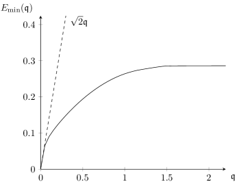
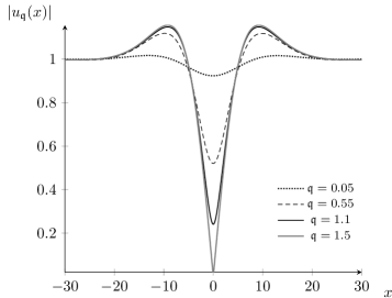
Figure 2: Curve $E_{\textup{min}}$ and solitons for the potential in (7.1), with $\alpha=0.05$ and $\beta=0.15$.

In both cases, we observe that $E_{\textup{min}}$ is concave and that the line $\sqrt{2}\mathfrak{q}$ is a tangent to the curve. We notice that the shapes of the solitons in Figure 3 and the solitons in Figure 1 are quite similar. On the other hand, the solitons in Figure 2 are very different, they have values greater than $1$ and exhibit a bump on $\mathbb{R}^{+}$. Notice also that the curves $E_{\textup{min}}$ for both potentials seem to be constant for $\mathfrak{q}>1.55$.

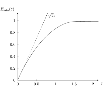
Figure 3: Curve $E_{\textup{min}}$ and solitons for the potential in (7.2), with $\alpha=0.8$.

We end this section showing some numerical simulations for two interesting potentials. The first one has been proposed in [58] as simple model for interactions in a Bose–Einstein condensate. It is given by a contact interaction $\delta_{0}$ and two Dirac delta functions centered at $\pm\sigma$,

$$\mathcal{W}_{\sigma}=2\delta_{0}-\frac{1}{2}\left(\delta_{\sigma}+\delta_{-\sigma}\right).$$ (7.3)

Noticing that $\widehat{\mathcal{W}}_{\sigma}(\xi)=2-\cos(\sigma\xi)$, we see that for $\sigma>0$, $\mathcal{W}_{\sigma}$ fulfills (H1), (H2), and that $\widehat{\mathcal{W}}_{\sigma}$ is analytic in $\mathbb{C}$, but is exponentially growing on $\mathbb{H}$. Thus, $\mathcal{W}_{\sigma}$ does not satisfy the assumption (5) in (H3). We can also check that (H3’) is not fulfilled. Nevertheless, the results of the simulation depicted in Figure 4 show that $E_{\textup{min}}$ is concave, and in that case Theorem 4 gives the orbital stability of the solitons illustrated in Figure 4.

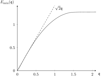
Figure 4: Curve $E_{\textup{min}}$ and solitons for the potential in (7.3), with $\sigma=10$.

Finally, we consider the potential

$$\widehat{\mathcal{W}}_{a,b,c}(\xi)=(1+a\xi^{2}+b\xi^{4})e^{-c\xi^{2}},$$ (7.4)

that it has been proposed in [9, 57] to describe a quantum fluid exhibiting a roton-maxon spectrum such as Helium 4. Indeed, as predicted by the Landau theory, in such a fluid, the dispersion curve (3) cannot be monotone and it should have a local maximum and a local minimum, that are the so-called maxon and roton, respectively. In Figure 5, we see the dispersion curve associated with potential (7.4), with $a=-36$, $b=2687$, $c=30$. In this case, there is a maxon at $\xi_{m}\sim 0.33$ and a roton at $\xi_{r}\sim 0.53$.

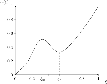
Figure 5: Dispersion curve associated with potential (7.4), with $a=-36$, $b=2687$, $c=30$. Here $\xi_{m}\sim 0.33$ and $\xi_{r}\sim 0.53$.

For these values, (H1) is satisfied, but not (H2) nor (H3’). However, we observe in Figure 6 that the energy curve is still concave, and that the straight line $\sqrt{2}\mathfrak{q}$ is still a tangent to the curve. Moreover, we found the same critical value as before for the momentum, i.e. $\mathfrak{q}_{*}\sim 1.55$.

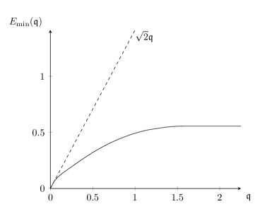
Figure 6: Curves $E_{\textup{min}}$ and solitons for the potential in (7.4), with $a=-36$, $b=2687$, $c=30$.

Acknowledgments.

The authors acknowledge support from the Labex CEMPI (ANR-11-LABX-0007-01). A. de Laire was also supported by the ANR project ODA (ANR-18-CE40-0020-01). The authors are grateful to S. De Bièvre and G. Dujardin for interesting and helpful discussions.

Appendix A Appendix

Lemma A.1.

Let $R>0$ and $\mu>0.$ There exists a function $\chi\in C^{\infty}_{c}(\mathbb{R})$ such that for all $x\in\mathbb{R}$, $0\leq\chi(x)\leq 1$,

$$\chi(x)=\begin{cases}1,&\text{ if }|x|\leq R,\\ 0,&\text{ if }|x|\geq R+\mu,\end{cases}\quad\text{and }\quad|\chi^{\prime}(x)|\leq 4e^{-2}e^{\frac{2}{\mu}}.$$ (A.1)

Proof.

Let

$$f(x):=\begin{cases}\exp(-\frac{1}{x}),&\text{ if }x\geq 0,\\ 0,&\text{ if }x<0,\end{cases}\quad\text{ and }\quad\chi(x):=\frac{f(R+\mu-|x|)}{f(R+\mu-|x|)+f(|x|-R)}.$$

Since

$$f(|x|-R)+f(R+\mu-|x|)\geq f(\frac{\mu}{2})=2e^{-\frac{2}{\mu}},$$ (A.2)

the denominator of $\chi$ is always positive, and thus $\chi$ is well defined. Moreover, $\chi\in C^{\infty}(\mathbb{R})$, since $f$ is smooth. Finally, for $|x|\leq R,$ we have $f(|x|-R)=0$, which implies that $\chi(x)=1.$ For $|x|\geq R+\mu$, we have $f(R+\mu-|x|)=0$, so that $\chi(x)=0.$

It remains to prove the bound in (A.1). Using that

$$\chi^{\prime}(x)=\frac{f^{\prime}(R+\mu-|x|)f(|x|-R)+f^{\prime}(|x|-R)f(R+\mu-|x|)}{(f(|x|-R)+f(R+\mu-|x|))^{2}},$$

and that $|f^{\prime}(x)|\leq\frac{\exp(-1/x)}{x^{2}}\leq 4e^{-2},$ we get

$$|\chi^{\prime}(x)|\leq\frac{8e^{-2}}{f(|x|-R)+f(R+\mu-|x|)}.$$

Combining with (A.2), we conclude that $|\chi^{\prime}(x)|\leq 4e^{-2}e^{\frac{2}{\mu}}$. ∎

References

- [1] M. Abid, C. Huepe, S. Metens, C. Nore, C. Pham, L. Tuckerman, and M. Brachet. Gross-Pitaevskii dynamics of Bose-Einstein condensates and superfluid turbulence. Fluid Dynamics Research, 33(5):509 – 544, 2003. Collection of Papers written by Regional Editors.
- [2] M. Abramowitz and I. A. Stegun. Handbook of mathematical functions with formulas, graphs, and mathematical tables, volume 55 of National Bureau of Standards Applied Mathematics Series. For sale by the Superintendent of Documents, U.S. Government Printing Office, Washington, D.C., 1964.
- [3] J. Albert. Positivity properties and uniqueness of solitary wave solutions of the intermediate long-wave equation. In Evolution equations (Baton Rouge, LA, 1992), volume 168 of Lecture Notes in Pure and Appl. Math., pages 11–20. Dekker, New York, 1995.
- [4] P. Antonelli and C. Sparber. Existence of solitary waves in dipolar quantum gases. Phys. D, 240(4-5):426–431, 2011.
- [5] C. Audiard. Small energy traveling waves for the Euler-Korteweg system. Nonlinearity, 30(9):3362–3399, 2017.
- [6] C. Becker, S. Stellmer, P. Soltan-Panahi, S. Dörscher, M. Baumert, E.-M. Richter, J. Kronjäger, K. Bongs, and K. Sengstock. Oscillations and interactions of dark and dark–bright solitons in Bose-Einstein condensates. Nature Physics, 4(6):496, 2008.
- [7] J. Bellazzini and L. Jeanjean. On dipolar quantum gases in the unstable regime. SIAM J. Math. Anal., 48(3):2028–2058, 2016.
- [8] N. G. Berloff. Quantum vortices, travelling coherent structures and superfluid turbulence. In Stationary and time dependent Gross-Pitaevskii equations, volume 473 of Contemp. Math., pages 27–54. Amer. Math. Soc., Providence, RI, 2008.
- [9] N. G. Berloff and P. H. Roberts. Motions in a Bose condensate VI. Vortices in a nonlocal model. J. Phys. A, 32(30):5611–5625, 1999.
- [10] F. Béthuel, P. Gravejat, and J.-C. Saut. Existence and properties of travelling waves for the Gross-Pitaevskii equation. In Stationary and time dependent Gross-Pitaevskii equations, volume 473 of Contemp. Math., pages 55–103. Amer. Math. Soc., Providence, RI, 2008.
- [11] F. Béthuel, P. Gravejat, and J.-C. Saut. Travelling waves for the Gross-Pitaevskii equation. II. Comm. Math. Phys., 285(2):567–651, 2009.
- [12] F. Béthuel, P. Gravejat, J.-C. Saut, and D. Smets. Orbital stability of the black soliton for the Gross-Pitaevskii equation. Indiana Univ. Math. J., 57(6):2611–2642, 2008.
- [13] F. Béthuel, P. Gravejat, J.-C. Saut, and D. Smets. On the Korteweg-de Vries long-wave approximation of the Gross-Pitaevskii equation. I. Int. Math. Res. Not. IMRN, (14):2700–2748, 2009.
- [14] F. Bethuel, P. Gravejat, and D. Smets. Asymptotic stability in the energy space for dark solitons of the Gross-Pitaevskii equation. Ann. Sci. Éc. Norm. Supér. (4), 48(6):1327–1381, 2015.
- [15] F. Bethuel, G. Orlandi, and D. Smets. Vortex rings for the Gross-Pitaevskii equation. J. Eur. Math. Soc. (JEMS), 6(1):17–94, 2004.
- [16] F. Béthuel and J.-C. Saut. Travelling waves for the Gross-Pitaevskii equation I. Ann. Inst. H. Poincaré Phys. Théor., 70(2):147–238, 1999.
- [17] M. Bogdan, A. Kovalev, and A. Kosevich. Stability criterion in imperfect Bose gas. Fiz. Nizk. Temp., 15(5):511–514, 1989. In Russian.
- [18] N. N. Bogoliubov. On the theory of superfluidity. J. Phys. USSR, 11:23–32, 1947. Reprinted in: D. Pines, The Many-Body Problem (W. A. Benjamin, New York, 1961), p. 292-301.
- [19] H. Brezis. Functional analysis, Sobolev spaces and partial differential equations. Universitext. Springer, New York, 2011.
- [20] R. Carles, P. A. Markowich, and C. Sparber. On the Gross-Pitaevskii equation for trapped dipolar quantum gases. Nonlinearity, 21(11):2569–2590, 2008.
- [21] T. Cazenave. Semilinear Schrödinger equations, volume 10 of Courant Lecture Notes in Mathematics. New York University Courant Institute of Mathematical Sciences, New York, 2003.
- [22] T. Cazenave and P.-L. Lions. Orbital stability of standing waves for some nonlinear Schrödinger equations. Comm. Math. Phys., 85(4):549–561, 1982.
- [23] D. Chiron. Travelling waves for the nonlinear Schrödinger equation with general nonlinearity in dimension one. Nonlinearity, 25(3):813–850, 2012.
- [24] D. Chiron. Stability and instability for subsonic traveling waves of the nonlinear Schrödinger equation in dimension one. Anal. PDE, 6(6):1327–1420, 2013.
- [25] D. Chiron and M. Mariş. Traveling waves for nonlinear Schrödinger equations with nonzero conditions at infinity. Arch. Ration. Mech. Anal., 226(1):143–242, 2017.
- [26] D. Chiron and F. Rousset. The KdV/KP-I limit of the nonlinear Schrödinger equation. SIAM J. Math. Anal., 42(1):64–96, 2010.
- [27] A. de Laire. Non-existence for travelling waves with small energy for the Gross-Pitaevskii equation in dimension . C. R. Math. Acad. Sci. Paris, 347(7-8):375–380, 2009.
- [28] A. de Laire. Global well-posedness for a nonlocal Gross-Pitaevskii equation with non-zero condition at infinity. Comm. Partial Differential Equations, 35(11):2021–2058, 2010.
- [29] A. de Laire. Nonexistence of traveling waves for a nonlocal Gross-Pitaevskii equation. Indiana Univ. Math. J., 61(4):1451–1484, 2012.
- [30] A. de Laire and P. Gravejat. Stability in the energy space for chains of solitons of the Landau-Lifshitz equation. J. Differential Equations, 258(1):1–80, 2015.
- [31] A. de Laire and P. Gravejat. The Sine-Gordon regime of the Landau-Lifshitz equation with a strong easy-plane anisotropy. Ann. Inst. H. Poincaré Anal. Non Linéaire, 35(7):1885–1945, 2018.
- [32] J. Denschlag, J. E. Simsarian, D. L. Feder, C. W. Clark, L. A. Collins, J. Cubizolles, L. Deng, E. W. Hagley, K. Helmerson, W. P. Reinhardt, et al. Generating solitons by phase engineering of a Bose-Einstein condensate. Science, 287(5450):97–101, 2000.
- [33] C. Gallo. The Cauchy problem for defocusing nonlinear Schrödinger equations with non-vanishing initial data at infinity. Comm. Partial Differential Equations, 33(4-6):729–771, 2008.
- [34] P. Gérard. The Gross-Pitaevskii equation in the energy space. In A. Farina and J.-C. Saut, editors, Stationary and time dependent Gross-Pitaevskii equations. Wolfgang Pauli Institute 2006 thematic program, January–December, 2006, Vienna, Austria, volume 473 of Contemporary Mathematics, pages 129–148. American Mathematical Society.
- [35] P. Gérard. The Cauchy problem for the Gross-Pitaevskii equation. Ann. Inst. H. Poincaré Anal. Non Linéaire, 23(5):765–779, 2006.
- [36] D. Gilbarg and N. S. Trudinger. Elliptic partial differential equations of second order. Classics in Mathematics. Springer-Verlag, Berlin, 2001. Reprint of the 1998 edition.
- [37] J. Ginibre and G. Velo. On a class of nonlinear Schrödinger equations with nonlocal interaction. Math. Z., 170(2):109–136, 1980.
- [38] L. Grafakos. Classical Fourier analysis, volume 249 of Graduate Texts in Mathematics. Springer, New York, second edition, 2008.
- [39] P. Gravejat and D. Smets. Asymptotic stability of the black soliton for the Gross-Pitaevskii equation. Proc. Lond. Math. Soc. (3), 111(2):305–353, 2015.
- [40] E. P. Gross. Hydrodynamics of a superfluid condensate. Journal of Mathematical Physics, 4(2):195–207, 1963.
- [41] S. Gustafson, K. Nakanishi, and T.-P. Tsai. Global dispersive solutions for the Gross-Pitaevskii equation in two and three dimensions. Ann. Henri Poincaré, 8(7):1303–1331, 2007.
- [42] S. Gustafson, K. Nakanishi, and T.-P. Tsai. Scattering theory for the Gross-Pitaevskii equation in three dimensions. Commun. Contemp. Math., 11(4):657–707, 2009.
- [43] Y. V. Kartashov and L. Torner. Gray spatial solitons in nonlocal nonlinear media. Opt. Lett., 32(8):946–948, 2007.
- [44] R. Killip, T. Oh, O. Pocovnicu, and M. Vişan. Global well-posedness of the Gross-Pitaevskii and cubic-quintic nonlinear Schrödinger equations with non-vanishing boundary conditions. Math. Res. Lett., 19(5):969–986, 2012.
- [45] T. Lahaye, C. Menotti, L. Santos, M. Lewenstein, and T. Pfau. The physics of dipolar bosonic quantum gases. Reports on Progress in Physics, 72(12):126401, 2009.
- [46] E. H. Lieb. Existence and uniqueness of the minimizing solution of Choquard’s nonlinear equation. Studies in Appl. Math., 57(2):93–105, 1976/77.
- [47] Z. Lin. Stability and instability of traveling solitonic bubbles. Adv. Differential Equations, 7(8):897–918, 2002.
- [48] P.-L. Lions. The concentration-compactness principle in the calculus of variations. The locally compact case. I. Ann. Inst. H. Poincaré Anal. Non Linéaire, 1(2):109–145, 1984.
- [49] O. Lopes and M. Mariş. Symmetry of minimizers for some nonlocal variational problems. J. Funct. Anal., 254(2):535–592, 2008.
- [50] Y. Luo and A. Stylianou. Ground states for a nonlocal cubic-quartic Gross-Pitaevskii equation. Preprint http://arxiv.org/abs/1806.00697.
- [51] M. Mariş. Traveling waves for nonlinear Schrödinger equations with nonzero conditions at infinity. Ann. of Math. (2), 178(1):107–182, 2013.
- [52] M. Mariş. On some minimization problems in . In New trends in differential equations, control theory and optimization, pages 215–230. World Sci. Publ., Hackensack, NJ, 2016.
- [53] M. Mariş. Nonexistence of supersonic traveling waves for nonlinear Schrödinger equations with nonzero conditions at infinity. SIAM J. Math. Anal., 40(3):1076–1103, 2008.
- [54] V. Moroz and J. Van Schaftingen. Groundstates of nonlinear Choquard equations: existence, qualitative properties and decay asymptotics. J. Funct. Anal., 265(2):153–184, 2013.
- [55] H. Pecher. Global solutions for 3D nonlocal Gross-Pitaevskii equations with rough data. Electron. J. Differential Equations, pages No. 170, 34, 2012.
- [56] L. P. Pitaevskii. Vortex lines in an imperfect Bose gas. Sov. Phys. JETP, 13(2):451–454, 1961.
- [57] J. Reneuve, J. Salort, and L. Chevillard. Structure, dynamics, and reconnection of vortices in a nonlocal model of superfluids. Phys. Rev. Fluids, 3(11):114602, 2018.
- [58] H. Veksler, S. Fishman, and W. Ketterle. Simple model for interactions and corrections to the Gross-Pitaevskii equation. Phys. Rev. A, 90(2):023620, 2014.
- [59] D. Vocke, T. Roger, F. Marino, E. M. Wright, I. Carusotto, M. Clerici, and D. Faccio. Experimental characterization of nonlocal photon fluids. Optica, 2(5):484–490, 2015.
- [60] V. Zakharov and E. Kuznetsov. Multi-scales expansion in the theory of systems integrable by the inverse scattering transform. Phys. D, 18(1-3):455–463, 1986.
- [61] P. E. Zhidkov. Korteweg-de Vries and nonlinear Schrödinger equations: qualitative theory, volume 1756 of Lecture Notes in Mathematics. Springer-Verlag, Berlin, 2001.