Core Decomposition in Multilayer Networks:
Theory, Algorithms, and Applications

Abstract.

Multilayer networks are a powerful paradigm to model complex systems, where multiple relations occur between the same entities. Despite the keen interest in a variety of tasks, algorithms, and analyses in this type of network, the problem of extracting dense subgraphs has remained largely unexplored so far.

As a first step in this direction, in this work we study the problem of core decomposition of a multilayer network. Unlike the single-layer counterpart in which cores are all nested into one another and can be computed in linear time, the multilayer context is much more challenging as no total order exists among multilayer cores; rather, they form a lattice whose size is exponential in the number of layers. In this setting we devise three algorithms which differ in the way they visit the core lattice and in their pruning techniques. We assess time and space efficiency of the three algorithms on a large variety of real-world multilayer networks.

We then move a step forward and study the problem of extracting the inner-most (also known as maximal) cores, i.e., the cores that are not dominated by any other core in terms of their core index in all the layers. Inner-most cores are typically orders of magnitude less than all the cores. Motivated by this, we devise an algorithm that effectively exploits the maximality property and extracts inner-most cores directly, without first computing a complete decomposition. This allows for a consistent speed up over a naïve method that simply filters out non-inner-most ones from all the cores.

Finally, we showcase the multilayer core-decomposition tool in a variety of scenarios and problems. We start by considering the problem of densest-subgraph extraction in multilayer networks. We introduce a definition of multilayer densest subgraph that trades-off between high density and number of layers in which the high density holds, and exploit multilayer core decomposition to approximate this problem with quality guarantees. As further applications, we show how to utilize multilayer core decomposition to speed-up the extraction of frequent cross-graph quasi-cliques and to generalize the community-search problem to the multilayer setting.

1. Introduction

In several real-world contexts, such as social media, biological networks, financial networks, transportation systems, it is common to encounter multiple relations among the objects of the underlying domain. Data in these scenarios is therefore modeled as a graph composed of a superimposition of different layers, i.e., where multiple edges of different types exist between a pair of vertices (Dickison et al., 2016; Cai et al., 2005; Lee et al., 2015). In the literature different terminologies have been used for graphs of this kind: multilayer networks, multiplex networks, multidimensional networks, multirelational networks, multislice networks, and more. No uniformity exists in this regard, and the various terms may also refer to slightly different concepts. In this work we deal with networks composed of multiple layers, with no inter-layer links, and hereinafter use the term “multilayer networks” to refer to them.

Extracting dense structures from large graphs has emerged as a key graph-mining primitive in a variety of scenarios (Lee et al., 2010), ranging from web mining (Gibson et al., 2005), to biology (Fratkin et al., 2006; Langston and et al., 2005), and finance (Du et al., 2009). Although the literature on multilayer graphs has grown fast in the last years, the problem of extracting dense subgraphs in this type of graph has remained, surprisingly, largely unexplored.

In single-layer graphs, among the many definitions of a dense structure, core decomposition plays a central role (Bonchi et al., 2018). The $k$-core of a graph is defined as a maximal subgraph in which every vertex has at least $k$ neighbors within that subgraph. The set of all $k$-cores of a graph $G$ forms the core decomposition of $G$ (Seidman, 1983). The appeal of core decomposition lies in the fact that it can be computed very fast, in linear time (Matula and Beck, 1983; Batagelj and Zaveršnik, 2011), while, at the same time, being easily used to speed-up/approximate dense-subgraph extraction according to various other definitions. For instance, core decomposition may speed up maximal-clique finding (Eppstein et al., 2010), as a $k$-clique is guaranteed to be contained into a $(k\!-\!1)$-core, which can be significantly smaller than the original graph. Moreover, core decomposition can be used to approximate betweenness centrality (Healy et al., 2006), and to design linear-time approximation algorithms for the densest-subgraph (Kortsarz and Peleg, 1994) and the densest at-least-$k$-subgraph (Andersen and Chellapilla, 2009) problems.

In this work we study the problem of core decomposition in multilayer networks. A major challenge with respect to the single-layer setting is that the number of multilayer cores is exponential in the number of layers. We achieve this challenge by devising a number of pruning techniques to avoid from-scratch computation of all the cores and exploit such techniques to devise efficient algorithms.

Nevertheless, computing multilayer core decomposition efficiently is not enough. Due the potentially high number of multilayer cores, a further major desideratum is to provide a data analyst with additional tools to browse through the output, and ultimately select the patterns of interest. The situation resembles that of the classic association-rule and frequent-itemset mining: a potentially exponential output, efficient algorithms to extract all the patterns, the need to have concise summaries of the extracted knowledge, and the opportunity of using the extracted patterns as building blocks for more sophisticated analyses. Following this direction, we present a number of problems and applications built on top of the multilayer core-decomposition tool. First we focus on the problem of extracting only the maximal or, as we call them in this work, the inner-most cores, i.e., cores that are not “dominated” by any other core. As experimentally observed, inner-most cores are orders of magnitude less than all the cores. Therefore, it is desirable to design algorithms that effectively exploit the maximality property and extract inner-most cores directly, without first computing a complete decomposition. Then, we show how multilayer core decomposition finds application to the problem of densest-subgraph extraction in multilayer networks (Jethava and Beerenwinkel, 2015; Charikar et al., 2018). As a further application, we exploit multilayer core decomposition to speed-up the extraction of frequent cross-graph quasi-cliques (Jiang and Pei, 2009). Finally, we exploit multilayer core decomposition to generalize the community-search problem (Sozio and Gionis, 2010) to the multilayer setting.

1.1. Background and related work

Core decomposition. Given a single-layer graph $G=(V,E)$ and a vertex $u\in V$, let $deg(u)$ and $deg_{S}(u)$ denote the degree of $u$ in $G$ and in a subgraph $S$ of $G$, respectively. Also, given a subset $C\subseteq V$ of vertices, let $E[C]$ denote the subset of edges induced by $C$.

Definition 1 (core decomposition).

The $k$-core (or core of order $k$) of a single-layer graph $G=(V,E)$ is a maximal subgraph $G[C_{k}]=(C_{k},E[C_{k}])$ such that $\forall u\in C_{k}:deg_{C_{k}}(u)\geq k$. The set $G=C_{0}\supseteq C_{1}\supseteq\cdots\supseteq C_{k^{*}}$ of all $k$-cores ($k^{*}=\arg\max_{k}C_{k}\neq\emptyset$) is the core decomposition of $G$.

Core decomposition can be computed in linear time by iteratively removing the smallest-degree vertex and setting its core number as its degree at the time of removal (Batagelj and Zaveršnik, 2011). Core decomposition has established itself as an important tool for network analysis and visualization (Batagelj et al., 1999; Alvarez-Hamelin et al., 2005) in several domains, e.g., bioinformatics (Bader and Hogue, 2003; Wuchty and Almaas, 2005), software engineering (Zhang et al., 2010), and social networks (Kitsak et al., 2010; García et al., 2013). It has been studied under various settings, such as distributed (Aksu et al., 2014; Khaouid et al., 2015; Montresor et al., 2013; Pechlivanidou et al., 2014), streaming (Li et al., 2014; Saríyüce et al., 2013; Zhang et al., 2017a), and external-memory (Cheng et al., 2011; Wen et al., 2016), and for various types of graph, such as uncertain (Bonchi et al., 2014), directed (Giatsidis et al., 2013), weighted (Garas et al., 2012), and attributed (Zhang et al., 2017b) graphs. Core decomposition has been studied also for temporal networks: (Wu et al., 2015a) defines the $(k,h)$-core, where $h$ accounts for the number of multiple temporal edges between two vertices of degree at least $k$, while (Galimberti et al., 2018) introduces the concept of (maximal) span-core, i.e., a core structure assigned with clear temporal collocation. See (Bonchi et al., 2018) for a comprehensive survey.

In this paper we adopt the definition of a multilayer core by Azimi-Tafreshi et al. (Azimi-Tafreshi et al., 2014), that is a core identified by an $|L|$-dimensional integer vector $\mathbf{k}$ (with $|L|$ being the number of layers of the given multilayer network), where every component of $\mathbf{k}$ refers to the minimum-degree constraint in the corresponding layer, i.e., $\mathbf{k}[i]$ states the minimum degree required for that core in the $i$-th layer, for all $i\in[1..|L|]$. Apart from introducing the multilayer-core definition, Azimi-Tafreshi et al. study the core-percolation problem from a physics standpoint, with no algorithmic contribution: they characterize cores of 2-layer Erdős-Rényi and scale-free networks, and observe how this characterization fits real-world air-transportation networks. To the best of our knowledge, no prior work has studied how to efficiently compute the complete core decomposition of multilayer networks.

Densest subgraph. Several notions of density exist in the literature, each of which leading to a different version of the dense-subgraph-discovery problem. While most variants are $\mathbf{NP}$-hard and/or inapproximable, extracting dense subgraphs according to the average-degree density is solvable in polynomial time (Goldberg, 1984). As a result, such a density has attracted most of the research in the field, so that the subgraph maximizing the average degree is commonly referred to as the densest subgraph. Goldberg (Goldberg, 1984) provides an exact algorithm for finding the densest subgraph which is based on iteratively solving ad-hoc-defined minimum-cut problem instances. Although principled, the Goldberg’s algorithm cannot scale to large graphs. Asahiro et al. (Asahiro et al., 2000) devises a linear-time greedy algorithm that has been shown to achieve $\frac{1}{2}$-approximation guarantee by Charikar (Charikar, 2000). Such a greedy algortihm iteratively removes the smallest-degree vertex, and, among all the subgraphs yielded during this vertex-removal process, the densest one is ultimately output. Note that this algorithm resembles the one used for core decomposition. In fact, it can be proved that the inner-most core of a graph is itself a $\frac{1}{2}$-approximation of the densest subgraph.

Variants of the densest-subgraph problem with size constraints turn out to be $\mathbf{NP}$-hard. For these variants, approximation algorithms and other theoretical results have been presented (Asahiro et al., 2002; Feige et al., 2001; Arora et al., 1995; Andersen and Chellapilla, 2009). A number of works focus on extracting a subgraph maximizing densities other than the average degree. For instance, Tsourakakis et al. (Tsourakakis et al., 2013) resort to the notion of quasi-clique, while Tsourakakis (Tsourakakis, 2015) and Wang et al. (Wang et al., 2010) focus on notions of density based on k-cliques and/or triangles. The densest-subgraph problem has also been studied in different settings, such as streaming/dynamic context (Bahmani et al., 2012; Bhattacharya et al., 2015; Epasto et al., 2015), and top-$k$ fashion (Balalau et al., 2015; Galbrun et al., 2016; Nasir et al., 2017).

Dense structures in multilayer networks. Several recent works have dealt with the problem of extracting dense subgraphs from a set of multiple graphs sharing the same vertex set, which is a setting equivalent to the multilayer one we study in this work. Jethava and Beerenwinkel (Jethava and Beerenwinkel, 2015) define the densest common subgraph problem, i.e., find a subgraph maximizing the minimum average degree over all input graphs, and devise a linear-programming formulation and a greedy heuristic for it. Reinthal et al. (Reinthal et al., 2016) provide a Lagrangian relaxation of the Jethava and Beerenwinkel’s linear program, which can be solved more efficiently. Semertzidis et al. (Semertzidis et al., 2019) introduce three more variants of the problem, whose goal is to maximize the average average degree, the minimum minimum degree, and the average minimum degree, respectively. They show that the average-average variant reduces to the traditional densest-subgraph problem, and the minimum-minimum variant is polynomial-time solvable by a simple adaptation of the algorithm for core decomposition. They also devise heuristics for the remaining two variants. Charikar et al. (Charikar et al., 2018) further focus on the minimum-average and average-minimum formulations, by providing several theoretical findings, including $\mathbf{NP}$-hardness, hardness of the approximation (for both minimum-average and average-minimum), an integrality gap for the linear-programming relaxation introduced in (Jethava and Beerenwinkel, 2015; Reinthal et al., 2016) (for minimum-average), and a characterization in terms of parameterized complexity (for average-minimum).

Other contributions in this area, less directly related to our work, deal with specific cases of 2-layer networks (Wu et al., 2015b; Shen et al., 2015) and with the community-detection problem (Berlingerio et al., 2011; Mucha et al., 2010; Papalexakis et al., 2013; Cai et al., 2005; Tagarelli et al., 2017; Tang et al., 2010; Yin and Khaing, 2013). Boden et al. (Boden et al., 2012) study subspace clustering for multilayer graphs, i.e., find clusters of vertices that are densely connected by edges with similar labels for all possible label sets. Yan et al. (Yan et al., 2005) introduce the problem of mining closed relational graphs, i.e., frequent subgraphs of a multilayer graph exhibiting large minimum cut. Jiang et al. (Jiang and Pei, 2009) focus on extracting frequent cross-graph quasi-cliques, i.e., subgraphs that are quasi-cliques in at least a fraction of layers equal to a certain minimum support and have size larger than a given threshold. Interdonato et al. (Interdonato et al., 2017) are the first to study the problem of local community detection in multilayer networks, i.e., when a seed vertex is given and the goal is to reconstruct its community by having only a limited local view of the network. Finally, Zhu et al. (Zhu et al., 2018) address the problem of finding the $k$ most diversified $d$-coherent cores, i.e., the $k$ subgraphs having minimum degree at least $d$ that maximize the coverage of the vertices.

In this work, in Section 5, we introduce a formulation of the densest-subgraph problem in multilayer networks that trades off between high density and number of layers where the high density holds. We apply multilayer core decomposition to provide provable approximation guarantees for this problem. We also show that our formulation generalizes the minimum-average densest-common-subgraph problem studied in (Charikar et al., 2018; Jethava and Beerenwinkel, 2015; Reinthal et al., 2016; Semertzidis et al., 2019), and our method achieves approximation guarantees for that problem too. Furthermore, in Section 6, we show how to exploit multilayer core decomposition to speed-up the problem of finding frequent cross-graph quasi-cliques (Jiang and Pei, 2009).

Community search. Given a (single-layer) graph and a set of query vertices, the community search problem aims at finding a cohesive subgraph containing the query vertices. Community search has received a great deal of attention in the data-mining community in the last few years (see e.g., a recent tutorial (Huang et al., 2017)). Sozio and Gionis (Sozio and Gionis, 2010) are the first to introduce the community-search problem, by employing the minimum degree as a cohesiveness measure. Their formulation can be solved by a simple (linear-time) greedy algorithm, which is very similar to the one proposed in (Charikar, 2000) for the densest-subgraph problem. More recently, Cui et al. (Cui et al., 2014) devise a local-search approach to improve the efficiency of the method defined in (Sozio and Gionis, 2010), but only for the special case of a single query vertex. The minimum-degree-based problem has been further studied in (Barbieri et al., 2015), by exploiting core decomposition as a preprocessing step to allow more efficient and effective solutions.

Several formulations of the community search have also been studied under different names and in slightly different settings. Andersen and Lang (Andersen and Lang, 2006) and Kloumann and Kleinberg (Kloumann and Kleinberg, 2014) study seed set expansion in social graphs, in order to find communities with small conductance or that are well-resemblant of the characteristics of the query vertices, respectively. Other works define connectivity subgraphs based on electricity analogues (Faloutsos et al., 2004), random walks (Tong and Faloutsos, 2006), the minimum-description-length principle (Akoglu et al., 2013), the Wiener index (Ruchansky et al., 2015), and network efficiency (Ruchansky et al., [n. d.]). Community search has been formalized for attributed (Huang and Lakshmanan, 2017; Fang et al., 2017a) and spatial graphs (Fang et al., 2017b) as well.

In this work, in Section 7, we formulate the community-search problem for multilayer graphs, by adapting the early definition by Sozio and Gionis (Sozio and Gionis, 2010), and show how our algorithms for multilayer core decomposition can be exploited to obtain optimal solutions to this problem.

1.2. Challenges, contributions, and roadmap

Let $G=(V,E,L)$ be a multilayer graph, where $V$ is a set of vertices, $L$ is a set of layers, and $E\subseteq V\times V\times L$ is a set of edges. Given an $|L|$-dimensional integer vector $\mathbf{k}=[k_{\ell}]_{\ell\in L}$, the multilayer $\mathbf{k}$-core of $G$ is a maximal subgraph whose vertices have at least degree $k_{\ell}$ in that subgraph, for all layers $\ell\in L$ (Azimi-Tafreshi et al., 2014). Vector $\mathbf{k}$ is dubbed coreness vector of that core. The set of all non-empty and distinct multilayer cores constitutes the multilayer core decomposition of $G$. A major challenge of computing the core decomposition of a multilayer network is that the number of multilayer cores are exponential in the number of layers. This makes the problem inherently hard, as the exponential size of the output clearly precludes the existence of polynomial-time algorithms in the general case. In fact, unlike the single-layer case where cores are all nested into each other, no total order exists among multilayer cores. Rather, they form a core lattice defining partial containment. As a result, algorithms in the multilayer setting must be crafted carefully to handle this exponential blowup, and avoid, as much as possible, the computation of unnecessary (i.e., empty or non-distinct) cores.

A naïve way of computing a multilayer core decomposition consists in generating all coreness vectors, run for each vector $\mathbf{k}$, an algorithm that iteratively removes vertices whose degree in a layer $\ell$ is less than the $\ell$-th component of $\mathbf{k}$, and filter out empty and duplicated cores. This method has evident efficiency issues, as every core is computed from the whole input graph, and it does not avoid generation of empty or non-distinct cores at all. As our first contribution, we devise three more efficient algorithms that exploit effective pruning rules during the visit of the lattice. The first two methods are based on a bfs and a dfs strategy, respectively: the bfs method exploits the fact that a core is contained into the intersection of all its fathers in the lattice, while the dfs method iteratively performs a single-layer core decomposition to compute, one-shot, all cores along a path from a non-leaf lattice core to a leaf. The third method adopts a hybrid strategy embracing the main pros of bfs and dfs, and equipped with a look-ahead mechanism to skip non-distinct cores.

We then shift the attention to the problem of computing all and only the inner-most cores, i.e., the cores that are not dominated by any other core in terms of their index on all the layers. A straightforward way of approaching this problem would be to first compute the complete core decomposition, and then filter out the non-inner-most cores. However, as the inner-most cores are usually much less than the overall cores, it would be desirable to have a method that effectively exploits the maximality property and extracts the inner-most ones directly, without computing a complete decomposition. The design of an algorithm of this kind is an interesting challenge, as it contrasts the intrinsic conceptual properties of core decomposition, based on which a core of order $k$ (in one layer) can be efficiently computed from the core of order $k-1$, of which it is a subset, thus naturally suggesting a bottom-up discovery. For this reason, at first glance, the computation of the core of the highest order would seem as hard as computing the overall core decomposition. In this work we show that, by means of a clever core-lattice visiting strategy, we can prune huge portions of the search space, thus achieving higher efficiency than computing the whole decomposition.

As a major application of multilayer core decomposition, we then focus on the problem of extracting the densest subgraph from a multilayer network. As already discussed in Section 1.1, a number of works aim at extracting a subgraph that maximizes the minimum average degree over all layers (Charikar et al., 2018; Jethava and Beerenwinkel, 2015; Reinthal et al., 2016; Semertzidis et al., 2019). A major limitation of that formulation is that, considering all layers, even the noisy/insignificant ones would contribute to selecting the output subgraph, which might prevent us from finding a subgraph being dense in a still large subset of layers. Another simplistic approach at the other end of the spectrum corresponds to flattening the input multilayer graph and resorting to single-layer densest-subgraph extraction. However, this would mean disregarding the different semantics of the layers, incurring in a severe information loss. Within this view, in this work we generalize the problem studied in (Charikar et al., 2018; Jethava and Beerenwinkel, 2015; Reinthal et al., 2016; Semertzidis et al., 2019) by introducing a formulation that accounts for a trade-off between high density and number of layers exhibiting the high density. Specifically, given a multilayer graph $G=(V,E,L)$, the average-degree density of a subset of vertices $S$ in a layer $\ell$ is defined as the number of edges induced by $S$ in $\ell$ divided by the size of $S$, i.e., $\frac{|E_{\ell}[S]|}{|S|}$. We define the multilayer densest subgraph as the subset of vertices $S^{*}$ such that the function

$$\max_{\hat{L}\subseteq L}\min_{\ell\in\hat{L}}\frac{\textstyle|E_{\ell}[S^{*}]|}{\textstyle|S^{*}|}{\textstyle|\hat{L}|^{\beta}}$$

is maximized. Parameter $\beta\in\mathbb{R}^{+}$ controls the importance of the two problem ingredients, i.e., high density and number of high-density layers. This problem statement naturally achieves the aforementioned desired trade-off: the larger the subset $\hat{L}$ of selected layers, the smaller the minimum density $\min_{\ell\in\hat{L}}\frac{|E_{\ell}[S]|}{|S|}$ in those layers. Similarly to the single-layer case where core decomposition provides a $\frac{1}{2}$-approximation of the densest subgraph, in this work we show that computing the multilayer core decomposition of the input graph and selecting the core maximizing the proposed multilayer density function achieves a $\frac{1}{2|L|^{\beta}}$-approximation for the general multilayer-densest-subgraph problem formulation, and a $\frac{1}{2}$-approximation for the all-layer variant in (Charikar et al., 2018; Jethava and Beerenwinkel, 2015; Reinthal et al., 2016; Semertzidis et al., 2019).

As a further application of multilayer core decomposition, we show how it can speed up frequent cross-graph quasi-clique extraction (Jiang and Pei, 2009). We prove that searching for frequent cross-graph quasi-cliques in restricted areas of the graph – corresponding to multilayer cores complying with the quasi-clique condition – is still sound and complete, while also being much more efficient.

Finally, we also provide a generalization of the community-search problem (Sozio and Gionis, 2010) to the multilayer setting, and show how to exploit multilayer core decomposition to optimally solve this problem.

Summarizing, this work has the following contributions:

1. We define the problem of core decomposition in multilayer networks, and characterize it in terms of relation to other problems, and complexity. We devise three algorithms that solve multilayer core decomposition efficiently (Section 3).

2. We devise further algorithms to compute the inner-most cores only (Section 4).

3. We study the problem of densest-subgraph in multilayer networks. We introduce a formulation that trades-off between high density and number of layers exhibiting high density, and exploit multilayer core decomposition to solve it with approximation guarantees (Section 5).

4. We show how the multilayer core-decomposition tool can be exploited to speed up the extraction of frequent cross-graph quasi-cliques (Section 6).

5. We formulate the multilayer community-search problem and show that multilayer core decomposition provides an optimal solution to this problem (Section 7).

We also provide extensive experiments, on numerous real datasets, to assess the performance of our proposals. For each aforementioned context, experiments are provided within the corresponding section. A preliminary version of this work, covering Sections 3 and 5 only, was presented in (Galimberti et al., 2017).

Reproducibility. For the sake of reproducibility all our code and some of the datasets used in this paper are available at https://github.com/egalimberti/multilayer_core_decomposition

2. Preliminaries and problem statements

In this section we introduce the needed preliminaries and notation, we provide some fundamental properties of multilayer cores, and then formally define all the problems studied in this work.

2.1. Multilayer core decomposition

We are given an undirected multilayer graph $G=(V,E,L)$, where $V$ is a set of vertices, $L$ is a set of layers, and $E\subseteq V\times V\times L$ is a set of edges. Let $E_{\ell}$ denote the subset of edges in layer $\ell\in L$. For a vertex $u\in V$ we denote by $\mbox{$deg$}(u,\ell)$ and $\mbox{$deg$}(u)$ its degree in layer $\ell$ and over all layers, respectively, i.e., $\mbox{$deg$}(u,\ell)=|\{e=(u,v,\ell):e\in E_{\ell}\}|$, $\mbox{$deg$}(u)=|\{e=(u,v,\ell):e\in E\}|=\sum_{\ell\in L}\mbox{$deg$}(u,\ell)$.

For a subset of vertices $S\subseteq V$ we denote by $G[S]$ the subgraph of $G$ induced by $S$, i.e., $G[S]=(S,E[S],L)$, where $E[S]=\{e=(u,v,\ell)\mid e\in E,u\in S,v\in S\}$. For a vertex $u\in V$ we denote by $\mbox{$deg$}_{S}(u,\ell)$ and $\mbox{$deg$}_{S}(u)$ its degree in subgraph $S$ considering layer $\ell$ only and all layers, respectively, i.e., $\mbox{$deg$}_{S}(u,\ell)=|\{e=(u,v,\ell):e\in E_{\ell}[S]\}|$, $\mbox{$deg$}_{S}(u)=|\{e=(u,v,\ell):e\in E[S]\}|=\sum_{\ell\in L}\mbox{$deg$}_{S}(u,\ell)$. Finally, let $\mu(\ell)$ and $\mu(\hat{L})$ denote the minimum degree of a vertex in layer $\ell$ and in a subset $\hat{L}\subseteq L$ of layers, respectively. Let also $\mu(S,\ell)$ and $\mu(S,\hat{L})$ denote the corresponding counterparts of $\mu(\ell)$ and $\mu(\hat{L})$ for a subgraph (induced by a vertex set) $S$.

A core of a multilayer graph is characterized by an $|L|$-dimensional integer vector $\mathbf{k}=[k_{\ell}]_{\ell\in L}$, termed coreness vector, whose components $k_{\ell}$ denote the minimum degree allowed in layer $\ell$. This corresponds to the notion of $\mathbf{k}$-core introduced by Azimi-Tafreshi et al. (Azimi-Tafreshi et al., 2014).As discussed in Section 1.1, Azimi-Tafreshi et al. do not study (or devise any algorithm for) the problem of computing the entire multilayer core decomposition. They study core percolation by analyzing a single core of interest, computed with the simple iterative-peeling algorithm (Algorithm 1). Formally:

Definition 2 (multilayer core and coreness vector (Azimi-Tafreshi et al., 2014)).

Given a multilayer graph $G=(V,E,L)$ and an $|L|$-dimensional integer vector $\mathbf{k}=[k_{\ell}]_{\ell\in L}$, the multilayer $\mathbf{k}$-core of $G$ is a maximal subgraph $G[C]=(C\subseteq V,E[C],L)$ such that $\forall\ell\in L:\mu(C,\ell)\geq k_{\ell}$. The vector $\mathbf{k}$ is referred to as the coreness vector of $G[C]$.

Given a coreness vector $\mathbf{k}$, we denote by $C_{\mathbf{k}}$ the corresponding core. Also, as a $\mathbf{k}$-core is fully identified by the vertices belonging to it, we hereinafter refer to it by its vertex set $C_{\mathbf{k}}$ and the induced subgraph $G[C_{\mathbf{k}}]$ interchangeably. It is important noticing that a set of vertices $C\subseteq V$ may correspond to multiple cores. For instance, in the graph in Figure 1 the set $\{\mbox{{A,B,D,E}}\}$ corresponds to both $(3,0)$-core and $(3,1)$-core. In other words, a multilayer core can be described by more than one coreness vector. However, as formally shown next, among such multiple coreness vectors there exists one and only one that is not dominated by any other. We call this vector the maximal coreness vector of $C$. In the example in Figure 1 the maximal coreness vector of $\{\mbox{{A,B,D,E}}\}$ is $(3,1)$.

Definition 3 (maximal coreness vector).

Let $G=(V,E,L)$ be a multilayer graph, $C\subseteq V$ be a core of $G$, and $\mathbf{k}=[k_{\ell}]_{\ell\in L}$ be a coreness vector of $C$. $\mathbf{k}$ is said maximal if there does not exist any coreness vector $\mathbf{k^{\prime}}=[k^{\prime}_{\ell}]_{\ell\in L}$ of $C$ such that $\forall\ell\in L:k^{\prime}_{\ell}\geq k_{\ell}$ and $\exists\hat{\ell}\in L:k^{\prime}_{\hat{\ell}}>k_{\hat{\ell}}$.

Figure 1. Example 2-layer graph (solid edges refer to the first layer, while dashed edges to the second layer) with the following $\mathbf{k}$-cores: $(0,0)=(1,0)=(0,1)=(1,1)=\{\mbox{{A,B,C,D,E,F}}\},(2,0)=(2,1)=\{\mbox{{A,B,D,E,F}}\},(3,0)=(3,1)=\{\mbox{{A,B,D,E}}\},(0,2)=(1,2)=(0,3)=(1,3)=\{\mbox{{B,C,E,F}}\},(2,2)=\{\mbox{{B,E,F}}\}$ .

Theorem 1.

Multilayer cores have a unique maximal coreness vector.

Proof.

We prove the theorem by contradiction. Assume two maximal coreness vectors $\mathbf{k}=[k_{\ell}]_{\ell\in L}\neq\mathbf{k}^{\prime}=[k^{\prime}_{\ell}]_{\ell\in L}$ exist for a multilayer core $C$. As $\mathbf{k}\neq\mathbf{k}^{\prime}$ and they are both maximal, there exist two layers $\hat{\ell}$ and $\bar{\ell}$ such that $k_{\hat{\ell}}>k^{\prime}_{\hat{\ell}}$ and $k^{\prime}_{\bar{\ell}}>k_{\bar{\ell}}$. By definition of multilayer core (Definition 2), it holds that $\forall\ell\in L:\mu(C,\ell)\geq k_{\ell},\mu(C,\ell)\geq k^{\prime}_{\ell}$. This means that the vector $\mathbf{k}^{*}=[k^{*}_{\ell}]_{\ell\in L}$, with $k^{*}_{\ell}=\max\{k_{\ell},k^{\prime}_{\ell}\},\forall\ell\in L$, is a further coreness vector of $C$. For this vector it holds that $\forall\ell\neq\hat{\ell},\ell\neq\bar{\ell}:k^{*}_{\ell}\geq k^{\prime}_{\ell}$, $k^{*}_{\hat{\ell}}>k^{\prime}_{\hat{\ell}}$, and $k^{*}_{\bar{\ell}}>k_{\bar{\ell}}$. Thus, $\mathbf{k}^{*}$ dominates both $\mathbf{k}$ and $\mathbf{k}^{\prime}$, which contradicts the hypothesis of maximality of $\mathbf{k}$ and $\mathbf{k}^{\prime}$. The theorem follows. ∎

The first (and main) problem we tackle in this work is the computation of the complete multilayer core decomposition, i.e., the set of all non-empty multilayer cores.

Problem 1 (Multilayer Core Decomposition).

Given a multilayer graph $G=(V,E,L)$, find the set of all non-empty and distinct cores of $G$, along with their corresponding maximal coreness vectors. Such a set forms what we hereinafter refer to as the multilayer core decomposition of $G$.

2.2. Inner-most multilayer cores

Cores of a single-layer graph are all nested one into another. This makes it possible to define the notions of $(i)$ inner-most core, as the core of highest order, and $(ii)$ core index (or core number) of a vertex $u$, which is the highest order of a core containing $u$. In the multilayer setting the picture is more complex, as multilayer cores are not all nested into each other. As a result, the core index of a vertex is not unambiguously defined, while there can exist multiple inner-most cores:

Definition 4 (inner-most multilayer cores).

The inner-most cores of a multilayer graph are all those cores with maximal coreness vector $\mathbf{k}=[k_{\ell}]_{\ell\in L}$ such that there does not exist any other core with coreness vector  $\mathbf{k}^{\prime}=[k^{\prime}_{\ell}]_{\ell\in L}$ where $\forall\ell\in L:k^{\prime}_{\ell}\geq k_{\ell}$ and $\exists\hat{\ell}\in L:k^{\prime}_{\hat{\ell}}>k_{\hat{\ell}}$.

To this purpose, look at the example in Figure 1. It can be observed that: ($i$) cores are not nested into each other, ($ii$) $(3,1)$-core, $(1,3)$-core and $(2,2)$-core are the inner-most cores, and ($iii$) vertices B and E belong to (inner-most) cores $(3,1)$, $(1,3)$, and $(2,2)$, thus making their core index not unambiguously defined.

The second problem we tackle in this work is the development of smart algorithms to compute all the inner-most cores, without the need of computing the complete multilayer core decomposition.

Problem 2 (Inner-most cores computation).

Given a multilayer graph $G=(V,E,L)$, find all non-empty and inner-most cores of $G$, along with their corresponding maximal coreness vectors.

2.3. Multilayer densest subgraph

As anticipated in Section 1.2, the densest subgraph of a multilayer graph should provide a good trade-off between large density and the number of layers where such a large density is exhibited. We achieve this intuition by means of the following optimization problem:

Problem 3 (Multilayer Densest Subgraph).

Given a multilayer graph $G=(V,E,L)$, a positive real number $\beta$, and a real-valued function $\delta:2^{V}\rightarrow\mathbb{R}^{+}$ defined as:

(1) $$\delta(S)=\max_{\hat{L}\subseteq L}\min_{\ell\in\hat{L}}\frac{|E_{\ell}[S]|}{|S|}|\hat{L}|^{\beta},$$

find a subset $S^{*}\subseteq V$ of vertices that maximizes function $\delta$, i.e.,

$$S^{*}=\arg\max_{S\subseteq V}\delta(S).$$

Parameter $\beta$ controls the importance of the two ingredients of the objective function $\delta$, i.e., density and number of layers exhibiting such a density: the smaller $\beta$, the better the focus on the former aspect (density), and vice versa. Also, as a nice side effect, solving Multilayer Densest Subgraph  allows for automatically finding a set of layers of interest for the densest subgraph $S^{*}$. In Section 5 we will show how to exploit it to devise an algorithm with approximation guarantees for Multilayer Densest Subgraph, thus extending to the multilayer case the intuition at the basis of the well-known $\frac{1}{2}$-approximation algorithm (Asahiro et al., 2000; Charikar, 2000) for single-layer densest subgraph.

2.4. Frequent cross-graph quasi-cliques

Another interesting insight into the notion of multilayer cores is about their relationship with (quasi-)cliques. In single-layer graphs it is well-known that cores can speed-up clique finding, as a clique of size $k$ is contained in the $(k-1)$-core. Interestingly, a similar relationship holds in the multilayer context too. Given a multilayer graph $G=(V,E,L)$, a layer $\ell\in L$, and a real number $\gamma\in(0,1]$, a subgraph $G[S]=(S\subseteq V,E[S],L)$ of $G$ is said to be a $\gamma$-quasi-clique in layer $\ell$ if all its vertices have at least $\gamma(|S|-1)$ neighbors in layer $\ell$ within $S$, i.e., $\forall u\in S:deg_{S}(u,\ell)\geq\gamma(|S|-1)$. Jiang et al. (Jiang and Pei, 2009) study the problem of extracting frequent cross-graph quasi-cliques, defined next.

Problem 4 (Frequent cross-graph quasi-cliques mining (Jiang and Pei, 2009)).

Given a multilayer graph $G=(V,E,L)$, a function $\Gamma:L\rightarrow(0,1]$ assigning a real value to every layer in $L$, a real number $\mbox{\emph{min\_sup}}\in(0,1]$, and an integer $\mbox{\emph{min\_size}}\geq 1$, find all maximal subgraphs $G[S]$ of $G$ of size larger than min_size such that there exist at least $\mbox{\emph{min\_sup}}\times|L|$ layers $\ell$ for which $G[S]$ is a $\Gamma(\ell)$-quasi-clique.

In Section 6 we will prove that a frequent cross-graph quasi-clique of size $K$ is necessarily contained into a $\mathbf{k}$-core described by a maximal coreness vector $\mathbf{k}=[k_{\ell}]_{\ell\in L}$ such that there exists a fraction of at least min_sup layers $\ell$ where $k_{\ell}=\lfloor\Gamma(\ell)(K-1)\rfloor$. Based on this, exploiting multilayer core decomposition as a preprocessing step allows for speeding up any algorithm for Problem 4.

2.5. Multilayer community search

The last application we study is the problem of community search. Given a graph $G=(V,E)$ and a set $V_{Q}\subseteq V$ of query vertices, a very wide family of problem requires to find a connected subgraph $H$ of $G$, which contains all query vertices $V_{Q}$ and exhibits an adequate degree of cohesiveness, compactness, or density. This type of problem has been termed in the literature in different ways, e.g., community search (Sozio and Gionis, 2010; Cui et al., 2014; Barbieri et al., 2015), seed set expansion (Andersen and Lang, 2006; Kloumann and Kleinberg, 2014), connectivity subgraphs (Faloutsos et al., 2004; Tong and Faloutsos, 2006; Ruchansky et al., 2015; Akoglu et al., 2013; Ruchansky et al., [n. d.]), just to mention a few: see (Huang et al., 2017) for a recent survey. In this work we adopt the early definition by Sozio and Gionis (Sozio and Gionis, 2010) which measures the cohesiveness of the resulting subgraph by means of the minimum degree inside the subgraph, and we adapt it to the multilayer setting as follows.

Problem 5 (Multilayer Community Search).

Given a multilayer graph $G=(V,E,L)$, a set $S\subseteq V$ of vertices, and a set $\hat{L}\subseteq L$ of layers, the minimum degree in the subgraph induced by $S$ and $\hat{L}$ is:

$$\varphi(S,\hat{L})=\min_{\ell\in\hat{L}}\min_{u\in S}deg_{S}(u,\ell).$$

Given a positive real number $\beta$, we define a real-valued density function $\vartheta:2^{V}\rightarrow\mathbb{R}^{+}$ as:

$$\vartheta(S)=\max_{\hat{L}\subseteq L}\varphi(S,\hat{L})|\hat{L}|^{\beta}.$$

Given a set $V_{Q}\subseteq V$ of query vertices, find a subgraph containing all the query vertices and maximizing the density function, i.e.,

(2) $$S^{*}=\operatorname*{arg\,max}_{V_{Q}\subseteq S\subseteq V}\vartheta(S).$$

In Section 7 we will show how to adapt multilayer core decomposition to solve Problem 5.

3. Algorithms for multilayer core decomposition

A major challenge of Multilayer Core Decomposition is that the number of multilayer cores may be exponential in the number of layers. Specifically, denoting by $K_{\ell}$ the maximum order of a core for layer $\ell$, the number of multilayer cores is $\mathcal{O}(\prod_{\ell\in L}K_{\ell})$. This makes Multilayer Core Decomposition intrinsically hard: in the general case, no polynomial-time algorithm can exist. The challenge hence lies in handling this exponential blowup by early recognizing and skipping unnecessary portions of the search space, such as non-distinct and/or empty cores.

Given a multilayer graph $G=(V,E,L)$ and a coreness vector $\mathbf{k}=[k_{\ell}]_{\ell\in L}$, finding the corresponding core can easily be solved in $\mathcal{O}(|E|+|V|\times|L|)$ time by iteratively removing a vertex $u$ having $\mbox{$deg$}_{G^{\prime}}(u,\ell)<k_{\ell}$ in some layer $\ell$, where $G^{\prime}$ denotes the current graph resulting from all previous vertex removals (Algorithm 1, where the set $S$ of vertices to be considered is set to $S=V$). Hence, a naïve way of computing a multilayer core decomposition consists of generating all possible coreness vectors, run the multilayer core-detection algorithm just described for each vector, and retain only non-empty and distinct cores. This naïve method requires all vectors $[k_{\ell}]_{\ell\in L}$, where each $k_{\ell}$ component is varied within the interval $[0..K_{\ell}]$. This corresponds to a $\Theta(\prod_{\ell\in L}K_{\ell})$ number of vectors. As a result, the overall time complexity of the method is $\mathcal{O}\big{(}(|E|+|V|\times|L|)\times\prod_{\ell\in L}K_{\ell}\big{)}$.

This approach has two major weaknesses: ($i$) each core is computed starting from the whole input graph, and ($ii$) by enumerating all possible coreness vectors beforehand a lot of non-distinct and/or empty (thus, unnecessary) cores may be computed. In the following we present three methods that solve Multilayer Core Decomposition much more efficiently.

Figure 2. Core lattice of a 3-layer graph.

3.1. Search space

Although multilayer cores are not all nested into each other, a notion of partial containment can still be defined. Indeed, it can easily be observed that a $\mathbf{k}$-core with coreness vector $\mathbf{k}=[k_{\ell}]_{\ell\in L}$ is contained into any $\mathbf{k}^{\prime}$-core described by a coreness vector $\mathbf{k}^{\prime}=[k^{\prime}_{\ell}]_{\ell\in L}$ whose components $k^{\prime}_{\ell}$ are all no more than components $k_{\ell}$, i.e., $k^{\prime}_{\ell}\leq k_{\ell}$, $\forall\ell\in L$. This result is formalized next:

Fact 1.

Given a multilayer graph $G=(V,E,L)$ and two cores $C_{\mathbf{k}}$ and $C_{\mathbf{k^{\prime}}}$ of $G$ with coreness vectors $\mathbf{k}=[k_{\ell}]_{\ell\in L}$ and $\mathbf{k}^{\prime}=[k^{\prime}_{\ell}]_{\ell\in L}$, respectively, it holds that if $\forall\ell\in L:k^{\prime}_{\ell}\leq k_{\ell}$, then $C_{\mathbf{k}}\subseteq C_{\mathbf{k^{\prime}}}$.

Proof.

Combining the definition of multilayer core (Definition 2) and the hypothesis on vectors $\mathbf{k}$ and $\mathbf{k}^{\prime}$, it holds that $\forall\ell\in L:\mu(C_{\mathbf{k}},\ell)\geq k_{\ell}\geq k^{\prime}_{\ell}$. This means that $C_{\mathbf{k}}$ satisfies the definition of $\mathbf{k}^{\prime}$-core, thus implying that all vertices in $C_{\mathbf{k}}$ are part of $C_{\mathbf{k}^{\prime}}$ too. The fact follows. ∎

Based on Fact 1, the search space of our problem can be represented as a lattice defining a partial order among all cores (Figure 2). Such a lattice, which we call the core lattice, corresponds to a dag where nodes represent cores, and links represent relationships of containment between cores (a “father” node contains all its “child” nodes). We assume the core lattice keeping track of non-empty and not necessarily distinct cores: a core is present in the lattice as many times as the number of its coreness vectors. Each level $i$ of the lattice represents the children of cores at lattice level $i-1$. In particular, level $i$ contains all those cores whose coreness vector results from increasing one and only one component of its fathers’ coreness vector by one. Formally, a lattice level $i$ contains all $\mathbf{k}$-cores with coreness vector $\mathbf{k}=[k_{\ell}]_{\ell\in L}$ such that there exists a core at lattice level $i-1$ with coreness vector $\mathbf{k}^{\prime}=[k^{\prime}_{\ell}]_{\ell\in L}$ where: $\exists\ell\in L:k_{\ell}=k^{\prime}_{\ell}+1$, and $\forall\hat{\ell}\neq\ell:k_{\hat{\ell}}=k^{\prime}_{\hat{\ell}}$. As a result, level 0 contains the root only, which corresponds to the whole input graph (i.e., the $[0]_{|L|}$-core), the leaves correspond to inner-most cores, and any non-leaf node has at least one and at most $\left|L\right|$ children. Moreover, every level $i$ contains all cores whose coreness-vector components sum to $i$.

Solving the Multilayer Core Decomposition problem is hence equivalent to building the core lattice of the input graph. The efficient methods we present next are all based on smart core-lattice building strategies that extract cores from smaller subgraphs, while also attempting to minimize the visit/computation of unnecessary (i.e., empty/non-distinct) cores.

Algorithm 1 $\mathbf{k}$-core

0:  A multilayer graph $G=(V,E,L)$, a set $S\subseteq V$ of vertices, an $|L|$-dimensional integer vector $\mathbf{k}=[k_{\ell}]_{\ell\in L}$.

0:  The $\mathbf{k}$-core $C_{\mathbf{k}}$ of $G$.

1:  while $\exists u\in S,\exists\ell\in L:\mbox{$deg$}_{S}(u,\ell)<k_{\ell}$ do

2:     $S\leftarrow S\setminus\{u\}$

3:  end while

4:  $C_{\mathbf{k}}=S$

3.2. Breadth-first algorithm

Two interesting corollaries can be derived from Fact 1. First, any non-empty $\mathbf{k}$-core is necessarily contained in the intersection of all its father nodes of the core lattice. Second, any non-empty $\mathbf{k}$-core has exactly as many fathers as the number of non-zero components of its coreness vector $\mathbf{k}$:

Algorithm 2 bfs-ml-cores

0:  A multilayer graph $G=(V,E,L)$.

0:  The set $\mathbf{C}$ of all non-empty multilayer cores of $G$.

1:  $\mathbf{C}\!\leftarrow\!\emptyset$, $\mathbf{Q}\!\leftarrow\!\{[0]_{|L|}\}$, $\mathcal{F}([0]_{|L|})\!\leftarrow\!\emptyset$ # $\mathcal{F}$ keeps track of father nodes

2:  while $\mathbf{Q}\neq\emptyset$ do

3:     dequeue $\mathbf{k}=[k_{\ell}]_{\ell\in L}$ from $\mathbf{Q}$

4:     if $|\{k_{\ell}:k_{\ell}>0\}|=|\mathcal{F}(\mathbf{k})|$ then # Corollary 2

5:        $F_{\cap}\leftarrow\bigcap_{F\in\mathcal{F}(\mathbf{k})}F$ # Corollary 1

6:        $C_{\mathbf{k}}\leftarrow\mbox{$\mathbf{k}$-{core}}(G,F_{\cap},\mathbf{k})$ # Algorithm 1

7:        if $C_{\mathbf{k}}\neq\emptyset$ then

8:           $\mathbf{C}\!\leftarrow\!\mathbf{C}\cup\{C_{\mathbf{k}}\}$

9:           for all $\ell\in L$ do # enqueue child nodes

10:              $\mathbf{k}^{\prime}\leftarrow[k_{1},\ldots,k_{\ell}+1,\ldots,k_{|L|}]$

11:              enqueue $\mathbf{k}^{\prime}$ into $\mathbf{Q}$

12:              $\mathcal{F}(\mathbf{k}^{\prime})\leftarrow\mathcal{F}(\mathbf{k}^{\prime})\cup\{C_{\mathbf{k}}\}$

13:           end for

14:        end if

15:     end if

16:  end while

Corollary 1.

Given a multilayer graph $G$, let $C$ be a core of $G$ and $\mathcal{F}(C)$ be the set of fathers of $C$ in the core lattice of $G$. It holds that $C\subseteq\bigcap_{\hat{C}\in\mathcal{F}(C)}\hat{C}$.

Proof.

By definition of core lattice, the coreness vector of all father cores $\mathcal{F}(C)$ of $C$ is dominated by the coreness vector of $C$. Fact 1 ensures that $C\subseteq C^{\prime}$, $\forall C^{\prime}\in\mathcal{F}(C)$. Assume $u\in C$, $u\notin\bigcap_{\hat{C}\in\mathcal{F}(C)}\hat{C}$ exists. This implies existence of a father core $C^{\prime}\in\mathcal{F}(C)$ s.t. $C\not\subseteq C^{\prime}$, which is a contradiction. ∎

Corollary 2.

Given a multilayer graph $G$, let $C$ be a core of $G$ with coreness vector $\mathbf{k}=[k_{\ell}]_{\ell\in L}$, and $\mathcal{F}(C)$ be the set of fathers of $C$ in the core lattice of $G$. It holds that $|\mathcal{F}(C)|=|\{k_{\ell}:\ell\in L,k_{\ell}>0\}|$.

Proof.

By definition of core lattice, a core $C$ at level $i$ has a coreness vector  whose components sum to $i$, while the fathers $\mathcal{F}(C)$ of $C$ have coreness vector whose components sum to $i-1$. The coreness vector of a father of $C$ can be obtained by decreasing a non-zero component of the coreness vector of $C$ by one. This means that the number of fathers of $C$ is upper-bounded by the non-zero components of its coreness vector. More precisely, the number of fathers of $C$ is exactly equal to this number, as, according to Corollary 1, no father of $C$ can be empty, otherwise $C$ would be empty too and would not be part of the core lattice. ∎

The above corollaries pave the way to a breadth-first search building strategy of the core lattice, where cores are generated level-by-level by properly exploiting the rules in the two corollaries (Algorithm 2). Although the worst-case time complexity of this bfs-ml-cores  method remains unchanged with respect to the naïve algorithm, the bfs method is expected to be much more efficient in practice, due to the following main features: ($i$) cores are not computed from the initial graph every time, but from a much smaller subgraph given by the intersection of all their fathers; ($ii$) in many cases, i.e., when the rule in Corollary 2 (which can be checked in constant time) arises, no overhead due to the intersection among father cores is required; ($iii$) the number of empty cores computed is limited, as no empty core may be generated from a core that has already been recognized as empty.

3.3. Depth-first algorithm

Although being much smarter than the naïve method, bfs-ml-cores still has some limitations. First, it visits every core as many times as the number of its fathers in the core lattice. Also, as a second limitation, consider a path $\mathcal{P}$ of the lattice connecting a non-leaf node to a leaf by varying the same $\ell$-th component of the corresponding coreness vectors. It is easy to see that the computation of all cores within $\mathcal{P}$ with bfs-ml-cores takes $\mathcal{O}(|\mathcal{P}|\times(|E|+|V|\times|L|))$ time, as the core-decomposition process is re-started at every level of the lattice. This process can in principle be performed more efficiently, i.e., so as to take $\mathcal{O}(|\mathcal{P}|+|E|+|V|\times|L|)$ time, as it actually corresponds to (a simple variant of) a single-layer core decomposition.

Algorithm 3 dfs-ml-cores

0:  A multilayer graph $G=(V,E,L)$.

0:  The set $\mathbf{C}$ of all non-empty multilayer cores of $G$.

1:  $\mathbf{C}\leftarrow\{V\}$,   $R\leftarrow L$,   $\mathbf{Q}\leftarrow\{[0]_{|L|}\}$,   $\mathbf{Q}^{\prime}\leftarrow\emptyset$

2:  while $R\neq\emptyset$ do

3:     remove a layer from $R$

4:     for all $\mathbf{k}\in\mathbf{Q}$ do

5:        $\forall\ell\!\in\!R$ s.t. $k_{\ell}=0:\mathbf{Q}^{\prime}\leftarrow\mathbf{Q}^{\prime}\cup\{\mathbf{k}^{\prime}\mid C_{\mathbf{k}^{\prime}}\in\mbox{$\mathbf{k}$-{coresPath}}(G,C_{\mathbf{k}},\mathbf{k},\ell)\}$

6:        $\forall\ell\!\in\!L\setminus R$ s.t. $k_{\ell}=0:\mathbf{C}\leftarrow\mathbf{C}\cup\mbox{$\mathbf{k}$-{coresPath}}(G,C_{\mathbf{k}},\mathbf{k},\ell)$

7:     end for

8:     $\mathbf{C}\leftarrow\mathbf{C}\cup\{C_{\mathbf{k}}\mid\mathbf{k}\in\mathbf{Q}^{\prime}\}$,   $\mathbf{Q}\leftarrow\mathbf{Q}^{\prime}$,   $\mathbf{Q}^{\prime}\leftarrow\emptyset$

9:  end while

To address the two above cons, we propose a method performing a depth-first search on the core lattice. The method, dubbed dfs-ml-cores  (Algorithm 3), iteratively picks a non-leaf core $\mathbf{k}=[k_{1},\ldots,k_{\ell},\ldots,k_{|L|}]$ and a layer $\ell$ such that $k_{\ell}=0$, and computes all cores $[k_{1},\ldots,k_{\ell}+1,\ldots,k_{|L|}],\ldots,[k_{1},\ldots,K_{\ell},\ldots,k_{|L|}]$ with a run of the $\mbox{$\mathbf{k}$-{coresPath}}(G,C_{\mathbf{k}},\mathbf{k},\ell)$ subroutine. Specifically, such a subroutine returns the cores corresponding to all coreness vectors obtained by varying the $\ell$-th component of $\mathbf{k}$ within $[0,\ldots,K_{\ell}]$. Also, it discards vertices violating the coreness condition specified by vector $\mathbf{k}$, i.e., vertices whose degree in some layer $\hat{\ell}\neq\ell$ is less than the $\hat{\ell}$-th component of $\mathbf{k}$. The pseudocode of $\mathbf{k}$-coresPath is reported as Algorithm 4: it closely resembles the traditional core-decomposition algorithm for single-layer graphs, except for the addition of the cycle starting at Line 13, which identifies the aforementioned vertices to be discarded.

A side effect of this strategy is that the same core may be computed multiple times. As an example, in Figure 2 the $(1,2,0)$-core is computed by core decompositions initiated at both cores $(1,0,0)$ and $(0,2,0)$. To reduce (but not eliminate) these multiple core computations, the dfs-ml-cores method exploits the following result.

Theorem 2.

Given a multilayer graph $G=(V,E,L)$, let $[\ell_{1},\ldots,\ell_{|L|}]$ be an order defined over set $L$. Let $\mathbf{Q}_{0}=\{[0]_{|L|}\}$, and, $\forall i\in[1..|L|]$, let $\mathbf{Q}_{i}=\{\mathbf{k}^{\prime}\mid C_{\mathbf{k}^{\prime}}\in\mbox{$\mathbf{k}$-{coresPath}}(G,C_{\mathbf{k}},\mathbf{k},\ell),\mathbf{k}\in\mathbf{Q}_{i-1},\ell\in(\ell_{i}..\ell_{|L|}],k_{\ell}=0\}$ and $\mathbf{C}_{i}=\{\mathbf{k}^{\prime}\mid C_{\mathbf{k}^{\prime}}\in\mbox{$\mathbf{k}$-{coresPath}}(G,C_{\mathbf{k}},\mathbf{k},\ell),\mathbf{k}\in\mathbf{Q}_{i-1},\ell\in[\ell_{1}..\ell_{i}],k_{\ell}=0\}$. The set $\mathbf{C}=\{C_{\mathbf{k}}\mid\mathbf{k}\in\bigcup_{i=0}^{|L|}\mathbf{Q}_{i}\cup\bigcup_{i=1}^{|L|}\mathbf{C}_{i}\}$ is the multilayer core decomposition of $G$.

Proof.

The multilayer core decomposition of $G$ is formed by the union of all non-empty and distinct cores of all paths $\mathcal{P}$ of the lattice connecting a non-leaf node to a leaf by varying the same $\ell$-th component of the corresponding coreness vectors.

For any $i\in[1..|L|]$, let $\mathcal{P}_{i}\in\mathcal{P}$ denote the subset of paths whose coreness vectors $\mathbf{k}^{\prime}=[k^{\prime}_{\ell}]_{\ell\in L}$ have a number of non-zero components equal to $i$. By definition of $\mathbf{Q}_{i}$ and $\mathbf{C}_{i}$ it holds that all coreness vectors $\mathbf{k}^{\prime}$ of the cores along the paths in $\mathcal{P}_{i}$ are in $\mathbf{Q}_{i}\cup\mathbf{C}_{i}=\{\mathbf{k}^{\prime}:|\{k^{\prime}_{\ell}:\ell\in L,k^{\prime}_{\ell}>0\}|=i\}$. Also, since some of the paths may overlap, all cores along the paths $\mathcal{P}_{i}$ are computed by executing single-layer core decompositions initiated at a subset of cores along the paths $\mathcal{P}_{i-1}$. Such a subset of cores is represented by the subset of coreness vectors within $\mathbf{Q}_{i-1}=\{\mathbf{k}:|\{k_{\ell}:\ell\in[\ell_{2}..\ell_{|L|}],k_{\ell}>0\}|=i-1\}$. Moreover, note that single-layer core decompositions for the layers where $k_{\ell}\neq 0$ are discarded, as it boils down to visit cores in $\mathcal{P}_{i-1}$. As a result, the set $\{C_{\mathbf{k}}\mid\mathbf{k}\in\bigcup_{i=0}^{|L|}\mathbf{Q}_{i}\cup\bigcup_{i=1}^{|L|}\mathbf{C}_{i}\}$ correctly contains all possible coreness vectors of the core lattice. ∎

Algorithm 4 $\mathbf{k}$-coresPath

0:  A multilayer graph $G=(V,E,L)$, a set $S\subseteq V$ of vertices, an $|L|$-dimensional integer vector $\mathbf{k}=[k_{\ell}]_{\ell\in L}$, and a layer $\ell\in L$.

0:  The set $\mathbf{C}_{\mathbf{k},\ell}$ of the multilayer cores of $G$ varying the $\ell$-th component of $\mathbf{k}$.

1:  $\mathbf{C}_{\mathbf{k},\ell}\leftarrow\emptyset$, $\mathcal{D}\leftarrow\emptyset$

2:  for all $u\in S$ do

3:     $\mathcal{D}(\mbox{$deg$}_{S}(u,\ell))\leftarrow\mathcal{D}(\mbox{$deg$}_{S}(u,\ell))\cup\{u\}$

4:  end for

5:  for all $k\in[0,\ldots,K_{\ell}]$ do

6:     while $D(k)\neq\emptyset$ do

7:        remove a vertex $u$ from $\mathcal{D}(k)$

8:        $S\leftarrow S\setminus\{u\}$

9:        for all $v\in S:(u,v,\ell)\in E\land\mbox{$deg$}_{S}(v,\ell)\geq k$ do

10:           $\mathcal{D}(\mbox{$deg$}_{S}(v,\ell)+1)\leftarrow\mathcal{D}(\mbox{$deg$}_{S}(v,\ell)+1)\setminus\{v\}$

11:           $\mathcal{D}(\mbox{$deg$}_{S}(v,\ell))\leftarrow\mathcal{D}(\mbox{$deg$}_{S}(v,\ell))\cup\{v\}$

12:        end for

13:        for all $\hat{\ell}\in L\setminus\{\ell\}$ do

14:           for all $v\in S:(u,v,\hat{\ell})\in E\land\mbox{$deg$}_{S}(v,\hat{\ell})<k_{\hat{\ell}}$ do

15:              $\mathcal{D}(\mbox{$deg$}_{S}(v,\ell))\leftarrow\mathcal{D}(\mbox{$deg$}_{S}(v,\ell))\setminus\{v\}$

16:              $\mathcal{D}(k)\leftarrow\mathcal{D}(k)\setminus\{v\}$

17:           end for

18:        end for

19:     end while

20:     $\mathbf{C}_{\mathbf{k},\ell}\leftarrow\mathbf{C}_{\mathbf{k},\ell}\cup\{S\}$

21:  end for

Referring to Algorithm 3, the result in Theorem 2 is implemented by keeping track of a subset of layers $R\subseteq L$. At the beginning $R=L$, and, at each iteration of the main cycle, a layer $\ell$ is removed from it. The algorithm is guaranteed to be sound and complete regardless of the layer ordering, which may instead affect running time. In our experiments we test several orders, such as random, or non-decreasing/non-increasing average-degree density. All those orders resulted in comparable running times, we therefore decided to stick to the the simplest one, i.e., random. Set $\mathbf{Q}$ keeps track of (the coreness vector of) all lattice nodes where the current single-layer core-decomposition processes need to be run from. $\mathbf{Q}^{\prime}$ stores the (coreness vector of) cores computed from each node in $\mathbf{Q}$ and for each layer within $R$, while also forming the basis of $\mathbf{Q}$ for the next iteration.

In summary, compared to bfs-ml-cores, the dfs method reduces both the time complexity of computing all cores in a path $\mathcal{P}$ from a non-leaf node to a leaf of the core lattice (from $\mathcal{O}(|\mathcal{P}|\times(|E|+|V|\times|L|))$ to $\mathcal{O}(|\mathcal{P}|+|E|+|V|\times|L|)$), and the number of times a core is visited, which may now be smaller than the number of its fathers. On the other hand, dfs-ml-cores comes with the aforementioned issue that some cores may be computed multiple times (while in bfs-ml-cores every core is computed only once). Furthermore, cores are computed starting from larger subgraphs, as intersection among multiple fathers can not exploited.

Algorithm 5 hybrid-ml-cores

0:  A multilayer graph $G=(V,E,L)$.

0:  The set $\mathbf{C}$ of all non-empty multilayer cores of $G$.

1:  $\mathbf{Q}\!\leftarrow\!\{[0]_{|L|}\}$,  $\mathcal{F}([0]_{|L|})\!\leftarrow\!\emptyset$ # $\mathcal{F}$ keeps track of father nodes

2:  $\mathbf{Q}^{\prime}\!\leftarrow\!\bigcup_{\ell\in L}\{\mathbf{k}\mid C_{\mathbf{k}}\in\mbox{$\mathbf{k}$-{coresPath}}(G,\!V,\![0]_{|L|},\!\ell)\}$ # looked-ahead cores

3:  $\mathbf{C}\leftarrow\{C_{\mathbf{k}}\mid\mathbf{k}\in\mathbf{Q}^{\prime}\}$

4:  while $\mathbf{Q}\neq\emptyset$ do

5:     dequeue $\mathbf{k}=[k_{\ell}]_{\ell\in L}$ from $\mathbf{Q}$

6:     if $|\{k_{\ell}:k_{\ell}>0\}|=|\mathcal{F}(\mathbf{k})|\wedge\mathbf{k}\notin\mathbf{Q}^{\prime}$ then # Corollary 2

7:        $F_{\cap}\leftarrow\bigcap_{F\in\mathcal{F}(\mathbf{k})}F$ # Corollary 1

8:        $C_{\mathbf{k}}\leftarrow\mbox{$\mathbf{k}$-{core}}(G,F_{\cap},\mathbf{k})$ # Algorithm 1

9:        if $C_{\mathbf{k}}\neq\emptyset$ then

10:           $\mathbf{C}\!\leftarrow\!\mathbf{C}\cup\{C_{\mathbf{k}}\}$

11:           $\mathbf{d}_{\mu}(C_{\mathbf{k}})\leftarrow[\mu({C_{\mathbf{k}}},\ell)]_{\ell\in L}$ # look-ahead mechanism (Corollary 3)

12:           $\mathbf{Q}^{\prime}\leftarrow\mathbf{Q}^{\prime}\cup\{\mathbf{k}^{\prime}\mid\mathbf{k}\leq\mathbf{k}^{\prime}\leq\mathbf{d}_{\mu}(C_{\mathbf{k}})\}$

13:        end if

14:     end if

15:     if $\mathbf{k}\in\mathbf{Q}^{\prime}$ then

16:        for all $\ell\in L$ do # enqueue child nodes

17:           $\mathbf{k}^{\prime}\leftarrow[k_{1},\ldots,k_{\ell}+1,\ldots,k_{|L|}]$

18:           enqueue $\mathbf{k}$’ into $\mathbf{Q}$

19:           $\mathcal{F}(\mathbf{k}^{\prime})\leftarrow\mathcal{F}(\mathbf{k}^{\prime})\cup\{C_{\mathbf{k}}\}$

20:        end for

21:     end if

22:  end while

3.4. Hybrid algorithm

The output of both bfs-ml-cores and dfs-ml-cores correctly corresponds to all distinct cores of the input graph and the corresponding maximal coreness vectors. Nevertheless, none of these methods is able to skip the computation of non-distinct cores. Indeed, both methods need to compute every core $C$ as many times as the number of its coreness vectors to guarantee completeness. To address this limitation, we devise a further method where the main peculiarities of bfs-ml-cores and dfs-ml-cores are joined into a “hybrid” lattice-visiting strategy. This hybrid-ml-cores method exploits the following corollary of Theorem 1, stating that the maximal coreness vector of a core $C$ is given by the vector containing the minimum degree of a vertex in $C$ for each layer:

Corollary 3.

Given a multilayer graph $G=(V,E,L)$, the maximal coreness vector of a multilayer core $C$ of $G$ corresponds to the $|L|$-dimensional integer vector $\mathbf{d}_{\mu}(C)=[\mu(C,\ell)]_{\ell\in L}$.

Proof.

By Definition 2, vector $\mathbf{d}_{\mu}(C)$ is a coreness vector of $C$. Assume that $\mathbf{d}_{\mu}(C)$ is not maximal, meaning that another coreness vector $\mathbf{k}=[k_{\ell}]_{\ell\in L}$ dominating $\mathbf{d}_{\mu}(C)$ exists. This implies that $k_{\ell}\geq\mu(C,\ell)$, and $\exists\hat{\ell}\in L:k_{\hat{\ell}}>\mu(C,\hat{\ell})$. By definition of multilayer core, all vertices in $C$ have degree larger than the minimum degree $\mu(C,\hat{\ell})$ in layer $\hat{\ell}$, which is a clear contradiction. ∎

Corollary 3 gives a rule to skip the computation of non-distinct cores: given a core $C$ with coreness vector $\mathbf{k}=[k_{\ell}]_{\ell\in L}$, all cores with coreness vector $\mathbf{k^{\prime}}=[k^{\prime}_{\ell}]_{\ell\in L}$ such that $\forall\ell\in L:k_{\ell}\leq k^{\prime}_{\ell}\leq\mu(C,\ell)$ are guaranteed to be equal to $C$ and do not need to be explicitly computed. For instance, in Figure 2, assume that the min-degree vector of the $(0,0,1)$-core is $(0,1,2)$. Then, cores $(0,0,2)$, $(0,1,1)$, and $(0,1,2)$ can immediately be set equal to the $(0,0,1)$-core. The hybrid-ml-cores algorithm we present here (Algorithm 5) exploits this rule by performing a breadth-first search equipped with a “look-ahead” mechanism resembling a depth-first search. Moreover, hybrid-ml-cores starts with a single-layer core decomposition for each layer so as to have more fathers early-on for intersections. Cores interested by the look-ahead rule are still visited and stored in $\mathbf{Q}^{\prime}$, as they may be needed for future core computations. However, no further computational overhead is required for them. The time complexity of hybrid-ml-cores is the same as bfs-ml-cores, plus an additional $\mathcal{O}(|E|)$ time for every visited multilayer core, which is needed in the look-ahead rule to compute the min-degree vector of that core.

3.5. Discussion

&       (a) (b) (c)    bfs-ml-cores    (a) (b)    dfs-ml-cores    (a) (b) (c)    hybrid-ml-cores

Figure 3. Running example of our algorithms for multilayer core decomposition over a core lattice of a 2-layer graph. Nodes and links depicted by solid lines have been visited in previous steps of the algorithm, those in thick lines are visited during the current step, while the remaining in dotted lines have not been visited yet.

To have a concrete comparison of the characteristics of the proposed algorithms for multilayer core decomposition, we report in Figure 3.5 a running example over a core lattice of a simple 2-layer graph. All the algorithms start by visiting the root of the core lattice, which corresponds to the whole input multilayer graph (this preliminary step is left out from Figure 3.5 since it is shared by all the methods). bfs-ml-cores visits the core lattice level by level, and exploits every containment relationship. The execution pattern of dfs-ml-cores is instead much different: it starts by finding those multilayer cores having a single component of the coreness vector other than zero and, in a later step, visits the rest of the core lattice. In both steps (a) and (b) dfs-ml-cores visits cores following straight paths in the search space, i.e., from a core to a leaf. As a result, not all the containment relationships are exploited. For instance, the computation of the $(2,1)$-core exploits the containment from the $(2,0)$-core, but not from the $(1,1)$-core. hybrid-ml-cores is, as expected, a mix of the two other methods. The first step is identical to dfs-ml-cores. At step (b), hybrid-ml-cores starts to visit the remaining cores by a breadth-first-search strategy, while also exploiting the look-ahead mechanism. In particular, the minimum degree vector of the $(1,1)$-core is found to be equal to $(1,2)$; therefore, the $(1,2)$-core is not computed directly, but set equal to the $(1,1)$-core. In the final step hybrid-ml-cores visits the remaining core by going on with the breadth-first search.

We already discussed (in the respective paragraphs) the strengths and weaknesses of bfs-ml-cores and dfs-ml-cores: the best among the two is determined by the peculiarities of the specific input graph. On the other hand, hybrid-ml-cores profitably exploits the main nice features of both bfs-ml-cores and dfs-ml-cores, thus is expected to outperform both methods in most cases. However, in those graphs where the number of non-distinct cores is limited, the overhead due to the look-ahead mechanism can make the performance of hybrid-ml-cores degrade.

In terms of space requirements, bfs-ml-cores needs to keep in memory all those cores having at least a child in the queue, i.e., at most two levels of the lattice (the space taken by a multilayer core is $\mathcal{O}(|V|)$). The same applies to hybrid-ml-cores  with the addition of the cores computed through single-layer core decomposition and look-ahead, until all their children have been processed. dfs-ml-cores instead requires to store all cores where the single-layer core-decomposition process should be started from, both in the current iteration and the next one. Thus, we expect dfs-ml-cores to take more space than bfs-ml-cores and hybrid-ml-cores, as in practice the number of cores to be stored should be more than the cores belonging to two lattice levels.

3.6. Experimental results

In this subsection we present experiments to $(i)$ compare the proposed algorithms in terms of runtime, memory consumption, and search-space exploration; $(ii)$ characterize the output core decompositions, also by comparing total number of cores and number of inner-most cores.

Datasets. We select publicly-available real-world multilayer networks, whose main characteristics are summarized in Table 1. Homo and SacchCere${}^{\ref{foot:deim}}$ are networks describing different types of genetic interactions between genes in Homo Sapiens and Saccharomyces Cerevisiae, respectively. ObamaInIsrael${}^{\ref{foot:deim}}$ represents different types of social interaction (e.g., re-tweeting, mentioning, and replying) among Twitter users, focusing on Barack Obama’s visit to Israel in 2013. Similarly, Higgs${}^{\ref{foot:deim}}$ is built by tracking the spread of news about the discovery of the Higgs boson on Twitter, with the additional layer for the following relation. Friendfeed contains public interactions among users of Friendfeed collected over two months (e.g., commenting, liking, and following). FriendfeedTwitter${}^{\ref{foot:uu}}$ is a multi-platform social network, where layers represent interactions within Friendfeed and Twitter between users registered to both platforms (Dickison et al., 2016). Amazon is a co-purchasing temporal network, containing four snapshots between March and June 2003. Finally, DBLP is derived following the methodology in (Bonchi et al., 2015). For each co-authorship relation (edge), the bag of words resulting from the titles of all papers co-authored by the two authors is collected. Then LDA topic modeling (Blei et al., 2003) is applied to automatically identify a hundred topics. Among these, ten topics that are recognized as the most relevant to the data-mining area have been hand-picked. Every selected topic corresponds to a layer. An edge between two co-authors in a certain layer exists if the relation between those co-authors is labeled with the topic corresponding to that layer.

Table 1. Characteristics of the real-world datasets: number of vertices ($|V|$), number of overall edges ($|E|$), number of layers ($|L|$), minimum, average, and maximum number of edges in a layer (min $|E_{\ell}|$, avg $|E_{\ell}|$, max $|E_{\ell}|$), and application domain.

dataset	$|V|$	$|E|$	$|L|$	min $|E_{\ell}|$	avg $|E_{\ell}|$	max $|E_{\ell}|$	domain
Homo	$18$k	$153$k	$7$	$256$	$21$k	$83$k	genetic
SacchCere	$6.5$k	$247$k	$7$	$1.3$k	$35$k	$91$k	genetic
DBLP	$513$k	$1.0$M	$10$	$96$k	$101$k	$113$k	co-authorship
ObamaInIsrael	$2.2$M	$3.8$M	$3$	$557$k	$1.2$M	$1.8$M	social
Amazon	$410$k	$8.1$M	$4$	$899$k	$2.0$M	$2.4$M	co-purchasing
FriendfeedTwitter	$155$k	$13$M	$2$	$5.2$M	$6.8$M	$8.3$M	social
Higgs	$456$k	$13$M	$4$	$28$k	$3.4$M	$12$M	social
Friendfeed	$510$k	$18$M	$3$	$226$k	$6.2$M	$18$M	social

Implementation. All methods are implemented in Python (v. 2.7.12) and compiled by Cython: all our code is available at github.com/egalimberti/multilayer_core_decomposition. All experiments are run on a machine equipped with Intel Xeon CPU at 2.1GHz and 128GB RAM except for Figure 4, whose results are obtained on Intel Xeon CPU at 2.7GHz with 128GB RAM.

Comparative evaluation. We compare the naïve baseline (for short n) and the three proposed methods bfs-ml-cores (for short bfs), dfs-ml-cores (dfs), hybrid-ml-cores (h) in terms of running time, memory usage, and number of computed cores (as a measure of the explored search-space portion). The results of this comparison are shown in Table 2. As expected, n is the least efficient method: it is outperformed by our algorithms by 1–4 orders of magnitude. Due to its excessive requirements, we could not run it in reasonable time (i.e., 30 days) on the Friendfeed dataset.

Among the proposed methods, h is recognized as the best method (in absolute or with performance comparable to the best one) in the first five (out of a total of eight) datasets. In the remaining three datasets the best method is dfs. This is mainly motivated by the fact that those three datasets have a relatively small number of layers, an aspect which dfs takes particular advantage from (as also better testified by the experiment with varying the number of layers discussed below). In some cases h is also comparable to bfs, thus confirming the fact that in datasets where the number of non-distinct cores is not so large the performance of the two methods gets closer. A similar reasoning holds between bfs and dfs (at least with a small/moderate number of the layers, see next): bfs is faster in most cases, but, due to the respective pros and cons discussed in Section 3, it is not surprising that the two methods achieve comparable performance in a number of other cases.

Table 2. Comparative evaluation: proposed methods and baseline. Runtime differs from (Galimberti et al., 2017) since a different server was employed. For each dataset, best performances are bolded.

dataset	#output cores	method	runtime (s)	memory (MB)	#computed cores
Homo	$1\,845$	n	$1\,145$	$27$	$12\,112$
		bfs	$13$	$26$	$3\,043$
		dfs	$27$	$27$	$6\,937$
		h	$\mathbf{12}$	$\mathbf{25}$	$\mathbf{2\,364}$
SacchCere	$74\,426$	n	$24\,469$	$55$	$278\,402$
		bfs	$\mathbf{1\,134}$	$\mathbf{34}$	$89\,883$
		dfs	$2\,627$	$57$	$223\,643$
		h	$1\,146$	$35$	$\mathbf{83\,978}$
DBLP	$3\,346$	n	$103\,231$	$608$	$34\,572$
		bfs	$68$	$612$	$6\,184$
		dfs	$282$	$627$	$38\,887$
		h	$\mathbf{29}$	$\mathbf{521}$	$\mathbf{5\,037}$
Obama	$2\,573$	n	$37\,554$	$1\,286$	$3\,882$
InIsrael		bfs	$226$	$1\,299$	$3\,313$
		dfs	$\mathbf{150}$	$1\,384$	$3\,596$
		h	$177$	$\mathbf{1\,147}$	$\mathbf{2\,716}$
Amazon	$1\,164$	n	$11\,990$	$\mathbf{425}$	$1\,823$
		bfs	$3\,981$	$534$	$1\,354$
		dfs	$5\,278$	$619$	$2\,459$
		h	$\mathbf{3\,913}$	$536$	$\mathbf{1\,334}$
Friendfeed	$76\,194$	n	$409\,489$	$220$	$80\,954$
Twitter		bfs	$61\,113$	$\mathbf{215}$	$80\,664$
		dfs	$\mathbf{1\,973}$	$267$	$80\,745$
		h	$59\,520$	$268$	$\mathbf{76\,419}$
Higgs	$8\,077$	n	$163\,398$	$474$	$22\,478$
		bfs	$2\,480$	$\mathbf{465}$	$12\,773$
		dfs	$\mathbf{640}$	$490$	$14\,119$
		h	$2\,169$	$493$	$\mathbf{9\,389}$
Friendfeed	$365\,666$	bfs	$58\,278$	$\mathbf{465}$	$546\,631$
		dfs	$\mathbf{13\,356}$	$591$	$568\,107$
		h	$47\,179$	$490$	$\mathbf{389\,323}$

To test the behavior with varying the number of layers, Figure 4 shows the running times of the proposed methods on different versions of the DBLP dataset, obtained by selecting a variable number of layers, from $2$ to $10$. While the performance of the three methods is comparable up to six layers, beyond this threshold the execution time of dfs grows much faster than bfs and h. This attests that the pruning rules of bfs and h are more effective as the layers increase. To summarize, dfs is expected to have runtime comparable to (or better than) bfs and h when the number of layers is small, while h is faster than bfs when the number of non-distinct cores is large.

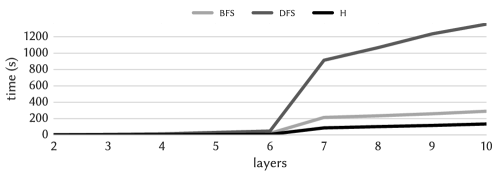
Figure 4. Runtime of the proposed methods with varying the number of layers (DBLP dataset).

The number of computed cores is always larger than the output cores as all methods might compute empty cores or, in the case of dfs, the same core multiple times. Table 2 shows that dfs computes more cores than bfs and h, which conforms to its design principles.

Finally, all methods turn out to be memory-efficient, taking no more than $1.5$GB of memory.

Core-decomposition characterization. Figure 5 reports the distribution of number of cores, core size, and average-degree density (i.e., number of edges divided by number of vertices) of the subgraph corresponding to a core. Distributions are shown by level of the lattice for the SacchCere and Friendfeed datasets. Although the two datasets have very different scales, the distributions exhibit similar trends. Being limited by the number of layers, the number of cores in the first levels of the lattice is very small, but then it exponentially grows until reaching its maximum within the first $25-30\%$ visited levels. The average size of the cores is close to the number of vertices in the first lattice level, when cores’ degree conditions are not very strict. Then it decreases as the number of cores gets larger, with a maximum reached when very small cores stop “propagating” in the lower lattice levels. Finally, the average (average-degree) density tends to increase for higher lattice level. However, there are a couple of exceptions: it decreases ($i$) in the first few levels of SacchCere’s lattice, and ($ii$) in the last levels of both SacchCere and Friendfeed, where the core size starts getting smaller, thus implying small average-degree values.

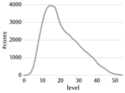
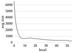
SacchCere
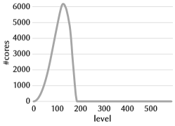
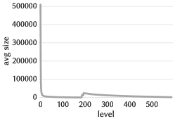
Friendfeed

Figure 5. Distribution of number of cores (left), average core size (center), and average average-degree density of a core (right) to the core-lattice level, for datasets SacchCere (top) and Friendfeed (bottom).

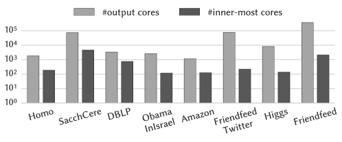
Figure 6. Number of output cores (total and inner-most).

In Figure 6 we show the comparison between the number of all cores and inner-most cores for all the datasets. The number of cores differs quite a lot from dataset to dataset, depending on dataset size, number of layers, and density. The fraction of inner-most cores exhibits a non-decreasing trend as the layers increase, ranging from $0.3\%$ of the total number of output cores (FriendfeedTwitter) to $22\%$ (DBLP).

Given that the inner-most cores are per-se interesting and typically one or more orders of magnitude fewer in number than the total cores, it would be desirable to have a method that effectively exploits the maximality property and extracts the inner-most ones directly, without computing a complete decomposition. This is presented in the next section.

4. Algorithms for Inner-most multilayer cores

In this section we focus on the problem of finding the non-empty inner-most multilayer cores of a multilayer graph (Problem 2). Specifically, the main goal here is to devise a method that is more efficient than a naïve one that computes the whole multilayer core decomposition and then a-posteriori filters non-inner-most cores out. To this end, we devise a recursive algorithm, which is termed im-ml-cores  and whose outline is shown as Algorithm 6 (and Algorithm 7). We provide the details of the algorithm next. In the remainder of this section we assume the layer set $L$ of the input multilayer graph $G=(V,E,L)$ to be an ordered list $[\ell_{1},\ldots,\ell_{|L|}]$. The specific ordering we adopt in this work is by non-decreasing average-degree density, as, among the various orderings tested, this is the one that provides the best experimental results.

The proposed im-ml-cores algorithm is based on the notion of $\ell_{r}$-right-inner-most multilayer cores of a core $C_{\mathbf{k}}$, i.e., all those cores having coreness vector $\mathbf{k^{\prime}}$ equal to $\mathbf{k}$ up to layer $\ell_{r-1}$, and for which the inner-most condition holds for layers from $\ell_{r}$ to $\ell_{|L|}$.

Definition 5 ($\ell_{r}$-right-inner-most multilayer cores).

Given a multilayer graph $G=(V,E,L)$ and a layer $\ell_{r}\in L$, the $\ell_{r}$-right-inner-most multilayer cores of a core $C_{\mathbf{k}}$ of $G$, where $\mathbf{k}=[k_{\ell}]_{\ell\in L}$, correspond to all the cores of $G$ with coreness vector $\mathbf{k^{\prime}}=[k^{\prime}_{\ell}]_{\ell\in L}$ such that $\forall\ell\in[\ell_{1},\ell_{r}):k^{\prime}_{\ell}=k_{\ell}$, and there does not exist any other core with coreness vector  $\mathbf{k}^{\prime\prime}=[k^{\prime\prime}_{\ell}]_{\ell\in L}$ such that $\forall\ell\in[\ell_{1},\ell_{r}):k^{\prime\prime}_{\ell}=k_{\ell}$, $\forall\ell\in[\ell_{r},\ell_{|L|}]:k^{\prime\prime}_{\ell}\geq k^{\prime}_{\ell}$, and $\exists\hat{\ell}\in[\ell_{r},\ell_{|L|}]:k^{\prime\prime}_{\hat{\ell}}>k^{\prime}_{\hat{\ell}}$.

Let $C_{[0]_{|L|}}$ be the root of the core lattice. $C_{[0]_{|L|}}$ has a coreness vector composed of zero components. Therefore, according to the above definition, it is easy to observe that the $\ell_{1}$-right-inner-most multilayer cores of $C_{[0]_{|L|}}$ correspond to the desired ultimate output, i.e., to all inner-most multilayer cores of the input multilayer graph.

Fact 2.

Given a multilayer graph $G=(V,E,L)$, let $\mathbf{I}_{\ell_{1}}$ be the set of all $\ell_{1}$-right-inner-most multilayer cores of core $C_{[0]_{|L|}}$. $\mathbf{I}_{\ell_{1}}$ corresponds to all inner-most multilayer cores of $G$.

The proposed im-ml-cores algorithm recursively computes $\ell_{r}$-right-inner-most multilayer cores, starting from the root of the core lattice (Algorithm 6). The goal is to exploit Fact 2 and ultimately have the $\ell_{1}$-right-inner-most multilayer cores of core $C_{[0]_{|L|}}$ computed. The algorithm makes use of a data structure $\mathcal{M}$ which consists of a sequence of nested maps, one for each layer but the last one (i.e., $\ell_{|L|}$). For every layer $\ell_{r}$ that has been so far processed by the recursive procedure, $\mathcal{M}$ keeps track of the minimum-degree that a core should have in layer $\ell_{r}$ to be recognized as an ineer-most one. Specifically, given a coreness vector $\mathbf{k}$ and a layer $\ell_{r}$, the instruction $\mathcal{M}(\mathbf{k},\ell_{r})$ iteratively accesses the nested maps using the elements of $\mathbf{k}$ up to layer $\ell_{r}$ as keys. As an example, consider a coreness vector $\mathbf{k}=[k_{\ell}]_{\ell\in L}$, with $|L|=3$. $\mathcal{M}(\mathbf{k},\ell_{|L|-1})$ first queries the outer-most map with key $k_{\ell_{1}}$, and obtains a further map. Then, this second map is queried with key $k_{\ell_{2}}$, to finally get the ultimate desired numerical value. Note that, if $\ell_{r}<\ell_{|L|-1}$, then $\mathcal{M}(\mathbf{k},\ell_{r})$ returns a further map. Conversely, if $\ell_{r}=\ell_{|L|-1}$, then $\mathcal{M}(\mathbf{k},\ell_{r})$ returns a numerical value. If $\mathbf{k}$ does not correspond to a sequence of valid keys for $\mathcal{M}$, we assume that $0$ is returned as a default value. $\mathcal{M}$ is initialized as empty, and populated during the various recursive iterations.

Algorithm 6 im-ml-cores

0:  A multilayer graph $G=(V,E,L)$.

0:  The set $\mathbf{I}$ of all inner-most multilayer cores of $G$.

1:  sort $L$ by non-decreasing average-degree density

2:  $\mathcal{M}\leftarrow\emptyset$

3:  $\mathbf{I}\leftarrow$ rim-ml-cores$(G,V,[0]_{|L|},\ell_{1},\mathcal{M})$

Algorithm 7 rim-ml-cores

0:  A multilayer graph $G=(V,E,L)$, a set $S\subseteq V$of vertices, a coreness vector $\mathbf{k}=[k_{\ell}]_{\ell\in L}$, a layer $\ell_{r}\in L$, and a data structure $\mathcal{M}$.

0:  The set $\mathbf{I}_{r}$ of all right-inner-most multilayer cores of $C_{\mathbf{k}}$ given $\ell_{r}$.

1:  $\mathbf{I}_{r}\leftarrow\emptyset$

2:  if $\ell_{r}\neq\ell_{|L|}$ then

3:     $\mathbf{Q}\leftarrow\{\mathbf{k}^{\prime}\mid C_{\mathbf{k}^{\prime}}\in\mbox{$\mathbf{k}$-{coresPath}}(G,S,\mathbf{k},\ell_{r})\}\cup\{\mathbf{k}\}$

4:     $\mathbf{C}\leftarrow\mbox{$\mathbf{k}$-{coresPath}}(G,S,\mathbf{k},\ell_{r})\cup\{S\}$

5:     for all $\mathbf{k^{\prime}}\in\mathbf{Q}$ in decreasing order of $k^{\prime}_{\ell_{r}}$ do

6:        $\mathcal{M}(\mathbf{k^{\prime}},\ell_{r})\leftarrow\emptyset$

7:        $\mathbf{I}_{r}\leftarrow\mathbf{I}_{r}\ \cup$ rim-ml-cores$(G,C_{\mathbf{k^{\prime}}},\mathbf{k^{\prime}},\ell_{r+1},\mathcal{M})$

8:     end for

9:  else

10:     $k_{\mathcal{M}}\leftarrow 0$

11:     for all $\ell\in[\ell_{1},\ell_{|L|})$ do

12:        $\mathbf{k}^{\ell}=[k_{\ell_{1}},\dots,k_{\ell}+1,\dots,k_{\ell_{|L|}}]$

13:        $k_{\mathcal{M}}\leftarrow\max\{k_{\mathcal{M}},\mathcal{M}(\mathbf{k}^{\ell},\ell_{|L|-1})\}$

14:     end for

15:     $\mathbf{k^{\prime}}\leftarrow[k_{\ell_{1}},\dots,k_{\ell_{|L|-1}},k_{\mathcal{M}}]$

16:     $\mathbf{k}^{I}\leftarrow$ Inner-mostCore$(G,S,\mathbf{k^{\prime}},\ell_{|L|})$

17:     if $\mathbf{k}^{I}\neq\textsc{null}$ then

18:        $\mathbf{I}_{r}\leftarrow\mathbf{I}_{r}\cup\mathbf{k}^{I}$

19:        $\mathcal{M}(\mathbf{k}^{I},\ell_{|L|-1})\leftarrow k^{I}_{\ell_{|L|}}+1$

20:     else

21:        $\mathcal{M}(\mathbf{k^{\prime}},\ell_{|L|-1})\leftarrow k^{\prime}_{\ell_{|L|}}$

22:     end if

23:  end if

Figure 7. Execution of the im-ml-cores algorithm (Algorithm 6) on a toy $3$-layer graph.

Figure 8. Content of the $\mathcal{M}$ data structure during the execution of the im-ml-cores algorithm as per the example shown in Fig. 7.

Algorithm 7 may be logically split into two main blocks: the first one (Lines 3 – 8) taking care of the recursion, and the second one (Lines 10 – 22) computing the $\ell_{r}$-right-inner-most cores. The first block of the algorithm is executed when the current $\ell_{r}$ layer is not the last one. In that block the $\mathbf{k}$-coresPath subroutine (already used in Algorithm 3 and described in Section 3.3) is run on set $S$ of vertices, layer $\ell_{r}$, and taking into account the constraints in vector $\mathbf{k}$ (Lines 3 and 4). Then, for each coreness vector $\mathbf{k^{\prime}}$ that has been found, a recursive call is made, where the layer of interest becomes the next layer $\ell_{r+1}$, and the data structure $\mathcal{M}$ is augmented by adding a further (empty) nested map (this new map will be populated within the upcoming recursive executions). The coreness vectors are processed in decreasing order of $k^{\prime}_{\ell_{r}}$. This processing order ensures the correctness of the following: once a multilayer core has been identified as $\ell_{r}$-right-inner-most, it permanently becomes part of the ultimate output cores (no further recursive call will remove it from the output). Note also that, for each $\mathbf{k^{\prime}}$, rim-ml-cores can be run on $C_{\mathbf{k^{\prime}}}$ only, i.e., the core of coreness vector $\mathbf{k^{\prime}}$. This guarantees better efficiency, without affecting correctness.

The second block of the algorithm (Lines 10 – 22) works as follows. When the last layer has been reached, i.e., $\ell_{r}=\ell_{|L|}$, the current recursion ends, and an $\ell_{r}$-right-inner-most multilayer core is returned (if any). First of all, the algorithm computes a coreness vector $\mathbf{k^{\prime}}$ which is potentially $\ell_{r}$-right-inner-most (Lines 10 – 15). In this regard, note that the $k_{\mathcal{M}}$ value is derived from the information that has been stored in $\mathcal{M}$ in the earlier recursive iterations. Finally, the algorithm computes the inner-most core in $\ell_{|L|}$ constrained by $\mathbf{k^{\prime}}$, by means of the Inner-mostCore subroutine. Such a subroutine, similarly to the $\mathbf{k}$-coresPath one, takes as input a multilayer graph $G$, a subset $S$ of vertices, a coreness vector $\mathbf{k}$, and a layer $\ell$. It returns the multilayer core having coreness vector of highest $\ell$-th component of the vertices in $S$, considering the constraints specified in $\mathbf{k}$. If the Inner-mostCore procedure actually returns a multilayer core, then it is guaranteed that such a core is $\ell_{r}$-right-inner-most, and is therefore added to the solution (and $\mathcal{M}$ is updated accordingly).

In Figure 7 we show an example of the execution of the proposed im-ml-cores algorithm for a simple 3-layer graph, while Figure 8 reports the content of the $\mathcal{M}$ data structure for this example. Every box corresponds to a call of Algorithm 7, for which we specify ($i$) the input parameters ($G$ and $\mathcal{M}$ are omitted for the sake of brevity), ($ii$) the calls to the $\mathbf{k}$-coresPath or Inner-mostCore subroutines, and ($iii$) the content of $\mathbf{Q}$ (when it is instantiated). For instance, the coreness vector given as input to Inner-mostCore at box $1.3.4$ has the last element equal to the maximum between what is stored in $\mathcal{M}$ at the end of the paths $1\rightarrow 0$ and $\ 0\rightarrow 1$, i.e., $8$ and $5$, that have been set at boxes $1.2.3$ and $1.3.3$, respectively.

4.1. Experimental results

Running times. We asses the efficiency of im-ml-cores (for short im) by comparing it to the aforementioned naïve approach for computing inner-most multilayer cores, which consists in firstly computing all multilayer cores (by means of one of the three algorithms presented in Section 3) and filtering out the non-inner-most ones. The results of this experiment are reported in Table 3. First of all, it can be observed that the a-posteriori filtering of the inner-most multilayer cores does not consistently affect the runtime of the algorithms for multilayer core decomposition: this means that most of the time is spent for computing the overall core decomposition. The main outcome of this experiment is that the running time of the proposed im method is smaller than the time required by bfs, dfs, or h summed up to the time spent in the a-posteriori filtering, with considerable speed-up from $1.3$ to an order of magnitude on the larger datasets, e.g., FriendfeedTwitter and Friendfeed. The only exception is on the DBLP dataset where bfs and h run slightly faster, probably due to fact that its edges are (almost) equally distributed among the layers, which makes the effectiveness of the ordering vanish.

Table 3. Runtime (in seconds) of the methods for multilayer core decomposition, the a-posteriori filtering of the inner-most multilayer cores, and the proposed im-ml-cores method for directly computing inner-most multilayer cores.

dataset	bfs	dfs	h	filtering	im
Homo	$13$	$27$	$12$	$0.5$	$5$
SacchCere	$1\,134$	$2\,627$	$1\,146$	$24$	$336$
DBLP	$68$	$282$	$29$	$1$	$148$
ObamaInIsrael	$226$	$150$	$177$	$7$	$120$
Amazon	$3\,981$	$5\,278$	$3\,913$	$129$	$2\,530$
FriendfeedTwitter	$61\,113$	$1\,973$	$59\,520$	$276$	$1\,583$
Higgs	$2\,480$	$640$	$2\,169$	$33$	$356$
Friendfeed	$58\,278$	$13\,356$	$47\,179$	$394$	$2\,640$

Characterization. We also show the characteristics of the inner-most multilayer cores. Figure 9 reports the distribution of number, size, and average-degree density of all cores and inner-most cores only. Distributions are shown in a way similar to what previously done in Figure 5, i.e., by level of the core lattice, and for the SacchCere and Amazon datasets.

For both datasets, there are no inner-most cores in the first levels of the lattice. As expected, the number of inner-most cores considerably increases when the number of all cores decreases. This is due to the fact that some cores stop propagating throughout the lattice, hence they are recognized as inner-most. In general, inner-most cores are on average smaller than all multilayer cores. Nonetheless, for the levels 12 and 13 of the Amazon dataset, inner-most cores have greater size than all cores. This behavior is consistent with our definitions: inner-most cores are cores without descendants, thus they are expected to be the smallest-sized ones, but they do not necessarily have to. Finally, the distribution of the average-degree density exhibits a similar trend to the distribution of the size: this is expected as the two measures depend on each other.

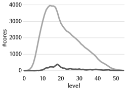
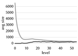
SacchCere
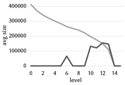
Amazon

Figure 9. Comparison of the distributions, to the core-lattice level, of number (left), average size (center), and average average-degree density (right) of multilayer cores and inner-most multilayer cores, for datasets SacchCere (top) and Amazon (bottom).

5. Multilayer densest subgraph

In this section we showcase the usefulness of multilayer core-decomposition in the context of multilayer densest-subgraph discovery. Particularly, we show how to exploit the multilayer core-decomposition to devise an algorithm with approximation guarantees for the Multilayer Densest Subgraph problem introduced in Section 2 (Problem 3), thus extending to the multilayer setting the intuition at the basis of the well-known $\frac{1}{2}$-approximation algorithm (Asahiro et al., 2000; Charikar, 2000) for single-layer densest-subgraph extraction.

5.1. Hardness

We start by formally showing that the Multilayer Densest Subgraph problem (Problem 3) is $\mathbf{NP}$-hard.

Theorem 3.

Problem 3 is $\mathbf{NP}$-hard.

To prove the theorem, we introduce two variants of Problem 3’s objective function, i.e., $\delta_{\textsc{all}}(\cdot)$, which considers all layers in $L$, and $\delta_{\textsc{$\neg$all}}(\cdot)$, which considers all subsets of layers but the whole layer set $L$. Specifically, for any given multilayer graph $G=(V,E,L)$ and vertex subset $S\subseteq V$, the two functions are defined as:

(3) $$\delta_{\textsc{all}}(S)=\min_{\ell\in L}\frac{|E_{\ell}[S]|}{|S|}|L|^{\beta},$$

(4) $$\delta_{\textsc{$\neg$all}}(S)=\max_{\hat{L}\in 2^{L}\setminus\{L\}}\min_{\ell\in\hat{L}}\frac{|E_{\ell}[S]|}{|S|}|\hat{L}|^{\beta}.$$

We also define $deg_{max}$ as the maximum degree of a vertex in a layer:

(5) $$deg_{max}=\max_{\ell\in L}\max_{u\in V}deg(u,\ell),$$

and introduce the following three auxiliary lemmas.

Lemma 1.

$\delta_{\textsc{all}}(S)\geq\frac{1}{|V|}|L|^{\beta}$, for all $S\subseteq V$ such that $\forall\ell\in L:|E_{\ell}[S]|>0$.

Proof.

For a vertex set $S$ spanning at least one edge in every layer, it holds that $\min_{\ell\in L}\frac{|E_{\ell}[S]|}{|S|}\geq\frac{1}{|V|}$, and, therefore, $\delta_{\textsc{all}}(S)=\min_{\ell\in L}\frac{|E_{\ell}[S]|}{|S|}|L|^{\beta}\geq\frac{1}{|V|}|L|^{\beta}$. ∎

Lemma 2.

$\delta_{\textsc{$\neg$all}}(S)\leq\frac{deg_{max}}{2}(|L|-1)^{\beta}$, for all $S\subseteq V$.

Proof.

The maximum density of a vertex set $S$ in a layer can be at most equal to the density of the maximum clique, i.e., at most $\frac{(deg_{max}+1)~{}deg_{max}}{2~{}(deg_{max}+1)}=\frac{deg_{max}}{2}$. At the same time, the size of a layer set $\hat{L}$ in the function $\delta_{\textsc{$\neg$all}}(\cdot)$ can be at most $|L|-1$ (as the whole layer set $L$ is not considered in $\delta_{\textsc{$\neg$all}}(\cdot)$). This means that $\delta_{\textsc{$\neg$all}}(S)=\max_{\hat{L}\in 2^{L}\setminus\{L\}}\min_{\ell\in\hat{L}}\frac{|E_{\ell}[S]|}{|S|}|\hat{L}|^{\beta}\leq\frac{deg_{max}}{2}(|L|-1)^{\beta}$. ∎

Lemma 3.

β¿ log—L—-1(—V—2$deg_{max}$)×log—L—(—L— -1)1 - log—L—(—L— - 1)   ⇔  1—V——L—^β¿ $deg_{max}$2(—L— - 1)^β.

Proof.

$$\beta\ >\ \frac{\log_{|L|-1}\left(\frac{|V|}{2}deg_{max}\right)\times\log_{|L|}(|L|-1)}{1-\log_{|L|}(|L|-1)}$$

$$\Leftrightarrow \left(1-\log_{|L|}(|L|-1)\right)\beta\ >\ \log_{|L|-1}\left({\textstyle\frac{|V|}{2}}deg_{max}\right)\times\log_{|L|}(|L|-1)$$

$$\Leftrightarrow \beta\ >\ \log_{|L|-1}\left({\textstyle\frac{|V|}{2}}deg_{max}\right)\times\log_{|L|}(|L|-1)+\beta\log_{|L|}(|L|-1)$$

$$\Leftrightarrow \frac{\beta}{\log_{|L|}(|L|-1)}\ >\ \log_{|L|-1}\left({\textstyle\frac{|V|}{2}}deg_{max}\right)+\beta$$

$$\Leftrightarrow \frac{\log_{|L|}|L|^{\beta}}{\log_{|L|}(|L|-1)}\ >\ \log_{|L|-1}\left({\textstyle\frac{|V|}{2}}deg_{max}\right)+\log_{|L|-1}(|L|-1)^{\beta}$$

$$\Leftrightarrow \log_{|L|-1}|L|^{\beta}\ >\ \log_{|L|-1}\left({\textstyle\frac{|V|}{2}}deg_{max}(|L|-1)^{\beta}\right)$$

$$\Leftrightarrow |L|^{\beta}\ >\ {\textstyle\frac{|V|}{2}}deg_{max}(|L|-1)^{\beta}$$

$$\Leftrightarrow \frac{1}{|V|}|L|^{\beta}\ >\ \frac{deg_{max}}{2}(|L|-1)^{\beta}.$$

∎

With Lemmas 1–3 in place, we are now ready to provide the ultimate proof of Theorem 3.

Proof.

We reduce from the Min-Avg Densest Common Subgraph (DCS-MA) problem (Jethava and Beerenwinkel, 2015), which aims at finding a subset of vertices $S\subseteq V$ from a multilayer graph $G=(V,L,S)$ maximizing $\min_{\ell\in L}\frac{E_{\ell}[S]}{|S|}$, and has been recently shown to be $\mathbf{NP}$-hard in (Charikar et al., 2018). We distinguish two cases. The first (trivial) one is when $G$ has a layer with no edges. In this case any vertex subset would be an optimal solution for DCS-MA (with overall objective function equal to zero), including the optimal solution to our Multilayer Densest Subgraph problem run on the same $G$ (no matter which $\beta$ is used). In the second case $G$ has at least one edge in every layer. In this case solving our Multilayer Densest Subgraph problem on $G$, with $\beta$ set to any value $>\frac{\log_{|L|-1}\left(\frac{|V|}{2}deg_{max}\right)\times\log_{|L|}(|L|-1)}{1-\log_{|L|}(|L|-1)}$, gives a solution that is optimal for DCS-MA as well. Indeed, it can be observed that, for all $S\subseteq V$ such that $\forall\ell\in L:|E_{\ell}[S]|>0$:

$$\delta_{\textsc{all}}(S) \geq \frac{1}{|V|}|L|^{\beta}\qquad\qquad\qquad\{\mbox{Lemma~{}\ref{lemma:densesthard1}}\}$$

$$> \frac{deg_{max}}{2}(|L|-1)^{\beta}~{}\qquad\{\mbox{Lemma~{}\ref{lemma:densesthard3}}\}$$

$$\geq \delta_{\textsc{$\neg$all}}(S).\qquad\qquad\qquad\{\mbox{Lemma~{}\ref{lemma:densesthard2}}\}$$

This means that, for that particular value of $\beta$, the optimal solution of Multilayer Densest Subgraph on input $G$ is given by maximizing the $\delta_{\textsc{all}}(\cdot)$ function, which considers all layers and is, as such, equivalent to the objective function underlying the DCS-MA problem. This completes the proof. ∎

5.2. Algorithms

The approximation algorithm we devise for the Multilayer Densest Subgraph problem is very simple: it computes the multilayer core decomposition of the input graph, and, among all cores, takes the one maximizing the objective function $\delta$ as the output densest subgraph (Algorithm 8). Despite its simplicity, the algorithm achieves provable approximation guarantees proportional to the number of layers of the input graph, precisely equal to $\frac{1}{2|L|^{\beta}}$. We next formally prove this result.

Algorithm 8 ml-densest

0:  A multilayer graph $G=(V,E,L)$ and a real number $\beta\in\mathbb{R}^{+}$.

0:  $C^{*}\subseteq V$.

1:  $\mathbf{C}\leftarrow\mbox{{MultiLayerCoreDecomposition}}(G)$# Any of Algorithms 2, 3, 5 can be used

2:  $C^{*}\leftarrow\arg\max_{C\in\mathbf{C}}\delta(C)$# Equation (1)

Let $\mathbf{C}$ be the core decomposition of the input multilayer graph $G=(V,E,L)$ and $C^{*}$ denote the core in $\mathbf{C}$ maximizing the density function $\delta$, i.e., $C^{*}=\arg\max_{C\in\mathbf{C}}\delta(C)$. Then, $C^{*}$ corresponds to the subgraph output by the proposed ml-densest algorithm. Let also $C^{(\mu)}$ denote the subgraph maximizing the minimum degree in a single layer, i.e., $C^{(\mu)}=\arg\max_{S\subseteq V}f(S)$, where $f(S)=\max_{\ell\in L}\mu(S,\ell)$, while $\ell^{(\mu)}=\arg\max_{\ell\in L}\mu(C^{(\mu)},\ell)$. It is easy to see that $C^{(\mu)}\in\mathbf{C}$. Finally, let $S^{*}_{\mbox{{sl}}}$ be the densest subgraph among all single-layer densest subgraphs, i.e., $S^{*}_{\mbox{{sl}}}=\arg\max_{S\subseteq V}g(S)$, where $g(S)=\max_{\ell\in L}\frac{|E_{\ell}[S]|}{|S|}$, and $\ell^{*}$ be the layer where $S^{*}_{\mbox{{sl}}}$ exhibits its largest density, i.e., $\ell^{*}=\arg\max_{\ell\in L}\frac{|E_{\ell}[S^{*}_{\mbox{{sl}}}]|}{|S^{*}_{\mbox{{sl}}}|}$. We start by introducing the following two lemmas that can straightforwardly be derived from the definitions of $C^{*}$, $C^{(\mu)}$, $S^{*}_{\mbox{{sl}}}$, $\ell^{(\mu)}$, and $\ell^{*}$:

Lemma 4.

$\delta(C^{*})\geq\delta(C^{(\mu)})$.

Proof.

By definition, $C^{(\mu)}$ is a multilayer core described by (among others) the coreness vector  $\mathbf{k}=[k_{\ell}]_{\ell\in L}$ with $k_{\ell^{(\mu)}}=\max_{\ell\in L}\mu(C^{(\mu)},\ell)$, and $k_{\ell}=0$, $\forall\ell\neq\ell^{(\mu)}$. Then $C^{(\mu)}\in\mathcal{C}$. As $C^{*}=\arg\max_{C\in\mathcal{C}}\delta(C)$, it holds that $\delta(C^{*})\geq\delta(C^{(\mu)})$. ∎

Lemma 5.

$\delta(S^{*})\leq\frac{\textstyle|E_{\ell^{*}}[S^{*}_{\mbox{{sl}}}]|}{\textstyle|S^{*}_{\mbox{{sl}}}|}|L|^{\beta}$.

Proof.

$$\!\!\!\!\delta(S^{*}) \!\!=\!\! \max_{\hat{L}\subseteq L}\min_{\ell\in\hat{L}}\frac{|E_{\ell}[S^{*}]|}{|S^{*}|}|\hat{L}|^{\beta}\ \leq\ \max_{\ell\in L}\frac{|E_{\ell}[S^{*}]|}{|S^{*}|}|L|^{\beta}\ \leq\ \frac{|E_{\ell^{*}}[S^{*}_{\mbox{{sl}}}]|}{|S^{*}_{\mbox{{sl}}}|}|L|^{\beta}.$$

∎

The following further lemma shows a lower bound on the minimum degree of a vertex in $S^{*}_{\mbox{{sl}}}$:

Lemma 6.

$\mu(S^{*}_{\mbox{{sl}}},\ell^{*})\geq\frac{\textstyle|E_{\ell^{*}}[S^{*}_{\mbox{{sl}}}]|}{\textstyle|S^{*}_{\mbox{{sl}}}|}$.

Proof.

As $S^{*}_{\mbox{{sl}}}$ is the subgraph maximizing the density in layer $\ell^{*}$, removing the minimum-degree node from $S^{*}_{\mbox{{sl}}}$ cannot increase that density. Thus, it holds that:

$$\frac{|E_{\ell^{*}}[S^{*}_{\mbox{{sl}}}]|}{|S^{*}|}\geq\frac{|E_{\ell^{*}}[S^{*}_{\mbox{{sl}}}]|-\mu(S^{*}_{\mbox{{sl}}},\ell^{*})}{|S^{*}_{\mbox{{sl}}}|-1}$$

$$\Leftrightarrow \mu(S^{*}_{\mbox{{sl}}},\ell^{*})\geq|E_{\ell^{*}}[S^{*}_{\mbox{{sl}}}]|\frac{|S^{*}_{\mbox{{sl}}}|-1}{|S^{*}_{\mbox{{sl}}}|}-|E_{\ell^{*}}[S^{*}_{\mbox{{sl}}}]|\qquad$$

$$\Leftrightarrow \mu(S^{*}_{\mbox{{sl}}},\ell^{*})\geq\frac{|E_{\ell^{*}}[S^{*}_{\mbox{{sl}}}]|}{|S^{*}_{\mbox{{sl}}}|}.\qquad\qquad\qquad\qquad\qquad$$

∎

The approximation factor of the proposed ml-densest algorithm is ultimately stated in the next theorem:

Theorem 4.

$\delta(C^{*})\geq\frac{\textstyle 1}{\textstyle 2|L|^{\beta}}\delta(S^{*})$.

Proof.

$$\!\delta(C^{*})\!\!\!\! \geq \delta(C^{(\mu)})\qquad\qquad\qquad\qquad\qquad\qquad\qquad\quad\{\mbox{Lemma~{}\ref{lemma:SLinnermost}}\}$$

$$\geq \max_{\ell\in L}\frac{|E_{\ell}[C^{(\mu)}]|}{|C^{(\mu)}|}1^{\beta}=\max_{\ell\in L}\frac{|E_{\ell}[C^{(\mu)}]|}{|C^{(\mu)}|}\qquad\{\mbox{Equation~{}(\ref{eq:densestfunction})}\}$$

$$\geq \frac{1}{2}\max_{\ell\in L}\mu(C^{(\mu)},\ell)\qquad\qquad\{\mbox{as avg degree $\geq$ min degree}\}$$

$$= \frac{1}{2}\mu(C^{(\mu)},\ell^{(\mu)})\qquad\qquad\qquad\qquad\{\mbox{by definition of $C^{(\mu)}$}\}$$

$$\geq \frac{1}{2}\mu(S^{*}_{\mbox{{sl}}},\ell^{*})\qquad\quad\{\mbox{optimality of $C^{(\mu)}$\ w.r.t. min degree}\}$$

$$\geq \frac{1}{2}\frac{|E_{\ell^{*}}[S^{*}_{\mbox{{sl}}}]|}{|S^{*}_{\mbox{{sl}}}|}\qquad\qquad\qquad\qquad\qquad\qquad\quad\ \{\mbox{Lemma~{}\ref{lemma:LBdensestmindeg}}\}$$

$$\geq \frac{1}{2|L|^{\beta}}\delta(S^{*}).\qquad\qquad\qquad\qquad\qquad\qquad\quad\ \{\mbox{Lemma~{}\ref{lemma:SLdensest}}\}$$

∎

The following corollary shows that the theoretical approximation guarantee stated in Theorem 4 remains the same even if only the inner-most cores are considered (although, clearly, considering the whole core decomposition may lead to better accuracy in practice).

Corollary 4.

Given a multilayer graph $G=(V,E,L)$, let $\mathbf{C}_{\textsc{im}}$ be the set of all inner-most multilayer cores of $G$, and let $C^{*}_{\textsc{im}}=\arg\max_{C\in\mathbf{C}_{\textsc{im}}}\delta(C)$. It holds that $\delta(C_{\textsc{im}}^{*})\geq\frac{1}{2|L|^{\beta}}\delta(S^{*})$.

Proof.

Let $C^{(\mu)}_{\textsc{im}}\in\mathbf{C}_{\textsc{im}}$ be an inner-most core of $G$ whose coreness vector has a component equal to $\ell^{(\mu)}$. It is easy to see that the result in Lemma 4 holds for $C^{*}_{\textsc{im}}$ and $C^{(\mu)}_{\textsc{im}}$ too, i.e., becoming $\delta(C^{*}_{\textsc{im}})\geq\delta(C^{(\mu)}_{\textsc{im}})$, while the proof of Theorem 4 holds as is, by simply replacing $C^{*}$ with $C^{*}_{\textsc{im}}$ and $C^{(\mu)}$ with $C^{(\mu)}_{\textsc{im}}$. ∎

Finally, we observe that the result in Theorem 4 carries over to the Min-Avg Densest Common Subgraph (DCS-MA) problem studied in (Charikar et al., 2018; Jethava and Beerenwinkel, 2015; Reinthal et al., 2016; Semertzidis et al., 2019) as well, as that problem can be reduced to our Multilayer Densest Subgraph problem (as shown in Theorem 3).

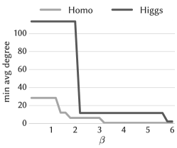
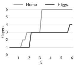
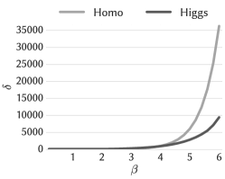
Figure 10. Multilayer densest-subgraph extraction (Homo and Higgs datasets): minimum average-degree density in a layer, number of selected layers, size, and objective-function value $\delta$ of the output densest subgraphs with varying $\beta$.

5.3. Experimental results

We experimentally evaluate our ml-densest algorithm (Algorithm 8) on the datasets in Table 1. Figure 10 reports the results – minimum average-degree density in a layer, number of selected layers, size, objective-function value $\delta$ – on the Homo and Higgs datasets, with varying $\beta$. The remaining datasets, which we omit due to space constraints, exhibit similar trends on all measures.

The trends observed in the figure conform to what expected: the smaller $\beta$, the more the objective function privileges solutions with large average-degree density in a few layers (or even just one layer, for $\beta$ close to zero). The situation is overturned with larger values of $\beta$, where the minimum average-degree density drops significantly, while the number of selected layers stands at $6$ for Homo and $4$ for Higgs. In-between $\beta$ values lead to a balancing of the two terms of the objective function, thus giving more interesting solutions. Also, by definition, $\delta$ as a function of $\beta$ draws exponential curves.

Finally, as anecdotal evidence of the output of Algorithm 8, in Figure 11 we report the densest subgraph extracted from DBLP. The subgraph contains 10 vertices and $5$ layers automatically selected by the objective function $\delta$. The minimum average-degree density is encountered on the layers corresponding to topics “graph” and “algorithm” (green and yellow layers in the figure), and is equal to $1.2$. The objective-function value is $\delta=41.39$. Note that the subgraph is composed of two connected components. In fact, like the single-layer case, multilayer cores are not necessarily connected.

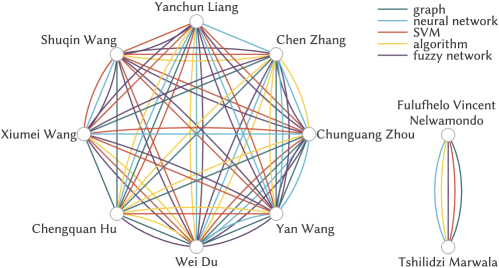
Figure 11. Multilayer densest subgraph extracted by Algorithm 8 from the DBLP dataset ($\beta=2.2$).

6. Multilayer quasi-cliques

Another interesting insight into the notion of multilayer cores is about their relationship with (quasi-)cliques. In single-layer graphs it is well-known that cores can be exploited to speed-up the problem of finding cliques, as a clique of size $k$ is guaranteed to be contained into the $(k-1)$-core. Interestingly, a similar relationship holds in the multilayer context too. Given a multilayer graph $G=(V,E,L)$, a layer $\ell\in L$, and a real number $\gamma\in(0,1]$, a subgraph $G[S]=(S\subseteq V,E[S],L)$ of $G$ is said to be a $\gamma$-quasi-clique in layer $\ell$ if all its vertices have at least $\gamma(|S|-1)$ neighbors in layer $\ell$ within $S$, i.e., $\forall u\in S:deg_{S}(u,\ell)\geq\gamma(|S|-1)$. Jiang et al. (Jiang and Pei, 2009) study the problem of extracting frequent cross-graph quasi-cliques: given a multilayer graph $G=(V,E,L)$, a function $\Gamma:L\rightarrow(0,1]$ assigning a real value to every layer in $L$, a real number $\mbox{\emph{min\_sup}}\in(0,1]$, and an integer $\mbox{\emph{min\_size}}>1$, find all maximal subgraphs $G[S]$ of $G$ of size larger than min_size such that there exist at least $\mbox{\emph{min\_sup}}\times|L|$ layers $\ell$ for which $G[S]$ is a $\Gamma(\ell)$-quasi-clique.

The following theorem shows that a frequent cross-graph quasi-clique of size $\geq\!\mbox{\emph{min\_size}}$ is necessarily contained into a $\mathbf{k}$-core described by a coreness vector $\mathbf{k}=[k_{\ell}]_{\ell\in L}$ such that there exists a fraction of min_sup layers $\ell$ where $k_{\ell}=\lceil\Gamma(\ell)(\mbox{\emph{min\_size}}-1)\rceil$.

Theorem 5.

Given a multilayer graph $G=(V,E,L)$, a real-valued function $\Gamma:L\rightarrow(0,1]$, a real number $\mbox{\emph{min\_sup}}\in(0,1]$, and an integer $\mbox{\emph{min\_size}}>1$, a frequent cross-graph quasi-clique of $G$ complying with parameters $\Gamma$, min_sup, and min_size is contained into a $\mathbf{k}$-core with coreness vector $\mathbf{k}=[k_{\ell}]_{\ell\in L}$ such that $|\{\ell\in L:k_{\ell}=\lceil\Gamma(\ell)(\mbox{\emph{min\_size}}-1)\rceil\}|=\lceil\mbox{\emph{min\_sup}}\times|L|\rceil$.

Proof.

Assume that a cross-graph quasi-clique $S$ of $G$ complying with parameters $\Gamma$, min_sup, and min_size is not contained into any $\mathbf{k}$-core with coreness vector $\mathbf{k}=[k_{\ell}]_{\ell\in L}$ such that $|\{\ell\in L:k_{\ell}=\lceil\Gamma(\ell)(\mbox{\emph{min\_size}}-1)\rceil\}|=\lceil\mbox{\emph{min\_sup}}\times|L|\rceil$. This means that $S$ contains a vertex $u$ such that $|\{\ell\in L:deg_{S}(u,\ell)\geq\Gamma(\ell)(\mbox{\emph{min\_size}}-1)\}|<\mbox{\emph{min\_sup}}\times|L|$, which means that $|\{\ell\in L:deg_{S}(u,\ell)\geq\Gamma(\ell)(|S|-1)\}|<\mbox{\emph{min\_sup}}\times|L|$ as well, since $|S|\geq\mbox{\emph{min\_size}}$. This violates the definition of frequent cross-graph quasi-clique. ∎

As a simple corollary, the computation of frequent cross-graph quasi-cliques can therefore be circumstantiated to the subgraph given by the union of all multilayer cores complying with the condition stated in Theorem 5.

Corollary 5.

Given a multilayer graph $G=(V,E,L)$, a real-valued function $\Gamma:L\rightarrow(0,1]$, a real number $\mbox{\emph{min\_sup}}\in(0,1]$, and an integer $\mbox{\emph{min\_size}}>1$, let $G^{\prime}=(V^{\prime},E^{\prime},L)$ the subgraph of $G$ given by the union of all multilayer cores of $G$ complying with Theorem 5. It holds that all cross-graph quasi-cliques of $G$ complying with parameters $\Gamma$, min_sup, and min_size are contained into $G^{\prime}$.

The finding in Corollary 5 can profitably be exploited to have a more efficient extraction of frequent cross-graph quasi-cliques. Specifically, the idea is to ($i$) compute all multilayer cores of the input graph $G$ (including the non-distinct ones, as the condition stated in Theorem 5 refers to not necessarily maximal coreness vectors); ($ii$) process all multilayer cores of $G$ one by one, retain only the ones complying with Theorem 5, and compute the subgraph $G^{\prime}$ induced by the union of all such cores; ($iii$) run any algorithm for frequent cross-graph quasi-cliques on $G^{\prime}$. Based on the above theoretical results, such a procedure is guaranteed to be sound and complete, and it is expected to provide a significant speed-up, as $G^{\prime}$ is expected to be much smaller than the original graph $G$.

Table 4. Comparison of the runtime of the efficient extraction of frequent cross-graph quasi-cliques by Corollary 5 and of the original algorithm (Jiang and Pei, 2009), for the SacchCere dataset. The evaluation is proposed varying one of the parameters, i.e., $\Gamma$, min_sup, and min_size, at a time. The number of solution quasi-cliques and the number of vertices $|V^{\prime}|$ of the subgraph $G^{\prime}$ are also reported. For each run of the experiment, the smallest runtime is bolded.

# solution runtime (s) $\Gamma$ min_sup min_size quasi-cliques $|V^{\prime}|$ Corollary 5 (Jiang and Pei, 2009) $1$ $1$ $1$ $1$ $.2$ $.2$ $1$ $0.5$ $6$ $2$ $371$ $\mathbf{3}$ $169$ $.9$ $.9$ $.9$ $.9$ $.2$ $.2$ $.9$ $2$ $371$ $\mathbf{25}$ $17\,561$ $.8$ $.8$ $.8$ $.8$ $.2$ $.2$ $.8$ $6$ $1\,196$ $\mathbf{734}$ $22\,932$ $.7$ $.7$ $.7$ $.7$ $.2$ $.2$ $.7$ $6$ $1\,196$ $\mathbf{728}$ $23\,376$ $.6$ $.6$ $.6$ $.6$ $.2$ $.2$ $.6$ $59$ $2\,300$ $\mathbf{5\,200}$ $28\,948$ $.5$ $.5$ $.5$ $.5$ $.2$ $.2$ $.5$ $59$ $2\,300$ $\mathbf{5\,123}$ $29\,677$

# solution runtime (s) $\Gamma$ min_sup min_size quasi-cliques $|V^{\prime}|$ Corollary 5 (Jiang and Pei, 2009) $.5$ $.5$ $.5$ $.5$ $.2$ $.2$ $.5$ $1$ $3$ $2$ $152$ $\mathbf{2}$ $281$ $0.9$ $2$ $152$ $\mathbf{2}$ $282$ $0.8$ $28$ $940$ $\mathbf{23}$ $292$ $0.7$ $323$ $3\,271$ $\mathbf{205}$ $411$ $0.6$ $323$ $3\,271$ $\mathbf{203}$ $414$ $0.5$ $1\,630$ $4\,581$ $\mathbf{2\,569}$ $3\,075$

# solution runtime (s) $\Gamma$ min_sup min_size quasi-cliques $|V^{\prime}|$ Corollary 5 (Jiang and Pei, 2009) $.5$ $.5$ $.5$ $.5$ $.2$ $.2$ $.5$ $0.5$ $7$ $27$ $2\,254$ $\mathbf{5\,606}$ $34\,904$ $6$ $59$ $2\,300$ $\mathbf{5\,123}$ $29\,677$ $5$ $357$ $3\,363$ $\mathbf{4\,493}$ $21\,206$ $4$ $378$ $3\,363$ $\mathbf{3\,704}$ $15\,465$ $3$ $1\,630$ $4\,581$ $\mathbf{2\,569}$ $3\,075$

Table 5. Comparison of the runtime of the efficient extraction of frequent cross-graph quasi-cliques by Corollary 5 and of the original algorithm (Jiang and Pei, 2009), for the DBLP dataset. The evaluation is proposed varying one of the parameters, i.e., $\Gamma$, min_sup, and min_size, at a time. The number of solution quasi-cliques and the number of vertices $|V^{\prime}|$ of the subgraph $G^{\prime}$ are also reported. $++$ indicates runtime longer than $259\,200$ seconds (i.e., $3$ days). For each run of the experiment, the smallest runtime is bolded.

# solution runtime (s) $\Gamma$ min_sup min_size quasi-cliques $|V^{\prime}|$ Corollary 5 (Jiang and Pei, 2009) $1$ $1$ $1$ $1$ $1$ $1$ $1$ $1$ $1$ $1$ $0.2$ $8$ $2$ $18$ $\mathbf{0.2}$ $26\,496$ $.9$ $.9$ $.9$ $.9$ $.9$ $.9$ $.9$ $.9$ $.9$ $.9$ $2$ $18$ $\mathbf{0.2}$ $26\,112$ $.8$ $.8$ $.8$ $.8$ $.8$ $.8$ $.8$ $.8$ $.8$ $.8$ $13$ $75$ $\mathbf{0.3}$ $26\,867$ $.7$ $.7$ $.7$ $.7$ $.7$ $.7$ $.7$ $.7$ $.7$ $.7$ $18$ $196$ $\mathbf{1}$ $27\,387$ $.6$ $.6$ $.6$ $.6$ $.6$ $.6$ $.6$ $.6$ $.6$ $.6$ $18$ $196$ $\mathbf{1}$ $27\,084$ $.5$ $.5$ $.5$ $.5$ $.5$ $.5$ $.5$ $.5$ $.5$ $.5$ $121$ $801$ $\mathbf{18}$ $31\,508$

# solution runtime (s) $\Gamma$ min_sup min_size quasi-cliques $|V^{\prime}|$ Corollary 5 (Jiang and Pei, 2009) $.5$ $.5$ $.5$ $.5$ $.5$ $.5$ $.5$ $.5$ $.5$ $.5$ $0.5$ $3$ $8$ $182$ $\mathbf{0.2}$ $26\,969$ $0.4$ $195$ $2\,375$ $\mathbf{1}$ $26\,964$ $0.3$ $3\,394$ $22\,659$ $\mathbf{210}$ $32\,981$

# solution runtime (s) $\Gamma$ min_sup min_size quasi-cliques $|V^{\prime}|$ Corollary 5 (Jiang and Pei, 2009) $.5$ $.5$ $.5$ $.5$ $.5$ $.5$ $.5$ $.5$ $.5$ $.5$ $0.2$ $13$ $1$ $75$ $\mathbf{0.2}$ $26\,644$ $12$ $1$ $75$ $\mathbf{0.2}$ $27\,136$ $11$ $8$ $196$ $\mathbf{0.7}$ $26\,966$ $10$ $10$ $196$ $\mathbf{0.7}$ $27\,116$ $9$ $116$ $801$ $\mathbf{18}$ $32\,372$ $8$ $121$ $801$ $\mathbf{18}$ $31\,508$ $7$ $1\,292$ $3\,468$ $\mathbf{181}$ $113\,558$ $6$ $1\,370$ $3\,468$ $\mathbf{198}$ $113\,520$ $5$ $7\,599$ $15\,316$ $\mathbf{3\,790}$ $++$ $4$ $8\,578$ $15\,316$ $\mathbf{3\,502}$ $++$

6.1. Experimental results

We show in Tables 4 and 5 the experimental results about the comparison of the algorithm proposed by Jiang et al. (Jiang and Pei, 2009) and the more efficient extraction of frequent cross-graph quasi-cliques by Corollary 5. Table 4 refers to the SacchCere dataset, while Table 5 to the DBLP dataset. To evaluate the effect of the parameters, i.e., the function $\Gamma$, min_sup, and min_size, on the performance of the two approaches, we vary a parameter at a time keeping the other two fixed. With regards to the values selected for $\Gamma$, we fix $\Gamma(\ell_{5})=\Gamma(\ell_{6})=0.2$ in all the experiments involving the SacchCere dataset, due to the imbalance of the distribution of the edges in favor of the other five layers (i.e., layers $\ell_{1},\ldots,\ell_{4},\ell_{7}$). Instead, given the uniformity of the edge density across the layers of the DBLP dataset, $\Gamma$ is modified coherently for all the layer in this latter case. In addition to the execution times, for each configuration of the parameters, we also report the number of solution frequent cross-graph quasi-cliques and the number of vertices $|V^{\prime}|$ of the subgraph $G^{\prime}$ identified by Corollary 5.

The first thing to notice is that, in both datasets and for every configuration, our approach is faster than the algorithm by Jiang et al. (Jiang and Pei, 2009). The actual speed-up varies with the size of $|V^{\prime}|$ (with respect to $|V|$) which, in turn, is affected by the mining parameters. For the SacchCere dataset, we obtain the most extreme cases when varying min_sup (middle table): our approach is able to prune from 30% ($\mbox{\emph{min\_sup}}=0.5$) up to 98% ($\mbox{\emph{min\_sup}}=1$) of the input multilayer graph. For the DBLP dataset, the results are even stronger: in the worst case (i.e., $\Gamma(\ell)=0.5\ \forall\ell\in L$, $\mbox{\emph{min\_sup}}=0.3$, and $\mbox{\emph{min\_size}}=3$) we prune the 95% of the original vertex set. The runtime of both our approach and Jiang et al.’s (Jiang and Pei, 2009) algorithm varies consistently according to parameters and to $|V^{\prime}|$. The speed-up that our method reaches ranges from $1.2$ to two orders of magnitude for the SacchCere dataset, and from one order up to six orders of magnitude for the DBLP dataset.

7. Community search in multilayer networks

The idea here is very similar to that of the multilayer densest subgraph.

Problem 5 (Multilayer Community Search).

Given a multilayer graph $G=(V,E,L)$, a set of vertices $S\subseteq V$, and a set of layers $\hat{L}\subseteq L$, we define the minimum degree of a vertex in $S$, within the subgraph induced by $S$ and $\hat{L}$ as: φ(S,^L) = min_ℓ∈^L min_u ∈S deg_S(u,ℓ).

Given a positive real number $\beta$, we define a real-valued density function $\vartheta:2^{V}\rightarrow\mathbb{R}^{+}$ as: ϑ(S) = max_^L ⊆L φ(S,^L) —^L—^β.

Given a set $V_{Q}\subseteq V$ of query vertices, find a subgraph containing all the query vertices and maximizing the density function, i.e.,

(6) $$S^{*}=\operatorname*{arg\,max}_{V_{Q}\subseteq S\subseteq V}\vartheta(S).$$

Let $\mathbf{C}$ be the set of all non-empty multilayer cores of $G$. For a core $C\in\mathbf{C}$ with coreness vector $\mathbf{k}=[k_{\ell}]_{\ell\in L}$, we define the score σ(C) = max_^L ⊆L (min_ℓ∈^L k_ℓ) —^L—^β, and denote by $C^{*}$ a core that contains all query vertices in $V_{Q}$ and maximizes the score $\sigma$, i.e.,

(7) $$C^{*}=\operatorname*{arg\,max}_{C\in\mathbf{C},V_{Q}\subseteq C}\sigma(C).$$

As shown in the following theorem, $C^{*}$ is a (not necessarily unique) exact solution to Problem 5.

Theorem 6.

Given a multilayer graph $G=(V,E,L)$, and a set $V_{Q}\subseteq V$ of query vertices, let $S^{*}$ and $C^{*}$ be the vertex sets defined as in Equation (6) and Equation (7), respectively. It holds that $\vartheta(C^{*})=\vartheta(S^{*})$.

Proof.

We prove the statement by contradiction, assuming that $\vartheta(C^{*})<\vartheta(S^{*})$. Let $\mu_{\ell}=\min_{u\in S^{*}}deg_{S^{*}}(u,\ell)$, and $\mathbf{\mu}=[\mu_{\ell}]_{\ell\in L}$. By definition of multilayer core, there exists a core $C\in\mathbf{C}$ of $G$ with coreness vector $\mathbf{\mu}$ such that $S^{*}\subseteq C$. This means that σ(C) = max_^L ⊆L (min_ℓ∈^L μ_ℓ) —^L—^β = max_^L ⊆L (min_ℓ∈^L min_u ∈S^* deg_S^* (u,ℓ)) —^L—^β = ϑ(S^*). Thus, there exists a core $C\in\mathbf{C}$ whose $\vartheta(\cdot)$ score is equal to $\vartheta(S^{*})$, which contradicts the original assumption $\vartheta(C^{*})<\vartheta(S^{*})$. ∎

Algorithms. The core $C^{*}$ can be straightforwardly found by running any of the proposed algorithms for multilayer core decomposition – bfs-ml-cores (Algorithm 2), dfs-ml-cores (Algorithm 3), or hybrid-ml-cores (Algorithm 5) – and taking from the overall output core set the core maximizing the $\sigma(\cdot)$ score. However, thanks to the constraint about containment of query vertices $V_{Q}$, the various algorithms can be speeded up by preventively skipping the computation of cores that do not contain $V_{Q}$. Specifically, this corresponds to the following simple modifications:

• bfs-ml-cores (Algorithm 2): replace the condition at Line 7 with “if $V_{Q}\subseteq C_{\mathbf{k}}$ then”.

• dfs-ml-cores (Algorithm 3): stop the $\mathbf{k}$-coresPath subroutine used at Lines 5 and 6 as soon as a core not containing $V_{Q}$ is encountered and make the subroutine return only the cores containing $V_{Q}$.

• hybrid-ml-cores (Algorithm 5): replace the condition at Line 9 with “if $V_{Q}\subseteq C_{\mathbf{k}}$ then”.

Table 6. Comparison of the average runtime (in seconds) between the original algorithms for multilayer core decomposition and modified methods for community search, with varying the number $|V_{Q}|$ of query vertices. In each dataset and for each $|V_{Q}|$, the smallest runtime is bolded.

$|V_{Q}|$ dataset method original $1$ $2$ $3$ $4$ $5$ $6$ $7$ $8$ $9$ $10$ Homo bfs $13$ $2$ $1$ $0.7$ $0.7$ $0.6$ $0.6$ $0.6$ $0.6$ $0.6$ $0.6$ dfs $27$ $3$ $2$ $1$ $1$ $1$ $0.9$ $0.9$ $0.9$ $0.9$ $0.9$ h $12$ $\mathbf{0.9}$ $\mathbf{0.3}$ $\mathbf{0.1}$ $\mathbf{0.1}$ $\mathbf{0.1}$ $\mathbf{0.1}$ $\mathbf{0.1}$ $\mathbf{0.1}$ $\mathbf{0.1}$ $\mathbf{0.1}$ SacchCere bfs $1\,134$ $\mathbf{162}$ $\mathbf{25}$ $6$ $3$ $1$ $1$ $0.7$ $0.7$ $0.5$ $0.5$ dfs $2\,627$ $390$ $58$ $13$ $6$ $2$ $2$ $1$ $1$ $0.7$ $0.6$ h $1\,146$ $166$ $\mathbf{25}$ $\mathbf{5}$ $\mathbf{2}$ $\mathbf{0.5}$ $\mathbf{0.8}$ $\mathbf{0.2}$ $\mathbf{0.2}$ $\mathbf{0.1}$ $\mathbf{0.1}$ DBLP bfs $68$ $35$ $35$ $34$ $34$ $34$ $34$ $35$ $34$ $35$ $36$ dfs $282$ $55$ $42$ $39$ $39$ $38$ $38$ $38$ $38$ $39$ $39$ h $29$ $\mathbf{5}$ $\mathbf{5}$ $\mathbf{5}$ $\mathbf{5}$ $\mathbf{5}$ $\mathbf{6}$ $\mathbf{6}$ $\mathbf{6}$ $\mathbf{6}$ $\mathbf{6}$ Obama bfs $226$ $42$ $36$ $34$ $33$ $31$ $32$ $32$ $32$ $32$ $33$ InIsrael dfs $150$ $51$ $38$ $34$ $33$ $31$ $31$ $31$ $30$ $31$ $31$ h $177$ $\mathbf{15}$ $\mathbf{10}$ $\mathbf{10}$ $\mathbf{9}$ $\mathbf{9}$ $\mathbf{9}$ $\mathbf{9}$ $\mathbf{9}$ $\mathbf{9}$ $\mathbf{9}$ Amazon bfs $3\,981$ $2\,125$ $1\,364$ $608$ $582$ $441$ $234$ $231$ $192$ $175$ $167$ dfs $5\,278$ $3\,103$ $2\,105$ $1\,198$ $1\,072$ $851$ $523$ $515$ $434$ $406$ $371$ h $3\,913$ $\mathbf{2\,109}$ $\mathbf{1\,342}$ $\mathbf{570}$ $\mathbf{546}$ $\mathbf{405}$ $\mathbf{190}$ $\mathbf{190}$ $\mathbf{150}$ $\mathbf{134}$ $\mathbf{127}$ Friendfeed bfs $61\,113$ $2\,464$ $1\,004$ $597$ $333$ $243$ $185$ $117$ $108$ $85$ $59$ Twitter dfs $1\,973$ $\mathbf{129}$ $\mathbf{73}$ $\mathbf{48}$ $\mathbf{33}$ $\mathbf{30}$ $\mathbf{27}$ $\mathbf{22}$ $\mathbf{21}$ $\mathbf{19}$ $\mathbf{17}$ h $59\,520$ $2\,340$ $916$ $523$ $278$ $193$ $136$ $78$ $69$ $49$ $28$ Higgs bfs $2\,480$ $351$ $149$ $91$ $65$ $62$ $56$ $50$ $45$ $40$ $41$ dfs $640$ $\mathbf{125}$ $\mathbf{77}$ $60$ $52$ $51$ $46$ $46$ $42$ $42$ $39$ h $2\,169$ $239$ $80$ $\mathbf{43}$ $\mathbf{23}$ $\mathbf{21}$ $\mathbf{16}$ $\mathbf{14}$ $\mathbf{9}$ $\mathbf{8}$ $\mathbf{8}$ Friendfeed bfs $58\,278$ $150$ $51$ $27$ $25$ $25$ $24$ $23$ $23$ $23$ $23$ dfs $13\,356$ $803$ $220$ $82$ $68$ $68$ $66$ $58$ $58$ $59$ $57$ h $47\,179$ $\mathbf{10}$ $\mathbf{4}$ $\mathbf{2}$ $\mathbf{2}$ $\mathbf{2}$ $\mathbf{2}$ $\mathbf{2}$ $\mathbf{2}$ $\mathbf{2}$ $\mathbf{2}$

7.1. Experimental results

We experimentally prove the efficiency of the modifications adopted by our algorithms for multilayer community search by reporting a comparison against the original algorithms with no such modifications. Therefore, we consider as baselines the algorithms introduced in Section 3 for computing the entire multilayer core decomposition, i.e., the bfs-ml-cores, dfs-ml-cores, and hybrid-ml-cores algorithms. We vary the size $|V_{Q}|$ of the query-vertex set from $1$ to $10$. For every query-set size, we select – uniformly at random – a number of $100$ different query-vertex sets from the whole vertex set. We also vary $\beta$ from $0.1$ and $100$. The runtime with varying $|V_{Q}|$ is shown in Table 6. All results are averaged over the various query-vertex sets sampled.

In all datasets and for all algorithms, the modifications yield considerable improvement. For $|V_{Q}|=1$, which is the most demanding scenario in terms of runtime, we achieve from one to three orders of magnitude of speedup in all the cases (with the exception of Amazon). As the number of query vertices increases, the modifications become even more effective: for $|V_{Q}|>2$, we obtain at least one order of magnitude of speedup, up to a maximum of four orders of magnitude on the Friendfeed dataset.

As a further insight, for a number of query vertices $|V_{Q}|\leq 2$, the runtime of the methods for multilayer community search is strongly dependent on the underlying algorithm for multilayer core decomposition. For example, on the SacchCere and Higgs datasets, h is outperformed by bfs and dfs, respectively. The picture is instead different for $|V_{Q}|>2$: h turns out to be the fastest algorithm in all the datasets, with the exception of FriendfeedTwitter, for which dfs achieves better performance up to $10$ query vertices. Therefore, in general, the core-lattice visit performed by h results to be more effective in identifying the solution multilayer core quickly. In the case of FriendfeedTwitter instead, the gap between the original runtime of dfs and h is so marked that, even if h yields better speedup, it is not able to outperform dfs. This behavior is mainly motivated by the small number of layers of FriendfeedTwitter (only $2$), which, as already observed beforehand, favors dfs in terms of runtime.

8. Conclusions

Core decomposition has been proven to be a fundamental graph-analysis tool with plenty of applications. In this work we study core decomposition in multilayer networks, characterizing its usefulness, its relation to other problems, and its complexity. We then devise three efficient algorithms for computing the whole core decomposition of a multilayer network and we show a series of non-trivial applications of the core decomposition to solve related problems. In particular:

• Given the large number of multilayer cores, we devise an efficient algorithm for efficiently computing the inner-most cores only.

• We study densest-subgraph extraction in multilayer graphs as a proper optimization problem trading off between high density and layers exhibiting high density, and show how core decomposition can be used to approximate this problem with quality guarantees.

• We show how the multilayer core-decomposition tool can be theoretically exploited as a data-reduction, preliminary step to speed up the extraction of frequent cross-graph quasi-cliques, and experimentally prove the effectiveness of our approach with respect to the original algorithm that searches for frequent cross-graph quasi-cliques in the whole input graph.

• We generalize the multilayer community-search problem to the multilayer case and show how to exploit multilayer core decomposition to obtain optimal solutions to this problem.

In our on-going and future investigation we plan to employ multilayer core decomposition for the analysis of multilayer brain networks in which each layer represents a patient, vertices are brain regions, and edges are co-activation interactions measured by fMRI scans. In this scenario the multilayer core-decomposition tool may be particularly powerful in the task of identifying common patterns to patients affected by diseases or under the assumption of drugs and, also, to select features in order to discriminate diseased patients from healthy individuals.

References

- (1)
- Akoglu et al. (2013) Leman Akoglu, Duen Horng Chau, Christos Faloutsos, Nikolaj Tatti, Hanghang Tong, and Jilles Vreeken. 2013. Mining Connection Pathways for Marked Nodes in Large Graphs. In Proc. of SIAM Int. Conf. on Data Mining (SDM). 37–45.
- Aksu et al. (2014) Hidayet Aksu, Mustafa Canim, Yuan-Chi Chang, Ibrahim Korpeoglu, and Özgür Ulusoy. 2014. Distributed -core view materialization and maintenance for large dynamic graphs. IEEE Transactions on Knowledge and Data Engineering (TKDE) 26, 10 (2014), 2439–2452.
- Alvarez-Hamelin et al. (2005) J. Ignacio Alvarez-Hamelin, Luca Dall’Asta, Alain Barrat, and Alessandro Vespignani. 2005. Large scale networks fingerprinting and visualization using the k-core decomposition. In Proc. of Conf. on Advances in Neural Information Processing Systems (NIPS). 41–50.
- Andersen and Chellapilla (2009) Reid Andersen and Kumar Chellapilla. 2009. Finding dense subgraphs with size bounds. In Proc. of Int. Work. on Algorithms and Models for the Web-Graph (WAW). 25–37.
- Andersen and Lang (2006) Reid Andersen and Kevin J. Lang. 2006. Communities from seed sets. In Proc. of World Wide Web Conf. (WWW). 223–232.
- Arora et al. (1995) Sanjeev Arora, David R. Karger, and Marek Karpinski. 1995. Polynomial time approximation schemes for dense instances of NP-hard problems. In Proc. of ACM Symp. on Theory of Computing (STOC). 284–293.
- Asahiro et al. (2002) Yuichi Asahiro, Refael Hassin, and Kazuo Iwama. 2002. Complexity of finding dense subgraphs. Discrete Applied Mathematics 121, 1-3 (2002), 15–26.
- Asahiro et al. (2000) Yuichi Asahiro, Kazuo Iwama, Hisao Tamaki, and Takeshi Tokuyama. 2000. Greedily finding a dense subgraph. Journal of Algorithms 34, 2 (2000), 203–221.
- Azimi-Tafreshi et al. (2014) N. Azimi-Tafreshi, J. Gómez-Gardeñes, and S. N. Dorogovtsev. 2014. percolation on multiplex networks. Physical Review E 90, 3 (2014), 032816.
- Bader and Hogue (2003) Gary D. Bader and Christopher W. V. Hogue. 2003. An automated method for finding molecular complexes in large protein interaction networks. BMC Bioinformatics 4 (2003), 2.
- Bahmani et al. (2012) Bahman Bahmani, Ravi Kumar, and Sergei Vassilvitskii. 2012. Densest subgraph in streaming and MapReduce. Proc. of the VLDB Endowment (PVLDB) 5, 5 (2012), 454–465.
- Balalau et al. (2015) Oana Denisa Balalau, Francesco Bonchi, TH Chan, Francesco Gullo, and Mauro Sozio. 2015. Finding subgraphs with maximum total density and limited overlap. In Proc. of Int. Conf. on Web Search and Data Mining (WSDM). 379–388.
- Barbieri et al. (2015) Nicola Barbieri, Francesco Bonchi, Edoardo Galimberti, and Francesco Gullo. 2015. Efficient and effective community search. Data Mining and Knowledge Discovery (DAMI) 29, 5 (2015), 1406–1433.
- Batagelj et al. (1999) Vladimir Batagelj, Andrej Mrvar, and Matjaz Zaversnik. 1999. Partitioning approach to Vvsualization of large graphs. In Int. Symp. on Graph Drawing (GD). 90–97.
- Batagelj and Zaveršnik (2011) Vladimir Batagelj and Matjaž Zaveršnik. 2011. Fast algorithms for determining (generalized) core groups in social networks. Advances in Data Analysis and Classification (ADAC) 5, 2 (2011), 129–145.
- Berlingerio et al. (2011) Michele Berlingerio, Michele Coscia, and Fosca Giannotti. 2011. Finding redundant and complementary communities in multidimensional networks. In Proc. of Int. Conf. on Information and Knowledge Management (CIKM). 2181–2184.
- Bhattacharya et al. (2015) Sayan Bhattacharya, Monika Henzinger, Danupon Nanongkai, and Charalampos E. Tsourakakis. 2015. Space-and time-efficient algorithm for maintaining dense subgraphs on one-pass dynamic streams. In Proc. of ACM Symp. on Theory of Computing (STOC). 173–182.
- Blei et al. (2003) David M Blei, Andrew Y Ng, and Michael I Jordan. 2003. Latent Dirichlet allocation. Journal of Machine Learning Research (JMLR) 3 (2003), 993–1022.
- Boden et al. (2012) Brigitte Boden, Stephan Günnemann, Holger Hoffmann, and Thomas Seidl. 2012. Mining coherent subgraphs in multi-layer graphs with edge labels. In Proc. of ACM SIGKDD Int. Conf. on Knowledge Discovery and Data Mining. 1258–1266.
- Bonchi et al. (2015) Francesco Bonchi, Aristides Gionis, Francesco Gullo, Charalampos E. Tsourakakis, and Antti Ukkonen. 2015. Chromatic correlation clustering. ACM Transactions on Knowledge Discovery from Data (TKDD) 9, 4 (2015), 34.
- Bonchi et al. (2018) Francesco Bonchi, Francesco Gullo, and Andreas Kaltenbrunner. 2018. Core decomposition of massive, information-rich graphs. In Encyclopedia of Social Network Analysis and Mining, 2nd Edition. Springer, 419–428.
- Bonchi et al. (2014) Francesco Bonchi, Francesco Gullo, Andreas Kaltenbrunner, and Yana Volkovich. 2014. Core decomposition of uncertain graphs. In Proc. of ACM SIGKDD Int. Conf. on Knowledge Discovery and Data Mining. 1316–1325.
- Cai et al. (2005) Deng Cai, Zheng Shao, Xiaofei He, Xifeng Yan, and Jiawei Han. 2005. Community mining from multi-relational networks. In Proc. of Europ. Machine Learning and Principles and Practice of Knowledge Discovery in Databases (ECML PKDD). 445–452.
- Charikar (2000) Moses Charikar. 2000. Greedy approximation algorithms for finding dense components in a graph. In Proc. of Int. Work. on Approximation Algorithms for Combinatorial Optimization Problems (APPROX). 84–95.
- Charikar et al. (2018) Moses Charikar, Yonatan Naamad, and Jimmy Wu. 2018. On finding dense common subgraphs. CoRR abs/1802.06361 (2018).
- Cheng et al. (2011) James Cheng, Yiping Ke, Shumo Chu, and M Tamer Özsu. 2011. Efficient core decomposition in massive networks. In Proc. of IEEE Int. Conf. on Data Engineering (ICDE). 51–62.
- Cui et al. (2014) Wanyun Cui, Yanghua Xiao, Haixun Wang, and Wei Wang. 2014. Local search of communities in large graphs. In Proc. of ACM Int. Conf. on Management of Data (SIGMOD). 991–1002.
- Dickison et al. (2016) Mark E. Dickison, Matteo Magnani, and Luca Rossi. 2016. Multilayer social networks. Cambridge University Press.
- Du et al. (2009) Xiaoxi Du, Ruoming Jin, Liang Ding, Victor E. Lee, and John H. Thornton, Jr. 2009. Migration motif: a spatial - temporal pattern mining approach for financial markets. In Proc. of ACM SIGKDD Int. Conf. on Knowledge Discovery and Data Mining. 1135–1144.
- Epasto et al. (2015) Alessandro Epasto, Silvio Lattanzi, and Mauro Sozio. 2015. Efficient densest subgraph computation in evolving graphs. In Proc. of World Wide Web Conf. (WWW). 300–310.
- Eppstein et al. (2010) David Eppstein, Maarten Löffler, and Darren Strash. 2010. Listing all maximal cliques in sparse graphs in near-optimal time. In Proc. of Int. Symp. on Algorithms and Computation (ISAAC). 403–414.
- Faloutsos et al. (2004) Christos Faloutsos, Kevin S. McCurley, and Andrew Tomkins. 2004. Fast discovery of connection subgraphs. In Proc. of ACM SIGKDD Int. Conf. on Knowledge Discovery and Data Mining. 118–127.
- Fang et al. (2017a) Yixiang Fang, Reynold Cheng, Yankai Chen, Siqiang Luo, and Jiafeng Hu. 2017a. Effective and efficient attributed community search. The VLDB Journal 26, 6 (2017), 803–828.
- Fang et al. (2017b) Yixiang Fang, Reynold Cheng, Xiaodong Li, Siqiang Luo, and Jiafeng Hu. 2017b. Effective community search over large spatial graphs. Proc. of the VLDB Endowment (PVLDB) 10, 6 (2017), 709–720.
- Feige et al. (2001) Uriel Feige, Guy Kortsarz, and David Peleg. 2001. The dense k-subgraph problem. Algorithmica 29, 3 (2001), 410–421.
- Fratkin et al. (2006) Eugene Fratkin, Brian T. Naughton, Douglas L. Brutlag, and Serafim Batzoglou. 2006. MotifCut: regulatory motifs finding with maximum density subgraphs. In Proc. of Int. Conf. on Intelligent Systems for Molecular Biology (ISMB). 156–157.
- Galbrun et al. (2016) Esther Galbrun, Aristides Gionis, and Nikolaj Tatti. 2016. Top-k overlapping densest subgraphs. Data Mining and Knowledge Discovery (DAMI) 30, 5 (2016), 1134–1165.
- Galimberti et al. (2018) Edoardo Galimberti, Alain Barrat, Francesco Bonchi, Ciro Cattuto, and Francesco Gullo. 2018. Mining (maximal) span-cores from temporal networks. In Proc. of Int. Conf. on Information and Knowledge Management (CIKM). 107–116.
- Galimberti et al. (2017) Edoardo Galimberti, Francesco Bonchi, and Francesco Gullo. 2017. Core decomposition and densest subgraph in multilayer networks. In Proc. of Int. Conf. on Information and Knowledge Management (CIKM). 1807–1816.
- Garas et al. (2012) Antonios Garas, Frank Schweitzer, and Shlomo Havlin. 2012. A k-shell decomposition method for weighted networks. New Journal of Physics 14, 8 (2012), 083030.
- García et al. (2013) David García, Pavlin Mavrodiev, and Frank Schweitzer. 2013. Social resilience in online communities: the autopsy of Friendster. In Proc. of ACM Conf. on Online Social Networks (COSN). 39–50.
- Giatsidis et al. (2013) Christos Giatsidis, Dimitrios M Thilikos, and Michalis Vazirgiannis. 2013. D-cores: measuring collaboration of directed graphs based on degeneracy. Knowledge and Information Systems (KAIS) 35, 2 (2013), 311–343.
- Gibson et al. (2005) David Gibson, Ravi Kumar, and Andrew Tomkins. 2005. Discovering large dense subgraphs in massive graphs. In Proc. of Int. Conf. on Very Large Data Bases (VLDB). 721–732.
- Goldberg (1984) A. V. Goldberg. 1984. Finding a Maximum Density Subgraph. Technical Report. University of California at Berkeley.
- Healy et al. (2006) John Healy, Jeannette Janssen, Evangelos Milios, and William Aiello. 2006. Characterization of graphs using degree cores. In Proc. of Int. Work. on Algorithms and Models for the Web-Graph (WAW). 137–148.
- Huang and Lakshmanan (2017) Xin Huang and Laks V.S. Lakshmanan. 2017. Attribute-driven community search. Proc. of the VLDB Endowment (PVLDB) 10, 9 (2017), 949–960.
- Huang et al. (2017) Xin Huang, Laks V. S. Lakshmanan, and Jianliang Xu. 2017. Community search over big graphs: models, algorithms, and opportunities. In Proc. of IEEE Int. Conf. on Data Engineering (ICDE). 1451–1454.
- Interdonato et al. (2017) Roberto Interdonato, Andrea Tagarelli, Dino Ienco, Arnaud Sallaberry, and Pascal Poncelet. 2017. Local community detection in multilayer networks. Data Mining and Knowledge Discovery (DAMI) 31, 5 (2017), 1444–1479.
- Jethava and Beerenwinkel (2015) Vinay Jethava and Niko Beerenwinkel. 2015. Finding dense subgraphs in relational graphs. In Proc. of Europ. Machine Learning and Principles and Practice of Knowledge Discovery in Databases (ECML PKDD). 641–654.
- Jiang and Pei (2009) Daxin Jiang and Jian Pei. 2009. Mining frequent cross-graph quasi-cliques. ACM Transactions on Knowledge Discovery from Data (TKDD) 2, 4 (2009), 16.
- Khaouid et al. (2015) Wissam Khaouid, Marina Barsky, S. Venkatesh, and Alex Thomo. 2015. K-core decomposition of large networks on a single PC. Proc. of the VLDB Endowment (PVLDB) 9, 1 (2015), 13–23.
- Kitsak et al. (2010) Maksim Kitsak, Lazaros K Gallos, Shlomo Havlin, Fredrik Liljeros, Lev Muchnik, H Eugene Stanley, and Hernán A Makse. 2010. Identification of influential spreaders in complex networks. Nature Physics 6, 11 (2010), 888–893.
- Kloumann and Kleinberg (2014) Isabel M. Kloumann and Jon M. Kleinberg. 2014. Community membership identification from small seed sets. In Proc. of ACM SIGKDD Int. Conf. on Knowledge Discovery and Data Mining. 1366–1375.
- Kortsarz and Peleg (1994) Guy Kortsarz and David Peleg. 1994. Generating sparse 2-spanners. Journal of Algorithms 17, 2 (1994), 222–236.
- Langston and et al. (2005) Michael A. Langston and et al. 2005. A combinatorial approach to the analysis of differential gene expression data: the use of graph algorithms for disease prediction and screening. In Methods of Microarray Data Analysis IV. 223–238.
- Lee et al. (2015) Kyu-Min Lee, Byungjoon Min, and Kwang-Il Goh. 2015. Towards real-world complexity: an introduction to multiplex networks. The European Physical Journal B 88, 2 (2015), 48.
- Lee et al. (2010) Victor E. Lee, Ning Ruan, Ruoming Jin, and Charu C. Aggarwal. 2010. A survey of algorithms for dense subgraph discovery. In Managing and Mining Graph Data.
- Li et al. (2014) Rong-Hua Li, Jeffrey Xu Yu, and Rui Mao. 2014. Efficient core maintenance in large dynamic graphs. IEEE Transactions on Knowledge and Data Engineering (TKDE) 26, 10 (2014), 2453–2465.
- Matula and Beck (1983) David W. Matula and Leland L. Beck. 1983. Smallest-last ordering and clustering and graph coloring algorithms. Journal of the ACM (JACM) 30, 3 (1983).
- Montresor et al. (2013) Alberto Montresor, Francesco De Pellegrini, and Daniele Miorandi. 2013. Distributed k-core decomposition. IEEE Transactions on Parallel and Distributed Systems (TPDS) 24, 2 (2013), 288–300.
- Mucha et al. (2010) Peter J Mucha, Thomas Richardson, Kevin Macon, Mason A Porter, and Jukka-Pekka Onnela. 2010. Community structure in time-dependent, multiscale, and multiplex networks. Science 328, 5980 (2010), 876–878.
- Nasir et al. (2017) Muhammad Anis Uddin Nasir, Aristides Gionis, Gianmarco De Francisci Morales, and Sarunas Girdzijauskas. 2017. Fully dynamic algorithm for top-k densest subgraphs. In Proc. of Int. Conf. on Information and Knowledge Management (CIKM). 1817–1826.
- Papalexakis et al. (2013) Evangelos E Papalexakis, Leman Akoglu, and Dino Ience. 2013. Do more views of a graph help? community detection and clustering in multi-graphs. In Proc. of Int. Conf. on Information Fusion (FUSION). 899–905.
- Pechlivanidou et al. (2014) Katerina Pechlivanidou, Dimitrios Katsaros, and Leandros Tassiulas. 2014. MapReduce-based distributed k-shell decomposition for online social networks. In IEEE World Congress on Services (SERVICES). IEEE, 30–37.
- Reinthal et al. (2016) Alexander Reinthal, Arvid Andersson, Erik Norlander, Philip Stålhammar, Sebastian Norlin, et al. 2016. Finding the densest common subgraph with linear programming. (2016).
- Ruchansky et al. ([n. d.]) Natali Ruchansky, Francesco Bonchi, David García-Soriano, Francesco Gullo, and Nicolas Kourtellis. [n. d.]. To be connected, or not to be connected: that is the minimum inefficiency subgraph problem. In Proc. of Int. Conf. on Information and Knowledge Management (CIKM). 879–888.
- Ruchansky et al. (2015) Natali Ruchansky, Francesco Bonchi, David García-Soriano, Francesco Gullo, and Nicolas Kourtellis. 2015. The minimum Wiener connector problem. In Proc. of ACM Int. Conf. on Management of Data (SIGMOD). 1587–1602.
- Saríyüce et al. (2013) Ahmet Erdem Saríyüce, Buğra Gedik, Gabriela Jacques-Silva, Kun-Lung Wu, and Ümit V Çatalyürek. 2013. Streaming algorithms for k-core decomposition. Proc. of the VLDB Endowment (PVLDB) 6, 6 (2013), 433–444.
- Seidman (1983) S. B. Seidman. 1983. Network structure and minimum degree. Social Networks 5, 3 (1983), 269–287.
- Semertzidis et al. (2019) Konstantinos Semertzidis, Evaggelia Pitoura, Evimaria Terzi, and Panayiotis Tsaparas. 2019. Finding lasting dense subgraphs. Data Mining and Knowledge Discovery (DAMI) 33, 5 (2019), 1417–1445.
- Shen et al. (2015) Chih-Ya Shen, Hong-Han Shuai, De-Nian Yang, Yi-Feng Lan, Wang-Chien Lee, Philip S Yu, and Ming-Syan Chen. 2015. Forming online support groups for internet and behavior related addictions. In Proc. of Int. Conf. on Information and Knowledge Management (CIKM). 163–172.
- Sozio and Gionis (2010) Mauro Sozio and Aristides Gionis. 2010. The community-search problem and how to plan a successful cocktail party. In Proc. of ACM SIGKDD Int. Conf. on Knowledge Discovery and Data Mining. 939–948.
- Tagarelli et al. (2017) Andrea Tagarelli, Alessia Amelio, and Francesco Gullo. 2017. Ensemble-based community detection in multilayer networks. Data Mining and Knowledge Discovery (DAMI) 31, 5 (2017), 1506–1543.
- Tang et al. (2010) Lei Tang, Xufei Wang, and Huan Liu. 2010. Community detection in multi-dimensional networks. Technical Report. DTIC Document.
- Tong and Faloutsos (2006) Hanghang Tong and Christos Faloutsos. 2006. Center-piece subgraphs: problem definition and fast solutions. In Proc. of ACM SIGKDD Int. Conf. on Knowledge Discovery and Data Mining. 404–413.
- Tsourakakis (2015) Charalampos Tsourakakis. 2015. The k-clique densest subgraph problem. In Proc. of World Wide Web Conf. (WWW). 1122–1132.
- Tsourakakis et al. (2013) Charalampos Tsourakakis, Francesco Bonchi, Aristides Gionis, Francesco Gullo, and Maria Tsiarli. 2013. Denser than the densest subgraph: extracting optimal quasi-cliques with quality guarantees. In Proceedings of the 19th ACM SIGKDD international conference on Knowledge discovery and data mining. ACM, 104–112.
- Wang et al. (2010) Nan Wang, Jingbo Zhang, Kian-Lee Tan, and Anthony KH Tung. 2010. On triangulation-based dense neighborhood graph discovery. Proc. of the VLDB Endowment (PVLDB) 4, 2 (2010), 58–68.
- Wen et al. (2016) Dong Wen, Lu Qin, Ying Zhang, Xuemin Lin, and Jeffrey Xu Yu. 2016. I/O efficient core graph decomposition at Web scale. In Proc. of IEEE Int. Conf. on Data Engineering (ICDE). 133–144.
- Wu et al. (2015a) Huanhuan Wu, James Cheng, Yi Lu, Yiping Ke, Yuzhen Huang, Da Yan, and Hejun Wu. 2015a. Core decomposition in large temporal graphs. In Proc. of IEEE Int. Conf. on Big Data. 649–658.
- Wu et al. (2015b) Yubao Wu, Ruoming Jin, Xiaofeng Zhu, and Xiang Zhang. 2015b. Finding dense and connected subgraphs in dual networks. In Proc. of IEEE Int. Conf. on Data Engineering (ICDE). 915–926.
- Wuchty and Almaas (2005) Stefan Wuchty and Eivind Almaas. 2005. Peeling the yeast protein network. Proteomics 5, 2 (2005), 444–449.
- Yan et al. (2005) Xifeng Yan, X Zhou, and Jiawei Han. 2005. Mining closed relational graphs with connectivity constraints. In Proc. of ACM SIGKDD Int. Conf. on Knowledge Discovery and Data Mining. 324–333.
- Yin and Khaing (2013) Zin Mar Yin and Soe Soe Khaing. 2013. Multi-layered Graph Clustering in Finding the Community Cores. International Journal of Advanced Research in Computer Engineering & Technology (IJARCET) 2 (2013), 2674–2677.
- Zhang et al. (2017b) Fan Zhang, Ying Zhang, Lu Qin, Wenjie Zhang, and Xuemin Lin. 2017b. When engagement meets similarity: efficient (k, r)-core computation on social networks. Proc. of the VLDB Endowment (PVLDB) 10, 10 (2017), 998–1009.
- Zhang et al. (2010) Haohua Zhang, Hai Zhao, Wei Cai, Jie Liu, and Wanlei Zhou. 2010. Using the k-core decomposition to analyze the static structure of large-scale software systems. J. Supercomputing 53, 2 (2010).
- Zhang et al. (2017a) Yikai Zhang, Jeffrey Xu Yu, Ying Zhang, and Lu Qin. 2017a. A Fast Order-Based Approach for Core Maintenance. In Proc. of IEEE Int. Conf. on Data Engineering (ICDE). 337–348.
- Zhu et al. (2018) Rong Zhu, Zhaonian Zou, and Jianzhong Li. 2018. Diversified Coherent Core Search on Multi-Layer Graphs. In Proc. of IEEE Int. Conf. on Data Engineering (ICDE). 701–712.