Schwinger effect of a relativistic boson entangled with a qubit

Abstract

We use the concept of quantum entanglement to analyze the Schwinger effect on an entangled state of a qubit and a bosonic mode coupled with the electric field. As a consequence of the Schwinger production of particle-antiparticle pairs, the electric field decreases both the correlation and the entanglement between the qubit and the particle mode. This work exposes a profound difference between bosons and fermions. In the bosonic case, entanglement between the qubit and the antiparticle mode cannot be caused by the Schwinger effect on the preexisting entanglement between the qubit and the particle mode, but correlation can.

1 Introduction

In relativistic quantum field theory, a particle is not eternal. Known as Schwinger effect, in a strong electromagnetic field, the vacuum decays into particle-antiparticle pairs Schwinger , and likewise, a particle becomes a superposition state involving both particles and antiparticles. Many experimental efforts have been made to observe Schwinger effect rmp , though have not yet been successful, because the rate is very low.

In this paper, the question we address is how the correlation and entanglement between a qubit and a bosonic particle is inherited by that between the qubit on one hand, and the particles and antiparticles generated by the Schwinger effect on the other. Here the qubit is a simple representation of another particle uncoupled with the electric field.

Recent years witnessed the application of the concepts and measures of quantum entanglement to various areas of quantum sciences. The measures of quantum entanglement can well characterize quantum correlations in quantum states and are independent of any observable. In field theory, we partition the system in terms of the modes shi . Quantum entanglement in the Schwinger effect of Dirac or Klein-Gordon field, between a subsystem and the rest of the system, as measured by the von Neumann entropy of the reduced density matrix, was calculated Ebadi ; gavrilov . Pairwise correlation and entanglement were also studied for Dirac field lidaishi , by using mutual information and logarithmic negativity as the measures.

Pairwise correlation and entanglement are between two parts A and B, the combination of which is described in terms of the density matrix $\rho_{AB}$, obtained by tracing out other parts sharing a pure state. $\rho_{AB}$ usually represents a mixed state, with pure state a special case. The reduced density matrix of A is $\rho_{A}\equiv Tr_{B}(\rho_{AB})$, similarly, $\rho_{B}\equiv Tr_{A}(\rho_{AB})$. The mutual information in $\rho_{AB}$ is then nielsen

$$I(\rho_{AB})=S(\rho_{A})+S(\rho_{B})-S(\rho_{AB}),$$ (1)

where $S(\rho)\equiv-Tr(\rho\log_{2}\rho)$ is the von Neumann entropy of $\rho$. $I(\rho_{AB})=0$ if $\rho_{AB}$ is a product pure state. Hence $I(\rho_{AB})$ measures a kind of distance from a product pure state, containing both quantum entanglement and classical correlation. The logarithmic negativity $N(\rho_{AB})$, which is a measure of the quantum entanglement between A and B in $\rho_{AB}$, is defined as vidal

$$N(\rho_{AB})\equiv\log_{2}\|\rho_{AB}^{T_{A}}\|,$$ (2)

where $\|\rho_{AB}^{T_{A}}\|$ is the sum of the absolute values of the eigenvalues of the partial transpose $\rho^{T_{A}}$ of the original density matrix $\rho_{AB}$ with respect to subsystem A. The partial transpose can also be made with respect to B, without changing the result of $N(\rho_{AB})$.

In this paper, we consider the Schwinger effect of a one-boson state, which transforms the one-boson state to a superposition of different number states of the particle and antiparticle modes. We study pairwise mutual information and quantum entanglement between a qubit and the particle mode, and that between the qubit and the antiparticle mode. An introduction to Schwinger effect is made in Sec. 2. The quantum state is described in Sec. 3. The correlation between the qubit and the particle mode $\mathbf{q}$ is calculated in Sec. 4. The correlation between the qubit and the antiparticle mode $\mathbf{-q}$ is calculated in Sec. 5. Then the effect of a pulsed electric field is discussed in Sec. 6. A summary is made in Sec. 7.

2 Schwinger effect in a constant electric field

Consider a scalar field $\phi(t,x)$ describing the bosons of mass $m$ and charge $q$, coupled with an electric field $E_{0}$ along $z$ direction, satisfying the Klein-Gordon equation in the four-dimensional Minkowski space

$$[(\partial_{\mu}-ieA_{\mu})(\partial^{\mu}-ieA^{\mu})+m^{2}]\phi(t,x)=0,$$ (3)

where $A_{\mu}=(0,0,0,-E_{0}t)$, $\phi(t,x)$ is the scalar field, which can be expanded in terms of the mode functions as $\phi(t,x)=\sum_{\mathbf{k}}(a_{\mathbf{k}}\phi_{\mathbf{k}}(t,x)+b_{\mathbf{k}}^{\dagger}\phi^{*}_{\mathbf{k}}(t,x)),$ where $\mathbf{k}$ denotes the momentum, $a_{\mathbf{k}}$ is the annihilation operator of the particle, while $b_{\mathbf{k}}^{\dagger}$ is the creation operator of the antiparticle.

The Bogoliubov transformation between the in and the out modes, for $t_{in}=-\infty$ and $t_{out}=+\infty$ respectively, is

$$\phi^{\mathrm{in}}_{\mathbf{k}}=\alpha_{\mathbf{k}}\phi^{\mathrm{out}}_{\mathbf{k}}+\beta_{\mathbf{k}}\phi^{\mathrm{out*}}_{\mathbf{-k}},$$ (4)

where $\alpha_{\mathbf{k}}$ and $\beta_{\mathbf{k}}$ are Bogoliubov coefficients brout ; kim ; Ebadi

$$\alpha_{\mathbf{k}}=\frac{\sqrt{2\pi}}{\Gamma(-\nu)}e^{\frac{-i\pi(\nu+1)}{2}},\ \ \beta_{\mathbf{k}}=e^{-i\pi\nu},$$ (5)

with $\nu=-\frac{1}{2}-i\frac{\mu}{2}$, $\mu=\frac{k^{2}_{\bot}+m^{2}}{eE_{0}}$, satisfying $|\alpha_{\mathbf{k}}|^{2}-|\beta_{\mathbf{k}}|^{2}=1$. The corresponding annihilation and creation operators of the in and the out modes are related as

$$a^{\mathrm{in}}_{\mathbf{k}}=\alpha^{*}_{\mathbf{k}}a^{\mathrm{out}}_{\mathbf{k}}-\beta^{*}_{\mathbf{k}}b^{\mathrm{out}{\dagger}}_{\mathbf{-k}},$$ (6)

$$b^{\mathrm{in}}_{\mathbf{k}}=\alpha^{*}_{\mathbf{k}}b^{\mathrm{out}}_{\mathbf{k}}-\beta^{*}_{\mathbf{k}}a^{\mathrm{out}{\dagger}}_{\mathbf{-k}}.$$ (7)

Consequently the in-vacuum state for each mode becomes a superposition state of the out modes brout ; Ebadi ,

$$|0_{\mathbf{k}},0_{\mathbf{-k}}\rangle^{\mathrm{in}}=\frac{1}{\alpha_{\mathbf{k}}}\sum_{n=0}^{\infty}\left(\frac{\beta^{*}_{\mathbf{k}}}{\alpha^{*}_{\mathbf{k}}}\right)^{n}|n_{\mathbf{k}},n_{\mathbf{-k}}\rangle^{\mathrm{out}},$$ (8)

where $n_{\mathbf{k}}$ is the number of particles, $n_{\mathbf{-k}}$ is the number of antiparticles. It indicates the distribution of the created particles and antiparticles due to the Schwinger effect when an electric field is applied.

Similarly, from $|1_{\mathbf{k}},0_{\mathbf{-k}}\rangle^{\mathrm{in}}=a^{\mathrm{in}{\dagger}}_{\mathbf{k}}|0_{\mathbf{k}},0_{\mathbf{-k}}\rangle^{\mathrm{in}}$, one obtains

$$|1_{\mathbf{k}},0_{\mathbf{-k}}\rangle^{\mathrm{in}}=\frac{1}{|\alpha_{\mathbf{k}}|^{2}}\sum_{n=0}^{\infty}\left(\frac{\beta^{*}_{\mathbf{k}}}{\alpha^{*}_{\mathbf{k}}}\right)^{n}\sqrt{n+1}|(n+1)_{\mathbf{k}},n_{\mathbf{-k}}\rangle^{\mathrm{out}},$$ (9)

which indicates the distribution of the created particles and antiparticles resulting from the effect of the electric field on one-particle state. We refer to this also as the Schwinger effect.

3 The initial entangled state

Now we investigate the influence of the electric field on the state of a qubit $\sigma$ entangled with a bosonic particle of momentum $\mathbf{q}$, which is an excitation of the scalar field discussed above,

$$|\Phi_{\sigma,\mathbf{q}}\rangle=\varepsilon|\uparrow\rangle|0_{\mathbf{q}}\rangle^{\mathrm{in}}+\sqrt{1-\varepsilon^{2}}|\downarrow\rangle|1_{\mathbf{q}}\rangle^{\mathrm{in}},$$ (10)

where $\varepsilon$ is a coefficient, the basis states of the qubit are denoted as $|\uparrow\rangle$ and $|\downarrow\rangle$. Obviously, the von Neumann entropy of the reduced matrices $\rho_{\sigma}$ and $\rho_{\mathbf{q}}$ are both equal to

$$S(\varepsilon)=-\varepsilon^{2}\log_{2}\varepsilon^{2}-(1-\varepsilon^{2})\log_{2}(1-\varepsilon^{2}).$$ (11)

Being a pure state, the von Neumann entropy of $|\Phi_{\sigma,\mathbf{q}}\rangle$ is $0$, therefore the mutual information

$$I(\Phi_{\sigma,\mathbf{q}})=2S(\varepsilon).$$ (12)

The entanglement entropy, characterizing the entanglement between the qubit $\sigma$ and the in mode $\mathbf{q}$ is just $S(\varepsilon)$.

With the mode $\mathbf{-q}$ also considered, $|\Phi_{\sigma,\mathbf{q}}\rangle$ can be rewritten as

$$|\Phi_{\sigma,\mathbf{q},\mathbf{-q}}\rangle^{\mathrm{in}}=(\varepsilon|\uparrow\rangle^{\mathrm{in}}|0_{\mathbf{q}}\rangle^{\mathrm{in}}+\sqrt{1-\varepsilon^{2}}|\downarrow\rangle^{\mathrm{in}}|1_{\mathbf{q}}\rangle^{\mathrm{in}})|0_{\mathbf{-q}}\rangle^{\mathrm{in}}.$$ (13)

Because of Bogoliubov transformation given in Eq.(8), one obtains

$$|\Phi_{\sigma,\mathbf{q},\mathbf{-q}}\rangle^{\mathrm{in}}$$

$$=\frac{\varepsilon}{\alpha_{\mathbf{q}}}\sum_{n=0}^{\infty}\frac{\beta^{*n}_{\mathbf{q}}}{\alpha^{*n}_{\mathbf{q}}}|\uparrow,n_{\mathbf{q}},n_{\mathbf{-q}}\rangle^{\mathrm{out}}+\frac{\sqrt{1-\varepsilon^{2}}}{|\alpha_{\mathbf{q}}|^{2}}\sum_{n=0}^{\infty}\frac{\beta^{*n}_{\mathbf{q}}}{\alpha^{*n}_{\mathbf{q}}}\sqrt{n+1}|\downarrow,(n+1)_{\mathbf{q}},n_{\mathbf{-q}}\rangle^{\mathrm{out}}.$$ (14)

The density matrix $\rho_{\sigma,\mathbf{q},\mathbf{-q}}=|\Phi_{\sigma,\mathbf{q},\mathbf{-q}}\rangle^{\mathrm{in}}{{}^{\mathrm{in}}}{\langle\Phi_{\sigma,\mathbf{q},\mathbf{-q}}|}$ is thus

$$\rho_{\sigma,\mathbf{q},\mathbf{-q}}$$

$$=\frac{\varepsilon^{2}}{|\alpha_{\mathbf{q}}|^{2}}\sum_{n,m=0}^{\infty}\frac{\beta^{*n}_{\mathbf{q}}\beta^{m}_{\mathbf{q}}}{\alpha^{*n}_{\mathbf{q}}\alpha^{m}_{\mathbf{q}}}|\uparrow,n_{\mathbf{q}},n_{\mathbf{-q}}\rangle\langle\uparrow,m_{\mathbf{q}},m_{\mathbf{-q}}|$$

$$+\frac{\varepsilon\sqrt{1-\varepsilon^{2}}}{|\alpha_{\mathbf{q}}|^{2}\alpha_{\mathbf{q}}}\sum_{n,m=0}^{\infty}\frac{\beta^{*n}_{\mathbf{q}}\beta^{m}_{\mathbf{q}}}{\alpha^{*n}_{\mathbf{q}}\alpha^{m}_{\mathbf{q}}}\sqrt{m+1}|\uparrow,n_{\mathbf{q}},n_{\mathbf{-q}}\rangle\langle\downarrow,(m+1)_{\mathbf{q}},m_{\mathbf{-q}}|$$

$$+\frac{\varepsilon\sqrt{1-\varepsilon^{2}}}{|\alpha_{\mathbf{q}}|^{2}\alpha^{*}_{\mathbf{q}}}\sum_{n,m=0}^{\infty}\frac{\beta^{*n}_{\mathbf{q}}\beta^{m}_{\mathbf{q}}}{\alpha^{*n}_{\mathbf{q}}\alpha^{m}_{\mathbf{q}}}\sqrt{n+1}|\downarrow,(n+1)_{\mathbf{q}},n_{\mathbf{-q}}\rangle\langle\uparrow,m_{\mathbf{q}},m_{\mathbf{-q}}|$$

$$+\frac{1-\varepsilon^{2}}{|\alpha_{\mathbf{q}}|^{4}}\sum_{n,m=0}^{\infty}\frac{\beta^{*n}_{\mathbf{q}}\beta^{m}_{\mathbf{q}}}{\alpha^{*n}_{\mathbf{q}}\alpha^{m}_{\mathbf{q}}}\sqrt{(n+1)(m+1)}|\downarrow,(n+1)_{\mathbf{q}},n_{\mathbf{-q}}\rangle\langle\downarrow,(m+1)_{\mathbf{q}},m_{\mathbf{-q}}|,$$ (15)

which indicates that the Bogoliubov transformation causes in mode $\mathbf{q}$ to be replaced by the out modes $\mathbf{q}$ and $\mathbf{-q}$. How the original correlation and entanglement are inherited between the qubit and these out modes will be investigated below. For brevity, we have omitted the superscript “out”.

4 Correlation and entanglement between the qubit $\sigma$ and the mode $\mathbf{q}$

We first study the correlation and entanglement between the qubit $\sigma$ and the out mode $\mathbf{q}$. Tracing out the mode $-\mathbf{q}$, we obtain the reduced density matrix of the qubit $\sigma$ and $\mathbf{q}$, $\rho_{\sigma,\mathbf{q}}={\mathrm{Tr}}_{-\mathbf{q}}(\rho_{\sigma,\mathbf{q},\mathbf{-q}})$ as

$$\rho_{\sigma,\mathbf{q}}= \frac{\varepsilon^{2}}{|\alpha_{\mathbf{q}}|^{2}}\sum_{n=0}^{\infty}\left|\frac{\beta_{\mathbf{q}}}{\alpha_{\mathbf{q}}}\right|^{2n}|\uparrow,n_{\mathbf{q}}\rangle\langle\uparrow,n_{\mathbf{q}}|$$

$$+\frac{\varepsilon\sqrt{1-\varepsilon^{2}}}{|\alpha_{\mathbf{q}}|^{2}\alpha_{\mathbf{q}}}\sum_{n=0}^{\infty}\left|\frac{\beta_{\mathbf{q}}}{\alpha_{\mathbf{q}}}\right|^{2n}\sqrt{n+1}|\uparrow,n_{\mathbf{q}}\rangle\langle\downarrow,(n+1)_{\mathbf{q}}|$$

$$+\frac{\varepsilon\sqrt{1-\varepsilon^{2}}}{|\alpha_{\mathbf{q}}|^{2}\alpha^{*}_{\mathbf{q}}}\sum_{n=0}^{\infty}\left|\frac{\beta_{\mathbf{q}}}{\alpha_{\mathbf{q}}}\right|^{2n}\sqrt{n+1}|\downarrow,(n+1)_{\mathbf{q}}\rangle\langle\uparrow,n_{\mathbf{q}}|$$

$$+\frac{1-\varepsilon^{2}}{|\alpha_{\mathbf{q}}|^{4}}\sum_{n=0}^{\infty}\left|\frac{\beta_{\mathbf{q}}}{\alpha_{\mathbf{q}}}\right|^{2n}(n+1)|\downarrow,(n+1)_{\mathbf{q}}\rangle\langle\downarrow,(n+1)_{\mathbf{q}}|.$$ (16)

With the above summation expression, in the subspace of $\{|\uparrow,n_{\mathbf{q}}\rangle,|\downarrow,(n+1)_{\mathbf{q}}\rangle\}$, $(n=0,1,2,\cdots)$, $\rho_{\sigma,\mathbf{q}}$ is a block matrix, with non-zero eigenvalues

$$\frac{1}{|\alpha_{\mathbf{q}}|^{2}}\left|\frac{\beta_{\mathbf{q}}}{\alpha_{\mathbf{q}}}\right|^{2n}\left[\varepsilon^{2}+\frac{(n+1)(1-\varepsilon^{2})}{|\alpha_{\mathbf{q}}|^{2}}\right].$$ (17)

Tracing out the field mode $\mathbf{q}$ in $\rho_{\sigma,\mathbf{q}}$ yields $\rho_{\sigma}={\mathrm{Tr}}_{\mathbf{q}}(\rho_{\sigma,\mathbf{q}})$, which is

$$\rho_{\sigma}=\varepsilon^{2}|\uparrow\rangle\langle\uparrow|+(1-\varepsilon^{2})|\downarrow\rangle\langle\downarrow|,$$ (18)

with eigenvalues $\varepsilon^{2}$, $1-\varepsilon^{2}$. This remains unchanged from the reduced density matrix of qubit $\sigma$ obtained from $|\Phi_{\sigma,\mathbf{q}}\rangle$ in (10), as nothing is done on the qubit $\sigma$.

Tracing out the qubit $\sigma$ in $\rho_{\sigma,\mathbf{q}}$ yields $\rho_{\mathbf{q}}=\mathrm{Tr}_{\sigma}\rho(\sigma,\mathbf{q})$, which is

$$\rho_{\mathbf{q}}=\frac{1}{|\alpha_{\mathbf{q}}|^{2}}\sum_{n=0}^{\infty}\left|\frac{\beta_{\mathbf{q}}}{\alpha_{\mathbf{q}}}\right|^{2n}\left[\varepsilon^{2}+\frac{n(1-\varepsilon^{2})}{|\beta_{\mathbf{q}}|^{2}}\right]|n_{\mathbf{q}}\rangle\langle n_{\mathbf{q}}|,$$ (19)

with eigenvalues

$$\frac{1}{|\alpha_{\mathbf{q}}|^{2}}\left|\frac{\beta_{\mathbf{q}}}{\alpha_{\mathbf{q}}}\right|^{2n}\left[\varepsilon^{2}+\frac{n(1-\varepsilon^{2})}{|\beta_{\mathbf{q}}|^{2}}\right],\ \ n=0,1,2,\cdots\cdots$$ (20)

Then we obtain the mutual information $I(\rho_{\sigma,\mathbf{q}})=S(\rho_{\sigma})+S(\rho_{\mathbf{q}})-S(\rho_{\sigma,\mathbf{q}})$ as

$$I(\rho_{\sigma,\mathbf{q}})$$

$$=-\varepsilon^{2}\log_{2}\varepsilon^{2}-(1-\varepsilon^{2})\log_{2}(1-\varepsilon^{2})$$

$$-\sum_{n=0}^{\infty}\frac{|\beta_{\mathbf{q}}|^{2n}}{|\alpha_{\mathbf{q}}|^{2(n+1)}}\left[\varepsilon^{2}+\frac{n(1-\varepsilon^{2})}{|\beta_{\mathbf{q}}|^{2}}\right]\log_{2}\left[\frac{|\beta_{\mathbf{q}}|^{2n}}{|\alpha_{\mathbf{q}}|^{2(n+1)}}\left(\varepsilon^{2}+\frac{n(1-\varepsilon^{2})}{|\beta_{\mathbf{q}}|^{2}}\right)\right]$$

$$+\sum_{n=0}^{\infty}\frac{|\beta_{\mathbf{q}}|^{2n}}{|\alpha_{\mathbf{q}}|^{2(n+1)}}\left[\varepsilon^{2}+\frac{(n+1)(1-\varepsilon^{2})}{|\alpha_{\mathbf{q}}|^{2}}\right]\log_{2}\left[\frac{|\beta_{\mathbf{q}}|^{2n}}{|\alpha_{\mathbf{q}}|^{2(n+1)}}\left(\varepsilon^{2}+\frac{(n+1)(1-\varepsilon^{2})}{|\alpha_{\mathbf{q}}|^{2}}\right)\right],$$ (21)

which depends on the coefficient parameter $\varepsilon$ and the strength of the electric field $E_{0}$. When $E_{0}=0$, $I(\rho_{\sigma,\mathbf{q}})$ reduces to $S(\varepsilon)$.

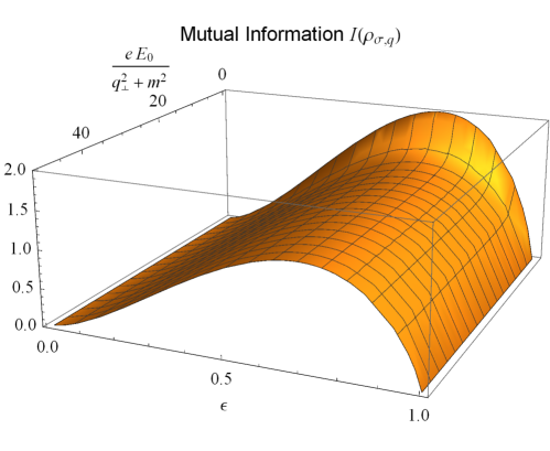
Figure 1: The mutual information $I(\rho_{\sigma,\mathbf{q}})$ as a function of the dimensionless parameters $\frac{eE_{0}}{q_{\perp}^{2}+m^{2}}$ and $\varepsilon$, where $E_{0}$ is the strength of the constant electric field, and $\varepsilon$ is the coefficient parameter of the initial entangled state.

The dependence of the mutual information $I(\rho_{\sigma,\mathbf{q}})$ on the electric field $E_{0}$ and the parameter $\varepsilon$ is shown in Fig. 1. For a fixed value of $\varepsilon$, $I(\rho_{\sigma,\mathbf{q}})$ monotonically decreases with the increase of the electric field $E_{0}$ and asymptotically approaches a certain nonvanishing value independent of $E_{0}$. For $\varepsilon$ less or larger than $\frac{1}{\sqrt{2}}$, the closer to $\frac{1}{\sqrt{2}}$ the parameter $\varepsilon$ is, the quicker $I(\rho_{\sigma,\mathbf{q}})$ decreases with the increase of $E_{0}$ when $E_{0}$ is small. For any given value of $E_{0}$ and for $\varepsilon$ less or larger than $\frac{1}{\sqrt{2}}$, the farther to $\frac{1}{\sqrt{2}}$ the parameter $\varepsilon$ is, the smaller $I(\rho_{\sigma,\mathbf{q}})$ is. The mutual information $I(\rho_{\sigma,\mathbf{q}})$ becomes zero as $\varepsilon=0$ or $1$, in which case the mutual information vanishes even in the absence of the electric field.

We use logarithmic negativity to measure the entanglement. After making the partial transpose of the density matrix $\rho_{\sigma,\mathbf{q}}$ with respect to $\sigma$, we obtain

$$\rho^{\mathrm{T}_{\sigma}}_{\sigma,\mathbf{q}}= \frac{\varepsilon^{2}}{|\alpha_{\mathbf{q}}|^{2}}\sum_{n=0}^{\infty}\left|\frac{\beta_{\mathbf{q}}}{\alpha_{\mathbf{q}}}\right|^{2n}|\uparrow,n_{\mathbf{q}}\rangle\langle\uparrow,n_{\mathbf{q}}|$$

$$+\frac{\varepsilon\sqrt{1-\varepsilon^{2}}}{|\alpha_{\mathbf{q}}|^{2}\alpha_{\mathbf{q}}}\sum_{n=0}^{\infty}\left|\frac{\beta_{\mathbf{q}}}{\alpha_{\mathbf{q}}}\right|^{2n}\sqrt{n+1}|\downarrow,n_{\mathbf{q}}\rangle\langle\uparrow,(n+1)_{\mathbf{q}}|$$

$$+\frac{\varepsilon\sqrt{1-\varepsilon^{2}}}{|\alpha_{\mathbf{q}}|^{2}\alpha^{*}_{\mathbf{q}}}\sum_{n=0}^{\infty}\left|\frac{\beta_{\mathbf{q}}}{\alpha_{\mathbf{q}}}\right|^{2n}\sqrt{n+1}|\uparrow,(n+1)_{\mathbf{q}}\rangle\langle\downarrow,n_{\mathbf{q}}|$$

$$+\frac{1-\varepsilon^{2}}{|\alpha_{\mathbf{q}}|^{4}}\sum_{n=0}^{\infty}\left|\frac{\beta_{\mathbf{q}}}{\alpha_{\mathbf{q}}}\right|^{2n}(n+1)|\downarrow,(n+1)_{\mathbf{q}}\rangle\langle\downarrow,(n+1)_{\mathbf{q}}|,$$ (22)

which is a block matrix in the subspace of $\{|\uparrow,(n+1)_{\mathbf{q}}\rangle,|\downarrow,n_{\mathbf{q}}\rangle\}$, $(n=0,1,2,\cdots)$. Therefore the eigenvalues of $\rho^{\mathrm{T}_{\sigma}}_{\sigma,\mathbf{q}}$ are

$$\frac{\varepsilon^{2}}{|\alpha_{\mathbf{q}}|^{2}},$$

$$\ \ \ \ \ \ \ \frac{1}{2|\alpha_{\mathbf{q}}|^{2}}\left|\frac{\beta_{\mathbf{q}}}{\alpha_{\mathbf{q}}}\right|^{2n}\left[\ \left|\frac{\beta_{\mathbf{q}}}{\alpha_{\mathbf{q}}}\right|^{2}\varepsilon^{2}+\frac{n(1-\varepsilon^{2})}{|\beta_{\mathbf{q}}|^{2}}\right.\pm$$

$$\left.\sqrt{\left(\left|\frac{\beta_{\mathbf{q}}}{\alpha_{\mathbf{q}}}\right|^{2}\varepsilon^{2}+\frac{n(1-\varepsilon^{2})}{|\beta_{\mathbf{q}}|^{2}}\right)^{2}+\frac{4\varepsilon^{2}(1-\varepsilon^{2})}{|\alpha_{\mathbf{q}}|^{2}}}\ \right],\ \ n=0,1,2,\cdots\cdots$$ (23)

Thus the logarithmic negativity is

$$N(\rho_{\sigma,\mathbf{q}})$$

$$=\log_{2}\left[\frac{\varepsilon^{2}}{|\alpha_{\mathbf{q}}|^{2}}+\sum_{n=0}^{\infty}\frac{|\beta_{\mathbf{q}}|^{2n}}{|\alpha_{\mathbf{q}}|^{2(n+1)}}\sqrt{\left(\left|\frac{\beta_{\mathbf{q}}}{\alpha_{\mathbf{q}}}\right|^{2}\varepsilon^{2}+\frac{n(1-\varepsilon^{2})}{|\beta_{\mathbf{q}}|^{2}}\right)^{2}+\frac{4\varepsilon^{2}(1-\varepsilon^{2})}{|\alpha_{\mathbf{q}}|^{2}}}\ \right],$$ (24)

which describes the quantum entanglement between $\sigma$ and $\mathbf{q}$. $N(\rho_{\sigma,\mathbf{q}})=\log_{2}[1+2\varepsilon\sqrt{1-\varepsilon^{2}}]$ when $E_{0}=0$.

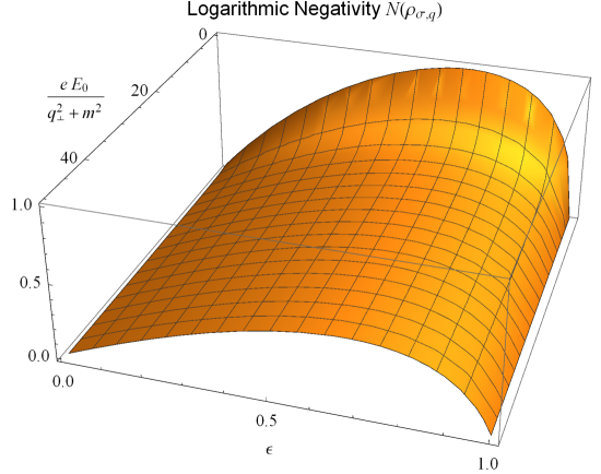
Figure 2: The logarithmic negativity $N(\rho_{\sigma,\mathbf{q}})$ as a function of the dimensionless parameters $\frac{eE_{0}}{q_{\perp}^{2}+m^{2}}$ and $\varepsilon$, where $E_{0}$ is the strength of the constant electric field, and $\varepsilon$ is the coefficient parameter of the initial entangled state.

Fig. 2 shows how the logarithmic negativity $N(\rho_{\sigma,\mathbf{q}})$ depends on the strength of the electric field $E_{0}$ and the parameter $\varepsilon$. The variation trend of $N(\rho_{\sigma,\mathbf{q}})$ with respect to $E_{0}$ and $\varepsilon$ is similar to that of $I(\rho_{\sigma,\mathbf{q}})$. But when $E_{0}$ is small, $N(\rho_{\sigma,\mathbf{q}})$ decreases more rapidly with the increase of $E_{0}$ than $I(\rho_{\sigma,\mathbf{q}})$ does, indicating that the entanglement is more sensitive to the coupling with the electric field. Like $I(\rho_{\sigma,\mathbf{q}})$, $N(\rho_{\sigma,\mathbf{q}})$ monotonically decreases with the increase of the electric field $E_{0}$ and approaches a certain nonzero asymptotic value as $E_{0}\rightarrow\infty$.

The Schwinger effect of two entangled fermions of momenta $\mathbf{p}$ and $\mathbf{q}$ lidaishi can reduce effectively to a fermion counterpart of our present bosonic problem, under the constraint that the electric field does not couple the mode $\mathbf{p}$, thus fixing the Bogoliubov coefficients of the $\mathbf{p}$ mode to be $\alpha_{\mathbf{p}}=0$, $\beta_{\mathbf{p}}=1$, thereby reducing mode $\mathbf{p}$ to our qubit $\sigma$. With the increase of $E_{0}$, the monotonic decrease towards $0$ of the mutual information and entanglement between fermionic mode $\mathbf{p}$ and mode $\mathbf{q}$ reduces to those between the qubit $\mathbf{\sigma}$ and fermionic mode $\mathbf{q}$ here. The boson-fermion comparison will be discussed in the summary.

It is also interesting to make comparison with the bosons in Unruh effect fuentes1 ; Eduardo ; Pan and near a dilaton black hole Jieci , with the role of the electric field in our case replaced as the acceleration, but the Bogoliubov coefficient that is the counterpart of $|\beta_{\mathbf{k}}|^{2}$ can be arbitrarily large, making the entanglement disappear in the limiting cases. In contrast, in our present case, $|\beta_{\mathbf{k}}|^{2}<1$, consequently the entanglement in $\rho_{\sigma,\mathbf{q}}$ persists as $E_{0}\rightarrow\infty$.

5 Correlation and entanglement between the qubit $\sigma$ and the mode $\mathbf{-q}$

Now we study the correlation and the entanglement between $\sigma$ and $\mathbf{-q}$. Tracing out the mode $\mathbf{q}$, we obtain the reduced density matrix of $\sigma$ and $\mathbf{-q}$, $\rho_{\sigma,\mathbf{-q}}={\mathrm{Tr}}_{\mathbf{q}}(\rho_{\sigma,\mathbf{q},\mathbf{-q}})$, as

$$\rho_{\sigma,\mathbf{-q}}= \frac{\varepsilon^{2}}{|\alpha_{\mathbf{q}}|^{2}}\sum_{n=0}^{\infty}\left|\frac{\beta_{\mathbf{q}}}{\alpha_{\mathbf{q}}}\right|^{2n}|\uparrow,n_{\mathbf{-q}}\rangle\langle\uparrow,n_{\mathbf{-q}}|$$

$$+\frac{\varepsilon\sqrt{1-\varepsilon^{2}}\beta^{*}_{\mathbf{q}}}{|\alpha_{\mathbf{q}}|^{4}}\sum_{n=0}^{\infty}\left|\frac{\beta_{\mathbf{q}}}{\alpha_{\mathbf{q}}}\right|^{2n}\sqrt{n+1}|\uparrow,(n+1)_{\mathbf{-q}}\rangle\langle\downarrow,n_{\mathbf{-q}}|$$

$$+\frac{\varepsilon\sqrt{1-\varepsilon^{2}}\beta_{\mathbf{q}}}{|\alpha_{\mathbf{q}}|^{4}}\sum_{n=0}^{\infty}\left|\frac{\beta_{\mathbf{q}}}{\alpha_{\mathbf{q}}}\right|^{2n}\sqrt{n+1}|\downarrow,n_{\mathbf{-q}}\rangle\langle\uparrow,(n+1)_{\mathbf{-q}}|$$

$$+\frac{1-\varepsilon^{2}}{|\alpha_{\mathbf{q}}|^{4}}\sum_{n=0}^{\infty}\left|\frac{\beta_{\mathbf{q}}}{\alpha_{\mathbf{q}}}\right|^{2n}(n+1)|\downarrow,n_{\mathbf{-q}}\rangle\langle\downarrow,n_{\mathbf{-q}}|,$$ (25)

which is a block matrix in the subspace of $\{|\uparrow,n_{\mathbf{q}}\rangle,|\downarrow,(n-1)_{\mathbf{q}}\rangle\}$, $(n=1,2,3,\cdots)$, thus the non-zero eigenvalues of $\rho_{\sigma,\mathbf{-q}}$ are

$$\frac{1}{|\alpha_{\mathbf{q}}|^{2}}\left|\frac{\beta_{\mathbf{q}}}{\alpha_{\mathbf{q}}}\right|^{2n}\left[\varepsilon^{2}+\frac{n(1-\varepsilon^{2})}{|\beta_{\mathbf{q}}|^{2}}\right],\ \ n=0,1,2,\cdots.$$ (26)

Tracing out the field mode $\mathbf{-q}$ in $\rho_{\sigma,\mathbf{-q}}$ yields $\rho_{\sigma}={\mathrm{Tr}}_{\mathbf{-q}}(\rho_{\sigma,\mathbf{-q}})$, which is

$$\rho_{\sigma}=\varepsilon^{2}|0_{p}\rangle\langle 0_{\sigma}|+(1-\varepsilon^{2})|1_{p}\rangle\langle 1_{\sigma}|,$$ (27)

with eigenvalues $\varepsilon^{2}$, $1-\varepsilon^{2}$.

Tracing out $\sigma$ in $\rho_{\sigma,\mathbf{-q}}$ yields $\rho_{\mathbf{-q}}={\mathrm{Tr}}_{\sigma}(\rho_{\sigma,\mathbf{-q}})$, which is

$$\rho_{\mathbf{-q}}=\frac{1}{|\alpha_{\mathbf{q}}|^{2}}\sum_{n=0}^{\infty}\left|\frac{\beta_{\mathbf{q}}}{\alpha_{\mathbf{q}}}\right|^{2n}\left[\varepsilon^{2}+\frac{(n+1)(1-\varepsilon^{2})}{|\alpha_{\mathbf{q}}|^{2}}\right]|n_{\mathbf{-q}}\rangle\langle n_{\mathbf{-q}}|,$$ (28)

with eigenvalues

$$\frac{1}{|\alpha_{\mathbf{q}}|^{2}}\left|\frac{\beta_{\mathbf{q}}}{\alpha_{\mathbf{q}}}\right|^{2n}\left[\varepsilon^{2}+\frac{(n+1)(1-\varepsilon^{2})}{|\alpha_{\mathbf{q}}|^{2}}\right],\ \ n=0,1,2,\cdots.$$ (29)

According to the definition of the mutual information between modes $\sigma$ and $\mathbf{-q}$, we have

$$I(\rho_{\sigma,\mathbf{-q}})$$

$$=-\varepsilon^{2}\log_{2}\varepsilon^{2}-(1-\varepsilon^{2})\log_{2}(1-\varepsilon^{2})$$

$$+\sum_{n=0}^{\infty}\frac{|\beta_{\mathbf{q}}|^{2n}}{|\alpha_{\mathbf{q}}|^{2(n+1)}}\left[\varepsilon^{2}+\frac{n(1-\varepsilon^{2})}{|\beta_{\mathbf{q}}|^{2}}\right]\log_{2}\left[\frac{|\beta_{\mathbf{q}}|^{2n}}{|\alpha_{\mathbf{q}}|^{2(n+1)}}\left(\varepsilon^{2}+\frac{n(1-\varepsilon^{2})}{|\beta_{\mathbf{q}}|^{2}}\right)\right]$$

$$-\sum_{n=0}^{\infty}\frac{|\beta_{\mathbf{q}}|^{2n}}{|\alpha_{\mathbf{q}}|^{2(n+1)}}\left[\varepsilon^{2}+\frac{(n+1)(1-\varepsilon^{2})}{|\alpha_{\mathbf{q}}|^{2}}\right]\log_{2}\left[\frac{|\beta_{\mathbf{q}}|^{2n}}{|\alpha_{\mathbf{q}}|^{2(n+1)}}\left(\varepsilon^{2}+\frac{(n+1)(1-\varepsilon^{2})}{|\alpha_{\mathbf{q}}|^{2}}\right)\right].$$ (30)

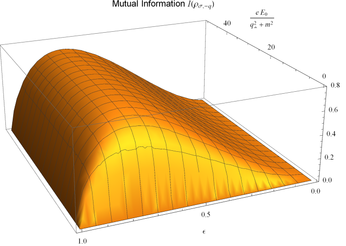
Figure 3: The mutual information $I(\rho_{\sigma,\mathbf{-q}})$ as a function of the dimensionless parameters $\frac{eE_{0}}{q_{\perp}^{2}+m^{2}}$ and $\varepsilon$, where $E_{0}$ is the strength of the constant electric field, and $\varepsilon$ is the coefficient parameter of the initial entangled state.

The dependence of the mutual information $I(\rho_{\sigma,\mathbf{-q}})$ on the electric field $E_{0}$ and the parameter $\varepsilon$ is shown in Fig. 3. $I(\rho_{\sigma,\mathbf{-q}})$ monotonically increases with the increase of the electric field $E_{0}$, and asymptotically approaches a certain value independent of $E_{0}$. For $\varepsilon$ larger or smaller than $\frac{1}{\sqrt{2}}$, the closer to $\frac{1}{\sqrt{2}}$ the parameter $\varepsilon$ is, the larger the asymptotic value is. Moreover, when $E_{0}$ is small, for $\varepsilon$ larger or smaller than $\frac{1}{\sqrt{2}}$, the closer to $\frac{1}{\sqrt{2}}$ the parameter $\varepsilon$ is, the quicker $I(\rho_{\sigma,\mathbf{-q}})$ increases with the increase of $E_{0}$, and the larger the value of $I(\rho_{\sigma,\mathbf{-q}})$ is.

Now we calculate the logarithmic negativity of $\rho_{\sigma,\mathbf{-q}}$. After making the partial transpose of the density matrix $\rho_{\sigma,\mathbf{-q}}$ with respect to the mode $p$, one obtains

$$\rho^{\mathrm{T}_{\sigma}}_{\sigma,\mathbf{-q}}= \frac{\varepsilon^{2}}{|\alpha_{\mathbf{q}}|^{2}}\sum_{n=0}^{\infty}\left|\frac{\beta_{\mathbf{q}}}{\alpha_{\mathbf{q}}}\right|^{2n}|\uparrow,n_{\mathbf{-q}}\rangle\langle\uparrow,n_{\mathbf{-q}}|$$

$$+\frac{\varepsilon\sqrt{1-\varepsilon^{2}}\beta^{*}_{\mathbf{q}}}{|\alpha_{\mathbf{q}}|^{4}}\sum_{n=0}^{\infty}\left|\frac{\beta_{\mathbf{q}}}{\alpha_{\mathbf{q}}}\right|^{2n}\sqrt{n+1}|\downarrow,(n+1)_{\mathbf{-q}}\rangle\langle\uparrow,n_{\mathbf{-q}}|$$

$$+\frac{\varepsilon\sqrt{1-\varepsilon^{2}}\beta_{\mathbf{q}}}{|\alpha_{\mathbf{q}}|^{4}}\sum_{n=0}^{\infty}\left|\frac{\beta_{\mathbf{q}}}{\alpha_{\mathbf{q}}}\right|^{2n}\sqrt{n+1}|\uparrow,n_{\mathbf{-q}}\rangle\langle\downarrow,(n+1)_{\mathbf{-q}}|$$

$$+\frac{1-\varepsilon^{2}}{|\alpha_{\mathbf{q}}|^{4}}\sum_{n=0}^{\infty}\left|\frac{\beta_{\mathbf{q}}}{\alpha_{\mathbf{q}}}\right|^{2n}(n+1)|\downarrow,n_{\mathbf{-q}}\rangle\langle\downarrow,n_{\mathbf{-q}}|,$$ (31)

which is a block matrix in the subspace of $\{|\uparrow,n_{\mathbf{q}}\rangle,|\downarrow,(n+1)_{\mathbf{q}}\rangle\}$, with eigenvalues

$$\frac{1-\varepsilon^{2}}{|\alpha_{\mathbf{q}}|^{4}},$$

$$\ \ \ \ \ \ \ \frac{1}{2|\alpha_{\mathbf{q}}|^{2}}\left|\frac{\beta_{\mathbf{q}}}{\alpha_{\mathbf{q}}}\right|^{2n}\left[\ \varepsilon^{2}+\frac{(n+2)(1-\varepsilon^{2})|\beta_{\mathbf{q}}|^{2}}{|\alpha_{\mathbf{q}}|^{4}}\right.\pm$$

$$\left.\sqrt{\left(\varepsilon^{2}+\frac{(n+2)(1-\varepsilon^{2})|\beta_{\mathbf{q}}|^{2}}{|\alpha_{\mathbf{q}}|^{4}}\right)^{2}-\frac{4\varepsilon^{2}(1-\varepsilon^{2})|\beta_{\mathbf{q}}|^{2}}{|\alpha_{\mathbf{q}}|^{4}}}\ \right],\ \ n=0,1,2,\cdots.$$ (32)

Thus the logarithmic negativity of $\rho_{\sigma,\mathbf{-q}}$ is

$$N(\rho_{\sigma,\mathbf{-q}}) =\log_{2}\left[\frac{1-\varepsilon^{2}}{|\alpha_{\mathbf{q}}|^{4}}+\sum_{n=0}^{\infty}\frac{|\beta_{\mathbf{q}}|^{2n}}{|\alpha_{\mathbf{q}}|^{2(n+1)}}\left(\varepsilon^{2}+\frac{(n+2)(1-\varepsilon^{2})|\beta_{\mathbf{q}}|^{2}}{|\alpha_{\mathbf{q}}|^{4}}\right)\right]$$

$$=\log_{2}1=0,$$ (33)

which means starting from the initial state (13 ) with any value of the parameter $\varepsilon$, which is entangled between $\sigma$ and in mode $\mathbf{q}$, with the action of the electric field, the entanglement between $\sigma$ and out mode $\mathbf{-q}$ always vanishes.

From the expressions of the mutual information of $\rho_{\sigma,\mathbf{q}}$ and $\rho_{\sigma,\mathbf{-q}}$, we obtain

$$I(\rho_{\sigma,\mathbf{q}})+I(\rho_{\sigma,\mathbf{-q}})=-2[\varepsilon^{2}\log_{2}\varepsilon^{2}+(1-\varepsilon^{2})\log_{2}(1-\varepsilon^{2})],$$ (34)

implying that Schwinger effect redistributes the total correlation in the initial entangled state, into $\rho_{\sigma,\mathbf{q}}$ and $\rho_{\sigma,\mathbf{-q}}$. However, there is no such an identity for the logarithmic negativity, hence Schwinger effect does not redistribute quantum entanglement. The reason is that the qubit is not coupled with the electric field. In the fermion model studied previously lidaishi , even when reduced to the problem of an uncoupled qubit and the fermionic mode coupled with the electric field, redistribution exists both in mutual information and in logarithmic negativity. See Eqs. (38-39) in Ref.  lidaishi , where the fermionic mode coupled with the electric field is denoted as $\mathbf{p}$, and the uncoupled mode $\mathbf{q}$ is equivalent to a qubit.

6 Effect of a pulsed electric field

Now we investigate the effect of a pulsed electric field. Consider a Sauter-type electric field $E(t)=E_{0}\mathrm{sech}^{2}(t/\tau)$ along $z$ direction, where $\tau$ is the width of the pulsed electric field sauter . The gauge potential $A_{\mu}$ can be chosen as

$$A_{\mu}=\left(0,0,0,-E_{0}\tau\tanh\left(\frac{t}{\tau}\right)\right),$$ (35)

for which the Bogoliubov transformation yields kim ; Ebadi

$$|\alpha_{\mathbf{k}}|^{2}=\frac{\cosh[\pi\tau(\omega^{\mathrm{out}}_{k}+\omega^{\mathrm{in}}_{k})]+\cosh(2\pi\lambda)}{2\sinh(\pi\tau\omega^{\mathrm{in}}_{k})\sinh\ (\pi\tau\omega^{\mathrm{out}}_{k})},$$ (36)

$$|\beta_{\mathbf{k}}|^{2}=\frac{\cosh[\pi\tau(\omega^{\mathrm{out}}_{k}-\omega^{\mathrm{in}}_{k})]+\cosh(2\pi\lambda)}{2\sinh(\pi\tau\omega^{\mathrm{in}}_{k})\sinh\ (\pi\tau\omega^{\mathrm{out}}_{k})},$$ (37)

where

$$\lambda=\sqrt{(eE_{0}\tau^{2})^{2}-\frac{1}{4}},$$ (38)

$$\omega^{\mathrm{in}}_{k}=\sqrt{(k_{z}+eE_{0}\tau)^{2}+k^{2}_{\bot}+m^{2}},$$ (39)

$$\omega^{\mathrm{out}}_{k}=\sqrt{(k_{z}-eE_{0}\tau)^{2}+k^{2}_{\bot}+m^{2}}.$$ (40)

As $\tau\to 0$, $E(t)\to 0$, then $|\alpha_{\mathbf{k}}|^{2}\to 1$ and $|\beta_{\mathbf{k}}|^{2}\to 0$, reducing the problem to the case without the electric field. As $\tau\to+\infty$, $E(t)\to E_{0}$, which means $|\alpha_{\mathbf{k}}|^{2}$ and $|\beta_{\mathbf{k}}|^{2}$ reduce to the values in the case of the constant electric field.

The analyses and calculations for $\rho_{\sigma,\mathbf{q}}$ and $\rho_{\sigma,\mathbf{-q}}$ above for the case of a constant electric field can be applied to the pulsed electric field, but with $|\alpha_{\mathbf{k}}|^{2}$ and $|\beta_{\mathbf{k}}|^{2}$ now given in Eqs. (36) and (37). Hence the mutual information and logarithmic negativity now depend on not only $E_{0}$ but also $\tau$.

In parallel with the above study on a constant electric field, we first investigate the influence of a pulsed electric field on the entanglement and correlation between $\sigma$ and mode $\mathbf{q}$.

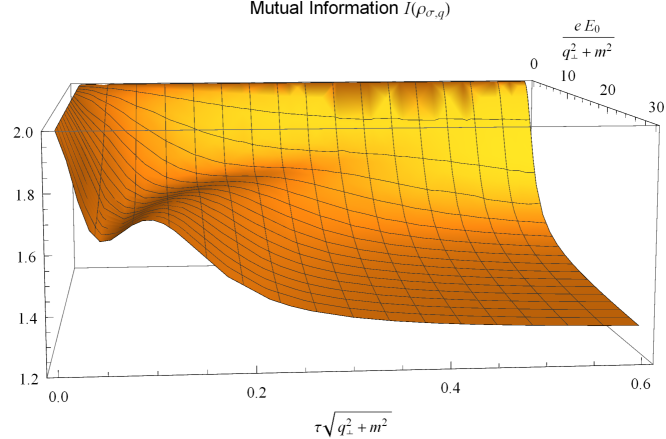
Figure 4: The mutual information $I(\rho_{\sigma,\mathbf{q}})$ as a function of the dimensionless parameters $\frac{eE_{0}}{q_{\perp}^{2}+m^{2}}$ and $\tau\sqrt{q_{\perp}^{2}+m^{2}}$. It is assumed that $q_{z}=\sqrt{q_{\perp}^{2}+m^{2}}$, $\varepsilon=1/\sqrt{2}$.

The influence of the pulsed electric field on the mutual information $I(\rho_{\sigma,\mathbf{q}})$ is shown in Fig. 4, which indicates its dependence on the strength $E_{0}$ and the width $\tau$ of the pulsed electric field. For $E_{0}$ smaller than a certain value, with the increase of $\tau$, $I(\rho_{\sigma,\mathbf{q}})$ monotonically decreases and approaches the asymptotic value dependent on $E_{0}$ as $\tau\rightarrow\infty$. For $E_{0}$ larger than a certain value, with the increase of $\tau$, $I(\rho_{\sigma,\mathbf{q}})$ first decreases to a minimum and then increases to a maximum before finally decreases and approaches asymptotically a value dependent on $E_{0}$ as $\tau\rightarrow\infty$. The larger $E_{0}$ is, the smaller the values of $\tau$ corresponding to the minimum and the maximum of $I(\rho_{\sigma,\mathbf{q}})$. When $\tau$ is small, with the increase of $E_{0}$, $I(\rho_{\sigma,\mathbf{q}})$ decreases to a minimum and then increases to a maximum, and finally decreases and approaches asymptotically a certain value independent of $E_{0}$. For a given value of $\tau$, the variation trend of $I(\rho_{\sigma,\mathbf{q}})$ with respect to $E_{0}$ is opposite to that of $I(\rho_{\sigma,\mathbf{q}})$ with respect to $\tau$ for a given value of $E_{0}$. Moreover, When $\tau$ is smaller than a certain value, the larger the values of $E_{0}$ corresponding to the minimum and the maximum of $I(\rho_{\sigma,\mathbf{q}})$. When $\tau$ is larger than a certain value, $I(\rho_{\sigma,\mathbf{q}})$ decreases monotonically with the increase of $E_{0}$ and asymptotically approaches a value independent of $E_{0}$. As $\tau\rightarrow\infty$, the dependence of $I(\rho_{\sigma,\mathbf{q}})$ on $E_{0}$ is the same as that the case of constant electric field for $\varepsilon=1/\sqrt{2}$, as shown in Fig. 1.

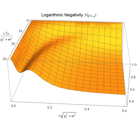
Figure 5: The logarithmic negativity $N(\rho_{\sigma,\mathbf{q}})$ as a function of the dimensionless parameters $\frac{eE_{0}}{q_{\perp}^{2}+m^{2}}$ and $\tau\sqrt{q_{\perp}^{2}+m^{2}}$. It is assumed that $q_{z}=\sqrt{q_{\perp}^{2}+m^{2}}$, $\varepsilon=1/\sqrt{2}$.

As shown in Fig. 5, the dependence of $N(\rho_{\sigma,\mathbf{q}})$ on $E_{0}$ and $\tau$ is entirely similar to that of $I(\rho_{\sigma,\mathbf{q}})$, but the values of $\tau$ and $E_{0}$ corresponding to the minima and maxima of $N(\rho_{\sigma,\mathbf{q}})$ are different from those of $I(\rho_{\sigma,\mathbf{q}})$. As $\tau\rightarrow\infty$ , the case of the constant electric field is also recovered, as shown in Fig. 2 for $\varepsilon=1/\sqrt{2}$.

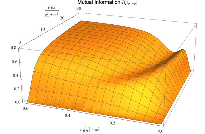
Figure 6: The mutual information $I(\rho_{\sigma,\mathbf{-q}})$ as a function of the dimensionless parameters $\frac{eE_{0}}{q_{\perp}^{2}+m^{2}}$ and $\tau\sqrt{q_{\perp}^{2}+m^{2}}$. It is assumed that $q_{z}=\sqrt{q_{\perp}^{2}+m^{2}}$, $\varepsilon=1/\sqrt{2}$.

The correlation between $\sigma$ and $\mathbf{-q}$ is exactly a complement of that between $\sigma$ and $\mathbf{q}$, as indicated in Eq. (34). Therefore the dependence of $I(\rho_{\sigma,\mathbf{-q}})$ on the pulsed electric field is exactly opposite to that of $I(\rho_{\sigma,\mathbf{-q}})$, as shown in Fig. 6.

7 Summary and discussions

In this paper, we consider a state in which a qubit is entangled with a bosonic mode. The scalar field is coupled with an electric field.

We have studied how the total correlation and the quantum entanglement in $\rho_{\sigma,\mathbf{q}}$ and $\rho_{\sigma,\mathbf{-q}}$ depend on the electric field. In the case of a constant electric field, the mutual information $I(\rho_{\sigma,\mathbf{q}})$ decreases with the increase of the strength of the electric field and approaches a certain nonvanishing value, implying that the total correlation between qubit $\sigma$ and mode $\mathbf{q}$ never vanishes. Similarly, the logarithmic negativity $N(\rho_{\sigma,\mathbf{q}})$ decreases with the increase of the strength of the electric field and approaches a certain nonvanishing value, implying that the entanglement in $\rho_{\sigma,\mathbf{q}}$ never vanishes even if the strength of the electric field tends to infinity. For $\rho_{\sigma,\mathbf{-q}}$, the mutual information $I(\rho_{\sigma,\mathbf{-q}})$ increases with the increase of the strength of the electric field and asymptotically approaches a certain value. In fact, the sum of $I(\rho_{\sigma,\mathbf{q}})$ and $I(\rho_{\sigma,\mathbf{-q}})$ is a constant determined by the initial state.

However no matter how strong the electric field is, the logarithmic negativity $N(\rho_{\sigma,\mathbf{-q}})$ remains zero, i.e. $\sigma$ and mode $\mathbf{-q}$ remain unentangled, though Schwinger effect does decrease the entanglement between $\sigma$ and mode $\mathbf{q}$. We have also considered Schwinger effect of a pulsed electric field, for which the pulse width plays a role.

The bosonic correlation and entanglement an electric field are quite different from those of the fermionic entanglement  lidaishi . In the bosonic case, with the increase of the electric field strength, the correlation (measured as mutual information) and the entanglement (measured as mutual information) between the qubit and the original particle mode decrease towards non-zero asymptotic values, while the entanglement between the qubit and the antiparticle mode remains zero though the correlation increases towards an asymptotic value. In the fermionic case, with the increase of the electric field strength, the correlation and the entanglement between the qubit and the original particle mode decrease towards zero, while both the correlation and the entanglement between the qubit and the antiparticle mode increases towards values of those between the qubit and the particle mode.

This work is supported by National Natural Science Foundation of China (Grant No. 11574054).

References

(1) J. Schwinger, Phys. Rev. 82, 664 (1951).
(2) A. Di Piazza, C. Müller, K. Z. Hatsagortsyan, and C. H. Keitel, Rev. Mod. Phys. 84, 1177 (2012).
(3) Y. Shi, Phys. Rev. D 70, 105001 (2004).
(4) Z. Ebadi and B. Mirza, Ann. Phys. (NY), 351, 363 (2014).
(5) S. P. Gavrilov, D. M. Gitman, and A. A. Shishmarev, Phys. Rev. A 91, 052106 (2015).
(6) Y. Li, Y. Dai and Y. Shi, Phys. Rev. D 95, 036006 (2017).
(7) M. A. Nielsen and I. Chuang, Quantum Computation and Quantum Information (Cambridge University, Cambridge, 2000).
(8) G. Vidal and R. F. Werner, Phys. Rev. A 65, 032314 (2002).
(9) R. Brout, Phys. Rep. 260, 329 (1995).
(10) S. P. Kim, H. K. Lee, and Y. Yoon, Phys. Rev. D 78, 105013 (2008), and references therein.
(11) I. Fuentes-Schuller and R. B. Mann, Phys. Rev. Lett. 95, 120404 (2005).
(12) E. Martín-Martínez and J. León, Phys. Rev. A 81, 052305 ( 2010).
(13) Q. Pan and J. Jing, Phys. Rev. A 77, 024302 (2008).
(14) J. Wang, Q. Pan, S. Chen, and J. Jing, Phys. Lett B 677, 186 (2009).