Equilibrium properties of the lattice system with SALR interaction potential on a square lattice: quasi-chemical approximation versus Monte Carlo simulation

Abstract

The lattice system with competing interactions that models biological objects (colloids, ensembles of protein molecules, etc.) is considered. This system is the lattice fluid on a square lattice with attractive interaction between nearest neighbours and repulsive interaction between next-next-nearest neighbours. The geometric order parameter is introduced for describing the ordered phases in this system. The critical value of the order parameter is estimated and the phase diagram of the system is constructed. The simple quasi-chemical approximation (QChA) is proposed for the system under consideration. The data of Monte Carlo simulation of equilibrium properties of the model are compared with the results of QChA. It is shown that QChA provides reasonable semiquantitative results for the systems studied and can be used as the basis for next order approximations.

Key words: lattice fluid model, competing interaction, order-disorder phase transition, Monte Carlo simulation, quasi-chemical approximation, phase diagram

PACS: 05.10.Ln, 64.60.De, 64.60.Cn

Abstract

Ðîçãëÿäàєòüñÿ ґðàòêîâà ñèñòåìà ç êîíêóðåíòíèìè âçàєìîäiÿìè, ùî ìîäåëþє áiîëîãiчíi îá’єêòè (êîëî¿äè, àíñàìáëi ïðîòå¿íîâèõ ìîëåêóë i ò.ä.). Öÿ ñèñòåìà ïðåäñòàâëÿєòüñÿ ґðàòêîâèì ïëèíîì íà êâàäðàòíié ґðàòöi ç ïðèòÿãàëüíîþ âçàєìîäiєþ ìiæ íàéáëèæчèìè ñóñiäàìè i âiäøòîâõóâàëüíîþ âçàєìîäiєþ ìiæ íàñòóïíèìè çà íàñòóïíèìè äî íàéáëèæчèõ ñóñiäiâ. Äëÿ îïèñó âïîðÿäêîâàíî¿ ôàçè â òàêié ñèñòåìi ââîäèòüñÿ ãåîìåòðèчíèé ïàðàìåòð ïîðÿäêó. Çðîáëåíà îöiíêà êðèòèчíîãî çíàчåííÿ ïàðàìåòðà ïîðÿäêó i ïîáóäîâàíà ôàçîâà äiàãðàìà ñèñòåìè. Äëÿ ñèñòåìè, ùî ðîçãëÿäàєòüñÿ, çàïðîïîíîâàíî ïðîñòå êâàçiõiìiчíå íàáëèæåííÿ (ÊÕÍ). Äàíi ñèìóëÿöié Ìîíòå Êàðëî ðiâíîâàæíèõ âëàñòèâîñòåé ìîäåëi ïîðiâíþþòüñÿ ç ðåçóëüòàòàìè ÊÕÍ. Ïîêàçàíî, ùî ÊÕÍ çàáåçïåчóє ïðèéíÿòíi íàïiâêiëüêiñíi ðåçóëüòàòè äëÿ ñèñòåìè, ùî âèâчàєòüñÿ, i ìîæå âèêîðèñòîâóâàòèñÿ ÿê áàçèñ äëÿ íàñòóïíèõ íàáëèæåíü.

Ключовi слова: ґðàòêîâà ìîäåëü ïëèíó, êîíêóðóþчà âçàєìîäiÿ, ôàçîâèé ïåðåõiä ïîðÿäîê-áåçëàä, ñèìóëÿöi¿ Ìîíòå Êàðëî, êâàçiõiìiчíå íàáëèæåííÿ, ôàçîâà äiàãðàìà

1 Introduction

At present, there is a great interest in studying the processes of self-organization and self-assembly in systems of a nanoscale range. As the elements of such systems are supramolecular formations with a sufficiently large molecular mass, this leads to low velocities of their thermal motion and to large, on the molecular scale, characteristic times of the processes within the system. At the same time, the interaction between these elements is very complex. Despite their rather large dimensions, the interactions remain of the same order as the thermal energy. This leads to a large variety of possibilities for various phase transitions in such systems at room temperature. Examples are solutions of protein molecules [1], clays and soil suspensions [2], ecosystems [3], etc.

In general, structure elements of such systems attract each other at small distances due, for example, to the Van der Waals attraction, and repulse on longer separations because of the electrostatic interactions (SALR systems, short-range attractive and long-range repulsive interaction) [4, 5]. In the case of biological molecules, repulsion can also be caused by elastic deformations of the lipid membranes. In any case, the attraction between the structural elements of the system ensures the phase separation, and repulsion — the formation of clusters.

One of the simplest methods for investigating the general properties of SALR systems is to consider their lattice models. These models are simple enough and allow one to make a detailed analysis both by analytical methods and computer simulation, using the Monte Carlo method. A large number of common properties of such systems can be obtained within these frameworks.

For example, in papers [6, 7], a lattice fluid was studied with attraction of nearest neighbours and repulsion of the third neighbours on a plane triangular lattice. Possible configurations of the ensemble of particles were investigated. A phase diagram of the system in the mean field approximation and by Monte Carlo simulation was constructed. It revealed the existence of several phase transitions in the system.

In [8] the generalized quasi-chemical approximation (QChA) was proposed for lattice systems with SALR interaction potential on a triangular lattice. This approximation has demonstrated its applicability for estimating the equilibrium properties of the model in the disordered phase.

In this paper, we present the results for a similar model of the lattice fluid on a square lattice and propose a geometric order parameter, which makes it possible to investigate the ordered phases in the system.

2 The model and its order parameter

We consider the lattice fluid consisting of $n$ particles on a square lattice of $N$ lattice sites. Multiple occupation of sites is forbidden. Particles that occupy nearest lattice sites and sites that are neighbours of the third order interact with each other. The interaction energies are equal to $J_{1}$ and $J_{3}$, respectively. It is assumed that $J_{1}=-J<0$, and $J_{3}=3J>0$, which corresponds to the attraction of the nearest neighbours and the repulsion of the third ones. The second, forth and more distant neighbours are considered as noninteracting ones.

The simulation of the equilibrium characteristics of the system under consideration in the grand canonical ensemble using the Monte Carlo method is performed within the framework of the Metropolis algorithm [9]. For simulation, we used a lattice containing $2^{14}$ lattice sites with periodic boundary conditions. The total length of the simulation procedure consisted of $70000$ steps of the Monte Carlo algorithm (MCS). The first $20000$ MCSs were used to equilibrate the system and were not taken into account at subsequent averaging.

A preliminary simulation on the lattice containing $2^{10}$ lattice sites has shown that two different types of ordered phases are formed in the system at low temperatures (below the critical temperature $T_{\text{c}}$). The both types of ordered phases are shown in figure 1.

Figure 1: The final screenshot of the system at $\mu=4J$ and $J/k_{\text{B}}T=1.0$. The left-hand and right-hand parts of the figure correspond to different launches of the MC-simulation program.

On smaller lattices, such as those shown in figure 1, the phases appear sporadically on different trajectories. On larger lattices (e.g., of $2^{16}$ lattice sites) the system breaks up into domains with different types of the ordered structures. The ground state of the model is degenerated with the energy $-J$ per particle for both configurations. Subsequently, with an increase in temperature, both states are realized with approximately equal probabilities.

To describe the ordered phases, the initial square lattice was divided into a system of 8 identical sublattices rotated by $45^{\circ}$ with the spacing $2a\sqrt{2}$, where $a$ is the lattice spacing of the initial lattice. In the case of complete ordering of the system at the lattice concentration $c=0.5$ and at low temperatures, four sublattices are completely filled ($p$-sublattices) and four sublattices are completely vacant ($v$-sublattices). This makes it possible to determine the system order parameter $\delta c$ as the difference between the particle concentrations on the sublattices

$$\delta{c}=\frac{c_{p}-c_{v}}{2}.$$ (2.1)

If the sublattices are numbered, we can consider the order parameter matrix

$$\delta{c}_{ij}=\frac{|c_{i}-c_{j}|}{2}\,,$$ (2.2)

where $c_{i(j)}$ is the concentration of particles on the sublattice $i(j)$.

This is a symmetric matrix with the diagonal elements equal to zero and 28 independent non-diagonal elements equal to one or zero for the ordered structures. It is possible to distinguish the ordered phases by the order of filled sublattices or by the structure of the matrix; e.g., even numbers (two or four) of 1 or 0 appear in the sequences in rows and columns of the matrix for squares, while odd numbers (three) are characteristic of stripes. Importantly, for large lattices when both structures are present simultaneously, the scalar order parameter equation (2.1) distinguishes ordered states from disordered ones.

Figure 2: The order parameter versus the inverse temperature at $\mu=4J$ ($c=0.5$).

The order parameter characterizes the strength of the ordering of the ordered state and is equal to zero in a disordered state. The total lattice concentration $c$ and the sublattices concentrations $c_{p}$ and $c_{v}$ are connected by the expressions (the subscripts 1 and 0 are related to particles and vacancies, correspondently)

$$c_{p}=c_{1}^{p}=c+\delta{c},\qquad c_{0}^{p}=1-c_{1}^{p}=1-c-\delta{c},$$ (2.3)

$$c_{v}=c_{1}^{v}=c-\delta{c},\qquad c_{0}^{v}=1-c_{1}^{v}=1-c+\delta{c},$$ (2.4)

$$c=c_{1}=\frac{n}{N}=\frac{c_{1}^{p}+c_{1}^{v}}{2}\,,\qquad c_{0}=1-c.$$ (2.5)

The MC simulation shows (see figure 2) that the order parameter increases sharply at $J/k_{\text{B}}T_{\text{c}}=0.655$ for the chemical potential $\mu=4J$ which corresponds to the system with the average concentration $c=0.5$.

Such an increase of the order parameter corresponds to the order-disorder phase transition, which is of the second order like in the system with the nearest neighbour repulsive interaction [10]. In this case, the value $0.655$ can be interpreted as a critical parameter of the system.

Thus, the value of the order parameter can be used to localize points of the structural phase transitions and to construct the phase diagram of the model.

3 The quasi-chemical approximation

The free energy of the system can be represented as a sum of the free energy of the reference system $F_{\text{r}}$ and the diagrammatic part $F_{\text{d}}$ [11, 12]:

$$F=F_{\text{r}}+F_{\text{d}}.$$ (3.1)

The reference system is characterized by the mean potentials $\phi_{j}^{\,\beta}(n_{i}^{\alpha})$ describing the interaction of a particle ($n_{i}^{\alpha}=1$) or vacancy ($n_{i}^{\alpha}=0$) on the site $i$ of $\alpha$-sublattice with site $j$ of $\beta$-sublattice. Equation (3.1) is an identity and the free energy should not be dependent on the choice of the mean potentials. Therefore, the mean potentials can be found from the minimal susceptibility principle [13]

$$\frac{\partial{F}}{\partial{\phi_{i}^{\alpha}}}=0.$$ (3.2)

The free energy is a function of the sublattice concentrations. It is useful to represent it as a function of the lattice concentration $c$ and the order parameter $\delta{c}$. The latter can be determined from the extremity condition

$$\frac{\partial{F}}{\partial{\delta{c}}}=0,$$ (3.3)

which is equivalent to the requirement that the chemical potentials on all the sublattices are equal.

As a first step, one can consider a quasi-chemical approximation when the diagrammatic part of free energy contains the two-vertex graph contribution only

$$F=\frac{k_{\text{B}}T}{2}\sum_{\alpha=p}^{v}\sum_{i=0}^{1}c_{i}^{\alpha}\left[\ln{c_{i}^{\alpha}}-\sum_{k}z_{k}\ln X_{i}^{{\alpha}(k)}\right]-\frac{k_{\text{B}}T}{2}\sum_{k}\frac{z_{k}}{2}\sum_{\alpha,\beta=p}^{v}\sum_{i,j=0}^{1}c_{i}^{\alpha(k)}c_{j}^{\,\beta(k)}\left[\frac{W_{ij}^{(k)}}{X_{i}^{{\alpha}(k)}X_{j}^{{\beta}(k)}}-1\right],$$ (3.4)

where

$$X_{i}^{{\alpha}(k)}=\exp\left[-\beta\phi^{k}(n_{i}^{\alpha})\right],$$ (3.5)

$z_{k}$ is the coordination number for neighbours of $k$-order ($z_{1}=z_{3}=4$ for a square lattice).

In this approximation, the diagrammatic part of free energy is equal to zero and the mean potentials for nearest-neighbours do not depend on the sublattice structure. The free energy in the QChA reads

$$F^{\text{(QChA)}}(c,\delta c) =\frac{k_{\text{B}}T}{2}\sum_{i}c_{i}\left[\ln(c_{i}^{2}-\delta c^{2})-2z_{1}\ln X_{i}\right]-\frac{k_{\text{B}}T}{2}z_{3}\left(\ln{Z_{0}^{p}Z_{0}^{v}}+c\ln{\xi_{v}\xi_{p}}\right)$$

$$+\frac{k_{\text{B}}T}{2}\delta c\left(\sum_{k}\ln{\frac{c_{i}+\delta c}{c_{i}-\delta c}}-z_{3}\ln\frac{\xi_{p}}{\xi_{v}}\right),$$ (3.6)

where

$$W=\exp\left(-\frac{J_{1}}{k_{\text{B}}T}\right);\qquad\Omega=\exp\left(-\frac{J_{3}}{k_{\text{B}}T}\right);$$ (3.7)

$$\eta=-\frac{c_{1}-c_{0}}{2c_{0}}+\sqrt{\left(\frac{c_{1}-c_{0}}{2c_{0}}\right)^{2}+\frac{c_{1}}{c_{0}}W};$$ (3.8)

$$X_{0}=\sqrt{c_{0}+\frac{c_{1}}{\eta}}\,,\qquad X_{1}=\eta X_{0};$$ (3.9)

$$\xi_{p(v)}=-\frac{c_{1}-c_{0}\pm 2\Omega\delta c}{2(c_{0}\mp\delta c)}+\sqrt{\left[\frac{c_{1}-c_{0}\pm 2\Omega\delta c}{2(c_{0}\mp\delta c)}\right]^{2}+\frac{c_{1}\pm\delta c}{c_{0}\mp\delta c}\Omega};$$ (3.10)

$$Z_{0}^{v}Z_{0}^{p}=c_{0}^{v}+\frac{c_{1}^{v}}{\xi_{v}}=c_{0}^{p}+\frac{c_{1}^{p}}{\xi_{p}}.$$ (3.11)

All the thermodynamic characteristics can be investigated with equation (3.6) for the free energy. Thus, the chemical potential $\mu$, the thermodynamic factor $\chi_{T}$ and the correlation function $g_{k}(1;1)$ for two nearest- and next-next-nearest neighbours (at $k=1$ and $3$, respectively) are determined by the expressions

$$\beta\mu=\left(\frac{\partial(\beta F)}{\partial c}\right)_{T},$$ (3.12)

$$\chi_{T}=\frac{\partial(\beta\mu)}{\partial\ln c}\,,$$ (3.13)

$$g_{k}(1;1)=\frac{2}{z_{k}c^{2}}\left(\frac{\partial F}{\partial J_{k}}\right)_{T}.$$ (3.14)

4 Calculation and simulation results

The most important structural feature of an ordered state is the order parameter. The comparisons of the calculation and simulation results for the order parameter are shown in figure 3.

Figure 3: The order parameter versus concentration at $\beta J=0.8$. The solid line 1 represents the QChA results, the full circles 2 are the MC simulation data.

The order parameter is used to determine the phase transition curve. The corresponding phase diagram is represented in figure 4. One can note that QChA leads to a wider area of the ordered phase in the system as compared to the Monte Carlo simulation results. In addition, the critical temperature is overestimated by approximately 30% in this approximation. These deviations are known to be typical of QChA [14, 15].

Figure 4: The order-disorder phase transition curves. The solid line 1 represents the QChA results, the full circles 2 are the MC simulation data.

It should be noted that the phase diagram of the system with the competing interaction on a square lattice is much simpler than that of the system on a triangular lattice [7] which is probably the consequence of a close-packed structure of the latter.

The chemical potential isotherms are shown in figure 5. The ordered phase exists at temperatures below critical ($\beta J=0.6$, $0.7$, $0.8$ and $1.0$) where a steep increase of the chemical potential with an increase of the particle concentration is observed. The concentration derivative of the chemical potential or the thermodynamic factor (3.13) indicates the second-order phase transition by discontinuities at the concentrations that correspond to the phase transition points. The strong peaks at $c=0.5$ correspond to the most ordered states of the system at corresponding temperatures (see figure 6).

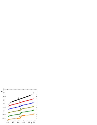
Figure 5: (Colour online) The chemical potential (in units of the nearest neighbour interaction energy $J$) versus concentration at $\beta J=0.3$ (1); 0.5 (2); 0.6 (3); 0.7 (4); 0.8 (5) and 1.0 (6). The solid lines represent the QChA results, the full circles are the MC simulation data. Each group of curves is shifted down by 10 units along the $\mu$ axis with respect to the previous one for better visibility. The unshifted curve (3) is characterized by $\mu/J=4$ at $c=0.5$, and this point is the same for all the temperatures. Thus, the groups of curves (1) and (2) are shifted up from their true position, while (4), (5) and (6) are shifted down. The same curves numbers are kept in figures 6–8.

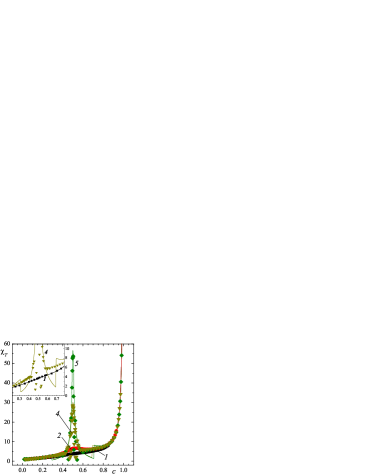
Figure 6: (Colour online) The thermodynamic factor versus concentration at $\beta J=0.3$ (1, square); 0.5 (2, circle); 0.7 (4, down triangle) and 0.8 (5, diamond). The solid lines represent the QChA results, the symbols are the MC simulation data.

The thermodynamic factor is inverse to the concentration fluctuations. The latter grow immediately after the transition from a disordered to an ordered state and then decrease systematically until concentration $0.5$ is reached when the most ordered state is possible. Physically, this means that concentration fluctuations are suppressed in the ordered states.

In QChA, the chemical potential and the thermodynamic factor were calculated by numerical differentiating of the free energy expression (3.6). However, such a differentiation of the chemical potential extracted from MC simulations may not be used. In this case, the thermodynamic factor can be calculated as the value inversely proportional to the mean square concentration fluctuations

$$\chi_{T}=\frac{\langle n\rangle}{\langle(n-\langle n\rangle)^{2}\rangle}.$$ (4.1)

The parameter $\chi_{T}$ plays an important role in describing the diffusion process in lattice fluids [16].

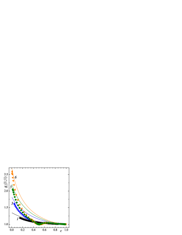
Figure 7: (Colour online) The correlation functions for nearest neighbours versus concentration at $\beta J=0.3$ (1, square); 0.6 (3, up triangle); 0.8 (5, diamond) and 1.0 (6, left-hand triangle). The solid lines represent the QChA results, the symbols are the MC simulation data.

The calculation and simulation results for the chemical potential and thermodynamic factor are in a good agreement except for those at close vicinity of the second order phase transition curve where the QChA curves show abrupt jumps.

A short range ordering is characterized by the correlation functions (3.14). These functions are more informative objects than the distribution functions because they represent the deviation of the short range correlations in interacting systems from the case of noninteracting (Langmuir) lattice gases where they are equal to one.

The correlation functions for nearest and next-next-nearest neighbours are show in figures 7 and 8, respectively.

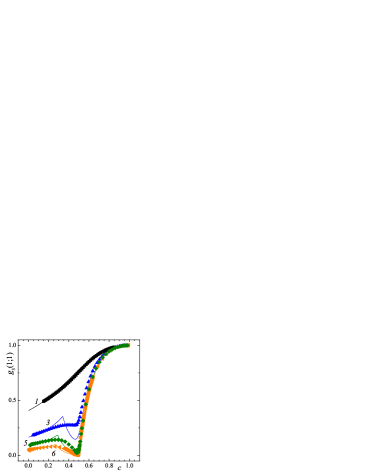
Figure 8: (Colour online) The correlation functions for the next-next-nearest neighbours versus concentration at $\beta J=0.3$ (1, square); 0.6 (3, up triangle); 0.8 (5, diamond) and 1.0 (6, left-hand triangle). The solid lines represent the QChA results, the symbols are the MC simulation data.

The long range ordering manifests itself in a short range structure as well. At temperatures $T<T_{\text{c}}$ (see curves 3, 5 and 6) the probability to find two next-next-nearest neighbour sites occupied by particles becomes very low. Of course, the higher is the temperature, the less pronounced difference from the Langmuir gas behaviour is observed.

The simulation and analytical results satisfactorily match each other in the disordered phase. They significantly differ at intermediate concentrations and at low temperatures due to the problems concerning the determination of the order parameter and the critical temperature in QChA. The most significant differences appear for the correlations on the nearest neighbour lattice sites.

5 Conclusion

The lattice system with an attractive interaction between nearest neighbours and repulsive interaction between next-next-nearest neighbours has been studied.

It is shown that the competing interactions lead to the order-disorder phase transitions. The order parameter $\delta c$ is used as the indicator of the second order phase transitions. With this parameter, it was established that the critical value of the interaction parameter is equal to $|J_{1}|/k_{\text{B}}T_{\text{c}}=0.655\pm 0.005$, and the phase diagram of the system was constructed.

The quasi-chemical approximation is found to be self-consistently constructed through the mean potentials that describe the interaction of a particle or a vacancy with its nearest and next-next-nearest neighbour lattice sites. The chemical potential, thermodynamic factor and correlation functions are determined both in the QChA and in the Monte Carlo simulations. The chemical potential demonstrates irregular behaviour in the phase transition region, while the thermodynamic factor indicates strong suppressing of fluctuations that are inherent to the ordered states of the system. The complicated behaviour of the correlation functions that reflects structural peculiarities of the system demonstrate a great importance of competing interactions.

The order parameter of the system $\delta c$ is determined in the QChA with significant errors. This leads to errors in determining the critical temperature of the system, which is overestimated by approximately 30%. As a result, the quasichemical approximation fails to reproduce the structural characteristics of the system with competing interactions. At the same time, the thermodynamic characteristics such as the chemical potential and the thermodynamic factor are determined in the quasi-chemical approximation with a sufficiently high accuracy.

Thus, the developed approach allows us to correctly describe the qualitative features of the structural properties of the systems with competing interactions, and can be used to quantify the thermodynamic characteristics of these systems.

Ukrainian 0

Ðiâíîâàæíi âëàñòèâîñòi ґðàòêîâî¿ ñèñòåìè ç ïîòåíöiàëîì âçàєìîäi¿ òèïó SALR íà êâàäðàòíié ґðàòöi: êâàçiõiìiчíå íàáëèæåííÿ ó ïîðiâíÿííi ç ñèìóëÿöiÿìè Ìîíòå Êàðëî ß.Ã. Ãðîäà${}^{\textsf{\footnotesize{\mbox{?}}}}$, Â.Ñ. Âiõðåíêî${}^{\textsf{\footnotesize{\mbox{?}}}}$, Ä. äi Êàïðiî${}^{\textsf{\footnotesize{\mbox{?}}}}$

             
${}^{\textsf{\footnotesize 1}}$ Áiëîðóñüêèé äåðæàâíèé òåõíîëîãiчíèé óíiâåðñèòåò, âóë. Ñâєðäëîâà, 13a, 220006 Ìiíñüê, Áiëîðóñü ${}^{\textsf{\footnotesize 2}}$ Äîñëiäíèöüêèé óíiâåðñèòåò íàóêè òà ëiòåðàòóðè Ïàðèæó, ChimieParisTech — CNRS, Iíñòèòóò õiìiчíèõ äîñëiäæåíü Ïàðèæó, Ïàðèæ, Ôðàíöiÿ

References

- [1] Stradner A., Sedgwick H., Cardinaux F., Poon W.C.K., Egelhaaf S.U., Schurtenberger P., Nature, 2004, 432, 492–495, doi:10.1038/Nature03109.
- [2] Khaldoun A., Moller P., Fall A., Wegdam G., De Leeuw B., Méheust Y., Fossum J.O., Bonn D., Phys. Rev. Lett., 2009, 103, 188301, doi:10.1103/PhysRevLett.103.188301.
- [3] Meyra A.G., Zarragoicoechea G.J., Kuz V.A., Phys. Rev. E, 2015, 91, 052810, doi:10.1103/PhysRevE.91.052810.
- [4] Archer A.J., Pini D., Evans R., Reatto L., J. Chem. Phys., 2007, 126, 014104, doi:10.1063/1.2405355.
-
[5]
Pini D., Jialin G., Parola A., Reatto L., Chem. Phys. Lett., 2000, 327, 209–215,
doi:10.1016/S0009-2614(00)00763-6. - [6] Pȩkalski J., Ciach A., Almarza N.G., J. Chem. Phys., 2014, 140, 114701, doi:10.1063/1.4868001.
- [7] Almarza N.G., Pȩkalski J., Ciach A., J. Chem. Phys., 2014, 140, 164708, doi:10.1063/1.4871901.
- [8] Groda Y., Bildanov E., Vikhrenko V., In: Proceedings of the 7th International Conference “Nanomaterials: Applications and Properties” (Odesa, 2017), IEEE, 2017, 03NNSA31, doi:10.1109/NAP.2017.8190275.
- [9] Uebing C., Gomer R., J. Chem. Phys., 1991, 95, 7641, doi:10.1063/1.461817.
- [10] Binder K., Landau D.P., Phys. Rev. B, 1980, 21, 1941–1963, doi:10.1103/PhysRevB.21.1941.
-
[11]
Groda Ya.G., Argyrakis P., Bokun G.S., Vikhrenko V.S., Eur. Phys. J. B, 2003, 32, 527–535,
doi:10.1140/epjb/e2003-00118-3. -
[12]
Groda Y.G., Lasovsky R.N., Vikhrenko V.S., Solid State Ionics, 2005, 176, 1675–1680,
doi:10.1016/j.ssi.2005.04.016. - [13] Bokun G.S., Groda Ya.G., Belov V.V., Uebing C., Vikhrenko V.S., Eur. Phys. J. B, 2000, 15, 297–304, doi:10.1007/s100510051128.
- [14] Domb C., Adv. Phys., 1960, 9, 149–244, doi:10.1080/00018736000101189.
- [15] Huang K., Statistical Mechanics, Wiley, New York, 1963.
-
[16]
Bokun G.S., Groda Ya.G., Uebing C., Vikhrenko V.S., Physica A, 2001, 296, 83–105,
doi:10.1016/S0378-4371(01)00163-7.
Ukrainian \adddialect\l@ukrainian0 \l@ukrainian