On Order Types of Random Point Sets

Abstract

A simple method to produce a random order type is to take the order type of a random point set. We conjecture that many probability distributions on order types defined in this way are heavily concentrated and therefore sample inefficiently the space of order types. We present two results on this question. First, we study experimentally the bias in the order types of $n$ random points chosen uniformly and independently in a square, for $n$ up to $16$. Second, we study algorithms for determining the order type of a point set in terms of the number of coordinate bits they require to know. We give an algorithm that requires on average $4n\log_{2}n+O(n)$ bits to determine the order type of $P$, and show that any algorithm requires at least $4n\log_{2}n-O(n\log\log n)$ bits. This implies that the concentration conjecture cannot be proven by an “efficient encoding” argument.

1 Introduction

An order type is a combinatorial abstraction of a finite point configuration that already determines which subsets are in convex position and which pairs define intersecting segments. (Hence, the order type of a point set $P$ encodes the convex hull, the convex pealing structure, the triangulations of $P$, or, for instance, which graphs admit straight-line embeddings with vertices mapped to $P$.) In this paper, we study the problem of producing random order types efficiently and with limited bias.

1.1 Context

The orientation of a triple $(a,b,c)\in({\mathbb{R}}^{2})^{3}$ is the sign of the determinant

$$\left|\begin{matrix}a_{x}&b_{x}&c_{x}\\ a_{y}&b_{y}&c_{y}\\ 1&1&1\end{matrix}\right|,\qquad\text{where $a_{x}$ is the $x$-coordinate of $a$, etc.}$$

This sign is $-1$ if the triangle $abc$ is oriented clockwise (CW), $0$ if it is flat, and $1$ if it is oriented counterclockwise (CCW). Two sequences $P=(p_{1},p_{2},\ldots,p_{n})\in({\mathbb{R}}^{2})^{n}$ and $Q=(q_{1},q_{2},\ldots,q_{n})\in({\mathbb{R}}^{2})^{n}$ have the same chirotope if for every indices $i,j,k$ the triples $(p_{i},p_{j},p_{k})$ and $(q_{i},q_{j},q_{k})$ have the same orientation. A related notion is for two finite subsets $P$ and $Q$ of ${\mathbb{R}}^{2}$ to have the same order type, meaning that there exists a bijection $f:P\to Q$ that preserves orientations. Having the same order type (resp. chirotope) is an equivalence relation, and an order type (resp. a chirotope) is an equivalence class for that relation. An order type or chirotope is simple if it can be realized without three collinear points. These definitions extend readily to ${\mathbb{R}}^{d}$, but we consider here only the planar, simple case.

Order types VS chirotopes.

The questions we are interested in are usually oblivious to the labeling of the points, and are therefore phrased in terms of order types. Our methods do, however, make explicit use of the labeling of the points, so our results are stated in terms of chirotopes for the sake of precision. We therefore use one or the other notion depending on the context. They are related since an order type of size $n$ corresponds to at most $n!$ chirotopes, possibly fewer if some bijections of the point set into itself preserve orientations.

Enumerating order types.

There are finitely many order types of size $n$, so, in principle, some properties of planar point sets of small size can be studied by sheer enumeration of order types. In practice, order types were enumerated (up to possible reflexive symmetry) up to size $11$ by Aichholzer et al. [1]. They used their database for instance to establish sharp bounds on the minimum and maximum numbers of triangulations on $10$ points, a very finite result that they could bootstrap into an asymptotic bound. The number of order types of size $n$ does, however, quickly become overwhelming as $n$ increases: it reaches billions already for $n=11$, and grows at least as $n^{3n+o(n)}$ since the number of chirotopes grows as $n^{4n+\Theta\left(\frac{n}{\log n}\right)}$ [2, Theorem 4.1]. It is thus unlikely that the order type database will be extended much beyond size $11$.

1.2 Questions

When dealing with configuration spaces too large to be enumerated, it is natural to fall back on random sampling methods. Two desirable properties of a random generator of order types are that it be efficient (a random order type can be produced quickly, say in time polynomial in $n$) and reasonably unbiased (it will explore a reasonably large fraction of the space of order types).

Challenges.

Designing an efficient and reasonably unbiased random generator of order types may prove difficult because of two properties of order types. On the one hand, order types enjoy small combinatorial encodings, even of subquadratic size [6], but the set of order types is difficult to describe: already deciding membership is NP-hard [14]. On the other hand, order types can be manipulated through point sets realizing them, so that one needs not worry about remaining in the space of order types, but there are order types of size $n$ for which any realization requires $2^{\Omega(n)}$ bits per coordinate [11].

Concentration.

Let us illustrate what we consider unreasonable bias. Let $m_{n}$ be a sequence of positive integers with $m_{n}\to\infty$, and let $\mu_{n}$ be a probability measure on the set of order types of size $m_{n}$. Say that $\{\mu_{n}\}_{n\in{\mathbb{N}}}$ exhibits concentration if there exists for each $n$ a set $S_{n}$ of order types of size $m_{n}$ such that $S_{n}$ contains a proportion $\epsilon_{n}\to 0$ of all order types, while $\mu_{n}(S_{n})\to 1$. In other words, $\mu_{n}$ and the counting measure on order types of size $m_{n}$ are “asymptotically singular”. In fact, little seems known already on the following question.

Open problem 1.

Does there exist a sequence of measures $\mu_{n}$ on order types of size $m_{n}$ such that (i) no subsequence exhibits concentration, and (ii) a random order type of size $m_{n}$ according to measure $\mu_{n}$ can be produced in time polynomial in $n$?

Random point sets.

It is easy to produce a random order type by first generating a random point set, then reading off its order type, but let us stress that it is not clear how the probability distribution on point sets translates into a probability distribution on order types.

Open problem 2.

How biased is the order type of a set of points sampled from a planar measure (say uniform on a square)?

When sampling points independently and from a probability distribution whose support has non-empty interior, every order type appears with positive probability. Indeed, every order type can be realized on an integer grid [11] and order types are unchanged under rescaling and sufficiently small perturbation. One may still expect some bias, if only because some order types require exponential precision for their realization [11] and are thus more brittle than others. For order types of small size, bias was proven to be unavoidable [10, Prop. 2].

1.3 Results

For the sake of clarity, we state and prove our results for a uniform sample of a square, understood as a sequence of random points chosen independently and uniformly in $[0,1]^{2}$ (the choice of which square does not affect the distribution). We comment in Section 6 to what extent our methods generalize. We write $\log$ to mean the logarithm of base $2$.

Experiments.

Our first contribution (Section 2) is some experimental evidence that sampling random point sets uniformly and independently in a square explores very inefficiently the space of order types for $n$ up to $16$. This prompts:

Conjecture 3.

Let $\mu_{n}$ denote the probability distribution on order types of size $n$ given by uniformly sampling a square. The sequence $\{\mu_{n}\}_{n\in{\mathbb{N}}}$ exhibits concentration.

Algorithms.

Recall that the number of chirotopes grows as $n^{4n+\Theta\left(\frac{n}{\log n}\right)}$. An “entropic” approach to proving (the chirotopal analogue of) Conjecture 3 could thus be to find an algorithm that reads off the chirotope of a uniform sample of a square using with high probability at most $cn\log n$ random bits, for some $c<4$. Formally, we consider a discrete model of computation (e.g., a Turing machine), not the real-RAM machine customary in computational geometry, where reading the coordinates has a cost (specifically, accessing the next bit in one of these strings has unit cost) and any other computation is considered free. A random point set is then given in the form of $2n$ infinite binary strings, one per point coordinate and we want to determine its chirotope efficiently most of the time. Our second contribution establishes that such an approach fails:

Theorem 4.

Let $P$ be a uniform sample of size $n$ in $[0,1]^{2}$.

• Any algorithm that determines the chirotope of $P$ reads on average at least $4n\log n-O(n\log\log n)$ coordinate bits.

• There exists an algorithm that determines the chirotope of $P$ by reading on average $4n\log n+O(n)$ coordinate bits.

We prove Theorem 4 in two steps. First, Section 3 answers the questions listed above for an arbitrary point set $P$ in terms of two statistics ($L$ and $U$) of that point set. Sections 4 and 5 then make a probabilistic analysis of these statistics for our random point sets.

Another approach.

Our proof of Theorem 4 (ii) uses a similar argument (namely Lemma 13) as the following result of Fabila-Monroy and Huemer [8]: with probability at least $1-O\left(n^{-\epsilon}\right)$, a uniform sample of a square of size $n$ can be rounded to the regular grid of step $n^{-3-\epsilon}$ without changing its chirotope. Can most chirotopes be realized on a $O\left(n^{3+\epsilon}\right)\times O\left(n^{3+\epsilon}\right)$ regular grid? A negative answer would prove Conjecture 3. Unfortunately, the best bounds that we are aware of, due to Caraballo et al. [5], do not settle this question: they only assert that the number of chirotopes of resolution $n^{-3-\epsilon}$ is at least $n^{3n-O(n\log\log n/\log n)}$, whereas the number of chirotopes is $n^{4n+\Theta\left(\frac{n}{\log n}\right)}$.

2 Experimental study of order types of random point sets

In this section, we probe experimentally the probability distribution of order types of uniform samples of a square. Note that the number of order types is about $28$ million for size 10, between $2.3$ and $4.7$ billion for size 11 (see Appendix A), and unknown for $n\geq 12$.

Setup.

Our first experiment is to produce a large number $N$ of point sets, stopping after each million samples to record the empirical distribution of order types. We repeated this experiment 80 times for size $10$ (for $N=1$ billion) and 20 times for size $11$ (for $N=450$ million). For size $12$, we ran out of memory before getting useful information (we used machines with 16 to 64 gigabytes of memory.)

It seems plausible that the expected number of samples needed to reach a repetition provides some insight on how concentrated that measure is; for comparison, this expectation is $\Theta(\frac{1}{\sqrt{k}})$ for a uniform measure on $k$ elements. We thus set up a second experiment where we produce point sets until we reach the first repetition of an order type. We repeated this experiment 10000 times for each size from $10$ to $14$, 5468 times for size $15$ and 1000 times for size $16$.

Due to lack of space, we defer the discussion of technical issues to Appendix A.

Data.

We present here synthetic views of our experimental results.

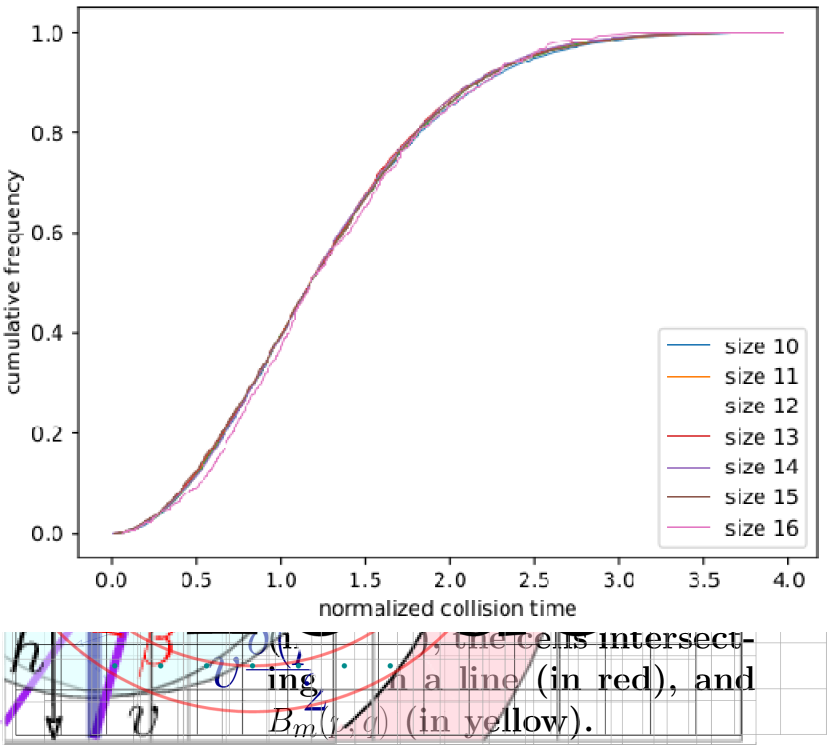
Figure 1: Results for the 1st experiment, averaged over 80 trials for size 10 and 20 trials for size 11. Left: Number of occurrences (average $\pm$ standard deviation) for the $k$th most frequent order types for $k=1,2,\ldots,1000$. Right: The proportion of new order types found (the scale is logarithmic on the $y$-axis). The table gives some triples $(x\%,s,d)$, meaning that after $s$ million samples, $d$ million distinct order types were found and $x\%$ of the last million samples were new ones.

Size	10	11	12	13	14	15	16
Average	466	2 716	18 788	156 372	1 521 365	17 134 843	218 060 427
Median	432	2 546	17 540	147 266	1 429 508	16 027 384	203 340 042

Table 1: Results for the 2nd experiment: time of first collision (averaged over 10 000 trials for size 10 to 14, 5468 for size 15 and 1000 for size 16).

Discussion.

For size 10 and 11, the empirical frequencies of the most popular order types are $5.6\ 10^{-4}$ and $7.3\ 10^{-5}$, which are several orders of magnitude above the corresponding uniform probability ($3.5\ 10^{-8}$ and about $4\ 10^{-10}$, respectively). This behavior persists, as even the 1000th popular order type remains $3$ to $4$ orders of magnitude more frequent than for the uniform behavior. Notice that (Figure 1 right) the rate at which new order types are discovered collapses quickly: for size 10, after seeing $\sim 2.2\ 10^{6}$ distinct order types, in the next million samples only $10\%$ produce a new order type; this means that $\sim 7.7\%$ of the order types of size 10 account for $90\%$ of the mass. The situation seems similar for size 11. Altogether, this suggests that uniform samples of a square explore very inefficiently the space of order types.

This first assessment may seem weakly justified as it is based on mere averages. We do not provide a statistical analysis of these estimators, but note that the random variable counting the number of distinct order types seen after $t$ samples is a sum of $t$ Bernoulli variables that are not independent, but are negatively associated in the sense explained in Section 5.2. This variable therefore enjoys a Chernoff-type tail estimate, and can be accurately estimated through averaging over a reasonably small number of samples. This is consistent with the rather small standard deviations observed on our samples. We thus believe that these empirical averages represent the situation quite fairly.

Our second experiment indicates that for size $12$ to $16$ the time of first collision remain orders of magnitude smaller than what it would be for a uniform distribution. Indeed, let us write $T_{n}$ for the number of order types of size $n$, and speculate on the value of $\sqrt{T_{n}}$ ($T_{n}$ is unknown for $n\geq 12$). For $n=10$ this is $5348$; the ratio $\frac{T_{n+1}}{T_{n}}$ increases regularly as $n$ ranges from $5$ to $10$, and is about $160$ for $n=10$. Assuming that it does not decrease, the value $\sqrt{T_{n}}$ should grow by a factor at least $12$, and likely much more. The average empirical first collision time grows by smaller factors: $5.8$, $6.9$, $8.3$, $9.7$, $11.2$ and $12.9$.

Let us sketch a more refined analysis. Let $p_{n,1},p_{n,2},\ldots,p_{n,T_{n}}$ denote the probabilities of the various order types in a random sample of a square, in non-increasing order. Let $\mu_{n}$ denote the probability distribution on $[T_{n}]$ such that $\mathbb{P}\left[\mu_{n}=i\right]=p_{n,i}$. Let $C_{\mu_{n}}$ denote the time of first collision for $\mu_{n}$ and let us identify $\mu_{n}$ to the vector $(p_{n,1},p_{n,2},\ldots,p_{n,T_{n}})$. Camarri and Pitman [4, Corollary 5] proved that $\frac{C_{\mu_{n}}}{\|\mu_{n}\|_{2}}$ asymptotically follows the Rayleigh distribution with density $x\exp(-x^{2}/2)$ if and only if $\|\mu_{i}\|_{\infty}=o\left(\|\mu_{i}\|_{2}\right)$. We found (by hand) a scaling of the times of first collision obtained experimentally so that their distribution seems to fit

that Rayleigh distribution (see figure on the right); a Kolmogorov-Smirnov test confirms that for $n=11$ to $16$, these normalized data are consistent with such a convergence. The hypothesis is asymptotic in nature and we only sampled order types up to size 16, but given that there are already billions of order types for size 11, this provides some (weak) evidence in favor of $\|\mu_{i}\|_{\infty}=o\left(\|\mu_{i}\|_{2}\right)$. Assuming this indeed holds, $\sqrt{2/\pi}C_{\mu_{n}}$ is an asymptotically unbiased estimator for $\|\mu_{i}\|_{2}$ (the constant factor comes from the mean of the Rayleigh distribution).

Does $\|\mu_{i}\|_{\infty}=o\left(\|\mu_{i}\|_{2}\right)$ relate to concentration? On one hand, it is compatible with $\mu_{i}$ being uniform on $i$ elements. On the other hand, if $\mu_{i}$ charges uniformly $n_{i}=o(i)$ elements for a total of $1-\frac{1}{i}$ and uniformly $i-n_{i}$ elements for a total of $\frac{1}{i}$, the condition is only satisfied for $n_{i}=\omega\left(\sqrt{i}\right)$. Perhaps this condition prevents too sharp a concentration.

3 Analysis of arbitrary point sets

We first introduce one algorithm and two statistics to analyze the information needed to determine the order type of an arbitrary set $P$ of $n$ points in the unit square, no three aligned.

Grids and orientations.

Let $G_{m}$ denote the partition of $[0,1]^{2}$ into $m\times m$ square cells of side length $\frac{1}{m}$ where the interior of each cell is of the form $\left(\frac{i}{m},\frac{i+1}{m}\right)\times\left(\frac{j}{m},\frac{j+1}{m}\right)$ with $0\leq i,j<m$. We often set $m=2^{k}$, so that knowing the first $k$ bits of both coordinates of a point amounts to knowing which cell of $G_{m}$ contains it. Remark that knowing three points up to $k$ bits (for each coordinate) suffices to determine their orientation if and only if the corresponding three cells of $G_{m}$ cannot be intersected by a line.

Greedy algorithm.

The algorithm that we propose for Theorem 4 (ii) refines greedily the coordinates of a point involved in a triangle with undetermined orientation, until the chirotope can be determined. We start with no bit read, so we only know that all points are in the unit square. At every step, we select one point and read one more bit for both of its coordinates. So, at every step of the algorithm, we know for each point some grid cell that contains it; the resolution of the grid may of course be different for every point. The selection is done greedily as follows:

Find three pairwise distinct indices $a,b,c$ such that the cells known to contain $p_{a}$, $p_{b}$, $p_{c}$ can be intersected by a line, and select one among these points known to the coarsest resolution.

We break ties arbitrarily, so this is perhaps a method rather than an algorithm. By definition, when the algorithm stops, the chirotope of $P$ can be determined from the precision at which every point is known. The algorithm does not stop if $P$ contains three aligned points.

Statistic $U$.

For $i\in[n]$, we define $U(i)$ as the smallest $k$ such that for any $a,b\in[n]\setminus\{i\}$, there does not exist a line that intersects the cells in $G_{2^{k}}$ that contain $p_{a}$, $p_{b}$, and $p_{i}$. If $p_{i}$ is aligned with some two other points of $P$, we let $U(i)=\infty$. The following implies that our greedy algorithm terminates if $P$ has no aligned triple.

Lemma 5.

In the greedy algorithm above, independently of how ties are resolved, for every $i\in[n]$, at most $U(i)$ bits are read from each coordinate of $p_{i}$.

Proof.

Assume that at some point in the algorithm, we read the $k$th bit of both coordinates of point $p_{i}$. To read these bits, our selection method requires that there exist $a,b\in[n]\setminus\{i\}$ such that (1) in $\{p_{a},p_{b},p_{i}\}$, $p_{i}$ is one of the points known at coarsest resolution, and (2) there exists a line intersecting the cells known to contain $p_{a}$, $p_{b}$, and $p_{i}$. Condition (1) ensures that for each of $\{p_{a},p_{b},p_{i}\}$, the cell known to contain the point is contained in a cell of $G_{2^{k-1}}$. Condition (2) ensures that these cells in $G_{2^{k-1}}$ can be intersected by a line. Thus, $k-1<U(i)$. ∎

Statistic $L$.

For $i\in[n]$, we define $L(i)$ as the smallest $k$ such that at least one horizontal or vertical segments of length $2^{-k}$ starting in $p_{i}$ is disjoint from all lines $p_{a}p_{b}$ with $a,b\in[n]\setminus\{i\}$.

Lemma 6.

Any algorithm that determines the chirotope of $P$ must read, for every $i$, at least $L(i)-1$ bits of each coordinate of $p_{i}$.

Proof.

Assume that we know $k$ bits of the $x$-coordinate of the point $p_{i}$. The set of possible positions for $p_{i}$ then contains a horizontal segment $S$ of length $2^{-k}$ containing $p_{i}$; in fact, it would be exactly such a segment if we knew the $y$-coordinate of $p_{i}$ to infinite precision.

By definition of $L(i)$, the two horizontal segments of length $2^{-(L(i)-1)}$ starting in $p_{i}$ both intersect some line $p_{a}p_{b}$ with $a,b\in[n]\setminus\{i\}$ (the lines are different for the two segments). If $2^{-k}\geq 2\cdot 2^{-(L(i)-1)}$, then the segment $S$ contains at least one of these horizontal segments, and is also intersected by some line $p_{a}p_{b}$ with $a,b\in[n]\setminus\{i\}$. Since the possible positions of $p_{i}$ contain $S$, this means that the bits read so far from $p_{i}$ do not suffice to determine the orientation of the triple $(p_{i},p_{a},p_{b})$, even if $p_{a}$ and $p_{b}$ were known to infinite precision.

Conversely, if an algorithm that determines the chirotope of $P$ reads $k$ bits from the $x$-coordinate of $p_{i}$, then we must have $2^{-k}<2\cdot 2^{-(L(i)-1)}$, that is $k>L(i)-2$. The same argument applies to the $y$-coordinate of $p_{i}$. ∎

From here…

So the minimal number of bits required to determine the chirotope of $P$ is in between $2\sum_{i=1}^{n}(L(i)-1)$ and $2\sum_{i=1}^{n}U(i)$. We show in the next sections that both sums equal, at first order, $4n\log n$ on average when $P$ is a uniform sample of the unit square.

4 Probabilistic analysis of $U$

We now outline an analysis of the random variable $U(\cdot)$ when $P$ is a uniform sample of the unit square. The variables $U(i)$ have the same distribution, which satisfies

Lemma 7.

$\mathbb{E}\left[U(1)\right]\leq 2\log n+8$

Given two points $p$ and $q$ in $[0,1]^{2}$, the butterfly $B_{m}(p,q)$ is the set of positions of a point $r\in[0,1]^{2}$ such that the cells of $G_{m}$ containing these three points do not determine the orientation of $(p,q,r)$. Formally, $B_{m}(p,q)$ is the union of all cells of $G_{m}$ that intersect a line secant to the cells of $G_{m}$ that contain $p$ and $q$. The random variable $U(i)$ equals the smallest $k$ such that $\bigcup_{j\neq i}B_{2^{k}}(p_{i},p_{j})$ contains no other point of $P$. We prove Lemma 7 by bounding from above the area of a butterfly in terms of $m$ and the distance $pq$ and applying a union bound. Fabila-Monroy and Huemer[8] introduced a very close notion of butterfly (c.f. their sets $F_{i,j}$) to study how rounding coordinates affects order types. They already performed the analysis we

need [8, Lemmas 3 and 4], so we only spell out the proof of Lemma 7 in Appendix B for completeness.

We can now prove that our greedy algorithm for deciding the chirotope of $P$ reads on average at most $4n\log n+O(n)$ coordinate bits.

Proof of Theorem 4 (ii).

By Lemma 5, our greedy algorithm reads at most $U(a)$ bits from each coordinate of point $p_{a}$. Thus, using Lemma 7, the average number of bits used by our algorithm is at most: $2\mathbb{E}\left[\sum_{i=1}^{n}U(i)\right]=2\sum_{i=1}^{n}\mathbb{E}\left[U(i)\right]=2n\mathbb{E}\left[U(1)\right]\leq 4n\log n+16n.$ ∎

5 Probabilistic analysis of $L$

We now outline an analysis of the random variable $L(\cdot)$ when $P$ is a uniform sample of the unit square. Again, the variables $L(i)$ have the same distribution. The key technical result is:

Lemma 8.

For every $x>1$, there exists $c>0$ such that $\mathbb{P}\left[L(1)\geq 2\log n-x\log\log n\right]$ is at least $1-2^{-cn}$.

Proving Lemma 8 will take the rest of the section, but let us start by using it.

Proof of Theorem 4 (i).

All $n$ variables $L(i)$ have the same expectation and by Lemma 6, any algorithm that determines the chirotope of $P$ must read at least a total of $2(\sum_{i}L(i)-1)$. It thus suffice to determine $\mathbb{E}\left[L(1)\right]$, which rewrites as $\mathbb{E}\left[L(1)\right]=\sum_{k\geq 0}\mathbb{P}\left[L(1)>k\right]$.

Note that $\mathbb{P}\left[L(1)>k\right]$ decreases with $k$. Lemma 8 for $x=\frac{3}{2}$ implies that the first $2\log n-\frac{3}{2}\log\log n$ terms are at least $1-2^{-cn}$ for some constant $c>0$. Keeping only these terms, we get

$$\mathbb{E}\left[L(1)\right]\geq(1-2^{-cn})\left(2\log n-\frac{3}{2}\log\log n\right)\geq(1-2^{-cn})2\log n-\frac{3}{2}\log\log n.$$

For $n$ large enough, $2^{-cn+1}\log n<\frac{1}{2}\log\log n$ and the statement follows. ∎

5.1 Discretization into a bichromatic birthday problem

Our approach is to look for lines passing close to $p_{1}$, as such lines are likely to force $L(1)$ to be large. To do so, we divide the plane into some number of angular sectors around $p_{1}$ and define a blue disk of center $p_{1}$ and radius $0.2$ and a red annulus with center $p_{1}$ and radii $0.3$ and $0.4$. This discretizes the problem, as if we find two points of $P$ in the blue and red parts of the same or nearby sectors, then they must span a line passing close to $p_{1}$.

One technical issue is that if $p_{1}$ is close enough to the boundary of $[0,1]^{2}$, then parts of the red and blue regions will be outside of $[0,1]^{2}$ and cannot contain any point of $P$. We handle this by considering the 4 diagonal directions $(\pm 1,\pm 1)$, and picking the one in which the boundary is the furthest away from $p_{1}$. Now, in the cone of half-angle $\pi/8$ around that direction, the red and blue parts are contained in the unit square. Letting $8s$ denote the total number of sectors, we therefore focus on the $s$ sectors around that direction. For the rest of this section, we assume that this direction is $(1,1)$ as illustrated by the figure; the three other cases are symmetric. We label $B_{1},B_{2},\ldots B_{s}$ (resp. $R_{1},R_{2},\ldots R_{s}$) the intersection of each of our angular sectors with the blue disk minus $p_{1}$ (resp. the red annulus), in counterclockwise order.

Next, finding a line close to $p_{1}$ is not enough: to ensure that $L(1)>k$, we need to find lines that intersect all four horizontal and vertical segments of length $2^{-k}$ with endpoint $p_{1}$. To do that, we look for lines $(br)$ where $b\in B_{i}$ and $r\in R_{i+1}$. This shift in indices ensures that the line $(br)$ is close to $p_{1}$ and passes below $p_{1}$: indeed, $r$ and $b$ are respectively above and below the ray from $p_{1}$ that is a common boundary of $B_{i}$ and $R_{i+1}$. Similarly, finding some points $b^{\prime}\in B_{i^{\prime}}$ and $r^{\prime}\in R_{i^{\prime}-1}$ will provide a line $(b^{\prime}r^{\prime})$ passing close to $p_{1}$ and above it; together, these two lines will intersect all four horizontal and vertical segments that have $p_{1}$ as an endpoint. It remains to relate the size of these segments to $s$.

Since we consider what happens around the direction $(1,1)$, the line passing below $p_{1}$ will have to intersect both the horizontal segment with $p_{1}$ as leftmost point and the vertical segment with $p_{1}$ as topmost point. Note, however, that any line $(br)$ that we consider has slope at least $\tan\frac{\pi}{8}=\sqrt{2}-1$. Let $\rightarrow_{\ell}$ and $\downarrow_{\ell}$ denote the segments of length $\ell$ with $p_{1}$ as, respectively, leftmost and topmost point. If a line $(br)$ intersects $\downarrow_{\ell}$, it must also intersect $\rightarrow_{\frac{\ell}{\sqrt{2}-1}}$. We thus focus on finding the smallest $\ell$ such that $\downarrow_{\ell}$ is guaranteed to meet $(br)$.

Lemma 9.

If $s\geq 10$, for any point $b\in B_{i}$ and $r\in R_{i+1}$, the line $(br)$ intersects $\downarrow_{\frac{\pi}{2s}}$.

Proof.

The proof involves elementary geometry and is deferred to Appendix C. ∎

Altogether, we can bound $L(1)$ from below by a simple balls-in-bins condition:

Corollary 10.

Assume that $k\geq 3$ and that $s=2^{k+1}$. If there exists $i,i^{\prime}$ in $[s]$ such that $P$ intersects each of the four regions $B_{i}$, $R_{i+1}$, $B_{i^{\prime}}$, and $R_{i^{\prime}-1}$, then $L(1)\geq k$.

Proof.

Let $b\in B_{i}\cap P$ and $r\in R_{i+1}\cap P$. Since $s\geq 16$, Lemma 9 ensures that the line $(br)$ intersects $\downarrow_{\frac{\pi}{2s}}$. As argued before Lemma 9, that line also intersects $\downarrow_{\ell}$ and $\rightarrow_{\ell}$ with $\ell=\frac{\pi}{2(\sqrt{2}-1)s}$. A symmetry with respect to the line of slope 1 through $p_{1}$ gives the intersection with the two other segments from the points in $B_{i^{\prime}}$ and $R_{i^{\prime}-1}$. Since $\frac{\pi}{2(\sqrt{2}-1)}\leq 4$, the existence of $i$ and $i^{\prime}$ ensures that all four horizontal and vertical segments of length $\frac{4}{s}=2^{-k+1}$ starting in $p_{i}$ are intersected by some lines spanned by $P\setminus\{p_{1}\}$, so $L(1)>k-1$. ∎

5.2 A balls-in-bins analysis

To prove Lemma 8, we are interested in the probability that $L(1)$ be at least $2n\log n$ (minus some change), so we use Corollary 10 with $s=\frac{n^{2}}{\log^{x}n}$ and $x>1$. To study the probability that the indices $i$ and $i^{\prime}$ exist, we define, for $i\in[s]$ and $j\in[n-1]$, the random variables

$X_{i,j}=\mathbb{1}_{p_{j+1}\in B_{i}}$	$X_{i}=\max_{j\in[n-1]}X_{i,j}$	$X=\sum_{i\in[s]}X_{i}$
$Y_{i,j}=\mathbb{1}_{p_{j+1}\in R_{i}}$	$Y_{i}=\max_{j\in[n-1]}Y_{i,j}$	$Y=\sum_{i\in[s]}Y_{i}$

(Note that, for a better bookkeeping, we index the events associated with $p_{j}$ by $j-1$ because $p_{1}$ is already chosen.) In plain English, $X_{i}$ is the indicator variable that $B_{i}$ is non-empty, and $X$ counts the number of non-empty regions $B_{i}$. (The $Y_{i}$ and $Y$ variables do the same for the regions $R_{i}$.) The definition of the regions ensures that each is fully contained in the unit square, that all $B_{i}$ have the same area, and that all $R_{i}$ have the same area. So all the $\{X_{i,j}\}_{i,j}$ are identically distributed, and so are the $\{Y_{i,j}\}_{i,j}$, the $\{X_{i}\}_{i}$, and the $\{Y_{i}\}_{i}$.

Approach.

Conditioning on $X=\beta$ and $Y=\rho$, there are $\beta$ or $\beta-1$ red cells whose index follows the index of an occupied blue cell (depending on $B_{s}$). Since the $\rho$ occupied red cells are chosen uniformly amongst the $s$ red cells, we get:

$$\mathbb{P}\left[\exists i\colon B_{i}\cap P\neq\emptyset\text{ and }R_{i+1}\cap P\neq\emptyset\mid X=\beta,Y=\rho\right]\geq 1-\left(1-\frac{\beta-1}{s}\right)^{\rho}.$$ (1)

Indeed, all but at most one of the occupied blue cells are next to a red cell which, if occupied, makes the event true. Our approach is to combine this inequality with a concentration bound for $X$ and $Y$ to bound from below the probability that $i$ exists. A symmetric argument takes care of the existence of $i^{\prime}$.

Concentration of sums of dependent variables.

If the $X_{i}$ and the $Y_{i}$ were independent, the Chernoff-Hoeffding would bound from below the values of $X$ and $Y$ with high probability. For fixed $j$, however, any subset of $\{X_{i,j}\}_{i}\cup\{Y_{i,j}\}_{i}$ sums to zero or one; These variables are thus “negatively” dependent in the sense that when one is $1$, the others must be $0$. Formally, they can be shown to be negatively associated. We do not elaborate on this notion here, but refer to the paper of Dubhashi and Ranjan [7] from which we highlight the following points:

• Any finite set of $0-1$ random variables that sum to $1$ is negatively associated [7, Lemma 8]. So, the set $\{X_{i,j}\}_{i}\cup\{1-\sum_{i}X_{i,j}\}$ is negatively associated.

• Any set of increasing functions of pairwise disjoint subsets of negatively associated random variables forms, again, a set of negatively associated random variables [7, Proposition 7]. Thus, each of the sets $\{X_{i,j}\}_{i}$, $\{Y_{i,j}\}_{i}$, $\{X_{i}\}_{i\in[s]}$, and $\{Y_{i}\}_{i\in[s]}$ consists of negatively associated random variables.

• The Chernoff-Hoeffding bounds apply to sums of any set of negatively associated random variables [7, Proposition 5].

Hence, applying [12, Theorem 4.2] for $\delta=\frac{1}{2}$ for instance yields the desired concentration:

$$\mathbb{P}\left[X\leq\frac{\mathbb{E}\left[X\right]}{2}\right]\leq 0.89^{\mathbb{E}\left[X\right]}\quad\text{and similarly }\quad\mathbb{P}\left[Y\leq\frac{\mathbb{E}\left[Y\right]}{2}\right]\leq 0.89^{\mathbb{E}\left[Y\right]}.$$

Computations.

(Due to space limitations, some computations are abridged here and presented in full details in Appendix C). Each $B_{i}$ has area $c_{1}/s$, and each $R_{i}$ has area $c_{2}/s$ with $c_{1}=\frac{\pi}{200}$ and $c_{2}=\frac{7\pi}{800}$. Thus, $X_{i,j}$ and $Y_{i,j}$ are $0-1$ random variables, taking value $1$ with probability, respectively, $c_{1}/s$ and $c_{2}/s$. For fixed $i$, the $\{X_{i,j}\}_{j\in[n-1]}$ are independent, so we have $\mathbb{E}\left[X_{i}\right]=c_{1}\frac{\log^{x}n}{n}-O\left(\frac{\log^{2x}n}{n^{2}}\right)$ and $\mathbb{E}\left[Y_{i}\right]\geq c_{2}\frac{\log^{x}n}{n}-O\left(\frac{\log^{2x}n}{n^{2}}\right)$. Since the $X_{i}$ are identically distributed, and so are the $Y_{i}$, we have

$$\mathbb{E}\left[X\right]=s\mathbb{E}\left[X_{i}\right]\geq c_{1}n-O\left(\log^{x}n\right)\quad\text{and}\quad\mathbb{E}\left[Y\right]=s\mathbb{E}\left[Y_{i}\right]\geq c_{2}n-O\left(\log^{x}n\right).$$

Now, let $\mathcal{O}$ denote the event that there exist $a,b$ in $[s]$ such that each of $B_{a}$, $R_{a+1}$, $B_{b}$, $R_{b-1}$ is hit by $P$. Let us condition by the event $\mathcal{G}=\{X\geq\mathbb{E}\left[X\right]/2\hbox{\ and\ }Y\geq\mathbb{E}\left[Y\right]/2\}$. A union bound yields

$$\mathbb{P}\left[\mathcal{G}\right]\geq 1-\left(0.89^{\mathbb{E}\left[X\right]}+0.89^{\mathbb{E}\left[Y\right]}\right)\geq 1-\left(0.89^{c_{1}n-O\left(\log^{x}n\right)}+0.89^{c_{2}n-O\left(\log^{x}n\right)}\right)$$

which is exponentially close to $1$. We thus bound from below $\mathbb{P}\left[\mathcal{O}\right]\geq\mathbb{P}\left[\mathcal{G}\right]\mathbb{P}\left[\mathcal{O}|\mathcal{G}\right]$ and concentrate on the conditional probability.

Bichromatic birthday paradox.

(Due to space limitations, some computations are abridged here and presented in full details in Appendix C). The probability $\mathbb{P}\left[\mathcal{O}|\mathcal{G}\right]$ can be expressed as a convex combination of the conditional probabilities $f(\beta,\rho)=\mathbb{P}\left[\mathcal{O}|\mathcal{G}_{\beta,\rho}\right]$, where for integers $\beta\geq\mathbb{E}\left[X\right]/2$ and $\rho\geq\mathbb{E}\left[Y\right]/2$ we take $\mathcal{G}_{\beta,\rho}=\{X=\beta,Y=\rho\}$. Conditioned on $\mathcal{G}_{\beta,\rho}$, the occupied regions of each type are uniformly random and independent, which simplifies the analysis. Furthermore, the function $f(\beta,\rho)$ is increasing in both variables (the more occupied regions there are, the more likely it is that the collisions we desire occur). Thus, we concentrate on finding a lower bound on $f(\beta,\rho)$ for $\beta=\left\lceil\frac{\mathbb{E}\left[X\right]}{2}\right\rceil$ and $\rho=\left\lceil\frac{\mathbb{E}\left[Y\right]}{2}\right\rceil$.

Assume the $\beta$ occupied blue regions have been chosen. Let $T_{+}$ (resp. $T_{-}$) denote the set of red regions in sectors following counterclockwise (resp. clockwise) the sectors whose blue regions have been chosen. Since the blue regions in the boundary angular sectors may be among those chosen, we have $\beta-1\leq|T_{+}|,|T_{-}|\leq\beta$. We now pick the $\rho$ red regions to be occupied. Let $E_{+}$ (resp. $E_{-}$) denote the event that a region of $T_{+}$ (resp. $T_{-}$) has been chosen among the $\rho$ red regions. Pretend, for the sake of the analysis, that we choose the red regions one by one. If none of the first $i$ regions chosen is in $T_{+}$, then next one has to be picked from the $s-i$ unpicked regions, at least $\beta-1$ of which are in $T_{+}$. Thus,

$$1-\mathbb{P}\left[E_{+}\right]\leq\prod_{i=0}^{\rho-1}\left(1-\frac{\beta-1}{s-i}\right)=\frac{(s-\rho)!(s-\beta+1)!}{s!(s-\beta-\rho+1)!}$$

Using a symmetric argument for $T_{-}$ and applying a union bound, we get $1-f(\beta,\rho)\leq 2\ \frac{(s-\rho)!(s-\beta+1)!}{s!(s-\beta-\rho+1)!}$. Note that for $\beta=\left\lceil\frac{\mathbb{E}\left[X\right]}{2}\right\rceil$ and $\rho=\left\lceil\frac{\mathbb{E}\left[Y\right]}{2}\right\rceil$, both $\beta$ and $\rho$ are $\Theta(n)=o(s)$. Taking logarithm and using Simpson’s approximation formula, which asserts that $\log(N!)=N\log(N)-N+O(\log N)$, we get

$$\log(1-f(\beta,\rho)) =s\log\left(1+\frac{\rho(\beta-1)}{s(s-\beta-\rho+1)}\right)-\rho\log\left(1+\frac{\beta-1}{s-\beta-\rho+1}\right)$$

$$\hskip 136.5733pt-\beta\log\left(1+\frac{\rho}{s-\beta-\rho+1}\right)+O\left(\log s\right).$$

Now in the regime we are looking at, we have $\beta=c_{1}n/2-O\left(\log^{x}n\right)$, $\rho=c_{2}n/2-O\left(\log^{x}n\right)$, and $s=\frac{n^{2}}{\log^{x}n}$. Taking first order Taylor expansions, our bound rewrites as

$$\log(1-f(\beta,\rho))=-\frac{\rho\beta}{s-\beta-\rho+1}+O(\log s)=-\frac{c_{1}c_{2}}{4}\log^{x}n+O\left(\log n\right).$$

provided we have $x>1$. Hence, $f(\beta,\rho)=1-\exp(\Theta(\log(n)^{x}))$. Altogether, we get that $\mathbb{P}\left[\mathcal{O}|\mathcal{G}\right]$ is exponentially close to $1$. Since $\mathbb{P}\left[\mathcal{G}\right]$ is also exponentially close to $1$, we finally get that our event $\mathcal{O}$ holds with probability exponentially close to $1$. With Corollary 10, this proves Lemma 8.

6 Extension to more general measures

We stated and proved our main result (Theorems 4) for a uniform sample of the unit square. The careful reader may observe, however, that we have taken care to separate the geometric from the probabilistic arguments. Although the multiplicative constants of the leading terms in the end-results matter (we want both $\mathbb{E}\left[U(i)\right]$ and $\mathbb{E}\left[L(i)\right]$ to equal $2\log n$ at first order), the multiplicative constants in the geometric arguments do not matter:

• In the analysis of $U$, if Lemma 12 (in appendix) is degraded from $\frac{6}{m}+\frac{4}{m\delta(p,q)}$ to $O(\frac{1}{m\delta(p,q)})$, the statement in Lemma 7 remains that $\mathbb{E}\left[U(1)\right]\leq 2\log n+O(1)$.

• If the blue disk and red annulus are scaled by a constant factor, Lemma 9 still holds with $\downarrow_{\frac{\pi}{2s}}$ replaced by $\downarrow_{\Theta\left(\frac{1}{s}\right)}$; this changes the choice of $s$ in Section 5.2 to $s=\Theta\left(\frac{n^{2}}{\log^{x}n}\right)$, which changes only at which exponential speed the probability that $L(1)\geq 2\log n-O(\log\log n)$ converges to $1$.

• More generally, the lower bound on $L(1)$ should work for any probability measure for which one can prove a uniform lower bound of $\Omega(1/s)$ for the probabilities of the individual blue and red regions.

It should therefore be clear that the same analysis, with different constants, holds for a variety of more general probability distributions for the points; examples include the uniform distribution on any bounded convex domain with non-empty interior, or even any distribution on such a convex set with a density that is bounded away from $0$.

Appendix A Experimental setup

We explain here in more detail how we conducted our experiments.

Signature.

We keep track of the order types already seen by storing them explicitly in the form of a signature word. Let $P$ be a set of $n$ points. For a labelling $\sigma$ of $P$ by $1,2,\ldots,n$, let

$$w(\sigma)=2a_{1,1}a_{1,2}\ldots a_{1,n-2}1a_{2,1}a_{2,2}\ldots a_{2,n-2}1a_{3,1}a_{3,2}\ldots a_{3,n-2}\ldots 1a_{n,1}a_{n,2}\ldots a_{n,n-2}$$

where $1a_{i,1},a_{i,2},\ldots$ are the labels of the points in circular counterclockwise (CCW) order around the $i$th point, starting from the first point (or from the second point when turning around the $1$st point). We define as signature of $P$ the word $w(\sigma)$ that is lexicographically smallest among the labelings $\sigma$ where the points labelled $1$ and $2$ are consecutive on the convex hull (in CCW order). The fact that this signature characterizes the order type of $P$ follows from Bokowski’s study of hyperline sequences [3, $\mathsection 1.6$].

Lemma 11.

Given a set of permutations of $n$ elements $\{\tau_{i}\}_{1\leq i\leq n}$ with $\tau_{1}(1)=2$ and $\tau_{i}(1)=1$ for $i>2$ obtained as the signature of a point set $P$, the orientation of a triple $(p_{a},p_{b},p_{c})$ with $a<b<c$ depends only on the comparison of $\tau_{a}(b)$ and $\tau_{a}(c)$.

Proof.

The ambiguity comes from the fact that when we sort points around $p_{a}$ the angle $\widehat{p_{b}p_{a}p_{c}}$ may be greater or smaller than $\pi$. Up to an affine transformation, we may assume that for a realization of the order type: $p_{1}$ is the origin, $p_{2}=(0,-1)$, and $p_{a}=(x_{a},0)$. Then, since $p_{1}p_{2}$ is the edge of the convex hull after $p_{1}$ in counter-clockwise direction we get that $\forall 2<j<a,x_{j}>0,y_{j}<0$ and $\forall j>a,x_{j}>0,y_{j}>0$. In particular the angle $\widehat{p_{b}p_{a}p_{c}}\leq\pi$ and we deduce $\tau_{a}(b)<\tau_{a}(c)\Longleftrightarrow{\rm orient}(p_{a},p_{b},p_{c})={\tt ccw}$. ∎

Actually the above lemma allows to reduce the signature from an element of $[1,n]^{(n-1)\times n}$ to an element of $[3,n]^{n-2}\times[3,n]^{n-2}\times[4,n]^{n-3}\times\ldots\times[i,n]^{n-i+1}\times\times\ldots\times[n-1,n]^{2}$ reducing approximatively the signature size by a factor of 2. The signature, as well as its reduced form, can be computed in time $O(n^{3})$ in a straightforward way. The geometric computations are done using CGAL’s Exact_predicates_inexact_constructions_kernel [15].)

Pseudorandomess and precision.

We generated our point sets by picking the coordinates of each point in $[1.0,2.0]$. We used the pseudo-random generators of the standard C++ library, specifically we produce each point’s coordinate by a call to dis(gen) with:

• std::random_device rd;

• std::mt19937_64 gen(rd());

• std::uniform_real_distribution<double> dis(1.0, 2.0);

As a consequence, the precision is the same everywhere in the domain we sample, and every coordinate is given with $52$ bits of precision. Note that every order type of size $11$ can be represented exactly with $16$ bits of precision per coordinate [1].

Order types of size $10$ and $11$.

Aichholzer et al. [1] enumerated the order types up to size $11$. Their count is, however, up to reflection: they identify the order type of a point set with the order type of the reflection of that point set with respect to a line. For size up to $10$, they also readily provide realizations.  We examined every realization of size $10$ in their database and checked whether reflecting the points (horizontally) yields the same order type; this happened for $13\,064$ of the realizations. So, the total number of order types of size $10$ is $28\,606\,030$. We haven’t yet done this for size $11$, so we can only state that their number is between $2\ 334\ 512\ 907$ and twice that number. If the small number of symmetric order types of size $10$ is indicative, we should expect that the number of order types of size $11$ to be about $4.6$ billion.

Appendix B Analysis of $U(1)$ for a uniform sample of the unit square

Recall that $P$ is a uniform sample of the unit square of size $n$, and $G_{m}$ is the partition of $[0,1]^{2}$ into $m\times m$ square cells of side length $\frac{1}{m}$.

B.1 Butterflies

Given two points $p,q\in[0,1]^{2}$, we first let $B$ be the union of all lines intersecting the cells of $G_{m}$ containing $p$ and $q$; we then define $B_{m}(p,q)$ as the intersection of

$[0,1]^{2}$ with the Minkowski sum of $B$ with a disk of radius $\frac{\sqrt{2}}{m}$. We call $B_{m}(p,q)$ the butterfly of $p$ and $q$ (at resolution $m$). Note that the butterfly $B_{m}(p,q)$ contains all the cells intersecting $B$. Hence, if there exists a line intersecting the cells of $p$, $q$ and $r$, then $r\in B_{m}(p,q)$. The following lemma bounds the area of $B_{m}(p,q)$ by $O(\frac{1}{m\delta(p,q)})$.

Lemma 12.

The area of $B_{m}(p,q)$ is at most $\frac{6}{m}+\frac{4}{m\delta(p,q)}$ where $\delta(p,q)$ is the distance between the centers of the cells of $p$ and $q$.

Proof.

This lemma is similar to Lemma 3 in Fabila-Monroy and Huemer paper [8], although their analogous of butterfly have different definition. Note that the bound holds trivially if $p$ and $q$ are in the same cell ($\delta(p,q)=0$) or in adjacent cells ($\delta(p,q)=1/m$). Otherwise, the butterfly $B_{m}(p,q)$ consists of two parts: a strip $S_{m}(p,q)$ and the union $T_{m}(p,q)$ of four triangles (shaded in, respectively, green and blue in the figure). We have

$$\operatorname{area}\left(S_{m}(p,q)\right)\leq\left(3\frac{\sqrt{2}}{m}\right)\cdot\sqrt{2}=\frac{6}{m}.$$

The four triangles come in two pairs of homothetic triangles, intersected with $[0,1]^{2}$. Each homothetic pair consists of images under scaling of a triangle whose basis is the half diagonal of a cell of length $\frac{\sqrt{2}}{2m}$ and whose height $h$ is at least $\frac{\delta(p,q)}{2\sqrt{2}}$ (the two kinds of triangles have blue and red boundaries in the figure). Letting $u$ and $v$ denote the scaling

factors, the areas of the two homothetic triangles sum to $\frac{1}{2}(u^{2}+v^{2})h\frac{\sqrt{2}}{2m}$. Since the scalings turn the height of the reference triangles to two lengths that sum to at most $\sqrt{2}$, we have $(u+v)h\leq\sqrt{2}$. This implies that $u^{2}+v^{2}\leq\left(\frac{\sqrt{2}}{h}\right)^{2}$ and one pair of homothetic triangles contributes at most $\frac{1}{2}\frac{2}{h^{2}}h\frac{\sqrt{2}}{2m}=\frac{\sqrt{2}}{2hm}\leq\frac{2}{m\delta(p,q)}$. Altogether, $\operatorname{area}\left(T_{m}(p,q)\right)\leq\frac{4}{m\delta(p,q)}$. Finally $\operatorname{area}\left(B_{m}(p,q)\right)\leq\frac{6}{m}+\frac{4}{m\delta(p,q)}.$ ∎

B.2 Distribution of $U(1)$

We now analyze the distribution function of the random variable $U(1)$. Recall that the randomness here refers to the choice of the random points $p_{1},p_{2},\ldots p_{n}$, which are taken independently and uniformly in $[0,1]^{2}$.

Lemma 13.

$\mathbb{P}\left[U(1)>k\right]\leq 57n^{2}2^{-k}$.

Proof.

This lemma is similar to Lemma 4 in Fabila-Monroy and Huemer paper [8]. In our setting, we have:

$$\mathbb{P}\left[U(1)>k\right] \leq \mathbb{P}\left[\exists i,j\in\binom{[n]\setminus\{1\}}{2}:p_{j}\in B_{2^{k}}(p_{1},p_{i})\right]$$

$$\leq (n-1)\mathbb{P}\left[\exists j\in[n]\setminus\{1,2\}:p_{j}\in B_{2^{k}}(p_{1},p_{2})\right]$$

$$\leq (n-1)\mathbb{E}\left[1-(1-\operatorname{area}\left(B_{2^{k}}(p_{1},p_{2})\right))^{n-2}\right].$$

The geometry of $B_{2^{k}}(p_{1},p_{2})$ depends on the distance between the centers of the cells that contain $p_{1}$ and $p_{2}$. We therefore condition on the cell containing $p_{1}$, then sum the contributions of the cell containing $p_{2}$ by distance to the cell containing $p_{1}$. Accounting for boundary effects, for any $1\leq t\leq 2^{k}$ there are at most $8t$ cells whose center lies at a distance between $t2^{-k}$ and $(t+1)2^{-k}$ from a given cell. We thus have (using Lemma 12)

$$\mathbb{E}\left[1-(1-\operatorname{area}B_{2^{k}}(p_{1},p_{2}))^{n-2}\right]$$

$$= \sum_{c\in\text{ cells of }G_{2^{k}}}\mathbb{P}\left[p_{2}\in c\right]\cdot\mathbb{E}\left[1-(1-\operatorname{area}B_{2^{k}}(p_{1},p_{2}))^{n-2}\mid p_{2}\in c\right]$$

$$\leq \sum_{t=1}^{2^{k}}\frac{8t}{(2^{k})^{2}}\left(1-\left(1-\left(\frac{6}{2^{k}}+\frac{4}{2^{k}\cdot(t2^{-k})}\right)\right)^{n-2}\right).$$

Using $(1-x)^{n-2}\geq 1-(n-2)x$ we get

$$\mathbb{E}\left[1-(1-\operatorname{area}B_{2^{k}}(p_{1},p_{2}))^{n-2}\right] \leq (n-2)2^{-2k}\sum_{t=1}^{2^{k}}8t\left(6\cdot 2^{-k}+\frac{4}{t}\right)$$

$$\leq n2^{-2k}\left(\sum_{t=1}^{2^{k}}48t2^{-k}\right)+n2^{-2k}2^{k}32$$

$$\leq 24n2^{-k}(1+2^{-k})+32n2^{-k}.$$

The statement trivially bounds a probability by something greater than 1 for $k\leq 5$. For $k\geq 6$, the final term is at most $57n2^{-k}$. ∎

Lemma 7.

$\mathbb{E}\left[U(1)\right]\leq 2\log n+8$

Proof.

By definition we have

$$\mathbb{E}\left[U(1)\right]=\sum_{k=1}^{\infty}k\mathbb{P}\left[U(1)=k\right]=\sum_{k=0}^{\infty}\mathbb{P}\left[U(1)>k\right].$$

For the first $2\log n+6$ terms, we use the trivial upper bound of $1$ and for the remaining terms we use the upper bound of Lemma 13:

$$\mathbb{E}\left[U(1)\right]\leq(2\log n+6)+57n^{2}\sum_{k\geq 6+2\log n}^{\infty}2^{-k}=(2\log n+6)+57n^{2}\cdot 2^{-5-2\log n}.$$

Altogether it comes that $\mathbb{E}\left[U(1)\right]\leq 2\log n+8$. ∎

Appendix C Detailed proofs for Section 5

Lemma 9.

If $s\geq 10$, for any point $b\in B_{i}$ and $r\in R_{i+1}$, the line $(br)$ intersects $\downarrow_{\frac{\pi}{2s}}$.

Proof.

The vertical distance between $p_{1}$ and $(br)$ is maximal when $b$ and
$r$ are placed in the corners of $B_{s-1}$ and $R_{s}$ on circles of radii 0.2 and 0.3 as in left figure. Let us relate this maximal distance $h$ to $\theta=\widehat{bp_{1}r}$. With the notations of the right figure, considering triangle $vp_{1}b$ we have $\beta+\gamma+(\frac{7\pi}{8}-\theta)=\pi$ and deduce $\theta=\beta+\gamma-\frac{\pi}{8}$. Law of sines in the same triangle give $\sin\beta=\frac{pr}{vr}\sin\frac{7\pi}{8}=\frac{0.3}{\sqrt{0.09+h^{2}+0.6h\sin\frac{\pi}{8}}}\sin\frac{\pi}{8}$ and $\sin\gamma=\frac{h}{pb}\sin\beta=\frac{h}{0.2}\sin\beta$. And we can express $\theta$ as a function of $h$ (for $\theta$ sufficiently small):  

$$\theta=\arcsin\left(\tfrac{0.3}{\sqrt{0.09+h^{2}+0.6h\sin\tfrac{\pi}{8}}}\sin\tfrac{\pi}{8}\right)+\arcsin\left(\tfrac{0.3}{\sqrt{0.09+h^{2}+0.6h\sin\tfrac{\pi}{8}}}\tfrac{h}{0.2}\sin\tfrac{\pi}{8}\right)-\tfrac{\pi}{8}.$$

This function $h\mapsto\theta(h)$ is increasing on $[0,0.6]$ and $\theta(h)>h$ when $\theta(h)\in[0,0.17]$. Since $\theta$ is the angle of two sectors, we have $\theta=2\frac{\pi}{4s}$. For $s\geq 10$ we have $h<\frac{\pi}{2s}$. ∎

Computations.

Each $B_{i}$ has area $c_{1}/s$, and each $R_{i}$ has area $c_{2}/s$ with $c_{1}=\frac{\pi}{200}$ and $c_{2}=\frac{7\pi}{800}$. Thus, $X_{i,j}$ and $Y_{i,j}$ are $0-1$ random variables, taking value $1$ with probability, respectively, $c_{1}/s$ and $c_{2}/s$. For fixed $i$, the $\{X_{i,j}\}_{j\in[n-1]}$ are independent, so we have

$$\mathbb{E}\left[X_{i}\right]=\mathbb{P}\left[X_{i}=1\right]=1-\left(1-\frac{c_{1}}{s}\right)^{n-1}\geq 1-e^{-c_{1}\frac{n-1}{s}} \geq c_{1}\frac{n-1}{s}-\frac{1}{2}\left(c_{1}\frac{n-1}{s}\right)^{2}$$

$$=c_{1}\frac{\log^{x}n}{n}-O\left(\frac{\log^{2x}n}{n^{2}}\right).$$

the first and second inequalities coming, respectively, from the facts that for every $t\geq 0$ we have $1-t\leq e^{-t}$ and for every $t\in[0,1]$ we have $1-e^{-t}\geq-t-\frac{t^{2}}{2}$. Then, we plugged in $s=\frac{n^{2}}{\log^{x}n}$. The same computation gives $\mathbb{E}\left[Y_{i}\right]\geq c_{2}\frac{\log^{x}n}{n}-O\left(\frac{\log^{2x}n}{n^{2}}\right).$ Finally, since the $X_{i}$ are identically distributed, and so are the $Y_{i}$, we have

$$\mathbb{E}\left[X\right]=s\mathbb{E}\left[X_{i}\right]\geq c_{1}n-O\left(\log^{x}n\right)\quad\text{and}\quad\mathbb{E}\left[Y\right]=s\mathbb{E}\left[Y_{i}\right]\geq c_{2}n-O\left(\log^{x}n\right).$$

Now, let $\mathcal{O}$ denote the event that there exist $a,b$ in $[s]$ such that each of $B_{a}$, $R_{a+1}$, $B_{b}$, $R_{b-1}$ is hit by $P$. Let us condition by the event $\mathcal{G}=\{X\geq\mathbb{E}\left[X\right]/2\hbox{\ and\ }Y\geq\mathbb{E}\left[Y\right]/2\}$. A union bound yields

$$\mathbb{P}\left[\mathcal{G}\right]\geq 1-\left(0.89^{\mathbb{E}\left[X\right]}+0.89^{\mathbb{E}\left[Y\right]}\right)\geq 1-\left(0.89^{c_{1}n-O\left(\log^{x}n\right)}+0.89^{c_{2}n-O\left(\log^{x}n\right)}\right)$$

which is exponentially close to $1$. We thus bound from below $\mathbb{P}\left[\mathcal{O}\right]\geq\mathbb{P}\left[\mathcal{G}\right]\mathbb{P}\left[\mathcal{O}|\mathcal{G}\right]$ and concentrate on the conditional probability.

Bichromatic birthday paradox.

The probability $\mathbb{P}\left[\mathcal{O}|\mathcal{G}\right]$ can be expressed as a convex combination of the conditional probabilities $f(\beta,\rho)=\mathbb{P}\left[\mathcal{O}|\mathcal{G}_{\beta,\rho}\right]$, where for integers $\beta\geq\mathbb{E}\left[X\right]/2$ and $\rho\geq\mathbb{E}\left[Y\right]/2$ we take $\mathcal{G}_{\beta,\rho}=\{X=\beta,Y=\rho\}$. Conditioned on $\mathcal{G}_{\beta,\rho}$, the occupied regions of each type are uniformly random and independent, which will simplify the analysis. Furthermore, the function $f(\beta,\rho)$ is increasing in both variables (the more occupied regions there are, the more likely it is that the collisions we desire occur). Thus, we concentrate on finding a lower bound on $f(\beta,\rho)$ for $\beta=\left\lceil\frac{\mathbb{E}\left[X\right]}{2}\right\rceil$ and $\rho=\left\lceil\frac{\mathbb{E}\left[Y\right]}{2}\right\rceil$.

Assume the $\beta$ occupied blue regions have been chosen. Let $T_{+}$ (resp. $T_{-}$) denote the set of red regions in sectors following counterclockwise (resp. clockwise) the sectors whose blue regions have been chosen. Since the blue regions in the boundary angular sectors may be among those chosen, we have $\beta-1\leq|T_{+}|,|T_{-}|\leq\beta$. We now pick the $\rho$ red regions to be occupied. Let $E_{+}$ (resp. $E_{-}$) denote the event that a region of $T_{+}$ (resp. $T_{-}$) has been chosen among the $\rho$ red regions. Pretend, for the sake of the analysis, that we choose the red regions one by one. If none of the first $i$ regions chosen is in $T_{+}$, then next one has to be picked from the $s-i$ unpicked regions, at least $\beta-1$ of which are in $T_{+}$. Thus,

$$1-\mathbb{P}\left[E_{+}\right]\leq\prod_{i=0}^{\rho-1}\left(1-\frac{\beta-1}{s-i}\right) =\frac{(s-\beta+1)(s-\beta)\ldots(s-\beta-\rho+2)}{s(s-1)\ldots(s-\rho+1)}$$

$$=\frac{(s-\rho)!(s-\beta+1)!}{s!(s-\beta-\rho+1)!}$$

Using a symmetric argument for $T_{-}$ and applying a union bound, we get

$$1-f(\beta,\rho)\leq 2\ \frac{(s-\rho)!(s-\beta+1)!}{s!(s-\beta-\rho+1)!}.$$

Note that for $\beta=\left\lceil\frac{\mathbb{E}\left[X\right]}{2}\right\rceil$ and $\rho=\left\lceil\frac{\mathbb{E}\left[Y\right]}{2}\right\rceil$, both $\beta$ and $\rho$ are $\Theta(n)=o(s)$. Taking logarithm and using Simpson’s approximation formula, which asserts that $\log(N!)=N\log(N)-N+O(\log N)$, we get

$$\log(1-f(\beta,\rho)) =s\log\frac{(s-\rho)(s-\beta+1)}{s(s-\beta-\rho+1)}-\rho\log\frac{s-\rho}{s-\beta-\rho+1}$$

$$\hskip 113.81102pt-\beta\log\frac{s-\beta+1}{s-\beta-\rho+1}+O\left(\log s\right)$$

$$=s\log\left(1+\frac{\rho(\beta-1)}{s(s-\beta-\rho+1)}\right)-\rho\log\left(1+\frac{\beta-1}{s-\beta-\rho+1}\right)$$

$$\hskip 136.5733pt-\beta\log\left(1+\frac{\rho}{s-\beta-\rho+1}\right)+O\left(\log s\right).$$

Now in the regime we are looking at, we have $\beta=c_{1}n/2-O\left(\log^{x}n\right)$, $\rho=c_{2}n/2-O\left(\log^{x}n\right)$, and $s=\frac{n^{2}}{\log^{x}n}$. Taking first order Taylor expansions, our bound rewrites as

$$\log(1-f(\beta,\rho))=-\frac{\rho\beta}{s-\beta-\rho+1}+O(\log s)=-\frac{c_{1}c_{2}}{4}\log^{x}n+O\left(\log n\right).$$

provided we have $x>1$. Hence, $f(\beta,\rho)=1-\exp(\Theta(\log(n)^{x}))$. Altogether, we get that $\mathbb{P}\left[\mathcal{O}|\mathcal{G}\right]$ is exponentially close to $1$. Since $\mathbb{P}\left[\mathcal{G}\right]$ is also exponentially close to $1$, we finally get that our event $\mathcal{O}$ holds with probability exponentially close to $1$. With Corollary 10, this proves Lemma 8.

References

- [1] Oswin Aichholzer, Franz Aurenhammer, and Hannes Krasser. Enumerating order types for small point sets with applications. Order, 19(3):265–281, 2002.
- [2] Noga Alon. The number of polytopes, configurations and real matroids. Mathematika, 33(1):62–71, 1986.
- [3] Jürgen Bokowski and Juergen G Bokowski. Computational Oriented Matroids: equivalence classes of matrices within a natural framework. Cambridge University Press, 2006.
- [4] Michael Camarri and Jim Pitman. Limit distributions and random trees derived from the birthday paradox with unequal probabilities. Electronic Journal of Probability, 5(2):1–18, 2000.
- [5] Luis E Caraballo, José-Miguel Díaz-Báñez, Ruy Fabila-Monroy, Carlos Hidalgo-Toscano, Jesús Leaños, and Amanda Montejano. On the number of order types in integer grids of small size. arXiv preprint arXiv:1811.02455, 2018.
- [6] Jean Cardinal, Timothy M. Chan, John Iacono, Stefan Langerman, and Aurélien Ooms. Subquadratic Encodings for Point Configurations. In Bettina Speckmann and Csaba D. Tóth, editors, 34th International Symposium on Computational Geometry (SoCG 2018), volume 99 of Leibniz International Proceedings in Informatics (LIPIcs), pages 20:1–20:14, Dagstuhl, Germany, 2018. Schloss Dagstuhl–Leibniz-Zentrum fuer Informatik. URL: http://drops.dagstuhl.de/opus/volltexte/2018/8733, doi:10.4230/LIPIcs.SoCG.2018.20.
- [7] Devdatt Dubhashi and Desh Ranjan. Balls and bins: A study in negative dependence. Random Structures and Algorithms, 13(2):99–124, 1998.
- [8] Ruy Fabila-Monroy and Clemens Huemer. Order types of random point sets can be realized with small integer coordinates. In XVII Spanish Meeting on Computational Geometry: book of abstracts, Alicante, June 26-28, pages 73–76, 2017.
- [9] Tobias Gerken. Empty convex hexagons in planar point sets. Discrete & Computational Geometry, 39(1-3):239–272, 2008.
- [10] Xavier Goaoc, Alfredo Hubard, Rémi de Joannis de Verclos, Jean-Sébastien Sereni, and Jan Volec. Limits of order types. In LIPIcs-Leibniz International Proceedings in Informatics, volume 34. Schloss Dagstuhl-Leibniz-Zentrum fuer Informatik, 2015.
- [11] Jacob E Goodman, Richard Pollack, and Bernd Sturmfels. The intrinsic spread of a configuration in . Journal of the American Mathematical Society, pages 639–651, 1990.
- [12] Rajeev Motwani and Prabhakar Raghavan. Randomized Algorithms. Cambridge University Press, 1995.
- [13] Mark Overmars. Finding sets of points without empty convex 6-gons. Discrete & Computational Geometry, 29(1):153–158, 2002.
- [14] Peter Shor. Stretchability of pseudolines is NP-hard. Applied Geometry and Discrete Mathematics-The Victor Klee Festschrift, 1991.
- [15] The CGAL Project. CGAL User and Reference Manual. CGAL Editorial Board, 4.14 edition, 2019. URL: https://doc.cgal.org/4.14/Manual/packages.html.