Resolving $B$-meson anomalies by flavor-dependent gauged symmetries $\displaystyle\prod_{i=1}^{3}U(1)_{B_{i}-L_{i}}$

Abstract

We propose a model with flavor dependent gauged symmetries of $\displaystyle\prod_{i=1}^{3}U(1)_{B_{i}-L_{i}}$ with $i$ the family indices. After formulating the renormalizable Yukawa Lagrangian, Higgs potential and kinetic term, we study the lepton sector based on a successful two-zero texture without introducing extra scalar bosons to avoid the dangerous Goldstone bosons. In particular, we discuss the muon related phenomenologies via additional neutral gauge bosons. In our numerical analysis, we explore the allowed parameter space, in which the anomaly of $B\to K^{*}\bar{\mu}\mu$ can be explained.

I Introduction

Recently, there have been some anomalies in semi-leptonic $B$-meson decays Aaij:2014ora ; Aaij:2017vbb ; Aaij:2015esa ; Khachatryan:2015isa ; Lees:2015ymt ; Wei:2009zv ; Aaltonen:2011ja ; Aaij:2015oid ; Wehle:2016yoi ; Sirunyan:2017dhj ; Lees:2013uzd ; Aaij:2015yra , which would be hints of new physics (NP) beyond the standard model (SM) Hurth:2016fbr ; DAmico:2017mtc ; Altmannshofer:2017yso ; Hiller:2017bzc ; Geng:2017svp ; Ciuchini:2017mik ; Celis:2017doq ; Hurth:2017hxg ; Capdevila:2017bsm . For example, the ratio of $R_{K^{*}}\equiv{\cal B}(B^{0}\to K^{*0}\mu^{+}\mu^{-})/{\cal B}(B^{0}\to K^{*0}e^{+}e^{-})$ has been measured to be Aaij:2017vbb

$$R_{K^{*}}^{\rm expt} = \left\{\begin{array}[]{cc}0.66^{+0.11}_{-0.07}~{}{\rm(stat)}\pm 0.03~{}{\rm(syst)}~{},{}{}&0.045\leq q^{2}\leq 1.1~{}{\rm GeV}^{2}~{},\\ 0.69^{+0.11}_{-0.07}~{}{\rm(stat)}\pm 0.05~{}{\rm(syst)}~{},{}{}&1.1\leq q^{2}\leq 6.0~{}{\rm GeV}^{2}~{},\end{array}\right.$$ (3)

where $q^{2}$ is the invariant mass for the final lepton pair. In the SM, $R_{K^{*}}$ is expected to be close to 1 Hiller:2003js ; Bordone:2016gaq . It has been shown that these anomalous results can be explained by NP based on the model-independent studies, such as those in Refs. Hurth:2016fbr ; DAmico:2017mtc ; Altmannshofer:2017yso ; Hiller:2017bzc ; Geng:2017svp ; Ciuchini:2017mik ; Celis:2017doq ; Hurth:2017hxg ; Capdevila:2017bsm . On the other hand, it has been anticipated that these anomalies arise from flavor-dependent effects Ko:2017quv ; Ko:2017yrd ; Bordone:2017anc ; Bonilla:2017lsq ; Tang:2017gkz ; Mu:2018weh ; Chen:2017usq ; Bian:2017rpg ; Allanach:2018lvl ; Kamada:2018kmi due to the violation of the lepton flavor universality.

In our previous paper Mu:2018weh , we have shown several phenomenological insights based on flavor-dependent gauged symmetries of $U(1)_{B-L_{1}}\times U(1)_{B-L_{2}-L_{3}}$, in which we have explored the Yukawa sector by introducing additional Higgs bosons to evade the dangerous goldstone bosons (GBs) in order to understand the anomaly of $B\to K^{*}\mu\bar{\mu}$ Aaij:2017vbb ; Hurth:2016fbr . In this study, we further extend the flavor-dependent gauge symmetry into $U(1)_{B_{1}-L_{1}}\times U(1)_{B_{2}-L_{2}}\times U(1)_{B_{3}-L_{3}}$. As a result, we can successfully resolve the anomaly of $B\to K^{*}\mu\bar{\mu}$ without adding any new fields besides right-handed neutrinos, while the dangerous GB can naturally be evaded. Furthermore, a see-saw type of neutrino masses can be realized in the lepton sector with a specific two-zero texture Fritzsch:2011qv .

This paper is organized as follows. In Sec. II, we first describe our field contents along with their charge assignments and write down the renormalizable Lagrangian with the Yukawa integration as well as Higgs and neutral vector gauge boson sectors. We then formulate the mass matrix for the quark and lepton sectors, in which we concentrate on the predictions in the lepton sector. After that, we discuss muon related phenomenologies in the additional neutral gauge bosons, in which we write down the relevant Lagrangian, the formulas for $B\to K^{*}\mu\bar{\mu}$ and the meson mixings of $M-\bar{M}$ ($M=K^{0},B_{d},B_{s}$), and the bound from the LHC data. In Sec. III, we perform a numeral analysis and show the allowed region to satisfy the anomaly without conflict of the constraints. Finally, we conclude in Sec. IV with some discussions.

II Model setup and phenomenology

We extend the flavor-blind gauge symmetry in the SM by imposing three additional flavor-dependent $U(1)_{B_{i}-L_{i}}$ (i=1,2,3) gauge groups, with including three right-handed neutral fermions $N_{R_{1,2,3}}$, where the subscripts represent the family indices. The field contents of fermions (scalar bosons) under the symmetries of $U(1)_{B_{i}-L_{i}}$ (i=1,2,3) ($SU(2)_{L}\times U(1)_{Y}\times\displaystyle\prod_{i=1}^{3}U(1)_{B_{i}-L_{i}})$ are given in Table 1 (2). The anomaly cancellations among $U(1)_{Y}$ and $U(1)_{B_{i}-L_{i}}$ (i=1,2,3) are straightforwardly derived similar to those in ref. Mu:2018weh . In Table 2, $H_{0}$ is expected to be the SM Higgs, while $H_{i}$ (i=1,2,3) are the new isospin doublet scalar bosons, which play a role in providing the mixings of the 1-2 ,2-3 and 1-3 components for the down quark sector. Under these symmetries, the renormalizable Yukawa Lagrangian is given by

$$-{\cal L}= \sum_{i=1,2,3}\left(y_{u_{i}}\bar{Q}_{L_{i}}\tilde{H}_{0}u_{R_{i}}+y_{d_{f}}\bar{Q}_{L_{i}}H_{0}d_{R_{i}}+y_{\nu_{i}}\bar{Q}_{L_{i}}\tilde{H}_{0}N_{R_{i}}+y_{\ell_{i}}\bar{L}_{L_{i}}H_{0}e_{R_{i}}\right)$$

$$+y_{d_{12}}\bar{Q}_{L_{1}}H_{1}d_{R_{2}}+y_{d_{13}}\bar{Q}_{L_{1}}H_{2}d_{R_{3}}+y_{d_{23}}\bar{Q}_{L_{2}}H_{3}d_{R_{3}}$$

$$+\frac{1}{2}y_{N_{1}}\varphi_{0}\bar{N}^{C}_{R_{1}}N_{R_{1}}+\frac{1}{2}y_{N_{2}}\varphi_{1}\bar{N}^{C}_{R_{2}}N_{R_{2}}$$

$$+\frac{1}{2}y_{N_{12}}\varphi_{2}(\bar{N}^{C}_{R_{1}}N_{R_{2}}+\bar{N}^{C}_{R_{2}}N_{R_{1}})+\frac{1}{2}y_{N_{23}}\varphi_{3}(\bar{N}^{C}_{R_{2}}N_{R_{3}}+\bar{N}^{C}_{R_{3}}N_{R_{2}})+{\rm h.c.},$$ (4)

where $\tilde{H}\equiv(i\sigma_{2})H^{*}$ with $\sigma_{2}$ being the second Pauli matrix. From the above Lagrangian, one finds that the Cabibbo-Kobayashi-Maskawa (CKM) ckm quark and Pontecorvo-Maki-Nakagawa-Sakata (PMNS) PMNS lepton mixing matrices arise only from the down-quark and neutrino sectors due to their diagonal up-quark and charged-lepton terms, assured by our additional gauge symmetries.

Table 1: Field contents of fermions and their charge assignments under $U(1)_{B_{i}-L_{i}}$ (i=1,2,3), where the subscripts $i$ correspond to the family indices.

Fermions	$Q_{L_{1}}$	$Q_{L_{2}}$	$Q_{L_{3}}$	$u_{R_{1}}$	$u_{R_{2}}$	$u_{R_{3}}$	$d_{R_{1}}$	$d_{R_{2}}$	$d_{R_{3}}$	$L_{L_{1}}$	$L_{L_{2}}$	$L_{L_{3}}$	$e_{R_{1}}$	$e_{R_{2}}$	$e_{R_{3}}$	$N_{R_{1}}$	$N_{R_{2}}$	$N_{R_{3}}$
$U(1)_{B_{1}-L_{1}}$	$\frac{1}{3}$	$0$	$0$	$\frac{1}{3}$	$0$	$0$	$\frac{1}{3}$	$0$	$0$	$-1$	$0$	$0$	$-1$	$0$	$0$	$-1$	$0$	$0$
$U(1)_{B_{2}-L_{2}}$	$0$	$\frac{1}{3}$	$0$	$0$	$\frac{1}{3}$	$0$	$0$	$\frac{1}{3}$	$0$	$0$	$-1$	$0$	$0$	$-1$	$0$	$0$	$-1$	$0$
$U(1)_{B_{3}-L_{3}}$	$0$	$0$	$\frac{1}{3}$	$0$	$0$	$\frac{1}{3}$	$0$	$0$	$\frac{1}{3}$	$0$	$0$	$-1$	$0$	$0$	$-1$	$0$	$0$	$-1$

Table 2: Field contents of scalar bosons and their charge assignments under $SU(2)_{L}\times U(1)_{Y}\times U(1)_{B_{1}-L_{1}}\times U(1)_{B_{2}-L_{2}}\times U(1)_{B_{3}-L_{3}}$, where all of the scalar fields are singlet under $SU(3)_{C}$.

Bosons	$H_{0}$	$H_{1}$	$H_{2}$	$H_{3}$	$\varphi_{0}$	$\varphi_{1}$	$\varphi_{2}$	$\varphi_{3}$
$SU(2)_{L}$	$\bm{2}$	$\bm{2}$	$\bm{2}$	$\bm{2}$	$\bm{1}$	$\bm{1}$	$\bm{1}$	$\bm{1}$
$U(1)_{Y}$	$\frac{1}{2}$	$\frac{1}{2}$	$\frac{1}{2}$	$\frac{1}{2}$	$\bm{0}$	$\bm{0}$	$\bm{0}$	$\bm{0}$
$U(1)_{B_{1}-L_{1}}$	$0$	$\frac{1}{3}$	$\frac{1}{3}$	$0$	$2$	$0$	$1$	$0$
$U(1)_{B_{2}-L_{2}}$	$0$	$\frac{1}{3}$	$0$	$-\frac{1}{3}$	$0$	$2$	$1$	$1$
$U(1)_{B_{3}-L_{3}}$	$0$	$0$	$-\frac{1}{3}$	$-\frac{1}{3}$	$0$	$0$	$0$	$1$

Scalar sector: The renormalizable Higgs potential is given by

$$V =\sum_{i=0,1,2,3}\left({\mu_{H_{i}}^{2}}|H_{i}|^{2}+{\mu_{\varphi_{i}}^{2}}|\varphi_{i}|^{2}\right)$$

$$+\sum_{i=0,1,2,3}\left({\lambda_{H_{i}}}|H_{i}|^{4}+{\lambda_{\varphi_{i}}}|\varphi_{i}|^{4}\right)+\sum_{i>j=0,1,2,3}\left({\lambda_{H_{ij}}}|H_{i}|^{2}|H_{j}|^{2}+{\lambda^{\prime}_{H_{ij}}}|H_{i}^{\dagger}H_{j}|^{2}+{\lambda_{\varphi_{ij}}}|\varphi_{i}|^{2}|\varphi_{j}|^{2}\right)$$

$$+\lambda_{0}(H^{\dagger}_{1}H_{2})(H^{\dagger}_{3}H_{0})+\lambda^{\prime}_{0}(H^{\dagger}_{1}H_{3})(H^{\dagger}_{0}H_{2})+\lambda^{\prime\prime}_{0}(H^{\dagger}_{2}H_{3})(H^{\dagger}_{0}H_{1})+\lambda^{\prime\prime\prime}_{0}(\varphi_{0}\varphi_{1})\varphi_{2}^{*2}+{\rm h.c.},$$ (5)

where we have neglected the mixing terms between $H_{i}$ and $\varphi_{j}$ for simplicity, and $\lambda_{0}^{\alpha}$ are non-trivial terms that can forbid the dangerous GB. The scalar fields are parameterized as

$$H_{i}=\left[\begin{array}[]{c}w^{+}_{i}\\ \frac{v_{i}+h_{i}+iz_{i}}{\sqrt{2}}\end{array}\right],\quad\varphi_{i}=\frac{v^{\prime}_{i}+\varphi_{R_{i}}+iz^{\prime}_{i}}{\sqrt{2}},\ (i=0,1,2,3),$$ (8)

where one of the mass eigenstates of $z_{0,1,2,3}$ ($w^{\pm}_{0,1,2,3}$) is absorbed by the SM vector gauged boson $Z$ ($W^{\pm}$), while three of the mass eigenstates of $z^{\prime}_{0,1,2,3}$ by the additional vector gauged bosons $Z^{\prime,\prime\prime,\prime\prime\prime}$, respectively. Here, $Z\equiv(g_{1}^{2}+g_{2}^{2})v/4$ with $v\equiv\sqrt{v_{0}^{2}+v_{1}^{2}+v_{2}^{2}+v_{3}^{2}}\approx 246$ GeV and $Z^{\prime,\prime\prime,\prime\prime\prime}$ arise from $U(1)_{B_{i}-L_{i}}$ as we will see later. Here, we just write down the massive eigenvalue of the CP-odd boson in $\varphi_{j}$:

$$m_{z^{\prime}}^{2}=\lambda^{\prime\prime\prime}_{0}\frac{(v^{\prime 2}_{3}+v^{\prime 2}_{1})v^{\prime 2}_{0}+v^{\prime 2}_{1}v^{\prime 2}_{3}}{2v^{\prime}_{0}v^{\prime}_{1}},$$ (9)

where we have defined $O_{z^{\prime}}M^{2}_{z^{\prime}}O_{z^{\prime}}^{T}={\rm diag}[0,0,0,m_{z^{\prime}}^{2}]$ with $O_{z^{\prime}}$ the orthogonal mixing matrix and $M_{z^{\prime}}$ the four by four symmetric mass matrix among $z^{\prime}$. Similar to the above, we also formulate the other sectors as follows: $O_{z}M^{2}_{z}O_{z}^{T}={\rm diag}[0,m^{2}_{z_{1}},m^{2}_{z_{2}},m^{2}_{z_{3}}]$, $O_{h}M^{2}_{h}O_{h}^{T}={\rm diag}[m^{2}_{h_{0}},m^{2}_{h_{1}},m^{2}_{h_{2}},m^{2}_{h_{3}}]$, $O_{\varphi_{R}}M^{2}_{\varphi_{R}}O_{\varphi_{R}}^{T}={\rm diag}[m^{2}_{\varphi_{0}},m^{2}_{\varphi_{1}},m^{2}_{\varphi_{2}},m^{2}_{\varphi_{3}}]$, and $O_{w}M^{2}_{w^{\pm}}O_{w}^{T}={\rm diag}[0,m^{2}_{w_{1}},m^{2}_{w_{2}},m^{2}_{w_{3}}]$. Remarkably, we do not need any additional Higgs bosons to forbid the dangerous GB in spite of many Higges!

II.1 Neutral gauge boson sector

$Z$-$Z^{\prime}$-$Z^{\prime\prime}$-$Z^{\prime\prime\prime}$ mixing: Here, we describe the neutral gauge bosons among $Z$-$Z^{\prime}$-$Z^{\prime\prime}$-$Z^{\prime\prime\prime}$. But once $v_{i}<<v^{\prime}_{i}$ (i=0-3) are assumed, $Z$ and $Z^{\prime,\prime\prime,\prime\prime\prime}$ can be decomposed. Consequently, we can choose $Z$ as the SM gauge boson, while $Z^{\prime,\prime\prime,\prime\prime\prime}$ as the new ones, separately. Below, we consider the new gauge sector. The resulting mass matrix in the basis of $(Z^{\prime},Z^{\prime\prime},Z^{\prime\prime\prime})$ is given by

$$m_{Z^{\prime},Z^{\prime\prime},Z^{\prime\prime\prime}}^{2} =\left[\begin{array}[]{ccc}g^{\prime 2}_{1}(4v^{\prime 2}_{0}+v^{\prime 2}_{2})&g^{\prime}_{1}g^{\prime}_{2}v^{\prime 2}_{2}&0\\ g^{\prime}_{1}g^{\prime}_{2}v^{\prime 2}_{2}&g^{\prime 2}_{2}(4v^{\prime 2}_{1}+v^{\prime 2}_{2}+v^{\prime 2}_{3})&g^{\prime}_{2}g^{\prime}_{3}v^{\prime 2}_{3}\\ 0&g^{\prime}_{2}g^{\prime}_{3}v^{\prime 2}_{3}&g^{\prime 2}_{3}v^{\prime 2}_{3}\\ \end{array}\right],$$ (13)

where $g^{\prime}_{i}$ (i=1,2,3) are the new gauge couplings under $U(1)_{B_{i}-L_{i}}$ (i=1,2,3), respectively. Here, we further impose an assumption $v^{\prime}_{2}<<v^{\prime}_{0,1,3}$ in our convenience later. In this case, one of the mass eigenstates is uniquely fixed to be $m^{2}_{Z^{\prime}_{1}}\approx 4g^{\prime 2}_{1}v^{\prime 2}_{0}$ that can be regarded as an electron specific vector gauge boson, and its mass is expected to be very large through experiments such as LEP and LHC. Subsequently, the reduced mass matrix is given by

$$m_{Z^{\prime\prime},Z^{\prime\prime\prime}}^{2} \sim g^{\prime 2}_{3}v^{\prime 3}_{3}\left[\begin{array}[]{cc}(1+4r)\epsilon^{2}&\epsilon\\ \epsilon&1\\ \end{array}\right],\quad\left(r\equiv\frac{v^{\prime 2}_{1}}{v^{\prime 2}_{3}},\quad\epsilon\equiv\frac{g^{\prime}_{2}}{g^{\prime}_{3}}\right)$$ (16)

which is diagonalized by the two-by-two mixing matrix $V_{G}$ as $V_{G}m_{Z^{\prime\prime},Z^{\prime\prime\prime}}^{2}V_{G}^{T}\equiv{\rm Diag}(m^{2}_{Z^{\prime}_{2}},m^{2}_{Z^{\prime}_{3}})$ with

$$m^{2}_{Z^{\prime}_{2}} =\frac{g^{\prime 2}_{3}v^{\prime 3}_{3}}{2}\left[1+(1+4r)\epsilon^{2}-\sqrt{1+2(1-4r)\epsilon^{2}+(1+4r)^{2}\epsilon^{4}}\right],$$

$$m^{2}_{Z^{\prime}_{3}} =\frac{g^{\prime 2}_{3}v^{\prime 3}_{3}}{2}\left[1+(1+4r)\epsilon^{2}+\sqrt{1+2(1-4r)\epsilon^{2}+(1+4r)^{2}\epsilon^{4}}\right],$$ (17)

$$V_{G} =\left[\begin{array}[]{cc}c_{\theta}&-s_{\theta}\\ s_{\theta}&c_{\theta}\\ \end{array}\right],\quad t_{2\theta}=\frac{2\epsilon}{(1+4r)\epsilon^{2}-1}.$$ (20)

Fermion sector: The mass matrices for the quark sector are given by

$$M_{u} =\left[\begin{array}[]{ccc}m_{u}&0&0\\ 0&m_{c}&0\\ 0&0&m_{t}\\ \end{array}\right],\quad M_{d}=\left[\begin{array}[]{ccc}m_{d}&m_{ds}&m_{db}\\ 0&m_{s}&m_{sb}\\ 0&0&m_{b}\\ \end{array}\right],$$ (27)

where $m_{u,c,t}\equiv y_{u_{1,2,3}}v_{0}/\sqrt{2}$, $m_{d,s,b}\equiv y_{d_{1,2,3}}v_{0}/\sqrt{2}$, $m_{ds}\equiv y_{12}v_{1}/\sqrt{2}$, $m_{db}\equiv y_{13}v_{2}/\sqrt{2}$, and $m_{sb}\equiv y_{23}v_{3}/\sqrt{2}$. It suggests that the observed mixing matrix comes from the down sector; $V_{CKM}=V_{dL}$, where the mass matrix for the down sector is diagonalized by bi-unitary mixing matrices as $D_{d}=V_{dL}M_{d}V_{dR}^{\dagger}$. Therefore, $|D_{d}|^{2}=V_{CKM}M_{d}M_{d}^{\dagger}V_{CKM}^{\dagger}$.

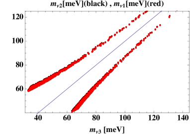
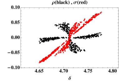
Figure 1: Allowed regions in the planes of $m_{\nu_{3}}$-$m_{\nu_{1,2}}$ meV (left) and $\delta$-$(\rho,\sigma)$ (right), where $\delta$ and $(\rho,\sigma)$ are the Dirac and Majorana CP phases, respectively.

The mass matrices for the lepton sector are given by

$$M_{\ell} =\left[\begin{array}[]{ccc}m_{e}&0&0\\ 0&m_{\mu}&0\\ 0&0&m_{\tau}\\ \end{array}\right],\quad M_{D}=\left[\begin{array}[]{ccc}m_{D_{1}}&0&0\\ 0&m_{D_{2}}&0\\ 0&0&m_{D_{3}}\\ \end{array}\right],\quad M_{N}=\left[\begin{array}[]{ccc}m_{N_{11}}&m_{N_{12}}&0\\ m_{N_{12}}&m_{N_{22}}&m_{N_{23}}\\ 0&m_{N_{23}}&0\\ \end{array}\right],$$ (37)

where $m_{e,\mu,\tau}\equiv y_{\ell_{1,2,3}}v_{0}/\sqrt{2}$, $m_{D_{1,2,3}}\equiv y_{\nu_{1,2,3}}v_{0}/\sqrt{2}$, $m_{N_{11}}\equiv y_{N_{1}}v^{\prime}_{0}/\sqrt{2}$, $m_{N_{22}}\equiv y_{N_{2}}v^{\prime}_{1}/\sqrt{2}$, $m_{N_{12}}\equiv y_{N_{12}}v^{\prime}_{2}/\sqrt{2}$, $m_{N_{23}}\equiv y_{N_{23}}v^{\prime}_{3}/\sqrt{2}$. After applying the seesaw mechanism, the active neutrino mass matrix $m_{\nu}$ is given by

$$m_{\nu}\approx-M_{D}^{T}M^{-1}_{N}M_{D}=\left[\begin{array}[]{ccc}\times&0&\times\\ 0&0&\times\\ \times&\times&\times\\ \end{array}\right],$$ (41)

where $m_{\nu}$ is defined by the diagonalized matrix of $D_{\nu}=U_{MNS}^{\dagger}m_{\nu}U^{*}_{MNS}$. Clearly, the active neutrino mass matrix is a successful two-zero texture that provides some predictions in fig. 1, and the formulas are simply found by directly solving the following two relations Fritzsch:2011qv :

$$(m_{\nu})_{12}=(U_{MNS}D_{\nu}U^{T}_{MNS})_{12}=0,\quad(m_{\nu})_{22}=(U_{MNS}D_{\nu}U^{T}_{MNS})_{22}=0,$$ (42)

where we have used the experimental values at 3$\sigma$ confidential level (C.L.) Forero:2014bxa . The left plane in fig. 1 represents the allowed region of $m_{\nu_{1}}$(red) and $m_{\nu_{2}}$(black) in terms of $m_{\nu_{3}}$, where the unit is meV. It suggests that this texture allows both of normal and inverted hierarchies, given by 65 meV$\lesssim m_{\nu_{3}}\lesssim$125 meV and 30 meV$\lesssim m_{\nu_{3}}\lesssim$115 meV, respectively. The right figure demonstrates the Majorana phases $(\rho,\sigma)$ in terms of the Dirac one $\delta$. It implies that the Dirac phase is predicted to be $4.65\lesssim\delta\lesssim 4.78$, $-0.05\lesssim\rho\lesssim 0.05$ and $-0.09\lesssim\sigma\lesssim 0.09$ at 3$\sigma$ C.L.. Therefore, $\delta\approx 3\pi/2$ is found to be the best fit value.

II.2 Muon related phenomenologies

We now focus on the interactions between fermions and new gauge bosons $(Z^{\prime}_{2},Z^{\prime}_{3})$. Since the masses of $Z^{\prime}_{2,3}$ are not seriously constrained by the LEP or LHC experiment, they do not couple to the electron/positron. The relevant interacting Lagrangian is given by

$${\cal L} \sim\frac{Z^{\prime\mu}_{2}}{3}\bar{d}_{L_{i}}\gamma_{\mu}d_{L_{j}}\left[g^{\prime}_{2}c_{\theta}(V^{\dagger}_{CKM})_{d_{i}c}(V_{CKM})_{cd_{j}}-g^{\prime}_{3}s_{\theta}(V^{\dagger}_{CKM})_{d_{i}t}(V_{CKM})_{td_{j}}\right]$$

$$+\frac{Z^{\prime\mu}_{3}}{3}\bar{d}_{L_{i}}\gamma_{\mu}d_{L_{j}}\left[g^{\prime}_{2}s_{\theta}(V^{\dagger}_{CKM})_{d_{i}c}(V_{CKM})_{cd_{j}}+g^{\prime}_{3}c_{\theta}(V^{\dagger}_{CKM})_{d_{i}t}(V_{CKM})_{td_{j}}\right]$$

$$-g^{\prime}_{2}\bar{\mu}\gamma_{\mu}\mu(c_{\theta}Z^{\prime\mu}_{2}+s_{\theta}Z^{\prime\mu}_{3})$$ (43)

$$\equiv\frac{Z^{\prime\mu}_{2}}{3}\bar{d}_{L_{i}}\gamma_{\mu}d_{L_{j}}{\cal O}_{2_{d_{i}d_{j}}}+\frac{Z^{\prime\mu}_{3}}{3}\bar{d}_{L_{i}}\gamma_{\mu}d_{L_{j}}{\cal O}_{3_{d_{i}d_{j}}}-g^{\prime}_{2}c_{\theta}Z^{\prime\mu}_{2}\bar{\mu}\gamma_{\mu}\mu-g^{\prime}_{2}s_{\theta}Z^{\prime\mu}_{3}\bar{\mu}\gamma_{\mu}\mu.$$ (44)

$B\to K^{*}\mu\bar{\mu}$: The effective Lagrangian to explain the $B\to K^{*}\mu\bar{\mu}$ anomaly is given by

$$i{\cal L}\approx i\frac{g^{\prime}_{2}}{3}\left(\frac{c_{\theta}{\cal O}_{2_{sb}}}{m_{Z^{\prime}_{2}}^{2}}+\frac{s_{\theta}{\cal O}_{3_{sb}}}{m_{Z^{\prime}_{3}}^{2}}\right)(\bar{s}\gamma^{\mu}P_{L}b)(\bar{\mu}\gamma_{\mu}\mu)\,,$$ (45)

which leads to the $\Delta C_{9}^{\mu}$ operator to be

$$\Delta C_{9}^{\mu}\approx\frac{\sqrt{2}\pi g^{\prime}_{2}}{\alpha_{em}G_{F}(V_{CKM})_{tb}(V^{*}_{CKM})_{ts}}\left(\frac{c_{\theta}{\cal O}_{2_{sb}}}{m_{Z^{\prime}_{2}}^{2}}+\frac{s_{\theta}{\cal O}_{3_{sb}}}{m_{Z^{\prime}_{3}}^{2}}\right).$$ (46)

The most recent global fit of $\Delta C_{9}^{\mu}$ can be found in Ref. Arbey:2019duh , given by

$${-\Delta C_{9}^{\mu}}=1.03\pm 0.20.$$ (47)

Remarkably, there are no additional constraints, such as those from $B_{s/d}\to\bar{\mu}\mu$ and ${\rm BR}(B\to K\mu^{+}\mu^{-})/{\rm BR}(B\to Ke^{+}e^{-})$, since the Lagrangian does not contain the $\Delta C_{10}$ operator and $Z^{\prime}_{2}$ does not directly interact with the electron/positron.

$M-\overline{M}$ meson mixings: The extra gauge boson induces the neutral meson mixings of $M-\bar{M}$ at the tree level, where $M=(K^{0},B_{d},B_{s})$. The formulas for the mass splittings are given by Gabbiani:1996hi

$$\Delta m_{K}^{0}\approx \frac{2}{3}\left(\frac{|{\cal O}_{2_{sd}}|^{2}}{m_{Z^{\prime}_{2}}^{2}}+\frac{|{\cal O}_{3_{sd}}|^{2}}{m_{Z^{\prime}_{3}}^{2}}\right)m_{K}f^{2}_{K},$$ (48)

$$\Delta m_{B_{d}}^{0}\approx \frac{2}{3}\left(\frac{|{\cal O}_{2_{bd}}|^{2}}{m_{Z^{\prime}_{2}}^{2}}+\frac{|{\cal O}_{3_{bd}}|^{2}}{m_{Z^{\prime}_{3}}^{2}}\right)m_{B_{d}}f^{2}_{B_{d}},$$ (49)

$$\Delta m_{B_{s}}^{0}\approx \frac{2}{3}\left(\frac{|{\cal O}_{2_{bs}}|^{2}}{m_{Z^{\prime}_{2}}^{2}}+\frac{|{\cal O}_{3_{bs}}|^{2}}{m_{Z^{\prime}_{3}}^{2}}\right)m_{B_{s}}f^{2}_{B_{s}},$$ (50)

which should be less than the experimental values of $(3.48\times 10^{-4},3.33\times 10^{-2},1.17)\times 10^{-11}$ GeV Olive:2016xmw , where $f_{M}=(156,191,200)$ MeV and $m_{M}=(0.498,5.280,5.367)$ GeV, respectively.

Bound from the LHC: The data from the LHC experiments Aaboud:2017buh also restrict the ratio between the extra gauge couplings and their masses. Here, we estimate them by applying the effective Lagrangian with the resulting relation, give by

$$\frac{(30\ {\rm TeV})^{2}}{12\pi}\lesssim\frac{1}{g^{\prime}_{2}}\left(\frac{c_{\theta}{\cal O}_{2_{dd}}}{m_{Z^{\prime}_{2}}^{2}}+\frac{s_{\theta}{\cal O}_{3_{dd}}}{m_{Z^{\prime}_{3}}^{2}}\right)^{-1}.$$ (51)

This constraint will be taken into consideration in the numerical analysis.

Before showing numerical analysis, we discuss the relations between $B\to K^{*}\mu\bar{\mu}$ and the mixings of $M-\bar{M}$, especially $\Delta B_{d,s}$, involving the bottom quark, which are strongly constrained by the experimental data. Consequently, one finds that $\Delta C_{9}\approx 0.1$ at most, which is smaller than the value in Eq. (47) by one order of magnitude. To enhance $\Delta C_{9}$, we can introduce one set of vector quarks: $Q^{\prime}\equiv[U^{\prime},D^{\prime}]^{T}$ and $d^{\prime}$, which are $SU(2)_{L}$ doublet and singlet, respectively, along with one complex boson inert $S$. The additional gauged charges assigned as (0,-1/3,0) and (0,2/3,0) for $(Q^{\prime},d^{\prime})$ and $S$, respectively. Then, we write the new part of the Lagrangian as

$$-{\cal L} =f_{2}\bar{Q}_{L_{2}}Q^{\prime}_{R}S+g_{2}\bar{d}_{R_{2}}d^{\prime}_{L}S+M^{\prime}\bar{Q}^{\prime}Q^{\prime}+m^{\prime}\bar{d}^{\prime}d^{\prime}+m_{S}^{2}|S|^{2}+{\rm h.c.}$$

$$\rightarrow F^{\dagger}_{i2}\bar{d}_{L_{i}}d^{\prime}_{R}S+G^{\dagger}_{i2}\bar{d}_{R_{i}}d^{\prime}_{L}S+M^{\prime}\bar{D}^{\prime}D^{\prime}+m^{\prime}\bar{d}^{\prime}d^{\prime}+m_{S}^{2}|S|^{2}+{\rm h.c.},$$ (52)

where $F^{\dagger}_{i2}(G^{\dagger}_{i2})\equiv V^{\dagger}_{CKM_{i2}}f_{2}(g_{2})$. Here, we have neglected the mass term $\bar{Q}^{\prime}d^{\prime}$ and additional Higgs potential related to $S$ as well as and the diagonal up-quark sector for simplicity. Subsequently, we find that the $M-\bar{M}$ mixings from the box diagrams are given by

$$\Delta m_{K}^{1}\approx \frac{m_{K}f_{K}^{2}}{3(4\pi)^{2}}\left[(F_{22}^{*}F_{21})^{2}F_{box}(m_{S},M^{\prime})+(G_{21}^{*}G_{22})^{2}F_{box}(m_{S},m^{\prime})\right],$$ (53)

$$\Delta m_{B_{d}}^{1}\approx \frac{m_{B_{d}}f^{2}_{B_{d}}}{3(4\pi)^{2}}\left[(F_{23}^{*}F_{21})^{2}F_{box}(m_{S},M^{\prime})+(G_{21}^{*}G_{23})^{2}F_{box}(m_{S},m^{\prime})\right],$$ (54)

$$\Delta m_{B_{s}}^{1}\approx \frac{m_{B_{s}}f^{2}_{B_{s}}}{3(4\pi)^{2}}\left[(F_{23}^{*}F_{22})^{2}F_{box}(m_{S},M^{\prime})+(G_{22}^{*}G_{23})^{2}F_{box}(m_{S},m^{\prime})\right],$$ (55)

$$F_{box}(m_{1},m_{2}) =\frac{m_{1}^{2}-m_{2}^{2}+m_{2}^{2}\ln\left(\frac{m_{2}^{2}}{m_{1}^{2}}\right)}{(m_{1}^{2}-m_{2}^{2})^{2}}.$$ (56)

When $F_{21,22}$ and $G_{21}$ are taking to be pure imaginary, $G_{23}\approx 0$, and the others are real, Eqs. (53)-(55) can be simplified as

$$\Delta m_{K}^{1}\approx \frac{m_{K}f_{K}^{2}}{3(4\pi)^{2}}\left[|F_{22}|^{2}|F_{21}|^{2}F_{box}(m_{S},M^{\prime})-|G_{21}|^{2}|G_{22}|^{2}F_{box}(m_{S},m^{\prime})\right],$$ (57)

$$\Delta m_{B_{d}}^{1}\approx -\frac{m_{B_{d}}f^{2}_{B_{d}}}{3(4\pi)^{2}}|F_{23}|^{2}|F_{21}|^{2}F_{box}(m_{S},M^{\prime}),$$ (58)

$$\Delta m_{B_{s}}^{1}\approx -\frac{m_{B_{s}}f^{2}_{B_{s}}}{3(4\pi)^{2}}|F_{23}|^{2}|F_{22}|^{2}F_{box}(m_{S},M^{\prime})\,,$$ (59)

respectively, leading to

$$\Delta m_{K}^{total} \approx\Delta m_{K}^{1}\approx\frac{m_{K}f_{K}^{2}}{3(4\pi)^{2}}\left[|F_{22}|^{2}|F_{21}|^{2}F_{box}(m_{S},M^{\prime})-|G_{21}|^{2}|G_{22}|^{2}F_{box}(m_{S},m^{\prime})\right],$$ (60)

$$\Delta m_{B_{d}}^{total} \approx\Delta m_{B_{d}}^{0}+\Delta m_{B_{d}}^{1}\approx\left[\frac{|{\cal O}_{2_{bd}}|^{2}}{m_{Z^{\prime}_{2}}^{2}}+\frac{|{\cal O}_{3_{bd}}|^{2}}{m_{Z^{\prime}_{3}}^{2}}-\frac{|F_{23}|^{2}|F_{21}|^{2}}{3(4\pi)^{2}}F_{box}(m_{S},M^{\prime})\right]m_{B_{d}}f^{2}_{B_{d}},$$ (61)

$$\Delta m_{B_{s}}^{total} \approx\Delta m_{B_{s}}^{0}+\Delta m_{B_{s}}^{1}\approx\left[\frac{|{\cal O}_{2_{bd}}|^{2}}{m_{Z^{\prime}_{2}}^{2}}+\frac{|{\cal O}_{3_{bd}}|^{2}}{m_{Z^{\prime}_{3}}^{2}}-\frac{|F_{23}|^{2}|F_{22}|^{2}}{3(4\pi)^{2}}F_{box}(m_{S},M^{\prime})\right]m_{B_{s}}f^{2}_{B_{s}},$$ (62)

where $\Delta m_{K}^{0}$ is negligibly small. Thus, we do not need to consider the constraints of the $M-\bar{M}$ mixings, since we can expect that the contributions get canceled among Eqs.(60)-(62).

III Numerical analysis

In our numerical analysis, we explore the allowed region of $-\Delta C_{9}$, by randomly selecting the input parameters of $g^{\prime}_{1,2,3}$ and $m_{Z^{\prime}_{2,3}}$, along with all the constraints discussed above. Then, each of the scan range is taken to be

$$v^{\prime}_{1,2,3}\in[10^{3},10^{7}]\ {\rm GeV},\quad g^{\prime}_{2,3}\in[10^{-5},\sqrt{4\pi}].$$ (63)

Fig. 2 shows the possible regions in the planes of $s_{\theta}$-$(-\Delta C_{9})$ (left) and $g^{\prime}_{2(3)}/m_{Z^{\prime}_{2,3}}$-$(-\Delta C_{9})$ (right), where the horizontal black (green) line corresponds to the observed value of 1.03 ($\pm$0.20), which is allowed by the experiment in Eq. (47). The figure at the left-handed side of Fig. 2 suggests that a larger $s_{\theta}$ is favored with the allowed lowest range being about $0.2$. The right-handed figure in Fig. 2 indicates that $g^{\prime}_{3}/m_{Z^{\prime}_{3}}$ does not depend on $-\Delta C_{9}$ so much, whereas $g^{\prime}_{2}/m_{Z^{\prime}_{2}}$ does, resulting in the allowed ranges of $g^{\prime}_{3}/m_{Z^{\prime}_{3}}\lesssim 0.10$ and $0.13\lesssim g^{\prime}_{2}/m_{Z^{\prime}_{2}}\lesssim 0.16$.

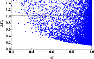
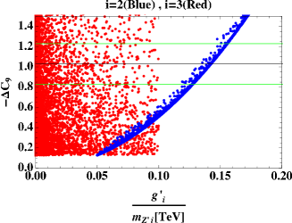
Figure 2: Allowed regions in the planes of $s_{\theta}$-$(-\Delta C_{9})$ (left) and $g^{\prime}_{2,3}/m_{Z^{\prime}_{2,3}}$-$(-\Delta C_{9})$ (right), where the horizontal black (green) line corresponds to the observed value of 1.03 ($\pm$0.20), allowed by the experiment in Eq. (47).

IV Conclusions and Discussions

We have proposed a model with flavor dependent gauged symmetries of $U(1)_{B_{1}-L_{1}}\times U(1)_{B_{2}-L_{2}}\times U(1)_{B_{3}-L_{3}}$. In this framework, we have formulated the renormalizable Yukawa Lagrangian, Higgs potential and kinetic term. We have found that no additional Higgs boson is needed to avoid the dangerous GB, which is one of the main modification of the model in Ref. Mu:2018weh . Based on the successful two-zero texture, we are able to give several predictions in the lepton sector as concretely shown in our numerical analysis. We have also formulated the mass matrix in the additional neutral gauge bosons, and successfully decomposed the electron/positron specific gauge boson and the others, imposing some assumptions. Due to this decomposition, the strong constraint from LEP experiment has been evaded. This is also an improvement on the model in Ref. Mu:2018weh . Finally, we have done a global numerical analysis by including all of the valid constraints, and illustrated the allowed region to satisfy the anomaly of $B\to K^{*}\bar{\mu}\mu$ via additional gauge bosons.

References

(1)
R. Aaij et al. [LHCb Collaboration],
Phys. Rev. Lett. 113 (2014) 151601.
(2)
R. Aaij et al. [LHCb Collaboration],
JHEP 1708, 055 (2017).
(3)
R. Aaij et al. [LHCb Collaboration],
JHEP 1509, 179 (2015).
(4)
V. Khachatryan et al. [CMS Collaboration],
Phys. Lett. B 753, 424 (2016).
(5)
J. P. Lees et al. [BaBar Collaboration],
Phys. Rev. D 93, 052015 (2016).
(6)
J.-T. Wei et al. [Belle Collaboration],
Phys. Rev. Lett. 103, 171801 (2009).
(7)
T. Aaltonen et al. [CDF Collaboration],
Phys. Rev. Lett. 108, 081807 (2012).
(8)
R. Aaij et al. [LHCb Collaboration],
JHEP 1602, 104 (2016).
(9)
S. Wehle et al. [Belle Collaboration],
Phys. Rev. Lett. 118, 111801 (2017).
(10)
A. M. Sirunyan et al. [CMS Collaboration],
Phys. Lett. B 781, 517 (2018).
(11)
J. P. Lees et al. [BaBar Collaboration],
Phys. Rev. D 88, 072012 (2013).
(12)
R. Aaij et al. [LHCb Collaboration],
Phys. Rev. Lett. 115, no. 11, 111803 (2015);
Erratum: [Phys. Rev. Lett. 115, 159901 (2015)].
(13)
T. Hurth, F. Mahmoudi and S. Neshatpour,
Nucl. Phys. B 909, 737 (2016).
(14)
G. D’Amico et al., JHEP 1709, 010 (2017).
(15)
W. Altmannshofer, P. Stangl, and D.M. Straub,
Phys. Rev. D 96, 055008 (2017).
(16)
G. Hiller and I. Nisandzic,
Phys. Rev. D 96, 035003 (2017).
(17)
L.S. Geng et al., Phys. Rev. D 96, 093006 (2017).
(18)
M. Ciuchini et al., Eur. Phys. J. C 77, 688 (2017).
(19)
A. Celis, J. Fuentes-Martin, A. Vicente, and J. Virto,
Phys. Rev. D 96, 035026 (2017).
(20)
T. Hurth et al., Phys. Rev. D 96, 095034 (2017).
(21)
B. Capdevila, A. Crivellin, S. Descotes-Genon, J. Matias, and J. Virto,
JHEP 1801, 093 (2018).
(22)
G. Hiller and F. Kruger,
Phys. Rev. D 69, 074020 (2004).
(23)
M. Bordone, G. Isidori and A. Pattori,
Eur. Phys. J. C 76, 440 (2016).
(24)
P. Ko, T. Nomura and H. Okada,
Phys. Lett. B 772, 547 (2017).
(25)
P. Ko, T. Nomura and H. Okada,
Phys. Rev. D 95, 111701 (2017).
(26)
M. Bordone, G. Isidori and S. Trifinopoulos,
Phys. Rev. D 96, 015038 (2017).
(27)
L. Bian, S. M. Choi, Y. J. Kang and H. M. Lee,
Phys. Rev. D 96, 075038 (2017).
(28)
C. Bonilla, T. Modak, R. Srivastava and J. W. F. Valle,
Phys. Rev. D 98, 095002 (2018).
(29)
Y. Tang and Y. L. Wu,
Chin. Phys. C 42, 033104 (2018).
(30)
L. Mu, H. Okada and C. Q. Geng,
Chin. Phys. C 42, 123106 (2018).
(31)
C. H. Chen and T. Nomura,
Phys. Lett. B 777, 420 (2018).
(32)
B. Allanach and J. Davighi,
arXiv:1809.01158 [hep-ph].
(33)
A. Kamada, M. Yamada and T. T. Yanagida,
arXiv:1811.02567 [hep-ph].
(34)
H. Fritzsch, Z. z. Xing and S. Zhou,
JHEP 1109, 083 (2011).
(35)
N. Cabibbo, Phys. Rev. Lett.10, 531 (1963); M.
Kobayashi and T. Maskawa, Prog. Theor. Phys.49, 652 (1973).
(36)
Z. Maki, M. Nakagawa and S. Sakata, Prog. Theor. Phys.28, 870 (1962);
B. Pontecorvo, Zh. Eksp. Teor. Fiz.53, 1717 (1967);
Sov. Phys. JETP26, 984(1968).
(37)
D. V. Forero, M. Tortola and J. W. F. Valle,
Phys. Rev. D 90, 093006 (2014).
(38)
A. Arbey, T. Hurth, F. Mahmoudi, D. Martinez Santos and S. Neshatpour,
arXiv:1904.08399 [hep-ph].
(39)
F. Gabbiani, E. Gabrielli, A. Masiero and L. Silvestrini,
Nucl. Phys. B 477, 321 (1996).
(40)
C. Patrignani et al. [Particle Data Group],
Chin. Phys. C 40, 100001 (2016).
(41)
M. Aaboud et al. [ATLAS Collaboration],
JHEP 1710, 182 (2017).
(42)
A. M. Sirunyan et al. [CMS Collaboration],
Phys. Lett. B 778, 263 (2018).
(43)
P. T. P. Hutauruk, T. Nomura, H. Okada and Y. Orikasa,
Phys. Rev. D 99, 055041 (2019).