The effect of the liquid layer thickness on the
dissolution of immersed surface droplets

Abstract

Droplets on a liquid-immersed solid surface are key elements in many applications, such as high-throughput chemical analysis and droplet-templated porous materials. Such surface droplets dissolve when the surrounding liquid is undersaturated and the dissolution process is usually treated analogous to a sessile droplet evaporating in air. Typically, theoretical models predict the mass loss rate of dissolving droplets as a function of droplet geometrical factors (radius, constant angle), and droplet material properties (diffusion constant and densities), where the thickness of the surrounding liquid layer is neglected. Here, we investigate, both numerically and theoretically, the effect of the liquid layer thickness on the dissolution of surface droplets. We perform $3D$ lattice Boltzmann simulations and obtain the density distribution and time evolution of droplet height during dissolution. Moreover, we find that the dissolution slows down and the lifetime linearly increases with increasing the liquid layer thickness. We propose a theoretical model based on a quasistatic diffusion equation which agrees quantitatively with simulation results for thick liquid layers. Our results offer insight to the fundamental understanding of dissolving surface droplets and can provide valuable guidelines for the design of devices where the droplet lifetime is of importance.

I Introduction

Droplets on a substrate immersed in a liquid film have practical implications for a wide range of applications from biomolecular analysis and chemical reactions in microfluidic devices to high-resolution imaging techniques ^{1; 2; 3; 4}. Such surface droplets can be produced by the solvent exchange method ^{5; 6}, microprinting ⁷, emulsion direct adsorption ⁸ and others ⁹.

If the surrounding liquid is undersaturated with droplet liquid, the droplets dissolve. The dissolution process of surface droplets is similar to the dissolution of surface bubbles ^{10; 11} and the evaporation of sessile droplets ¹². There are two physical mechanisms that can affect the dissolution rate of a surface droplet. The first mechanism is the rate at which liquid molecules cross the droplet interface. The second mechanism is the transport of the droplet liquid away from the droplet surface in the surrounding liquid. Normally, the transfer rate of liquid molecules across the interface is much faster than the diffusion rate of the liquid ¹². Thus, the dissolution rate of the droplet is dominated by the diffusion of droplet liquid into the surrounding environment. The diffusion of droplet liquid is driven by the gradient of the droplet liquid in the surrounding liquid, and the time-dependent density of droplet liquid in the surrounding liquid follows the unsteady diffusion equation, known as Fick’s second law

$$\partial\rho_{1}/\partial t=D\nabla^{2}\rho_{1},$$ (1)

where $D$ is the diffusion constant for droplet liquid in surrounding liquid and $\rho_{1}$ is the density of the droplet liquid. Here, we denote the droplet liquid as liquid $1$ and the surrounding liquid as liquid $2$. Due to dissolution, the volume of the drop decreases until it is fully dissolved. We assume that the convective transport of liquid $1$ induced by the density difference between liquid $1$ and liquid $2$ is negligible. The diffusion timescale is characterized by $t_{df}\sim R^{2}/D$, where $R$ is the base radius of the droplets, as shown in Fig. 1. The dissolution timescale can be expressed as $t_{ds}\sim\rho^{1}_{d}/(\rho^{1}_{s}-\rho^{1}_{top})t_{df}$, where $\rho^{1}_{d}$ is the density of liquid $1$ inside the droplet, $\rho^{1}_{s}$ is the saturation density of liquid $1$ near the droplet surface and $\rho^{1}_{top}$ is the density of liquid $1$ in the ambient air. The ratio between the dissolution timescale and diffusion timescale $t_{ds}/t_{df}\sim\rho^{1}_{d}/(\rho^{1}_{s}-\rho^{1}_{top})$ is typically much larger than $10^{2}$. Therefore, the time-dependent term in Eq. (1) can be neglected and the density of liquid $1$ follows a quasi-steady diffusion equation $D\nabla^{2}\rho_{1}=0$. For the dissolution of droplet arrays, as shown in Fig. 1, the boundary conditions are: i) the density of liquid $1$ equals the saturation density along the droplet surface, $\rho^{1}_{r_{k}=R}=\rho^{1}_{s}$, where $r_{k}$ is the local radial coordinate of droplet $k$ ; ii) the liquid density at the liquid-air interface is the liquid density in the ambient air, $\rho^{1}_{z=L_{z}}=\rho^{1}_{top}$; iii) the substrate is impermeable, $\partial\rho_{1}/\partial z=0$ along the substrate. There is no analytical solution available for the unsteady diffusion equation or even the quasistatic diffusion equation with the above boundary conditions.

Figure 1: Sketch of a regular array of surface droplets containing liquid $1$ sitting on a substrate and covered by a layer of another liquid (liquid $2$) of thickness $L_{z}$. The maximum height of the droplets is denoted by $h$ and the radius of their footprint is $R$. $L$ is the center to center distance between neighboring droplets.

In the case where the liquid layer thickness $L_{z}$ is much larger than the droplet height, $L_{z}/h\rightarrow\infty$, and the inter-distance of droplets is much larger than the droplet base radius, $L/R\rightarrow\infty$, the system can be treated like a single dissolving surface droplet, which is analogous to a sessile droplet evaporating in an open air environment. During evaporation of a droplet, the quasistatic diffusion equation for the concentration field $\rho$, $\nabla^{2}\rho=0$ is then used to predict the evaporation rate along the surface of the droplet ^{13; 14; 15}. The boundary conditions become: i) the density of liquid $1$ equals the saturation density along the droplet surface, $\rho=\rho_{s}$; ii) the liquid density far away from the droplet is $\rho_{\infty}$; iii) the substrate is impermeable, $\partial\rho/\partial z=0$ along the substrate. Assuming the effect of gravity can be neglected, the droplet takes a spherical cap shape dominated by surface tension. In this case, the evaporation flux $J=-D\nabla\rho$ is analogous to the electric potential distribution around a charged lens-shaped conductor and an analytical solution was derived by Lebedev ¹⁶. Popov ¹⁵ used this analytical solution and obtained the total mass flux by integrating the evaporation flux over the droplet surface,

$$\frac{dM}{dt}=-\pi RD(\rho_{s}-\rho_{\infty})$$

$$\left(\frac{\sin\theta}{1+\cos\theta}+4\int_{0}^{\infty}\frac{1+\cosh 2\theta\epsilon}{\sinh 2\theta\epsilon}\tanh\left[(\pi-\theta)\epsilon\right]d\epsilon\right)\mbox{,}$$ (2)

where $\theta$ is the contact angle of the droplet.

Dietrich et al. ^{7; 17} applied the quasistatic diffusion approach and Eq. (2) to study the dissolution of single and multiple $1$-heptanol or $3$-heptanol surface droplets in a container filled with undersaturated water. They find good agreement between experimental data and the above equation in the limit where the surrounding water is still highly undersaturated after all the droplets are dissolved ^{7; 18; 17}. However, different from evaporating droplets in an open air environment, the surrounding liquid film during dissolution of surface droplets can be saturated while the surface droplets are still present. Then, the dissolution rate of the droplets is determined by the diffusion rate of their liquid in the liquid environment and the distance the droplet liquid has to travel to reach the ambient air (see Fig. 1). In this case, the total mass flux is determined by integrating the diffusive flux along the free surface where the liquid meets the ambient air. Thus, the layer thickness of the surrounding liquid is expected to play an important role on the dissolution rate and the lifetime of dissolving surface droplets.

In the remainder of this paper, we numerically investigate the effect of the layer thickness on the dissolution and the lifetime of dissolving surface droplets. We carry out $3D$ lattice Boltzmann simulations with a diffusion dominated dissolution model. A substrate is located at the bottom of the system and a surface droplet is deposited on the substrate covered by another liquid layer of thickness $L_{z}$. Periodic boundary conditions are applied at the sides of the system, to mimic an infinite system with uniformly distributed droplets. We initially saturate the liquid layer and then apply the dissolution boundary condition at the top of the system. Different modes of contact line dynamics during dissolution such as constant angle (CA) and constant radius (CR) modes are studied. We find that the droplet lifetime is proportional to the layer thicknesses $L_{z}$. The simulations are accompanied by a theoretical analysis based on a quasistatic diffusion equation which confirms the simulation result.

II Simulation Method

Our simulations are based on the lattice Boltzmann method (LBM) which can be seen as an alternative way to approximate solutions of the Navier-Stokes equations ¹⁹ and which was demonstrated to be a powerful tool to simulate multiphase/multicomponent fluids ^{19; 20; 21}. We use the pdeudopotential multicomponent LBM proposed by Shan and Chen ²⁰, which has been successfully applied to a wide range of multiphase/multicomponent flow problems during the past two decades ²². A number of groups have simulated problems related to the diffusion or evaporation of fluids using the LBM recently. Ledesma-Aguilar et al. ^{23; 24} present a diffusion based evaporation method based on the free energy multiphase lattice Boltzmann method and demonstrate quantitative agreement with several benchmark cases as well as qualitative agreement with experiments involving evaporating droplet arrays. Jansen et al. ²⁵ study the evaporation of droplets on a chemically patterned substrate and qualitatively compare the simulation results with experimental data. Our group recently applied the LBM together with the multicomponent method of Shan and Chen successfully to study the evaporation of a planar film, a floating droplet, a sessile droplet, and a colloidal suspension droplet ^{26; 27}. In the following we review some details of the method and refer the reader to the relevant literature for a more detailed description and our implementation ^{28; 29; 30; 31; 32; 26; 21; 27}.

In our implementation, two fluid components $c=1,2$ follow the evolution of their individual distribution functions discretized in space and time,

$$f_{i}^{c}(\mathbf{x}+\mathbf{e}_{i}\Delta t,t+\Delta t)-f_{i}^{c}(\mathbf{x},t)=$$

$$-\frac{\Delta t}{\tau^{c}}\left[f_{i}^{c}(\mathbf{x},t)-f_{i}^{\mathrm{eq}}(\rho^{c}(\mathbf{x},t),\mathbf{u}^{c}(\mathbf{x},t))\right]\mbox{,}$$ (3)

where $i=1,...,19$. $f_{i}^{c}(\mathbf{x},t)$ are the single-particle distribution functions for each fluid component and $\mathbf{e}_{i}$ is the discrete velocity in the $i$th direction. $\tau^{c}$ is the relaxation time for component $c$. We define the macroscopic densities and velocities for each component as $\rho^{c}(\mathbf{x},t)=\rho_{0}\sum_{i}f^{c}_{i}(\mathbf{x},t)$, where $\rho_{0}$ is a reference density, and $\mathbf{u}^{c}(\mathbf{x},t)=\sum_{i}f^{c}_{i}(\mathbf{x},t)\mathbf{e}_{i}/\rho^{c}(\mathbf{x},t)$, respectively. Here, $f_{i}^{\mathrm{eq}}$ is a second-order equilibrium distribution function ³³, defined as

$$f_{i}^{\mathrm{eq}}(\rho^{c},\mathbf{u}^{c})=\omega_{i}\rho^{c}\bigg{[}1+\frac{\mathbf{e}_{i}\cdot\mathbf{u}^{c}}{c_{s}^{2}}-\frac{\left(\mathbf{u}^{c}\cdot\mathbf{u}^{c}\right)}{2c_{s}^{2}}+\frac{\left(\mathbf{e}_{i}\cdot\mathbf{u}^{c}\right)^{2}}{2c_{s}^{4}}\bigg{]}\mbox{.}$$ (4)

$\omega_{i}$ is a coefficient depending on the direction: $\omega_{0}=1/3$ for the zero velocity, $\omega_{1,\dots,6}=1/18$ for the six nearest neighbors and $\omega_{7,\dots,18}=1/36$ for the nearest neighbors in diagonal direction. $c_{s}=\frac{1}{\sqrt{3}}\frac{\Delta x}{\Delta t}$ is the speed of sound. When sufficient lattice symmetry is guaranteed, the Navier-Stokes equations can be recovered from Eq. (II) on appropriate length and time scales ¹⁹. For convenience we choose the lattice constant $\Delta x$, the timestep $\Delta t$, the unit mass $\rho_{0}$ and the relaxation time $\tau^{c}$ to be unity in the remainder of this article, which leads to a kinematic viscosity $\nu^{c}$ $=$ $\frac{1}{6}$ in lattice units. We note that the conversion from lattice units to physical units can be performed e.g. by matching dimensionless numbers, such as the Reynolds number or the Schmidt number ³⁴.

Following the work of Shan and Chen ²⁰, we apply a mean-field interaction force

$$\mathbf{F}^{c}(\mathbf{x},t)=-\Psi^{c}(\mathbf{x},t)\sum_{\bar{c}}\sum_{i}\omega_{i}g_{c\bar{c}}\Psi^{\bar{c}}(\mathbf{x}+\mathbf{e}_{i},t)\mathbf{e}_{i}$$ (5)

between fluid components $c$ and $\bar{c}$, in which $g_{c\bar{c}}$ is a constant interaction parameter. Here, $\Psi^{c}(\mathbf{x},t)$ is chosen as the functional form $\Psi^{c}(\mathbf{x},t)\equiv\Psi(\rho^{c}(\mathbf{x},t))=1-e^{-\rho^{c}(\mathbf{x},t)}$. We apply this force $\mathbf{F}^{c}(\mathbf{x},t)$ to the component $c$ by adding a shift $\Delta\mathbf{u}^{c}(\mathbf{x},t)=\frac{\tau^{c}\mathbf{F}^{c}(\mathbf{x},t)}{\rho^{c}(\mathbf{x},t)}$ to the velocity $\mathbf{u}^{c}(\mathbf{x},t)$ in the equilibrium distribution.

Inspired by the work of Huang et al., an interaction force is introduced between the fluid and the substrate ³⁵,

$$\mathbf{F}^{c}(\mathbf{x})=-g_{wc}\Psi^{c}(\mathbf{x})\sum_{i}\omega_{i}s(\mathbf{x}+\mathbf{e}_{i})\mathbf{e}_{i}\mbox{,}$$ (6)

where $g_{wc}$ is a constant. Here, $s(\mathbf{x}+\mathbf{e}_{i})=1$ if $\mathbf{x}+\mathbf{e}_{i}$ is a solid lattice site, and $s(\mathbf{x}+\mathbf{e}_{i})=0$ otherwise. An approximate formula can be used to estimate the contact angle $\theta$ of a droplet on the substrate ³⁵:

$$\cos(\theta)=\frac{g^{wc}-g^{w\bar{c}}}{g^{c\bar{c}}[\Psi(\rho^{c})-\Psi(\rho^{\bar{c}})]/2}$$ (7)

The phase separation can be triggered by choosing a proper interaction parameter $g_{c\bar{c}}$ in Eq. (5). Each component separates into a denser majority phase of density $\rho_{ma}$ and a lighter minority phase of density $\rho_{mi}$, respectively ²⁰. To simulate dissolution, we impose the distribution function of component $c$ at the boundary sites $\mathbf{x}_{H}$ as ²⁶

$$f_{i}^{c}(\mathbf{x}_{H},t)=f_{i}^{\mathrm{eq}}\left(\rho_{H}^{c},\mathbf{u}^{c}_{H}(\mathbf{x}_{H},t)\right),$$ (8)

in which $\mathbf{u}^{c}_{H}(\mathbf{x}_{H},t)=0$. Furthermore, for simplicity, we ensure total mass conservation within the system by setting the density of component $\bar{c}$ as

$$\rho^{\bar{c}}(\mathbf{x}_{H},t)=\rho^{c}(\mathbf{x}_{H},t-1)+\rho^{\bar{c}}(\mathbf{x}_{H},t-1)-\rho^{c}_{H},$$ (9)

so that the distribution functions of component $\bar{c}$ at the dissolution boundary sites $\mathbf{x}_{H}$ become

$$f_{i}^{\bar{c}}(\mathbf{x}_{H},t)=f_{i}^{\mathrm{eq}}\left(\rho_{H}^{\bar{c}},\mathbf{u}^{\bar{c}}_{H}(\mathbf{x}_{H},t)\right),$$ (10)

where $\mathbf{u}^{\bar{c}}_{H}(\mathbf{x}_{H},t)=0$. When the imposed density $\rho_{H}^{c}$ is lower than the equilibrium minority density $\rho_{mi}^{c}$, a density gradient develops in the lighter minority phase of component $c$. This gradient drives component $c$ to diffuse towards the dissolution boundary, which recovers the unsteady diffusion equation Eq. (1) validated in our previous work ²⁶. In the case that the densities of two components are similar, the bouyancy-driven convective flow can be neglected, and the dissolution is diffusion dominated and the diffusivity is given by ²⁶

$$D^{c}=\biggl{[}c_{s}^{2}(\tau-\frac{1}{2})-\frac{c_{s}^{2}}{\rho^{c}+\rho^{\bar{c}}}(\rho^{\bar{c}}\Psi^{c}g_{c\bar{c}}\Psi^{{}^{\prime}\bar{c}}+\rho^{c}\Psi^{\bar{c}}g_{\bar{c}c}\Psi^{{}^{\prime}c})\biggr{]},$$ (11)

where $\Psi^{{}^{\prime}c}$ and $\Psi^{{}^{\prime}\bar{c}}$ are the spatial derivative of $\Psi^{c}$ and $\Psi^{\bar{c}}$, respectively. A similar approach was recently introduced by Ledesma-Aguilar et al. for a free energy lattice Boltzmann method ²³.

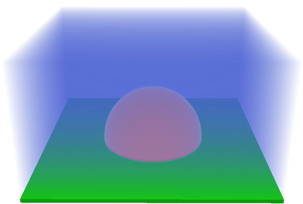
Figure 2: Snapshot of a surface droplet (red) sitting on a liquid (blue) immersed substrate (green) obtained from our simulations. The system size is $256\times 256\times 144$. We apply the dissolution boundary at the top plane and periodic boundary conditions at the sides of the system.

III Results and discussion

(a) $t/T=0.0$

(b) $t/T=0.28$

(c) $t/T=0.57$

(d) $t/T=0.85$

Figure 3: Time evolution of the density distribution of liquid $1$ during droplet dissolution obtained from our simulation. The color represents the density and the white solid lines are iso-density lines. The droplet dissolves in constant radius mode. The position of the top surface corresponds to the top of the pictures.

We simulate an infinite array of immersed droplets on a substrate as depicted in Fig. 1. A snapshot from a simulation of a 3D unit cell is shown in Fig. 2. The system size is $L\times L\times L_{z}$, where $L=256$ and $L_{z}$ is chosen to be $L_{z}=72$, $144$, $288$, $576$, respectively. We initialize the system with a droplet containing liquid $1$ of density $\rho^{1}_{ma}=0.7$ and liquid $2$ of density $\rho^{2}_{mi}=0.04$. The surrounding volume consists of liquid $2$ of density $\rho^{2}_{ma}=0.7$ and liquid $1$ of density $\rho^{1}_{mi}=0.04$. The droplet has an initial radius $R_{0}=60$ and an initial contact angle $\theta_{0}=90^{\circ}$ corresponding to an initial maximum height $h_{0}=60$. The interaction strength in Eq. (5) is chosen to be $g_{12}=3.6$ leading to a diffusivity $D\approx 0.12$. The diffusion constant of the surrounding liquid in the droplet liquid is of similar order as the diffusion constant of the droplet liquid in the surrounding liquid. Furthermore, periodic boundary conditions are applied at the sides of the system to mimic an infinite array of identical droplets. After equilibration, we impose the dissolution boundary condition at the top of the system to mimic the ambient air. Our dissolution boundary condition allow to set a constant density and a zero velocity at the top boundary ²⁶. The droplet liquid diffuses from the droplet to the dissolution boundary, gradually forming a density gradient. We note that we only apply dissolution boundary conditions at the top surface. Therefore, due to mass conservation the total diffusive flux integrated along the droplet surface is consistent with the corresponding total flux at the top surface. The measurement of the lifetime of the droplet is only started once the gradient is fully developed. We investigate the effect of layer thickness $L_{z}$ by varying only the system size in $z$ direction and keeping all other parameters constant.

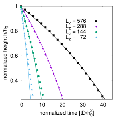
Figure 4: Time evolution of the droplet height during dissolution in CR mode. The symbols are simulation data for different system heights length $Lz=74$ (triangles), $144$ (circles), $288$ (diamonds), and $576$ (squares), respectively. The solid lines denote the theoretical prediction Eq. (19).

We start out our investigation with a dissolving droplet featuring a pinned contact line, the so-called constant radius (CR) mode. The substrate is chemically patterned with variable wettability: a superhydrophilic circle ($\theta\approx 0^{\circ}$) of radius $R_{s}=60$ is located at the center surrounded by a superhydrophobic area ($\theta\approx 180^{\circ}$).

Fig. 3 shows the time evolution of the density distribution of liquid $1$ during the dissolution for a system of size $256\times 256\times 288$. Near the top of the system, the density is homogeneous along the horizontal direction, while it follows the shape of the droplet in the vicinity of its surface. The density gradient is larger near the droplet surface than at a position far away from it. The dissolution flux is represented by the distance between the neighboring iso-density lines. In the early state (Fig. 3(a) and Fig. 3(b)), the dissolution flux near the contact line is smaller than that near the top of the droplet. This is due to the collective effect introduced by neighboring droplets ¹⁷ and in our case is an effect of the periodic boundary conditions in the horizontal directions. We note that this collective effect would become weaker when the droplet inter-distance increases, as observed in experiments ^{36; 17} In the later stage (Fig. 3(c) and Fig. 3(d)) when the contact angle is much smaller than $90^{\circ}$, the dissolution flux diverges towards the contact line, which is consistent with the theoretical prediction of Popov ¹⁵. In addition, the density gradient at the top of the system stays almost constant during the dissolution. This indicates that the effect of the curved droplet surface on the density distribution in the far field is negligible if the thickness of liquid layer $L_{z}$ is much larger than the droplet height $h_{0}$, $L_{z}\gg h_{0}$.

In Fig. 4 we show the simulation data (symbols) of the droplet height versus time for different system heights $Lz=74$ (triangles), $144$ (circles), $288$ (diamonds), and $576$ (squares), respectively. We note that the multicomponent model of Shan and Chen suffers from spurious vaporisation effects once the diameter of the droplets becomes $\approx 5-10$ lattice units. To avoid the effect of the spurious vaporisation on the analysis and to ensure a sufficient resolution, we only use simulation data for droplet heights larger than $20$. We note that the upper limit of droplet size is only given by the available computational resources. The method is furthermore valid as long as the droplets follow the continuum Navier Stokes assumptions and for sizes large enough so that thermal fluctuations do not play a role anymore. During the dissolution, the droplet height keeps decreasing, but with a slower rate when the length $L_{z}$ is increased. This is reasonable because liquid $1$ requires more time to diffuse through a thicker liquid layer to arrive at the top free surface. Moreover, the decreasing rate of the droplet height speeds up towards the end of the lifetime of the droplet.

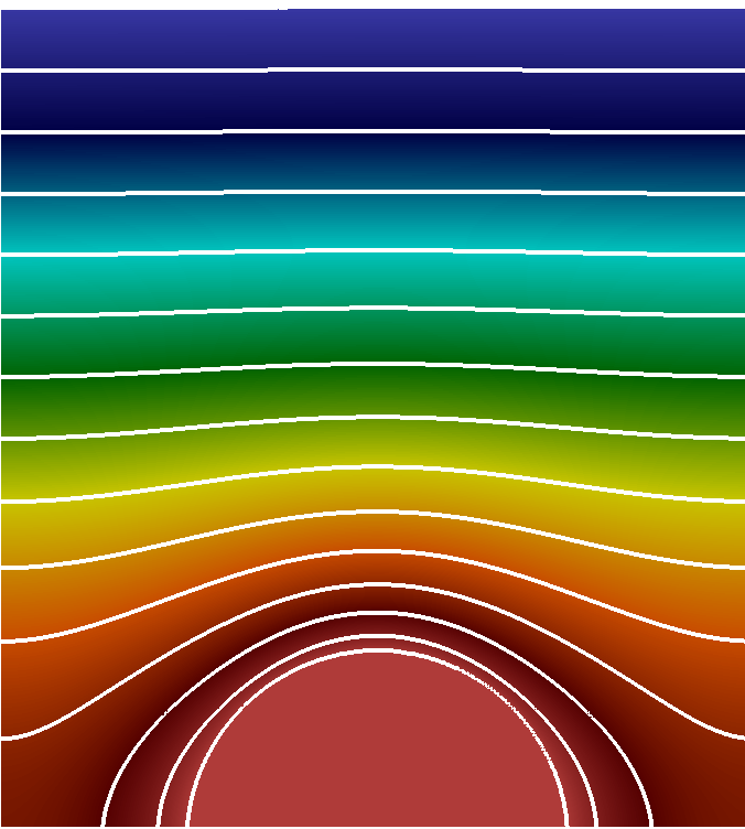
(a) $t/T=0.0$

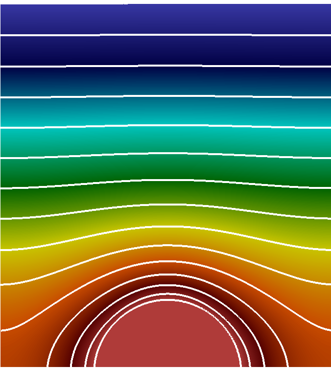
(b) $t/T=0.31$

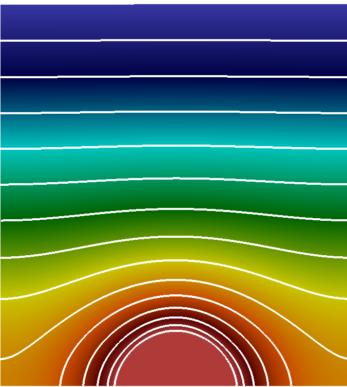
(c) $t/T=0.62$

(d) $t/T=0.93$

Figure 5: Time evolution of the density distribution of liquid $1$ during droplet dissolution obtained in our simulations. The color represents the density and the white solid lines are iso-density lines. The droplet dissolves in CA mode. The position of the top surface corresponds to the top of the pictures.

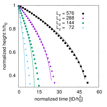
Figure 6: Time evolution of the droplet height during dissolution in CA mode. The symbols are simulation data for different system heights $Lz=74$ (triangles), $144$ (circles), $288$ (diamonds) and $576$ (squares), respectively. The solid lines follow the theoretical prediction given by Eq. (23).

Next, we investigate the dissolution of a droplet in constant angle (CA) mode. The substrate has a uniform wettability and the droplet keeps its contact angle of $90^{\circ}$ during the dissolution. We note that in some cases, if the surrounding liquid diffuses into the droplet, the surrounding droplet molecules may change the chemical potential, which affects the motion of the droplet and as such the contact angle variation ³⁷. However, in our system, the droplet is assumed to be saturated with the surrounding liquid and thus the diffusion of surrounding liquid into the droplet is prohibited. In Fig. 5 we show the variation of the density distribution of liquid $1$ during dissolution for a system size of $256\times 256\times 288$. Equivalent to the CR mode, the density distributes uniformly along the horizontal direction in the far field, whereas it is strongly affected by the curved droplet surface in the near field of the droplet. The density gradient increases when approaching the droplet surface. Again, the collective effect introduced by neighboring droplets on the density gradient is observed in the earlier stages (Fig. 5(a) and Fig. 5(b)). This collective effect become weaker when the droplet radius deceases (Fig. 5(c)) (i.e., the inter-spacing between neighboring droplets increases), which is consistent with experimental results ^{17; 36}. In the very late stage (Fig. 5(d)), the density gradient and thus the dissolution flux is uniform along the droplet surface, which is in agreement with the theoretical prediction of the evaporation flux along the surface of a droplet with $90^{\circ}$ contact angle ¹⁵.

In Fig. 6 we show the time evolution of droplet height obtained in our simulations (symbols) for different lengths $Lz=74$ (triangles), $144$ (circles), $288$ (diamonds) and $576$ (squares), respectively. Similar to the CR mode, the droplet height decreases more slowly with increasing length $L_{z}$. Additionally, the droplet shrinks faster towards the end of its lifetime. We note that the convective flow induced by the movement of the droplet interface during dissolution may have an effect on the effective dissolution rate ³⁸. To quantify the ratio of the contributions to mass transport by convection to those by diffusion, we calculate the Péclet number $Pe=lu/D$, where $l$ is a characteristic length, $u$ is a characteristic velocity and $D$ is the diffusion constant. Here, we have $u\sim 10^{-5}$, $D\sim 0.12$ and $l\sim 60$ in lattice Boltzmann units, and obtain $Pe\sim 10^{-3}$. The Péclet number is much smaller than $1$, therefore, the effect of convection near the droplet surface on the mass transfer is negligible. As discussed in the work of Zhao et al. ³⁸, the interfacial shape can be affected by the surface tension, viscosity and inertia during dissolution. In our system, the Reynolds number $Re=lu/\nu^{c}$ is of the order of $10^{-3}$ and thus we expect the effect of fluid inertia also to be negligible, i.e. the droplet adheres to a spherical cap shape.

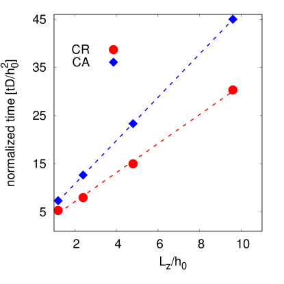
Figure 7: The normalized lifetime $tD/h_{0}^{2}$ of the dissolving surface droplet for systems with different height $L_{z}/h_{0}$. The symbols are simulation data for the CR mode (circles) and CA the mode (diamonds). The dashed lines are fitted linear functions, indicating that the lifetime is to a good approximation proportional to the layer thickness $L_{z}$.

In Fig. 7, we compare the lifetime $T$ of the dissolving surface droplet with increasing the layer thickness $L_{z}$ for both CR (circles) and CA (diamonds) modes. The dashed lines represent fitted linear functions. We reiterate that the time zero in our measured lifetime corresponds to a moment after the density gradient is fully developed in the system and the droplet maximal height just begins to decrease. The results demonstrate that the lifetime of the dissolving surface droplet is strongly dependent on the thickness of the liquid layer $L_{z}$, i.e. it increases approximately linearly with increasing height $L_{z}$ for both CR and CA mode.

In the following we propose a theoretical model for taking into account the effect of the layer thickness of the surrounding liquid on the lifetime of a dissolving surface droplet. We consider surface droplets of liquid $1$ sitting on a substrate covered by liquid $2$ of thickness $L_{z}$, as illustrated in Fig. 1. The droplets are uniformly distributed on the substrate with center to center distance $L$ and are of identical size with initial maximum height $h_{0}$, and initial radius of the contact line $R_{0}$. We assume that the droplet is surface tension dominated and thus adheres the shape of a spherical cap.

Assuming a diffusion dominated dissolution and the buoyancy-driven convection being negligible, the density of liquid $1$ follows a quasi-static diffusion equation

$$\partial_{t}\rho_{1}=D\nabla^{2}\rho_{1}=0.$$ (12)

In the case of $L_{z}\gg h$, we can assume that the density of the droplet liquid along the horizontal direction far away from the droplet surface is homogeneous. Furthermore, we can assume that the density varies linearly along the $z$ direction so that we can write the dissolution flux approximately as

$$J_{z}=\frac{-D(\rho^{1}_{s}-\rho^{1}_{top})}{L_{z}},$$ (13)

in which $\rho^{1}_{s}$ is the saturation density of liquid $1$ near the droplet surface and $\rho^{1}_{top}$ is the density of liquid $1$ in the ambient air.

With Eq. (13), we obtain the rate of mass of a single droplet released into the ambient air at the top surface as

$$dM/dt=L^{2}J_{z}=\frac{-DL^{2}(\rho^{1}_{s}-\rho^{1}_{top})}{L_{z}},$$ (14)

where $L^{2}$ represents the effective area of the top surface for the corresponding single droplet. Eq. (14) indicates that the rate of mass loss decreases with increasing layer thickness $L_{z}$, which is consistent with the simulation results indicating that the droplet height has a slower decreasing rate with increasing $L_{z}$ (see Fig. 4 and Fig. 6). Moreover, based on Eq. (14), when the layer thickness is fixed, the rate of mass loss can be treated as constant during the dissolution process. Thus, the height of the droplet decreases faster when the droplet volume decreases, which agrees qualitatively with the simulation results shown in Fig. 4 and Fig. 6, i.e. the decreasing rate of the droplet height increases towards the end of the life of the dissolving droplet. We note that Eq. 14 is equivalent to the Noyes-Whitney equation ^{39; 38}, which is generally used to describe the rate of a solute dissolving in a solvent.

By integrating Eq. (14), we get the time evolution of the droplet mass as

$$M=M_{0}-\frac{DL^{2}(\rho^{1}_{s}-\rho^{1}_{top})t}{L_{z}},$$ (15)

where $M_{0}$ is the initial mass of the droplet. From Eq. (15), we can obtain the lifetime of the droplet as

$$T=\frac{M_{0}L_{z}}{DL^{2}(\rho^{1}_{s}-\rho^{1}_{top})}.$$ (16)

Eq. (16) shows that the dissolution time is proportional to the length $L_{z}$, which is consistent with our simulation results shown in Fig. 7.

The total mass of a spherical cap-shaped droplet is

$$M=\frac{\pi\rho^{1}_{d}h}{6}(3R^{2}+h^{2}),$$ (17)

where $\rho^{1}_{d}$ is the density of liquid $1$ inside the droplet. In the case of the droplet being dissolved in CA mode ($R=R_{0}$), we obtain the time derivative of the total mass from Eq. (17) as

$$dM/dt=\frac{\pi\rho^{1}_{d}}{2}(R_{0}^{2}+h^{2})dh/dt.$$ (18)

By comparing Eq. (18) and Eq. (14), we reach

$$dh/dt=\frac{-2DL^{2}(\rho^{1}_{s}-\rho^{1}_{top})}{\pi\rho^{1}_{d}L_{z}}\frac{1}{R_{0}^{2}+h^{2}}.$$ (19)

Eq. 19 is solved numerically using a 4th-order Runge-Kutta algorithm and compared to the simulation results in Fig. 4 for different layer thicknesses $L_{z}=72$, $144$, $288$, $576$. Our theoretical model (solid lines) captures the qualitative features of the time evolution of the droplet height for all simulated systems and quantitatively agrees with the numerical results for a thick liquid layer, i.e. $L_{z}\geq 288$ ($L_{z}/h_{0}\geq 4$). We note that the increasing layer thickness induces a higher hydrostatic pressure, which may affect the stability of the surface droplets. In experiments, stable surface droplets are formed ^{5; 7} when the ratio of layer thickness and droplet height is of order $10^{3}$. This range is similar to our simulation parameters. A detailed understanding of the effect of the hydrostatic pressure on the stability of the droplet calls for a systematic experimental investigation and extensive theoretical analysis, which is beyond the scope of the current work.

If the droplet dissolves in the CA mode ($\theta=\theta_{a}$), we can write its total mass as

$$M=\frac{\pi\rho^{1}_{d}(3\sin\theta_{a}+\cos\theta_{a}-1)}{3(1-\cos\theta_{a})}h^{3}$$ (20)

and then we obtain the time derivative of mass as

$$dM/dt=\frac{\pi\rho^{1}_{d}(3\sin\theta_{a}+\cos\theta_{a}-1)h^{2}}{(1-\cos\theta_{a})}dh/dt.$$ (21)

By comparing Eq. (21) with Eq. (14), we get

$$dh/dt=\frac{-DL^{2}(\rho^{1}_{s}-\rho^{1}_{top})}{L_{z}\rho^{1}_{d}\pi}\frac{1-\cos\theta_{a}}{3\sin\theta_{a}+\cos\theta_{a}-1}\frac{1}{h^{2}}.$$ (22)

If the contact angle of the droplet is $\theta_{a}=90^{\circ}$, Eq. (22) is simplified to

$$dh/dt=\frac{-DL^{2}(\rho^{1}_{s}-\rho^{1}_{top})}{2L_{z}\rho^{1}_{d}\pi}\frac{1}{h^{2}}.$$ (23)

In Fig. 6 we again compare the theoretical analysis Eq. (23) with simulation results for different layer thicknesses $L_{z}=72$, $144$, $288$, $576$. As in the previous case, our theoretical model agrees qualitatively with the simulation results for all the systems and we obtain quantitative agreement with simulation results for very thick liquid layers, i.e. $L_{z}=576$ ($L_{z}/h_{0}\geq 9$).

The good agreement between the theoretical model and our simulation results for both CR and CA modes indicates that the limiting diffusion process is at the top interface and the dynamics of the contact line of the droplet can be neglected for predicting the lifetime of dissolving surface droplet if $L_{z}\gg h_{0}$. The theoretical model performs worse when the droplet dissolves in CA instead of in CR mode. A possible explanation is that our model is valid in the limit of densely distributed droplets on the substrate $L/2R_{0}\approx 1$ and it does not consider the variation of the distance between neighboring droplets. In CR mode, the distance of neighboring droplets keeps constant, whereas it increases in CA mode. This increase weakens the collective effect and induces a sharp non-linear decrease of the density around the droplet surface (Fig. 5(d)). The latter is less accurately described by the dissolution flux equation (Eq. (13)) assuming a linear density gradient. We note that our lattice Boltzmann simulations recover the unsteady diffusion equation. Therefore, the good agreement between our simulation results and our theoretical model also indicates that the quasistatic diffusion assumption is valid for $L_{z}\gg h_{0}$.

IV Conclusion

We demonstrated that the thickness of the liquid layer surrounding immersed and dissolving surface droplets strongly influences the dissolution and the lifetime of the droplets. This holds if the density gradient of the droplet liquid is fully developed in the surrounding liquid. We performed $3D$ lattice Boltzmann simulations of the dissolution of droplets in both constant radius and constant angle modes. In the near field of the droplet, we observed the convective effect introduced by neighboring droplets on the density gradient and the divergence of the dissolution flux near the contact line for small contact angles, which is consistent with experimental observations ¹⁷ and theoretical contributions ¹⁵. However, in the far field of the droplet, the density is homogeneous along the horizontal direction and its gradient stays almost constant during dissolution when the liquid layer thickness is much larger than the droplet height. Additionally, in both modes, the lifetime of the dissolving droplets increases approximately linearly with increasing the thickness of the liquid layer.

We proposed a simple theoretical model assuming a quasistatic diffusion equation in the limit of liquid layer thickness much larger than the droplet height $L_{z}/h\gg 1$. Our model predicts that the rate of mass loss is a linear function of layer thickness $L_{z}$, which confirms the simulation results. Moreover, our model qualitatively captures the time evolution of the droplet height and agrees quantitatively with simulation results for thick liquid layers. Surprisingly, even in the range where the layer thickness is similar to the droplet height, $L_{z}\approx h$, the lifetime predicted by our theoretical model is of the same order as the one obtained from the simulations. Therefore, our model can be used to estimate the lifetime of dissolving droplets quickly regardless of the thickness of the liquid layer and the modes of contact line dynamics.

In a future work we plan to extend this study to non-regularly distributed surface droplets and droplets with polydisperse sizes ^{5; 6}. It would be also interesting to investigate the effect of liquid layer thickness on the buoyancy-driven convective flow ¹⁸ when the two liquids have a large density difference. Our lattice Boltzmann method can be directly applied to this problem because it recovers the Navier-Stokes and unsteady diffusion equations ²⁶.