Simple Semi-Grant-Free Transmission Strategies Assisted by Non-Orthogonal Multiple Access

Abstract

Grant-free transmission is an important feature to be supported by future wireless networks since it reduces the signalling overhead caused by conventional grant-based schemes. However, for grant-free transmission, the number of users admitted to the same channel is not caped, which can lead to a failure of multi-user detection. This paper proposes non-orthogonal multiple-access (NOMA) assisted semi-grant-free (SGF) transmission, which is a compromise between grant-free and grant-based schemes. In particular, instead of reserving channels either for grant-based users or grant-free users, we focus on an SGF communication scenario, where users are admitted to the same channel via a combination of grant-based and grant-free protocols. As a result, a channel reserved by a grant-based user can be shared by grant-free users, which improves both connectivity and spectral efficiency. Two NOMA assisted SGF contention control mechanisms are developed to ensure that, with a small amount of signalling overhead, the number of admitted grant-free users is carefully controlled and the interference from the grant-free users to the grant-based users is effectively suppressed. Analytical results are provided to demonstrate that the two proposed SGF mechanisms employing different successive interference cancelation decoding orders are applicable to different practical network scenarios.

I Introduction

Non-orthogonal multiple access (NOMA) has been recently recognized as a promising solution to realize the three key performance requirements of next-generation mobile networks, namely enhanced Mobile Broadband (eMBB), Ultra Reliable Low Latency Communications (URLLC), and massive Machine Type Communications (mMTC) [1, 2, 3]. For example, existing studies have demonstrated that the use of NOMA can significantly improve the system throughput for downlink and uplink transmission without consuming extra bandwidth, which is particularly important for eMBB [4, 5, 6]. Since NOMA ensures that multiple users can be served in the same time/frequency resource, the users do not have to wait for serving even if there are not sufficient orthogonal resource blocks available, and hence the latency experienced by the users is reduced, which is a useful feature for the support of URLLC [7, 8, 9]. The key challenge in realizing mMTC is the support of massive connectivity, given the scarce bandwidth resources, for which NOMA is a perfect solution as it encourages users to share their bandwidth resources instead of solely occupying them [10, 11, 12]. While the application of NOMA to eMBB has been extensively studied, there are few works on the application of NOMA to URLLC and mMTC.

This paper focuses on the application of NOMA to grant-free transmission which is an important feature to be included in mMTC and URLLC. The basic idea of grant-free transmission is that a user is encouraged to transmit whenever it has data to send, without getting a grant from the base station. Therefore, the lengthy handshaking process between the user and the base station is avoided and the associated signalling overhead is reduced. The key challenge for grant-free transmission is contention, as multiple users may choose the same channel to transmit at the same time. To resolve this problem, two types of grant-free solutions have been proposed. One is to exploit spatial degrees of freedom by applying massive multiple-input multiple-output (MIMO) to resolve contention [13, 14]. The other is to apply the NOMA principle and use sophisticated multi-user detection (MUD) methods, such as parallel interference cancellation (PIC) and compressed sensing [15, 16, 17]. In general, these grant-free schemes can be viewed as special cases of random access, where the base station does not play any role in multiple access, similar to computer networks. As a result, there is no centralized control for the number of users participating in contention, which means that these grant-free protocols fail if there is an excessive number of active users/devices, a likely situation for mMTC and URLLC.

The aim of this paper is to design NOMA assisted semi-grant-free (SGF) transmission schemes, which can be viewed as a compromise between grant-free transmission and conventional grant-based schemes. In particular, instead of reserving channels either for grant-based users or grant-free users, we focus on an SGF communication scenario in this paper, where one user is admitted to a channel via a conventional grant-based protocol and the other users are admitted to the same channel in an opportunistic and grant-free manner. User connectivity can be improved by considering this scenario with a combination of grant-based and grant free protocols, as all channels in the network are opened up for grant-free transmission, even if they have been reserved by grant-based users. In order to guarantee that the quality of service (QoS) requirements of the grant-based users are met, the contention among the opportunistic grant-free users needs to be carefully controlled to ensure that the grant-free users transmit only if they do not cause too much performance degradation to the grant-based users. Note that such contention control is not possible with pure grant-free protocols [13, 14, 15, 16, 17].

Two SGF schemes for contention control are proposed in this paper, where, unlike pure grant-free transmission, multiple access is still controlled by the base station, but with lower signalling overhead compared to the grant-based case. For the first proposed SGF scheme, the base station controls multiple access by broadcasting a threshold value to all users and also provides a criterion for the users to determine if they are qualified for transmission, a strategy similar to random beamforming [18, 19]. As a result, the contention control is realized in an open-loop manner, which does not require the users’ channel state information (CSI) to be known at the base station prior to transmission. Compared to grant-based transmission, less signalling overhead is introduced by SGF since all users which satisfy the criterion set by the base station are allowed to transmit immediately, without going through individual handshaking processes. Compared to grant-free transmission, in SGF, the number of the users admitted to the same channel can be carefully controlled, which helps avoid MUD failure due to an excessive number of admitted users. For the second proposed SGF scheme, distributed contention control is applied, where a fixed number of users with favourable channel conditions is granted access. We note that, for the proposed open-loop SGF scheme, the number of users admitted to the same channel is random, similar to conventional grant-free transmission. In other words, open-loop SGF may still admit more users to the same channel than can be supported, whereas the proposed SGF scheme with distributed contention control ensures that a fixed number of users is granted access.

The design of the proposed SGF protocols largely depends on the decoding order of successive interference cancellation (SIC) at the base station. For example, if the grant-based user’s signal is decoded in the first stage of SIC, in order to reduce the performance degradation experienced by this user, the opportunistic users which are additionally granted access to the same channel should have weak channel conditions. On the other hand, if the grant-based user’s signal is decoded in the last stage of SIC, strong grant-free users should be granted the right to transmit. The impact of the SIC decoding order on the performance of the proposed SGF protocols is investigated. Particularly, for open-loop SGF, the threshold broadcasted by the base station and the criterion for the users to determine if they are qualified for transmission are designed based on the adopted SIC decoding order, whereas for SGF with distributed contention control, the criterion for user contention is adapted to the SIC decoding order. Analytical results are provided to demonstrate the superior performance of the proposed NOMA assisted SGF protocols and also the impact of different SIC decoding orders on suitable application scenarios for the proposed SGF protocols. In particular, if the grant-based user’s signal is decoded in the first stage of SIC, the proposed SGF protocols are suited for the scenario, where the grant-based user is close to the base station and the grant-free users are cell-edge users. On the other hand, if the grant-based user’s signal is decoded in the last stage of SIC, the proposed SGF protocols are ideally suited for the scenario, where the grant-based user is a cell-edge user and the grant-free users are close to the base station.

II System Model

Consider an SGF uplink NOMA scenario, where multiple users are admitted to the same channel via a combination of grant-based and grant-free protocols. In particular, among these users, assume that there is one user, denoted by $\textrm{U}_{0}$, which needs to be served with high priority. Via a grant-based protocol, $\textrm{U}_{0}$ is allocated a dedicated orthogonal resource block, denoted by $\text{B}_{0}$, for its uplink transmission. In addition, there are $M$ grant-free users, denoted by $\textrm{U}_{m}$, $1\leq m\leq M$, which do not have time-critical data and compete with each other for admission to $\text{B}_{0}$ in an opportunistic manner. In a typical machine-type communication network, $\textrm{U}_{0}$ may be a sensor for healthcare monitoring or critical care, and $\textrm{U}_{m}$, $1\leq m\leq M$, may be sensors for power meters or environmental monitoring. In this SGF scenario, all channels in the network are available for grant-free transmission, even if they have been reserved by grant-based users. Hence, massive connectivity can be supported in a spectrally efficient manner.

II-A Assumptions for SGF Protocol Design

The proposed SGF protocols are designed under the following assumptions:

• Recall that $\textrm{U}_{0}$ is admitted to $\text{B}_{0}$ by using a grant-based protocol. It is assumed that via the broadcast signalling during the handshaking process between $\text{U}_{0}$ and the base station, $\textrm{U}_{0}$’s CSI as well as its transmit power, denoted by $P_{0}$, become available at the base station and at all grant-free users in an error-free manner.

• Prior to multiple access, each user knows its own CSI perfectly, but the base station does not acquire the CSI of the grant-free users, $\textrm{U}_{m}$, $1\leq m\leq M$, which reduces the signalling overhead. Via the proposed SGF protocols, a portion of the $M$ users are granted access. We assume that there is a sufficient number of orthogonal preambles for the base station to acquire the CSI of the transmitting grant-free users in order to facilitate MUD.

• $\textrm{U}_{m}$, $1\leq m\leq M$, are admitted to $\text{B}_{0}$ under the condition that the target data rate of $\text{U}_{0}$, denoted by $R_{0}$, can still be achieved with high probability, such that the QoS requirements of $\text{U}_{0}$ are satisified.

• We assume that all users’ channels, denoted by $h_{m}$, $0\leq m\leq M$, exhibit independent and identically distributed (i.i.d.) quasi-static Rayleigh fading. The ordered channel gains are denoted by $h_{(m)}$, where $|h_{(1)}|^{2}\leq\cdots\leq|h_{(M)}|^{2}$.

II-B Low-Overhead Protocols for Contention Control

A key step for SGF transmission is low-overhead contention control. In this paper, we focus on two types of low-overhead protocols, as described in the following:

II-B1 Open-loop contention control

The base station broadcasts a channel quality threshold $\tau$. The users decide whether to join the NOMA transmission by comparing their channel gains to $\tau$. A user is admitted if its channel gain is below or above the threshold depending on the SIC order employed by the base station, see Sections III and IV.

II-B2 Distributed contention control

Distributed contention control has been extensively studied in the contexts of opportunistic carrier sensing [20] and timer-backoff-based sensor selection [21, 22]. Take the distributed contention control mechanism proposed in [20] as an example, which selects the user with the strongest (or the weakest) channel for channel access. Once the contention time window starts, each user chooses a backoff $\tau_{m}$, which is a strictly decreasing (or increasing) function of the user’s channel gain. A user transmits a beacon to the base station after $\tau_{m}$ expires, provided that $\tau_{m}$ is smaller than the contention time window. As such, the user with the best (or worst) channel condition waits for the shortest time and hence identifies itself to the base station first. This method will be adopted for distributed contention control for the proposed SGF schemes. We note that more advanced distributed contention control schemes can select multiple strong (or weak) users, and a user can acquire the other users’ CSI by using the time differences between the transmitted beacons [20].

The design of the proposed SGF schemes depends on the SIC decoding order, as illustrated in the following two sections.

III Semi-Grant-Free Protocol - Type I

In this section, we assume that the message from $\text{U}_{0}$ is decoded in the first stage of SIC at the base station.

III-A Open-Loop Contention Control

The base station broadcasts a threshold $\tau$, which can be interpreted analogous to metrics for the interference temperature in cognitive radio networks [23]. Unlike grant-free protocols, which grant all $M$ users access, here only users whose channel gains are below this threshold are admitted to $\text{B}_{0}$. Without loss of generality, assume that there are $N$ users whose channel gains can satisfy this condition and share $\text{B}_{0}$ with $\text{U}_{0}$.

In order to simplify notations, the noise power is assumed to be normalized, and hence the transmit signal-to-noise ratio (SNR) for $\mathrm{U}_{0}$’s signal is identical to the user’s transmit power, $P_{0}$. Furthermore, assume that all grant-free users $\mathrm{U}_{m}$ use the same transmit power, denoted by $\bar{P}$. Therefore, with SIC, the base station can support the following data rates for the $(N+1)$ users:

$$\left\{\log\left(1+\frac{|h_{0}|^{2}P_{0}}{\sum^{N}_{j=1}|h_{(j)}|^{2}\bar{P}+1}\right),\log\left(1+\frac{|h_{(i)}|^{2}\bar{P}}{\sum^{i-1}_{j=1}|h_{(j)}|^{2}\bar{P}+1}\right),1\leq i\leq N\right\}.$$ (1)

The impact of SGF NOMA transmission on the rates of $\text{U}_{0}$ and the $N$ grant-free users is studied separately in the following subsections.

III-A1 Impact of SGF transmission on $\text{U}_{0}$

Based on (1), the outage probability of $\text{U}_{0}$ is given by

$$\mathbb{P}_{0}^{\mathrm{I,OL}}= \sum_{n=1}^{M}\mathbb{P}(N=n)\underset{Q_{1}}{\underbrace{\mathbb{P}\left(\left.\log\left(1+\frac{|h_{0}|^{2}P_{0}}{\sum^{n}_{j=1}|h_{(j)}|^{2}\bar{P}+1}\right)<R_{0}\right|N=n\right)}}$$ (2)

$$+\mathbb{P}\left(|h_{(1)}|^{2}>\tau\right)\mathbb{P}\left(\left.\log\left(1+|h_{0}|^{2}P_{0}\right)<R_{0}\right|N=0\right),$$

where $\mathbb{P}(N=n)$ denotes the probability that there are $n$ grant-free users whose channel gains are smaller than $\tau$. The following theorem provides a closed-form expression for $\mathbb{P}_{0}^{\mathrm{I,OL}}$.

Theorem 1.

The outage probability of $\text{U}_{0}$ achieved by the proposed open-loop Type I SGF protocol can be expressed as follows:

$$\mathbb{P}_{0}^{\mathrm{I,OL}}= \sum_{n=1}^{M}\frac{M!}{n!(M-n)!}e^{-(M-n)\tau}\left(1-e^{-\tau}\right)^{n}\sum^{n}_{p=0}\frac{{n\choose p}(-1)^{p}e^{-p\tau}}{(1-e^{-\tau})^{n}}\left(\sum_{l=0}^{n-1}\frac{\epsilon_{0}P_{0}^{-1}\bar{P}e^{-\epsilon_{0}P_{0}^{-1}(1+\bar{P}p\tau)}}{(1+\epsilon_{0}P_{0}^{-1}\bar{P})^{(l+1)}}\right.$$

$$\left.+e^{-\epsilon_{0}P_{0}^{-1}}-e^{-\epsilon_{0}P_{0}^{-1}(1+\bar{P}p\tau)}\right)+\left(1-e^{-\epsilon_{0}P_{0}^{-1}}\right),$$ (3)

where $\epsilon_{0}=2^{R_{0}}-1$.

Proof.

See Appendix A. ∎

III-A2 Asymptotic analysis of $\mathbb{P}_{0}^{\mathrm{I,OL}}$

In order to obtain some intuition about $\mathbb{P}_{0}^{\mathrm{I,OL}}$, an asymptotic analysis is carried out in the following.

We first consider the case, where $\bar{P}$ is fixed, $P_{0}\rightarrow\infty$ and $\tau\sim\frac{1}{P_{0}}$. In this case, $\mathbb{P}_{0}^{\mathrm{I,OL}}$ can be approximated as follows:

$$\mathbb{P}_{0}^{\mathrm{I,OL}}\overset{(a)}{\approx} \epsilon_{0}P_{0}^{-1}\bar{P}\sum_{n=1}^{M}\frac{M!}{(n-1)!(M-n)!}e^{-(M-n)\tau}\sum^{n}_{p=0}{n\choose p}(-1)^{p}e^{-p\tau}+\epsilon_{0}P_{0}^{-1}$$ (4)

$$= \epsilon_{0}P_{0}^{-1}\bar{P}\sum_{n=1}^{M}\frac{M!}{(n-1)!(M-n)!}e^{-(M-n)\tau}\left(1-e^{-\tau}\right)^{n}+\epsilon_{0}P_{0}^{-1},$$

where step (a) follows by using the binomial expansion and the series expansion of the exponential function. The approximation of $\mathbb{P}_{0}^{\mathrm{I,OL}}$ can be further simplified as follows:

$$\mathbb{P}_{0}^{\mathrm{I,OL}}\approx \epsilon_{0}P_{0}^{-1}+\epsilon_{0}P_{0}^{-1}\bar{P}\sum_{n=1}^{M}\frac{M!}{(n-1)!(M-n)!\tau^{n}}e^{-(M-n)\tau}$$

$$\approx \epsilon_{0}P_{0}^{-1}+\underset{\Delta_{\mathbb{P}_{0}^{\mathrm{I,OL}}}}{\underbrace{\tau\epsilon_{0}P_{0}^{-1}\bar{P}Me^{-(M-1)\tau}}}.$$ (5)

Remark 1: Recall that the outage probability of $\text{U}_{0}$ is degraded by admitting the grant-free users to $\text{B}_{0}$. The approximation in (5) clearly shows this degradation, as $\Delta_{\mathbb{P}_{0}^{\mathrm{I,OL}}}$ is the extra cost for admitting the grant-free users to $\text{B}_{0}$. However, this cost goes to zero, if $\bar{P}$ is fixed, $P_{0}\rightarrow\infty$, and $\tau\sim\frac{1}{P_{0}}$. In other words, by carefully choosing $\tau$, $\bar{P}$, and $P_{0}$, it is possible to ensure that $\text{U}_{0}$ experiences the same outage probability with the proposed SGF scheme as in the grant-based case. However, SGF can ensure that more users are connected, compared to a grant-based scheme.

Remark 2: The importance of considering the case with large $P_{0}$ and small $\bar{P}$ is explained in the following. Recall that $P_{0}$ and $\bar{P}$ denote the transmit SNRs at $\text{U}_{0}$ and the grant-free users, respectively. Therefore, in practice, the case with large $P_{0}$ and small $\bar{P}$ represents an important uplink scenario, where the grant-based user is close to the base station and the grant-free users are at the edge of the cell. The proposed Type I SGF protocol is ideally suited to this scenario to support massive connectivity in this situation without causing significant performance degradation to the grant-based user.

Next, we consider a different case, where $\tau$ and $\bar{P}$ are fixed, and ${P}_{0}\rightarrow\infty$. In this case, $\mathbb{P}_{0}^{\mathrm{I,OL}}$ in (3) can be approximated as follows:

$$\mathbb{P}_{0}^{\mathrm{I,OL}}\approx \epsilon_{0}P_{0}^{-1}\bar{P}\sum_{n=1}^{M}\frac{M!}{n!(M-n)!}e^{-(M-n)\tau}\sum^{n}_{p=0}{n\choose p}(-1)^{p}e^{-p\tau}\left(n+p\tau\right)+\epsilon_{0}P_{0}^{-1}.$$ (6)

The sum of the binomial coefficients in the above equation can be simplified as follows:

$$\sum^{n}_{p=0}{n\choose p}(-1)^{p}e^{-p\tau}p=-ne^{-\tau}\left(1-e^{-\tau}\right)^{n-1}.$$ (7)

Therefore, the approximation of $\mathbb{P}_{0}^{\mathrm{I,OL}}$ can be simplified as follows:

$$\mathbb{P}_{0}^{\mathrm{I,OL}}\approx\epsilon_{0}P_{0}^{-1}+\underset{\Delta_{\mathbb{P}_{0}^{\mathrm{I,OL}}}}{\underbrace{\epsilon_{0}P_{0}^{-1}\bar{P}\sum_{n=1}^{M}\frac{M!e^{-(M-n)\tau}\left(1-e^{-\tau}\right)^{n-1}\left(1-e^{-\tau}-\tau e^{-\tau}\right)}{(n-1)!(M-n)!}}}.$$ (8)

Remark 3: Similar to the case considered in Remark 1, one can also observe that in this case the gap between the outage probabilities of the grant-based and SGF schemes, $\Delta_{\mathbb{P}_{0}^{\mathrm{I,OL}}}$, is reduced to zero as $P_{0}$ grows. The outage probability with a constant $\tau$ is worse than that with $\tau\sim\frac{1}{P_{0}}$. On the other hand, SGF with a constant $\tau$ can support more grant-free users than SGF with $\tau\sim\frac{1}{P_{0}}$, when $P_{0}\rightarrow\infty$. Following steps similar to the ones to obtain (5) and (8), one can show that $\mathbb{P}_{0}^{\mathrm{I,OL}}$ also approaches zero when $\tau$ and ${P}_{0}$ are fixed but $\bar{P}\rightarrow 0$.

III-A3 Impact of SGF transmission on grant-free users

Without loss of generality, assume that $N$ grant-free users have been selected by the proposed protocol. As shown in (1), the proposed Type I SGF protocol can support the following rates for the grant-free users:

$$\log\left(1+\frac{|h_{(i)}|^{2}\bar{P}}{\sum^{i-1}_{j=1}|h_{(j)}|^{2}\bar{P}+1}\right),$$ (9)

where $1\leq i\leq N$. Without loss of generality, assume that each grant-free user wants to send $L$ bits to the base station. The probability that the number of bits sent by grant-free user $i$ within $\text{B}_{0}$ is less than $L$ is given by

$$\mathbb{P}_{i}^{\mathrm{I,OL}}=\mathbb{P}\left(\mathrm{B}_{0}\log\left(1+\frac{|h_{(i)}|^{2}\bar{P}}{\sum^{i-1}_{j=1}|h_{(j)}|^{2}\bar{P}+1}\right)<L\right).$$ (10)

Remark 4: It is assumed that a user can adapt its transmit data rate according to (9), which requires that one user has access to the other users’ CSI. This CSI knowledge can be obtained by adopting the beacon-based distributed contention control scheme in [20], which can be applied in the open-loop mechanism not for contention control, but for one user to acquire other users’ CSI. However, if this CSI knowledge is not available to the users, the probability $\mathbb{P}_{i}^{\mathrm{I,OL}}$ in (10) can also be viewed as a lower bound on the outage probability, if each user uses $\breve{R}_{i}\triangleq\frac{L}{\mathrm{B}_{0}}$ as its target data rate.

The probability $\mathbb{P}_{i}^{\mathrm{I,OL}}$ can be calculated as follows:

$$\mathbb{P}_{i}^{\mathrm{I,OL}}= \mathbb{P}\left(\sum^{i-1}_{j=1}|h_{(j)}|^{2}>\breve{\epsilon}_{i}^{-1}|h_{(i)}|^{2}-\bar{P}^{-1}\right)$$ (11)

$$= \mathbb{P}\left(\sum^{i-1}_{j=1}|h_{(j)}|^{2}>\breve{\epsilon}_{i}^{-1}|h_{(i)}|^{2}-\bar{P}^{-1},|h_{(i)}|^{2}>\breve{\epsilon}_{i}\bar{P}^{-1}\right)+\mathbb{P}\left(|h_{(i)}|^{2}<\breve{\epsilon}_{i}\bar{P}^{-1}\right),$$

where $\breve{\epsilon}_{i}=2^{\breve{R}_{i}}-1$. Note that there is a hidden constraint $|h_{(i)}|^{2}<\tau$ since the channel gains of all selected users are smaller than $\tau$. It is important to point out that $|h_{(i)}|^{2}$ and $\sum^{i-1}_{j=1}|h_{(j)}|^{2}$ are correlated. To evaluate the probability $\mathbb{P}_{i}^{\mathrm{I,OL}}$, we note that, conditioned on $|h_{(i)}|^{2}$, $\sum^{i-1}_{j=1}|h_{(j)}|^{2}$ can be viewed as the sum of $(i-1)$ i.i.d. variables, denoted by $\breve{h}_{k}$, with the following cumulative distribution function (CDF):

$$F_{|\breve{h}_{k}|^{2}}(y)=\left\{\begin{array}[]{ll}\frac{1-e^{-y}}{1-e^{-|h_{(i)}|^{2}}},&\text{if}\quad y\leq|h_{(i)}|^{2}\\ 1,&\text{if}\quad y>|h_{(i)}|^{2}\end{array}\right..$$ (14)

Following steps similar to those in the proof for Theorem 1, conditioned on $|h_{(i)}|^{2}$, the probability density function (pdf) of $\sum^{i-1}_{j=1}|h_{(j)}|^{2}$ can be obtained as follows:

$$f_{\sum^{i-1}_{j=1}|h_{(j)}|^{2}}(y)=\sum^{i-1}_{p=0}\frac{{i-1\choose p}(-1)^{p}e^{-p|h_{(i)}|^{2}}}{(1-e^{-|h_{(i)}|^{2}})^{i-1}(i-2)!}(y-p|h_{(i)}|^{2})^{i-2}e^{-(y-p|h_{(i)}|^{2})}u(y-p|h_{(i)}|^{2}),$$ (15)

where $u(\cdot)$ denotes the unit step function. On the other hand, $|h_{(i)}|^{2}$ is the $i$-th smallest value among $N$ i.i.d. random variables following the distribution in (53), instead of (14). By applying order statistics [24], the pdf of $|h_{(i)}|^{2}$ can be found as follows:

$$f_{|h_{(i)}|^{2}}(x)= c_{N,i}\frac{e^{-x}(1-e^{-x})^{i-1}\left(e^{-x}-e^{-\tau}\right)^{N-i}}{(1-e^{-\tau})^{N}},$$ (16)

where $c_{N,i}=\frac{N!}{(i-1)!(N-i)!}$.

If $\tau\leq\breve{\epsilon}_{i}\bar{P}^{-1}$, the probability is given by

$$\mathbb{P}_{i}^{\mathrm{I,OL}}= \int^{\tau}_{0}f_{|h_{(i)}|^{2}}(x)dx=1,$$ (17)

otherwise,

$$\mathbb{P}_{i}^{\mathrm{I,OL}}= \int^{\breve{\epsilon}_{i}\bar{P}^{-1}}_{0}f_{|h_{(i)}|^{2}}(x)dx+\int_{\breve{\epsilon}_{i}\bar{P}^{-1}}^{\tau}f_{|h_{(i)}|^{2}}(x)\int^{\infty}_{\breve{\epsilon}_{i}^{-1}x-\bar{P}^{-1}}f_{\sum^{i-1}_{j=1}|h_{(j)}|^{2}}(y)dydx.$$ (18)

It is worth pointing out that the upper limit of the integration of the pdf of $\sum^{i-1}_{j=1}|h_{(j)}|^{2}$ should be $|h_{(i)}|^{2}(i-1)$, but it can be replaced by $\infty$ as shown in Lemma 2 in Appendix A.

Remark 5: The probability $\mathbb{P}_{i}^{\mathrm{I,OL}}$ can be evaluated numerically by substituting (15) and (16) into (18), but a closed-form expression is difficult to obtain due to the step function in (15).

III-B Distributed Contention Control

After the base station broadcasts $\tau$, assume that there are $N$ users whose channels are worse than $\tau$. Only these $N$ users are allowed to participate in contention and a fixed number of users will be admitted to $\text{B}_{0}$ by applying distributed contention control as discussed at the end of Section II. Due to space limitations, we will focus on the case that only one user is granted access, i.e., the user with channel gain $h_{(1)}$ is scheduled if $|h_{(1)}|^{2}<\tau$. Therefore, the outage probability of $\text{U}_{0}$ can be expressed as follows:

$$\mathbb{P}_{0}^{\mathrm{I,DCC}}= \sum_{n=1}^{M}\mathbb{P}\left(|h_{(n)}|^{2}<\tau,|h_{(n+1)}|^{2}>\tau\right)\mathbb{P}\left(\left.\log\left(1+\frac{|h_{0}|^{2}P_{0}}{|h_{(1)}|^{2}\bar{P}+1}\right)<R_{0}\right|N=n\right)$$ (19)

$$+\mathbb{P}\left(|h_{(1)}|^{2}>\tau\right)\mathbb{P}\left(\left.\log\left(1+|h_{0}|^{2}P_{0}\right)<R_{0}\right|N=0\right).$$

The outage probability in (19) can be equivalently expressed as follows:

$$\mathbb{P}_{0}^{\mathrm{I,DCC}}= \underset{Q_{2}}{\underbrace{\mathbb{P}\left((|h_{(1)}|^{2}<\tau,\log\left(1+\frac{|h_{0}|^{2}P_{0}}{|h_{(1)}|^{2}\bar{P}+1}\right)<R_{0}\right)}}$$ (20)

$$+\mathbb{P}\left(|h_{(1)}|^{2}>\tau,\log\left(1+|h_{0}|^{2}P_{0}\right)<R_{0}\right).$$

With some algebraic manipulations, $Q_{2}$ can be expressed as follows:

$$Q_{2}= \left(1-e^{-M\tau}\right)\left(1-e^{-\epsilon_{0}P_{0}^{-1}}\right)-e^{-M\tau}\left(e^{-\epsilon_{0}P^{-1}_{0}}-e^{-\epsilon_{0}P_{0}^{-1}(1+\bar{P}\tau)}\right)$$ (21)

$$+e^{M\bar{P}^{-1}}\frac{e^{-(1+M\bar{P}^{-1}\epsilon_{0}^{-1}P_{0})\epsilon_{0}P^{-1}_{0}}-e^{-(1+M\bar{P}^{-1}\epsilon_{0}^{-1}P_{0})\epsilon_{0}P_{0}^{-1}(1+\bar{P}\tau)}}{1+M\bar{P}^{-1}\epsilon_{0}^{-1}P_{0}}.$$

By substituting (21) into (20) and using the fact that the second probability in (20) is a product of two simple probabilities, $\mathbb{P}\left(|h_{(1)}|^{2}>\tau\right)=e^{-M\tau}$ and $\mathbb{P}\left(\log\left(1+|h_{0}|^{2}P_{0}\right)<R_{0}\right)=1-e^{-\epsilon_{0}P_{0}^{-1}}$, a closed-form expression for the outage probability of $\text{U}_{0}$ can be obtained for the case with distributed contention control.

In order to obtain some insight, consider the case, where $\bar{P}$ and $\tau$ are fixed, $P_{0}\rightarrow\infty$. In this case, we have

$$Q_{2}\approx \left(1-e^{-M\tau}\right)\epsilon_{0}P_{0}^{-1}-e^{-M\tau}\epsilon_{0}P_{0}^{-1}\bar{P}\tau$$ (22)

$$+e^{M\bar{P}^{-1}}\frac{e^{-(\epsilon_{0}P_{0}^{-1}+M\bar{P}^{-1})}-e^{-(\epsilon_{0}P_{0}^{-1}+M\bar{P}^{-1})(1+\bar{P}\tau)}}{1+M\bar{P}^{-1}\epsilon_{0}^{-1}P_{0}}.$$

$Q_{2}$ can be further approximated as follows:

$$Q_{2}\approx \left(1-e^{-M\tau}\right)\epsilon_{0}P_{0}^{-1}-e^{-M\tau}\epsilon_{0}P_{0}^{-1}\bar{P}\tau+\frac{1-\epsilon_{0}P_{0}^{-1}-e^{-M\tau}\left(1-\epsilon_{0}P_{0}^{-1}-\epsilon_{0}P_{0}^{-1}\bar{P}\tau\right)}{1+M\bar{P}^{-1}\epsilon_{0}^{-1}P_{0}}.$$ (23)

Therefore, the outage probability $\mathbb{P}_{0}^{\mathrm{I,DCC}}$ can be approximated as follows:

$$\mathbb{P}_{0}^{\mathrm{I,DCC}}\approx e^{-M\tau}\epsilon_{0}P_{0}^{-1}+\left(1-e^{-M\tau}\right)\epsilon_{0}P_{0}^{-1}-e^{-M\tau}\epsilon_{0}P_{0}^{-1}\bar{P}\tau$$

$$+\frac{1-\epsilon_{0}P_{0}^{-1}-e^{-M\tau}\left(1-\epsilon_{0}P_{0}^{-1}-\epsilon_{0}P_{0}^{-1}\bar{P}\tau\right)}{1+M\bar{P}^{-1}\epsilon_{0}^{-1}P_{0}}$$

$$= \epsilon_{0}P_{0}^{-1}-e^{-M\tau}\epsilon_{0}P_{0}^{-1}\bar{P}\tau+\frac{1-\epsilon_{0}P_{0}^{-1}-e^{-M\tau}\left(1-\epsilon_{0}P_{0}^{-1}-\epsilon_{0}P_{0}^{-1}\bar{P}\tau\right)}{1+M\bar{P}^{-1}\epsilon_{0}^{-1}P_{0}}.$$ (24)

With some algebraic manipulations, we can obtain the following lemma.

$\mathbf{Lemma}$ 1.

Consider the case, where $\bar{P}$ and $\tau$ are fixed, and $P_{0}\rightarrow\infty$. In this case, $\mathbb{P}_{0}^{\mathrm{I,DCC}}$ can be approximated as follows:

$$\mathbb{P}_{0}^{\mathrm{I,DCC}}\approx \epsilon_{0}P_{0}^{-1}+\underset{\Delta_{\mathbb{P}_{0}^{\mathrm{I,DCC}}}}{\underbrace{\epsilon_{0}P_{0}^{-1}\bar{P}\left(\frac{\left(1-e^{-M\tau}\right)}{M}-e^{-M\tau}\tau\right)}}.$$ (25)

Remark 6: From the asymptotic result in (25), one can observe that the difference between the outage probabilities for the cases where the grant-free user is and is not admitted to $\text{B}_{0}$, $\Delta_{\mathbb{P}_{0}^{\mathrm{I,DCC}}}$, approaches zero as $M$ approaches infinity. This is different from the previous case considered in (8), where increasing $M$ deteriorates the outage probability of $\text{U}_{0}$. In other words, the use of distributed contention control can effectively ensure that the performance of $\text{U}_{0}$ is guaranteed even if there are many grant-free users. We note, however, that the use of distributed contention control results in a higher system overhead than the open-loop scheme.

To analyze the performance of the selected grant-free user, assume that the number of users whose channel gains are below the threshold is fixed and denoted by $N$, $N>0$, i.e., the number of users which are qualified to participate in contention is assumed to be fixed, and the unordered channel gains of these users follow the distribution in (53). Therefore, the outage probability of the selected grant-free user is given by

$$\mathbb{P}_{1}^{\mathrm{I,DCC}}= 1-\mathbb{P}\left(\log\left(1+\frac{|h_{0}|^{2}P_{0}}{|h_{(1)}|^{2}\bar{P}+1}\right)>R_{0},\log\left(1+|h_{(1)}|^{2}\bar{P}\right)>R_{i}\right)$$ (26)

$$= 1-\mathbb{P}\left(|h_{(1)}|^{2}<\bar{P}^{-1}\epsilon_{0}^{-1}P_{0}|h_{0}|^{2}-\bar{P}^{-1},|h_{(1)}|^{2}>\bar{P}^{-1}\epsilon_{i},|h_{(1)}|^{2}<\tau\right),$$

where it is assumed that all grant-free users have the same target data rate, denoted by $R_{i}$. If $\bar{P}^{-1}\epsilon_{i}\geq\tau$, $\mathbb{P}_{1}^{\mathrm{I,DCC}}=1$. This is due to the fact that the user is selected because its channel gain is smaller than $\tau$, i.e., $|h_{(1)}|^{2}<\tau$. On the other hand, $\bar{P}^{-1}\epsilon_{i}$ is the target SNR of the user since $\log(1+|h_{(1)}|^{2}\bar{P})>R_{i}$ means $|h_{(1)}|^{2}>\bar{P}^{-1}\epsilon_{i}$. If $\bar{P}^{-1}\epsilon_{i}\geq\tau$, the user’s target SNR will never be met. If $\bar{P}^{-1}\epsilon_{i}<\tau$, the outage probability can be further rewritten as follows:

$$\mathbb{P}_{1}^{\mathrm{I,DCC}}= 1-\mathbb{P}\left(\bar{P}^{-1}\epsilon_{0}^{-1}P_{0}|h_{0}|^{2}-\bar{P}^{-1}>0,|h_{(1)}|^{2}<\bar{P}^{-1}\epsilon_{0}^{-1}P_{0}|h_{0}|^{2}-\bar{P}^{-1},\right.$$ (27)

$$\left.|h_{(1)}|^{2}>\bar{P}^{-1}\epsilon_{i},|h_{(1)}|^{2}<\tau\right)$$

$$= 1-\mathbb{P}\left(\epsilon_{0}^{-1}P_{0}|h_{0}|^{2}-1>\bar{P}\tau,\bar{P}^{-1}\epsilon_{i}<|h_{(1)}|^{2}<\tau\right)$$

$$-\mathbb{P}\left(0<\bar{P}^{-1}\epsilon_{0}^{-1}P_{0}|h_{0}|^{2}-\bar{P}^{-1}<\tau,\bar{P}^{-1}\epsilon_{i}<|h_{(1)}|^{2}<\bar{P}^{-1}\epsilon_{0}^{-1}P_{0}|h_{0}|^{2}-\bar{P}^{-1}\right).$$

By applying order statistics [24] and also treating $|h_{(1)}|^{2}$ as the smallest value among $N$ i.i.d. random variables following the distribution in (53), the outage probability of the selected grant-free user can be expressed as follows:

$$\mathbb{P}_{1}^{\mathrm{I,DCC}}= 1-e^{-\epsilon_{0}P_{0}^{-1}(1+\bar{P}\tau)}\frac{\left(e^{-\bar{P}^{-1}\epsilon_{i}}-e^{-\tau}\right)^{N}}{(1-e^{-\tau})^{N}}-\frac{\left(e^{-\bar{P}^{-1}\epsilon_{i}}-e^{-\tau}\right)^{N}}{(1-e^{-\tau})^{N}}\left(e^{-\epsilon_{0}P_{0}^{-1}}-e^{-\epsilon_{0}P_{0}^{-1}(1+\bar{P}\tau)}\right)$$

$$+\frac{\left(e^{-(\bar{P}^{-1}\epsilon_{0}^{-1}P_{0}x-\bar{P}^{-1})}-e^{-\tau}\right)^{N}}{(1-e^{-\tau})^{N}}\frac{e^{-(1+k\bar{P}^{-1}\epsilon_{0}^{-1}P_{0})\epsilon_{0}P_{0}^{-1}}-e^{-(1+k\bar{P}^{-1}\epsilon_{0}^{-1}P_{0})\epsilon_{0}P_{0}^{-1}(1+\bar{P}\tau)}}{(1+k\bar{P}^{-1}\epsilon_{0}^{-1}P_{0})}$$

$$= 1-\frac{\left(e^{-\bar{P}^{-1}\epsilon_{i}}-e^{-\tau}\right)^{N}}{(1-e^{-\tau})^{N}}e^{-\epsilon_{0}P_{0}^{-1}}+\sum^{N}_{k=0}\frac{{N\choose k}(-1)^{N-k}e^{k\bar{P}^{-1}-\tau(N-k)}}{(1-e^{-\tau})^{N}}$$ (28)

$$\times\frac{e^{-(\epsilon_{0}P_{0}^{-1}+k\bar{P}^{-1})}-e^{-(\epsilon_{0}P_{0}^{-1}+k\bar{P}^{-1})(1+\bar{P}\tau)}}{(1+k\bar{P}^{-1}\epsilon_{0}^{-1}P_{0})}.$$

Remark 7: An error floor exists for $\mathbb{P}_{1}^{\mathrm{I,DCC}}$, as explained in the following. By increasing $P_{0}$ and fixing $\bar{P}$, the probability for event, $\log\left(1+\frac{|h_{0}|^{2}P_{0}}{|h_{(1)}|^{2}\bar{P}+1}\right)<R_{0}$, goes to zero, but not that for event, $\log\left(1+|h_{(1)}|^{2}\bar{P}\right)<R_{i}$. By fixing $P_{0}$ and increasing $\bar{P}$, the probability for event, $\log\left(1+\frac{|h_{0}|^{2}P_{0}}{|h_{(1)}|^{2}\bar{P}+1}\right)<R_{0}$, approaches one, whereas the probability for event, $\log\left(1+|h_{(1)}|^{2}\bar{P}\right)<R_{i}$, goes to zero. Note that if $P_{0}=\bar{P}\rightarrow\infty$, the probability can be approximated as follows:

$$\mathbb{P}_{1}^{\mathrm{I,DCC}}\rightarrow \sum^{N}_{k=0}\frac{{N\choose k}(-1)^{N-k}e^{-\tau(N-k)}}{(1-e^{-\tau})^{N}}\frac{1-e^{-(\epsilon_{0}+k)\tau}}{(1+k\epsilon_{0}^{-1})},$$ (29)

which is no longer a function of the transmit powers.

IV Semi-Grant-Free Protocol - Type II

In this section, we assume that $\textrm{U}_{0}$’s message is decoded in the last stage of SIC. The corresponding design of the two proposed SGF transmission schemes is described in the following two subsections.

IV-A Open-Loop Contention Control

Since $\textrm{U}_{0}$’s message is decoded after the messages from the grant-free users are decoded at the base station, grant-free users with strong channel conditions should be scheduled, which means the following change to the contention control mechanism. Upon receiving the threshold $\tau$ from the base station, only users whose channel gains are above the threshold will participate in the SGF transmission. Assume again that $N$ users are selected, without loss of generality.

IV-A1 Impact of SGF transmission on $\text{U}_{0}$

Since $\textrm{U}_{0}$’s message is decoded in the last stage of SIC, $\textrm{U}_{0}$’s outage performance also depends on whether the messages from the $N$ grant-free users can be correctly decoded at the base station. Therefore, the outage probability experienced by $\text{U}_{0}$ can be expressed as follows:

$$\mathbb{P}_{0}^{\mathrm{II,OL}}= 1-\sum^{M}_{n=1}\mathbb{P}\left(N=n\right)Q_{3}-\mathbb{P}\left(N=0\right)\mathbb{P}\left(\log\left(1+|h_{0}|^{2}P_{0}\right)>R_{0}\right),$$ (30)

where

$$Q_{3}= \mathbb{P}\left(\log\left(1+|h_{0}|^{2}P_{0}\right)>R_{0},\left.\log\left(1+\frac{\bar{P}\sum^{M}_{j=M-n+1}|h_{(j)}|^{2}}{1+|h_{0}|^{2}P_{0}}\right)>R_{sum,n}\right|N=n\right),$$ (31)

and $R_{sum,n}$ is the target sum rate of the $n$ grant-free users. Without loss of generality, again assume that the grant-free users have the same target data rate, $R_{i}$, and $R_{sum,n}=nR_{i}$. It is worth pointing out that a sum-rate based criterion for successful SIC decoding is used in (30). Otherwise, the outage events of the $n$ consecutive SIC stages need to be taken into consideration, which makes the evaluation difficult due to the correlation between the signal-to-interference-plus-noise ratios (SINRs) in the different SIC stages.

The following theorem provides a closed-form expression for the outage probability of $\text{U}_{0}$.

Theorem 2.

The outage probability of $\text{U}_{0}$ achieved by the proposed open-loop Type II SGF protocol can be expressed as follows:

$$\mathbb{P}_{0}^{\mathrm{II,OL}}=1-\sum^{M}_{n=1}\frac{M!}{n!(M-n)!}e^{-n\tau}\left(1-e^{-\tau}\right)^{M-n}$$ (32)

$$\times\left(\sum^{n-1}_{l=1}\frac{\epsilon_{s,n}^{l}\bar{P}^{-l}P_{0}^{l}}{l!}e^{-\tau_{n}}\frac{\Gamma\left(l+1,(\bar{\tau}_{n}-\tau_{n})(1+\epsilon_{s,n}\bar{P}^{-1}P_{0})\right)}{(1+\epsilon_{s,n}\bar{P}^{-1}P_{0})^{l+1}}\right.$$

$$\left.+e^{-\epsilon_{0}P_{0}^{-1}}-e^{-\bar{\tau}_{n}}+\frac{e^{-\tau_{n}-(\bar{\tau}_{n}-\tau_{n})(1+\epsilon_{s,n}\bar{P}^{-1}P_{0})}}{1+\epsilon_{s,n}\bar{P}^{-1}P_{0}}\right)-\left(1-e^{-\tau}\right)^{M}e^{-\epsilon_{0}P_{0}^{-1}},$$

where $\epsilon_{s,n}=2^{R_{sum,n}}-1$, $\tau_{n}=\frac{n\tau\epsilon_{s,n}^{-1}\bar{P}-1}{P_{0}}$, and $\bar{\tau}_{n}=\max\left(\tau_{n},\epsilon_{0}P_{0}^{-1}\right)$.

Proof.

See Appendix C. ∎

In order to obtain insightful analytical results, an asymptotic study is carried out in the following. When $P_{0}$ and $\tau$ are fixed and $\bar{P}\rightarrow\infty$, the incomplete Gamma function in (32) can be approximated as follows:

$$\Gamma\left(l+1,(\bar{\tau}_{n}-\tau_{n})(1+\epsilon_{s,n}\bar{P}^{-1}P_{0})\right) =l!e^{-(\bar{\tau}_{n}-\tau_{n})(1+\epsilon_{s,n}\bar{P}^{-1}P_{0})}\sum^{l}_{m=0}\frac{(\bar{\tau}_{n}-\tau_{n})^{m}(1+\epsilon_{s,n}\bar{P}^{-1}P_{0})^{m}}{m!}$$

$$\approx l!e^{-(\bar{\tau}_{n}-\tau_{n})}\sum^{l}_{m=0}\frac{(\bar{\tau}_{n}-\tau_{n})^{m}}{m!}.$$ (33)

Therefore, the expression for $\mathbb{P}_{0}^{\mathrm{II,OL}}$ can be approximated as follows:

$$\mathbb{P}_{0}^{\mathrm{II,OL}}\approx 1-\sum^{M}_{n=1}\frac{M!}{n!(M-n)!}e^{-n\tau}\left(1-e^{-\tau}\right)^{M-n}\left(\sum^{n-1}_{l=1}\epsilon_{s,n}^{l}\bar{P}^{-l}P_{0}^{l}e^{-\bar{\tau}_{n}}\sum^{l}_{m=0}\frac{(\bar{\tau}_{n}-\tau_{n})^{m}}{m!}+e^{-\epsilon_{0}P_{0}^{-1}}\right)$$

$$-\left(1-e^{-\tau}\right)^{M}e^{-\epsilon_{0}P_{0}^{-1}}$$

$$\approx 1-e^{-\epsilon_{0}P_{0}^{-1}}+\bar{P}^{-1}P_{0}\sum^{M}_{n=1}\frac{M!}{n!(M-n)!}e^{-n\tau}\epsilon_{s,n}\left(1-e^{-\tau}\right)^{M-n}e^{-\bar{\tau}_{n}}\left(1+\bar{\tau}_{n}-\tau_{n}\right).$$ (34)

It is important to point out that $\epsilon_{s,n}$ is also a function of $n$ since $R_{sum,n}=nR_{i}$. We note that $\bar{\tau}_{n}=\tau_{n}$ since $\tau_{n}>\epsilon_{0}P_{0}^{-1}$ for $\bar{P}\rightarrow\infty$. Therefore, $\mathbb{P}_{0}^{\mathrm{II,OL}}$ can be approximated as follows:

$$\mathbb{P}_{0}^{\mathrm{II,OL}}\approx 1-e^{-\epsilon_{0}P_{0}^{-1}}+\bar{P}^{-1}P_{0}\sum^{M}_{n=1}\frac{M!}{n!(M-n)!}e^{-n\tau}\left(1-e^{-\tau}\right)^{M-n}\epsilon_{s,n}e^{-\frac{n\tau\epsilon_{s,n}^{-1}\bar{P}-1}{P_{0}}}$$ (35)

$$= 1-e^{-\epsilon_{0}P_{0}^{-1}}+e^{\frac{1}{P_{0}}}\bar{P}^{-1}P_{0}\sum^{M}_{n=1}\frac{M!}{n!(M-n)!}e^{-n\tau}\left(1-e^{-\tau}\right)^{M-n}\epsilon_{s,n}\left(e^{-\frac{\tau\epsilon_{s,n}^{-1}\bar{P}}{P_{0}}}\right)^{n}.$$

Since $\bar{P}\rightarrow\infty$, the approximation of $\mathbb{P}_{0}^{\mathrm{II,OL}}$ can be further simplified as follows:

$$\mathbb{P}_{0}^{\mathrm{II,OL}}\approx 1-e^{-\epsilon_{0}P_{0}^{-1}}+\underset{\Delta{\mathbb{P}_{0}^{\mathrm{II,OL}}}}{\underbrace{\frac{e^{\frac{1}{P_{0}}}P_{0}Me^{-\tau}\left(1-e^{-\tau}\right)^{M-1}\epsilon_{s,1}}{\bar{P}e^{\frac{\tau\epsilon_{s,1}^{-1}\bar{P}}{P_{0}}}}}}.$$ (36)

Remark 8: The approximation in (36) shows that the difference between the outage probabilities for the cases where grant-free users are and are not admitted to $\mathrm{B}_{0}$, $\Delta{\mathbb{P}_{0}^{\mathrm{II,OL}}}$, approaches zero, as $\bar{P}$ is increaseed and $P_{0}$ is fixed. This is different from the behaviour of the proposed Type I SGF protocol, where the difference is reduced to zero if $P_{0}$ is increased and $\bar{P}$ is fixed. This difference is due to the different SIC decoding orders employed by the two protocols.

Remark 9: Compared to the case considered in Remark 2, the case with small $P_{0}$ and large $\bar{P}$ represents another important uplink scenario, where the grant-based user is a cell-edge user and the grant-free users are close to the base station. The proposed Type II SGF protocol is ideally suited for such uplink communication scenarios, as massive connectivity can be effectively supported and the QoS requirement of the grant-based user can be strictly guaranteed.

Remark 10: Following steps similar to (36), one can also show that the outage probability difference $\Delta{\mathbb{P}_{0}^{\mathrm{II,OL}}}$ is reduced to zero by increasing $\tau$, instead of reducing $\tau$ which was considered in Remark 1.

IV-A2 Impact of SGF transmission on grant-free users

In order to analyze the impact of the proposed protocol on the grant-free users’ data rates, in this section, we assume that $N$ grant-free users have been selected. Similar to (1), it is assumed that each user can adapt its transmit data rate as follows:

$$\log\left(1+\frac{|h_{(i)}|^{2}\bar{P}}{\sum^{i-1}_{j=M-N+1}|h_{(j)}|^{2}\bar{P}+|h_{0}|^{2}P_{0}+1}\right),$$ (37)

where $(M-N+1)\leq i\leq M$. We focus on the probability for a grant-free user to successfully send $L$ bits to the base station within $\mathrm{B}_{0}$, which is obtained as follows:

$$\mathbb{P}_{i}^{\mathrm{II,OL}}=\mathbb{P}\left(\mathrm{B}_{0}\log\left(1+\frac{|h_{(i)}|^{2}\bar{P}}{\underset{j=M-n+1}{\sum^{i-1}}|h_{(j)}|^{2}\bar{P}+|h_{0}|^{2}P_{0}+1}\right)<L\right),$$ (38)

where the expression for the trivial case with $i=M-N+1$ can be obtained similarly. Probability $\mathbb{P}_{i}^{\mathrm{II,OL}}$ can be rewritten as follows:

$$\mathbb{P}_{i}^{\mathrm{II,OL}}= \mathbb{P}\left(\bar{P}\sum^{i-1}_{j=M-N+1}|h_{(j)}|^{2}+P_{0}|h_{0}|^{2}>\breve{\epsilon}_{i}^{-1}\bar{P}|h_{(i)}|^{2}-1\right)$$

$$= \mathbb{P}\left(\bar{P}\sum^{i-1}_{j=M-N+1}|h_{(j)}|^{2}+P_{0}|h_{0}|^{2}>\breve{\epsilon}_{i}^{-1}\bar{P}|h_{(i)}|^{2}-1,|h_{(i)}|^{2}>\breve{\epsilon}_{i}\bar{P}^{-1}\right)$$ (39)

$$+\mathbb{P}\left(|h_{(i)}|^{2}<\breve{\epsilon}_{i}\bar{P}^{-1}\right).$$

Compared to (11), the probability in (39) is more difficult to evaluate as there are three random variables, $|h_{0}|^{2}$, $|h_{(i)}|^{2}$, and $\sum^{i-1}_{j=M-N+1}|h_{(j)}|^{2}$, involved in the expression. The fact that $|h_{(i)}|^{2}$ and $\sum^{i-1}_{j=M-N+1}|h_{(j)}|^{2}$ are correlated makes the analysis more challenging. Therefore, we rely on computer simulations for the performance analysis, see Section V.

IV-B Distributed Contention Control

After the base station broadcasts the threshold $\tau$, assume that there are $N$ users whose channel gains are stronger than $\tau$ and only these $N$ users are allowed to participate in distributed contention control. We note that the unordered channel gains of these users follow the distribution in (72). The user with the strongest channel gain is selected, instead of the weakest user as for the proposed Type I SGF protocol. Therefore, the outage probability of $\text{U}_{0}$ can be expressed as follows:

$$\mathbb{P}_{0}^{\mathrm{II,DCC}}= 1-\sum^{M}_{n=1}\mathbb{P}\left(|h_{(M-n)}|^{2}<\tau,|h_{(M-n+1)}|^{2}>\tau\right)Q_{4}$$ (40)

$$-\mathbb{P}\left(|h_{(M)}|^{2}<\tau\right)\mathbb{P}\left(\log\left(1+|h_{0}|^{2}P_{0}\right)>R_{0}\right),$$

where again it is assumed that all grant-free users use the same target data rate, $R_{i}$, and

$$Q_{4}= \mathbb{P}\left(\log\left(1+|h_{0}|^{2}P_{0}\right)>R_{0},\left.\log\left(1+\frac{\bar{P}|h_{(M)}|^{2}}{1+|h_{0}|^{2}P_{0}}\right)>R_{i}\right|N=n\right).$$ (41)

$\mathbb{P}_{0}^{\mathrm{II,DCC}}$ can be simplified to the following equivalent form:

$$\mathbb{P}_{0}^{\mathrm{II,DCC}}= 1-\underset{\tilde{Q}_{4}}{\underbrace{\mathbb{P}\left(|h_{(M)}|^{2}>\tau,|h_{(M)}|^{2}>\bar{P}^{-1}\epsilon_{i}(1+P_{0}|h_{0}|^{2}),|h_{0}|^{2}>P_{0}^{-1}\epsilon_{0}\right)}}$$ (42)

$$-\mathbb{P}\left(|h_{(M)}|^{2}<\tau\right)\mathbb{P}\left(\log\left(1+|h_{0}|^{2}P_{0}\right)>R_{0}\right),$$

By analyzing the constraints of $|h_{(M)}|^{2}$ and $|h_{0}|^{2}$, $\tilde{Q}_{4}$ can be expressed as follows:

$$\tilde{Q}_{4}= \mathbb{P}\left(|h_{(M)}|^{2}>\bar{P}^{-1}\epsilon_{i}(1+P_{0}|h_{0}|^{2}),\bar{P}^{-1}\epsilon_{i}(1+P_{0}|h_{0}|^{2})>\tau,|h_{0}|^{2}>P_{0}^{-1}\epsilon_{0}\right)$$

$$+\mathbb{P}\left(|h_{(M)}|^{2}>\tau,\bar{P}^{-1}\epsilon_{i}(1+P_{0}|h_{0}|^{2})<\tau,|h_{0}|^{2}>P_{0}^{-1}\epsilon_{0}\right).$$

With some algebraic manipulations, $\tilde{Q}_{4}$ can be evaluated as follows:

$$\tilde{Q}_{4}= e^{-\theta_{h}}-\sum^{M}_{k=0}{M\choose k}(-1)^{k}e^{-k\bar{P}^{-1}\epsilon_{i}}\frac{e^{-(1+k\bar{P}^{-1}\epsilon_{i}P_{0})\theta_{h}}}{(1+k\bar{P}^{-1}\epsilon_{i}P_{0})}$$

$$+\left[1-\left(1-e^{-\tau}\right)^{M}\right]\left(e^{-P_{0}^{-1}\epsilon_{0}}-e^{-(P_{0}^{-1}\bar{P}\epsilon_{i}^{-1}\tau-P_{0}^{-1})}\right),$$ (43)

if $P_{0}^{-1}\bar{P}\epsilon_{i}^{-1}\tau-P_{0}^{-1}>P_{0}^{-1}\epsilon_{0}$, otherwise

$$\tilde{Q}_{4}= e^{-\theta_{h}}-\sum^{M}_{k=0}{M\choose k}(-1)^{k}e^{-k\bar{P}^{-1}\epsilon_{i}}\frac{e^{-(1+k\bar{P}^{-1}\epsilon_{i}P_{0})\theta_{h}}}{(1+k\bar{P}^{-1}\epsilon_{i}P_{0})},$$ (44)

where $\theta_{h}=\max(P_{0}^{-1}\epsilon_{0},P_{0}^{-1}\bar{P}\epsilon_{i}^{-1}\tau-P_{0}^{-1})$. By substituting the expressions for $\tilde{Q}_{4}$ in (42) and also using the fact that $\mathbb{P}\left(|h_{(M)}|^{2}<\tau\right)\mathbb{P}\left(\log\left(1+|h_{0}|^{2}P_{0}\right)>R_{0}\right)=\left(1-e^{-\tau}\right)^{M}e^{-\epsilon_{0}P_{0}^{-1}}$, the outage probability $\mathbb{P}_{0}^{\mathrm{II,DCC}}$ can be obtained for the case with distributed contention control.

On the other hand, to analyze the performance of the selected grant-free user, assume that there is a fixed number of grant-free users, denoted by $N$, whose channel gains are above the threshold. Therefore, conditioned on $N$, the outage probability of the selected grant-free user is given by

$$\mathbb{P}_{N}^{\mathrm{II,DCC}}= \mathbb{P}\left(\log\left(1+\frac{\bar{P}|h_{(N)}|^{2}}{1+|h_{0}|^{2}P_{0}}\right)<R_{i}\right).$$ (45)

Note that $|h_{(N)}|^{2}>\tau$, which means that $\mathbb{P}_{N}^{\mathrm{II,DCC}}$ can be evaluated as follows:

$$\mathbb{P}_{N}^{\mathrm{II,DCC}}= \mathbb{P}\left(|h_{(N)}|^{2}<\bar{P}^{-1}\epsilon_{i}(1+P_{0}|h_{0}|^{2})\right)$$ (46)

$$= \mathbb{P}\left(|h_{(N)}|^{2}<\bar{P}^{-1}\epsilon_{i}(1+P_{0}|h_{0}|^{2}),\bar{P}^{-1}\epsilon_{i}(1+P_{0}|h_{0}|^{2})>\tau\right).$$

Following steps similar to those in the proof for Theorem 2, $\mathbb{P}_{N}^{\mathrm{II,DCC}}$ can be expressed in closed form as follows:

$$\mathbb{P}_{N}^{\mathrm{II,DCC}}= \sum^{N}_{k=0}{N\choose k}(-1)^{k}e^{k\tau}e^{-k\bar{P}^{-1}\epsilon_{i}}\frac{e^{-(1+k\bar{P}^{-1}\epsilon_{i}P_{0})(P_{0}^{-1}\bar{P}\epsilon_{i}^{-1}\tau-P_{0}^{-1})^{+}}}{1+k\bar{P}^{-1}\epsilon_{i}P_{0}},$$ (47)

where recall $(x)^{+}\triangleq\max(0,x)$.

Remark 11: Recall that the use of the proposed Type I SGF protocol with distributed contention control yields an error floor for the outage probability of the selected grant-free user. This error floor does not exist for the Type II SGF protocol as explained in the following. Take the case where $P_{0}$ and $\tau$ are fixed and $\bar{P}\rightarrow\infty$ as an example. One can find that $\mathbb{P}_{N}^{\mathrm{II,DCC}}\rightarrow 0$ since

$$\mathbb{P}_{N}^{\mathrm{II,DCC}}\rightarrow \sum^{N}_{k=0}{N\choose k}(-1)^{k}e^{k\tau}e^{-k\bar{P}^{-1}\epsilon_{i}}e^{-P_{0}^{-1}\bar{P}\epsilon_{i}^{-1}\tau}$$ (48)

$$\rightarrow 0 \left(1-e^{\tau}\right)^{N}e^{-P_{0}^{-1}\bar{P}\epsilon_{i}^{-1}\tau}\rightarrow 0.$$

Note that $\mathbb{P}_{N}^{\mathrm{II,DCC}}\rightarrow 0$ also holds when $\bar{P}\rightarrow\infty$, even if $\tau\rightarrow 0$, i.e., all grant-free users can participate in the contention.

V Numerical Studies

In this section, the performance of the proposed SGF protocols is evaluated by using computer simulations, where the conventional grant-free and grant-based schemes are used as benchmarks to facilitate performance evaluation. In particular, the grant-free scheme admits all $M$ grant-free users to $\text{B}_{0}$, whereas $\text{B}_{0}$ is solely occupied by $\text{U}_{0}$ for the grant-based scheme.

In Fig. 1, the impact of the proposed Type I SGF protocol with open-loop contention control on the outage probability of $\text{U}_{0}$ is shown as a function of the transmit SNR, $P_{0}$, where the noise power is assumed to be normalized. As can be observed from Fig. 1, it is possible to ensure that $\text{U}_{0}$ communicates with the base station as if it solely occupied $\text{B}_{0}$, while additional grant-free users are admitted to $\text{B}_{0}$. The difference between the outage probabilities for the grant-based and the SGF schemes is insignificant if the transmit power of the grant-free users is small, i.e., $\bar{P}=0$ dB. This is because the grant-free users do not cause strong interference to $\text{U}_{0}$ if $\bar{P}$ is small. When the transmit power of the grant-free users is large, i.e., $\bar{P}=20$ dB, it is important to reduce the value of threshold, $\tau$. As such, fewer grant-free users are admitted to $\text{B}_{0}$, and hence the outage performance of the proposed SGF protocol remains similar to that of the grant-based scheme, as shown in Fig. 1(b). On the other hand, the grant-free scheme results in the worst performance among the three considered schemes since it admits all grant-free users and hence introduces severe interference. The two subfigures in Fig. 1 also demonstrate that the developed analytical results perfectly match the simulation results, and the gap between the asymptotic results and the simulation results is reduced for large $P_{0}$.

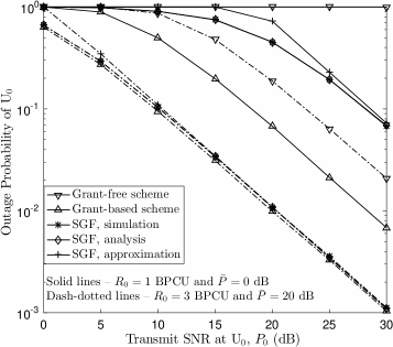
(a) $\tau=0.1$

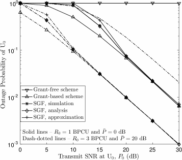
(b) $\tau=\frac{1}{P_{0}}$

Figure 1: Impact of Type I open-loop SGF NOMA transmission on the outage probability of $\text{U}_{0}$. $M=20$. BPCU denotes bit per channel use.

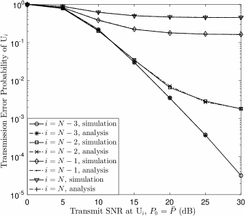
Figure 2: Impact of Type I open-loop SGF NOMA transmission on the transmission error probability of $\text{U}_{i}$. $N=5$, $\tau=0.5$, and $\breve{R}_{i}=0.6$ BPCU.

In Fig. 2, the impact of the open-loop Type I SGF protocol on the grant-free users’ data rates is studied, where it is assumed that there are $N=5$ selected grant-free users. The definition of the transmission errors is based on (10). As can be observed from the figure, the grant-free users’ transmission error probabilities exhibit error floors. This is due to the fact that $\text{U}_{i}$ is impaired by the interference from grant-free users $\text{U}_{j}$, $j<i$. These error floors are reduced by reducing $i$, since $\text{U}_{i}$ is affected by less interference than $\text{U}_{k}$, for $i<k$. Fig. 2 also demonstrates the accuracy of the developed analytical results.

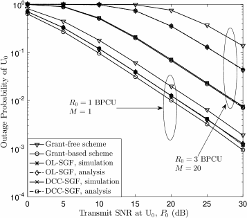
Figure 3: Impact of Type I SGF NOMA transmission on the outage probability of $\text{U}_{0}$ for the open-loop and distributed contention control protocols. $\tau=1$ and $\bar{P}=0$ dB. OL stands for open-loop and DCC stands for distributed contention control.

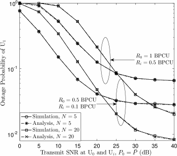
Figure 4: Impact of Type I SGF NOMA transmission with distributed contention control on the outage probability of the grant-free user. $\tau=0.5$.

In Figs. 3 and 4, the performance of the proposed Type I SGF scheme with distributed contention control is evaluated. In Fig. 3, the performance of the Type I SGF scheme is studied for two contention control protocols, open-loop contention control and distributed contention control. When $M=1$, there is no difference between the two protocols, which is the reason why the curves for the two protocols overlap in the figure. For large $M$, distributed contention control ensures that $\text{U}_{0}$ experiences almost the same performance as the grant-based scheme, but fewer grant-free users are scheduled compared to the open-loop scheme. It is worth pointing out that the grant-free scheme results in the worst performance for both cases. Fig. 4 demonstrates the impact of the proposed SGF protocol with distributed contention control on the grant-free user’s outage probability. This figure reveals that there is an error floor, which can be explained as follows. As can be observed from (26), the outage probability $\mathbb{P}_{1}^{\mathrm{I,DCC}}$ comprises two outage events, $\left(\log\left(1+\frac{|h_{0}|^{2}P_{0}}{|h_{(1)}|^{2}\bar{P}+1}\right)>R_{0},\log\left(1+|h_{(1)}|^{2}\bar{P}\right)<R_{i}\right)$ and $\left(\log\left(1+\frac{|h_{0}|^{2}P_{0}}{|h_{(1)}|^{2}\bar{P}+1}\right)<R_{0}\right)$. The event $\left(\log\left(1+\frac{|h_{0}|^{2}P_{0}}{|h_{(1)}|^{2}\bar{P}+1}\right)<R_{0}\right)$ is the cause for the error floor since the SINR becomes a constant when both $P_{0}$ and $\bar{P}$ approach infinity, as shown in (29). This error floor can be reduced by increasing $N$ and reducing the users’ rate requirements. In particular, a large $N$ can reduce the error floor because $|h_{(1)}|^{2}$ is more likely to be small for large $N$ and hence the event $\left(\log\left(1+\frac{|h_{0}|^{2}P_{0}}{|h_{(1)}|^{2}\bar{P}+1}\right)<R_{0}\right)$ is less likely to happen.

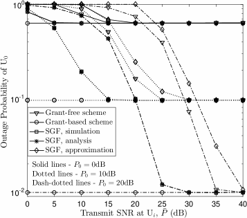
(a) $\mathbb{P}_{0}^{\mathrm{II,OL}}$ for $R_{i}=0.5$ BPCU and $R_{0}=2R_{i}$.

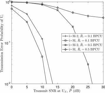
(b) $\mathbb{P}_{i}^{\mathrm{II,OL}}$ for $P_{0}=20$ dB and $N=5$.

Figure 5: Performance of Type II SGF NOMA transmission with open-loop contention control. $M=10$ and $\tau=1$.

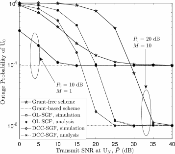
Figure 6: Impact of Type II SGF NOMA transmission on the outage probability of $\mathrm{U}_{0}$ with open-loop contention control and distributed contention control. $\tau=1$, $M=20$, $R_{0}=1$ BPCU and $R_{i}=0.5$ BPCU.

In Figs. 5, 6, and 7, the performance of the proposed Type II SGF protocol is evaluated, where the conventional grant-based and grant-free protocols are used as benchmarks. Fig. 5 demonstrates the impact of the proposed Type II SGF protocol with open-loop contention control on $\mathbb{P}_{0}^{\mathrm{II,OL}}$ and $\mathbb{P}_{i}^{\mathrm{II,OL}}$, respectively. Consistent with Fig. 1, the use of the proposed SGF protocol can ensure that $\text{U}_{0}$ experiences the same outage performance as if it solely occupied $\text{B}_{0}$, while the grant-free scheme realizes the worst performance among the three considered schemes. However, unlike the Type I protocol, the gap between the grant-based and SGF schemes is reduced by increasing $\bar{P}$, as can be observed from Fig. 5(a). The outage probability in Fig. 5(a) has an error floor since the outage probability of the SGF scheme is lower bounded by the outage probability for the grant-based scheme, i.e., $\mathbb{P}(1+|h_{0}|^{2}P_{0}<R_{0})$. Fig. 5(b) shows the interesting phenomenon that $\mathbb{P}_{i}^{\mathrm{II,OL}}$ is smaller than $\mathbb{P}_{j}^{\mathrm{II,OL}}$, for $i>j$, if $\breve{R}_{i}$ is small enough. Otherwise, $\mathbb{P}_{i}^{\mathrm{II,OL}}$ can be larger than $\mathbb{P}_{j}^{\mathrm{II,OL}}$. Characterizing this impact of $\breve{R}_{i}$ on $\mathbb{P}_{i}^{\mathrm{II,OL}}$ by finding a closed-form expression for $\mathbb{P}_{i}^{\mathrm{II,OL}}$ is an important topic for future research.

In Fig. 6, the performances of the proposed Type II SGF schemes with open-loop and distributed contention control are compared. Note that the two control mechanisms become identical if there is only one grant-free user, which is the reason why the curves for the two schemes coincide for $M=1$. By increasing $M$, the open-loop based scheme offers the benefit that more grant-free users are admitted to $\text{B}_{0}$, but the resulting outage performance is worse than that of the scheme with distributed contention control. It is worth pointing out that both schemes outperform the grant-free scheme and achieve the same performance as the grant-based scheme for large $\bar{P}$. In Fig. 7, the impact of the Type II SGF scheme with distributed contention control on the selected grant-free user’s outage performance is studied. As discussed in Remark 11, unlike Type I SGF, the use of Type II SGF can ensure that the outage probability of the grant-free user approaches zero as $\bar{P}$ grows, which is confirmed by the simulation results in Fig. 7.

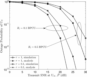
Figure 7: Impact of Type II SGF NOMA transmission with distributed contention control on the outage probability of $\mathrm{U}_{N}$. $P_{0}=30$ dB and $N=5$.

VI Conclusions

In this paper, we have proposed an SGF communication scheme, where one user is granted the right to transmit via a grant based protocol and the other users are admitted to the same channel via a grant-free protocol. Two contention control mechanisms have been proposed to ensure that the number of users admitted to the same channel is carefully controlled. This feature is particularly important for scenarios with an excessive number of active users, where most existing grant-free schemes are not applicable since admitting a large number of users to the same channel can lead to MUD failure. Analytical results and an asymptotic analysis have been provided to demonstrate the superior performance of the proposed NOMA assisted SGF schemes and to study the impact of different SIC decoding orders. In particular, the proposed Type I SGF schemes are ideally suited for the scenario, where the grant-based user is close to the base station and the grant-free users are cell-edge users. On the other hand, the proposed Type II SGF schemes are ideal for the scenario, where the grant-based user is a cell-edge user and the grant-free users are close to the base station. In this paper, each user is assumed to know its CSI perfectly. An important topic for future research is the study of the impact of imperfect CSI on the design of SGF schemes.

Appendix A Proof for Theorem 1

By using order statistics [24], $\mathbb{P}(N=n)$ can be obtained as follows:

$$\mathbb{P}(N=n)= \mathbb{P}\left(|h_{(n)}|^{2}<\tau,|h_{(n+1)}|^{2}>\tau\right)$$ (49)

$$= \frac{M!}{n!(M-n)!}e^{-(M-n)\tau}\left(1-e^{-\tau}\right)^{n},$$

for $1\leq n\leq(M-1)$. It is straightforward to show that the expression in (49) is also valid for the case $n=M$. The remainder of the proof focuses on the calculation of $Q_{1}$ in (2), the outage probability conditioned on $N=n$.

$Q_{1}$ can be first rewritten as follows:

$$Q_{1}= \mathbb{P}\left(\left.\sum^{n}_{j=1}|h_{(j)}|^{2}>\frac{|h_{0}|^{2}P_{0}\bar{P}^{-1}}{2^{R_{0}}-1}-\bar{P}^{-1}\right|N=n\right).$$ (50)

The pdf of $\sum^{n}_{j=1}|h_{(j)}|^{2}$ can be found by treating it as the sum of the $n$ smallest order statistics among the $M$ channel gains [25]. Since all $|h_{(j)}|^{2}$, $1\leq j\leq n$, are smaller than $\tau$, a simple alternative is to treat $\sum^{n}_{j=1}|h_{(j)}|^{2}$ as the sum of $n$ i.i.d. variables, denoted by $|\tilde{h}_{j}|^{2}$ with the following CDF:

$$F_{|\tilde{h}_{j}|^{2}}(y)=\left\{\begin{array}[]{ll}\frac{1-e^{-y}}{1-e^{-\tau}},&\text{if}\quad y\leq\tau\\ 1,&\text{if}\quad y>\tau\end{array}\right..$$ (53)

The pdf of $|\tilde{h}_{j}|^{2}$, denoted by $f_{|\tilde{h}_{j}|^{2}}(y)$, can be obtained straightforwardly. The Laplace transform of $f_{|\tilde{h}_{j}|^{2}}(y)$ is given by

$$\mathcal{L}\left(f_{|\tilde{h}_{j}|^{2}}(y)\right)=\frac{1-e^{-(s+1)\tau}}{(s+1)(1-e^{-\tau})}.$$ (54)

Since the $|\tilde{h}_{j}|^{2}$ are i.i.d., the Laplace transform of the pdf of $\sum^{n}_{j=1}|\tilde{h}_{j}|^{2}$ is given by

$$\mathcal{L}\left(f_{\sum^{n}_{j=1}|\tilde{h}_{j}|^{2}}(y)\right)= \frac{\left(1-e^{-(s+1)\tau}\right)^{n}}{(s+1)^{n}(1-e^{-\tau})^{n}}$$ (55)

$$= \sum^{n}_{p=0}\frac{{n\choose p}(-1)^{p}e^{-p\tau}}{(1-e^{-\tau})^{n}}\frac{e^{-p\tau s}}{(s+1)^{n}}.$$

By applying the inverse Laplace transform and also using the fact that $\sum^{n}_{j=1}|\tilde{h}_{j}|^{2}$ and $\sum^{n}_{j=1}|{h}_{(j)}|^{2}$ have the same pdf, the pdf of $\sum^{n}_{j=1}|{h}_{(j)}|^{2}$ is obtained as follows:

$$f_{\sum^{n}_{j=1}|{h}_{(j)}|^{2}}(y)= \mathcal{L}^{-1}\left(\sum^{n}_{p=0}\frac{{n\choose p}(-1)^{p}e^{-p\tau}}{(1-e^{-\tau})^{n}}\frac{e^{-p\tau s}}{(s+1)^{n}}\right)$$

$$= \sum^{n}_{p=0}\frac{{n\choose p}(-1)^{p}e^{-p\tau}}{(1-e^{-\tau})^{n}(n-1)!}(y-p\tau)^{n-1}e^{-(y-p\tau)}u(y-p\tau).$$ (56)

Intuitively, $f_{\sum^{n}_{j=1}|{h}_{(j)}|^{2}}(y)=0$ for $y\geq n\tau$, since $|{h}_{(j)}|^{2}<\tau$ for $1\leq j\leq n$. Because the pdf expression in (56) contains the step function, it is not straightforward to show that this expression fits the intuition. Thus, we verify this result in the following lemma.

$\mathbf{Lemma}$ 2.

The expression for the pdf of $\sum^{n}_{j=1}|{h}_{(j)}|^{2}$ in (56) has the following property:

$$f_{\sum^{n}_{j=1}|{h}_{(j)}|^{2}}(y)=0,$$ (57)

for $y\geq n\tau$.

Proof.

See Appendix B. ∎

By using $f_{\sum^{n}_{j=1}|{h}_{(j)}|^{2}}(y)$, probability $Q_{1}$ can be expressed as follows:

$$Q_{1}= \int^{\infty}_{\epsilon_{0}P_{0}^{-1}}\int_{\epsilon_{x}}^{\infty}f_{\sum^{n}_{j=1}|{h}_{(j)}|^{2}}(y)dyf_{|h_{0}|^{2}}(x)dx+\int^{\epsilon_{0}P_{0}^{-1}}_{0}f_{|h_{0}|^{2}}(x)dx$$ (58)

$$= \sum^{n}_{p=0}\frac{{n\choose p}(-1)^{p}e^{-p\tau}}{(1-e^{-\tau})^{n}(n-1)!}\int^{\infty}_{\epsilon_{0}P_{0}^{-1}}\int_{\epsilon_{x}}^{\infty}(y-p\tau)^{n-1}$$

$$\times e^{-(y-p\tau)}u(y-p\tau)dyf_{|h_{0}|^{2}}(x)dx+1-e^{-\epsilon_{0}P_{0}^{-1}},$$

where $\epsilon_{x}=\frac{xP_{0}\bar{P}^{-1}}{2^{R_{0}}-1}-\bar{P}^{-1}$. Define $\bar{\epsilon}_{x}=(\epsilon_{x}-p\tau)^{+}$, where $(x)^{+}\triangleq\max(0,x)$.

Note that the upper end of the integration range for $\sum^{n}_{j=1}|{h}_{(j)}|^{2}$ should be $n\tau$ since each ${h}_{(j)}$ is upper bounded by $\tau$, but can be replaced by $\infty$ because of Lemma 2. Therefore, $Q_{1}$ can be evaluated as follows:

$$Q_{1}= \sum^{n}_{p=0}\frac{{n\choose p}(-1)^{p}e^{-p\tau}}{(1-e^{-\tau})^{n}(n-1)!}\int^{\infty}_{\epsilon_{0}P_{0}^{-1}}\int_{\bar{\epsilon}_{x}}^{\infty}x^{n-1}e^{-x}dy$$

$$\times f_{|h_{0}|^{2}}(x)dx+1-e^{-\epsilon_{0}P_{0}^{-1}}$$

$$\overset{(b)}{=}\sum^{n}_{p=0}\frac{{n\choose p}(-1)^{p}e^{-p\tau}}{(1-e^{-\tau})^{n}(n-1)!}\int^{\infty}_{\epsilon_{0}P_{0}^{-1}}\Gamma(n,\bar{\epsilon}_{x})f_{|h_{0}|^{2}}(x)dx+1-e^{-\epsilon_{0}P_{0}^{-1}},$$ (59)

where step $(b)$ follows [26, Eq. (3.38.3)] and $\Gamma(\cdot)$ denotes the upper incomplete Gamma function. By using the series expansion of the Gamma function [26], $Q_{1}$ can be expressed as follows:

$$Q_{1}= 1-e^{-\epsilon_{0}P_{0}^{-1}}+\sum^{n}_{p=0}\frac{{n\choose p}(-1)^{p}e^{-p\tau}}{(1-e^{-\tau})^{n}(n-1)!}\sum_{l=0}^{n-1}\frac{(n-1)!}{l!}$$ (60)

$$\times\int^{\infty}_{\epsilon_{0}P_{0}^{-1}}\left[\left(\frac{xP_{0}\bar{P}^{-1}}{2^{R_{0}}-1}-\bar{P}^{-1}-p\tau\right)^{+}\right]^{l}e^{-(x+\bar{\epsilon}_{x})}dx$$

$$= 1-e^{-\epsilon_{0}P_{0}^{-1}}+\sum^{n}_{p=0}\frac{{n\choose p}(-1)^{p}e^{-p\tau}}{(1-e^{-\tau})^{n}(n-1)!}\sum_{l=0}^{n-1}\frac{(n-1)!}{l!}$$

$$\times\int^{\infty}_{\epsilon_{0}P_{0}^{-1}}\left[\left(\frac{x-\epsilon_{0}P_{0}^{-1}-\epsilon_{0}P_{0}^{-1}\bar{P}p\tau}{\epsilon_{0}P_{0}^{-1}\bar{P}}\right)^{+}\right]^{l}e^{-(x+\bar{\epsilon}_{x})}dx.$$

The expression for $Q_{1}$ can be further simplified as follows:

$$Q_{1}=1-e^{-\epsilon_{0}P_{0}^{-1}}+\sum^{n}_{p=0}\frac{{n\choose p}(-1)^{p}e^{-p\tau}}{(1-e^{-\tau})^{n}(n-1)!}\left(\sum_{l=0}^{n-1}\frac{(n-1)!}{l!}\right.$$

$$\times\underset{Q_{11}}{\underbrace{\int^{\infty}_{\epsilon_{0}P_{0}^{-1}+\epsilon_{0}P_{0}^{-1}\bar{P}p\tau}\left[\frac{x-\epsilon_{0}P_{0}^{-1}-\epsilon_{0}P_{0}^{-1}\bar{P}p\tau}{\epsilon_{0}P_{0}^{-1}\bar{P}}\right]^{l}e^{-(x+\bar{\epsilon}_{x})}dx}}$$

$$\left.+\underset{Q_{12}}{\underbrace{(n-1)!\int_{\epsilon_{0}P_{0}^{-1}}^{\epsilon_{0}P_{0}^{-1}+\epsilon_{0}P_{0}^{-1}\bar{P}p\tau}e^{-x}dx}}\right),$$

where the integral range in $Q_{11}$ is reduced since $\epsilon_{0}P_{0}^{-1}+\epsilon_{0}P_{0}^{-1}\bar{P}p\tau>\epsilon_{0}P_{0}^{-1}$ and $\left(\frac{x-\epsilon_{0}P_{0}^{-1}-\epsilon_{0}P_{0}^{-1}\bar{P}p\tau}{\epsilon_{0}P_{0}^{-1}\bar{P}}\right)^{+}=0$ if $x<\epsilon_{0}P_{0}^{-1}+\epsilon_{0}P_{0}^{-1}\bar{P}p\tau$. $Q_{12}$ in the above equation is needed due to the fact that, for the special case of $l=0$, the integral is not zero even if $\bar{\epsilon}_{x}=0$.

By applying [26, Eq. (3.381.4)], $Q_{1}$ can be expressed as follows:

$$Q_{1}= \sum^{n}_{p=0}\frac{{n\choose p}(-1)^{p}e^{-p\tau}}{(1-e^{-\tau})^{n}(n-1)!}\left(\sum_{l=0}^{n-1}\frac{(n-1)!}{l!}\right.$$ (61)

$$\times\left.\frac{e^{-\epsilon_{0}P_{0}^{-1}(1+\bar{P}p\tau)}l!}{\epsilon_{0}^{l}P_{0}^{-l}\bar{P}^{l}(1+\epsilon_{0}^{-1}P_{0}\bar{P}^{-1})^{(l+1)}}+(n-1)!\left(e^{-\epsilon_{0}P_{0}^{-1}}-e^{-\epsilon_{0}P_{0}^{-1}(1+\bar{P}p\tau)}\right)\right)+1-e^{-\epsilon_{0}P_{0}^{-1}}.$$

Therefore, the outage probability of $\text{U}_{0}$ can be obtained as follows:

$$\mathbb{P}_{0}^{\mathrm{I,OL}}= \sum_{n=1}^{M}\frac{M!e^{-(M-n)\tau}\left(1-e^{-\tau}\right)^{n}}{n!(M-n)!}\left(\sum^{n}_{p=0}\frac{{n\choose p}(-1)^{p}e^{-p\tau}}{(1-e^{-\tau})^{n}}\right.$$

$$\times\left.\left(\sum_{l=0}^{n-1}\frac{e^{-\epsilon_{0}P_{0}^{-1}(1+\bar{P}p\tau)}}{\epsilon_{0}^{l}P_{0}^{-l}\bar{P}^{l}(1+\epsilon_{0}^{-1}P_{0}\bar{P}^{-1})^{(l+1)}}\right.\right.$$

$$\left.\left.+e^{-\epsilon_{0}P_{0}^{-1}}-e^{-\epsilon_{0}P_{0}^{-1}(1+\bar{P}p\tau)}\right)+1-e^{-\epsilon_{0}P_{0}^{-1}}\right)$$

$$+e^{-M\tau}\left(1-e^{-\epsilon_{0}P_{0}^{-1}}\right).$$ (62)

Note that

$$\sum_{n=1}^{M}\frac{M!}{n!(M-n)!}e^{-(M-n)\tau}\left(1-e^{-\tau}\right)^{n}+e^{-M\tau}=1.$$ (63)

By applying (63) to (62), the expression for $\mathbb{P}_{0}^{\mathrm{I,OL}}$ can be simplified as shown in the theorem, and the proof is complete.

Appendix B Proof for Lemma 2

The lemma can be proved by first rewriting the pdf as follows:

$$f_{\sum^{n}_{j=1}|{h}_{j}|^{2}}(y)= \frac{e^{-y}}{(1-e^{-\tau})^{n}(n-1)!}\sum^{n}_{p=0}{n\choose p}(-1)^{p}$$ (64)

$$\times(y-p\tau)^{n-1}u(y-p\tau).$$

In the case of $y\geq n\tau$, $u(y-p\tau)=1$, which means that the pdf can be simplified as follows:

$$f_{\sum^{n}_{j=1}|{h}_{j}|^{2}}(y)= \frac{e^{-y}}{(1-e^{-\tau})^{n}(n-1)!}\sum^{n}_{p=0}{n\choose p}(-1)^{p}\sum^{n-1}_{l=0}y^{n-1-l}(-1)^{l}p^{l}$$ (65)

$$= \frac{e^{-y}}{(1-e^{-\tau})^{n}(n-1)!}\sum^{n-1}_{l=0}y^{n-1-l}\sum^{n}_{p=0}{n\choose p}(-1)^{p}(-1)^{l}p^{l}.$$

It is important to point out that $l$ is strictly smaller than $n$. According to in [26, Eq. (0.154.3)], we have

$$\sum^{n}_{p=0}{n\choose p}(-1)^{p}(-1)^{l}p^{l}=0,$$ (66)

for $l<n$. Therefore $f_{\sum^{n}_{j=1}|{h}_{j}|^{2}}(y)=0$, for $y\geq n\tau$. This completes the proof.

Appendix C Proof for Theorem 2

The first step of the proof is to find $\mathbb{P}(N=n)$, which can be expressed as follows:

$$\mathbb{P}(N=n)=\mathbb{P}\left(|h_{(M-n)}|^{2}<\tau,|h_{(M-n+1)}|^{2}>\tau\right).$$ (67)

Note that (67) is different from (49). By applying order statistics, the outage probability can be expressed as follows:

$$\mathbb{P}_{0}^{\mathrm{II,OL}}= 1-\sum^{M}_{n=1}\frac{M!}{n!(M-n)!}e^{-n\tau}\left(1-e^{-\tau}\right)^{M-n}Q_{3}$$ (68)

$$-\left(1-e^{-\tau}\right)^{M}e^{-\epsilon_{0}P_{0}^{-1}}.$$

The remainder of the proof is to find an expression for $Q_{3}$. With some algebraic manipulations, $Q_{3}$ can be expressed as follows:

$$Q_{3}= \underset{|h_{0}|^{2}>\frac{\epsilon_{0}}{P_{0}}}{\mathcal{E}}\left\{\mathbb{P}\left(\left.y_{n}>\epsilon_{s,n}\bar{P}^{-1}(1+P_{0}|h_{0}|^{2})\right|N=n\right)\right\},$$ (69)

where $\mathcal{E}\{\cdot\}$ denotes the expectation operation, and $y_{n}=\sum^{M}_{j=M-n+1}|h_{(j)}|^{2}$.

By applying order statistics, one can evaluate $Q_{3}$ by using the distribution of the sum of the $n$ largest order statistics among $M$ Rayleigh fading gains. However, a simpler alternative is to treat $y_{n}$ as the sum of $n$ i.i.d. random variables, denoted by $\tilde{g}_{j}$, with the following CDF:

$$F_{|\tilde{g}_{j}|^{2}}(y)=\left\{\begin{array}[]{ll}0,&\text{if}\quad y\leq\tau\\ \frac{e^{-\tau}-e^{-y}}{e^{-\tau}},&\text{if}\quad y>\tau\end{array}\right.,$$ (72)

which is different from (53) since $|\tilde{g}_{j}|^{2}\geq\tau$ and $|\tilde{h}_{j}|^{2}\leq\tau$. The pdf of $|\tilde{g}_{j}|^{2}$, $f_{|\tilde{g}_{j}|^{2}}(y)$, can be obtained straightforwardly. The Laplace transform of $f_{|\tilde{g}_{j}|^{2}}(y)$ is given by

$$\mathcal{L}\left(f_{|\tilde{g}_{j}|^{2}}(y)\right)=\frac{e^{-s\tau}}{s+1}.$$ (73)

Since the $|\tilde{g}_{j}|^{2}$ are i.i.d., the Laplace transform of the pdf of $y_{n}$ can be found as follows:

$$\mathcal{L}\left(f_{y_{n}}(y)\right)=\frac{e^{-n\tau s}}{(s+1)^{n}},$$ (74)

which yields the following expression for the pdf of $y_{n}$

$$f_{y_{n}}(y)=\frac{(y-n\tau)^{n-1}e^{-(y-n\tau)}u(y-n\tau)}{(n-1)!}.$$ (75)

As a result, $Q_{3}$ can be calculated as follow:

$$Q_{3}= \underset{|h_{0}|^{2}>\epsilon_{0}P_{0}^{-1}}{\mathcal{E}}\left\{\int_{\epsilon_{s,n}\bar{P}^{-1}(1+P_{0}|h_{0}|^{2})}^{\infty}f_{y_{n}}(y)dy\right\}$$ (76)

$$= \underset{|h_{0}|^{2}>\epsilon_{0}P_{0}^{-1}}{\mathcal{E}}\left\{\int_{(\Delta_{h}-n\tau)^{+}}^{\infty}\frac{z^{n-1}e^{-z}}{(n-1)!}dy\right\}=\underset{|h_{0}|^{2}>\epsilon_{0}P_{0}^{-1}}{\mathcal{E}}\left\{\frac{\Gamma(n,(\Delta_{h}-n\tau)^{+})}{(n-1)!}\right\},$$

where $\Delta_{h}=\epsilon_{s,n}\bar{P}^{-1}(1+P_{0}|h_{0}|^{2})$.

Next, by applying the series expression of the incomplete Gamma function [26], we obtain the following:

$$Q_{3}= \underset{|h_{0}|^{2}>\epsilon_{0}P_{0}^{-1}}{\mathcal{E}}\left\{e^{-(\Delta_{h}-n\tau)^{+}}\sum^{n-1}_{l=0}\frac{\left[(\Delta_{h}-n\tau)^{+}\right]^{l}}{l!}\right\}$$ (77)

$$= \int^{\infty}_{\epsilon_{0}P_{0}^{-1}}e^{-\epsilon_{s,n}\bar{P}^{-1}P_{0}\left(x-\frac{n\tau\epsilon_{s,n}^{-1}\bar{P}-1}{P_{0}}\right)^{+}}\sum^{n-1}_{l=0}\frac{\epsilon_{s,n}^{l}\bar{P}^{-l}P_{0}^{l}}{l!}\left[\left(x-\frac{n\tau\epsilon_{s,n}^{-1}\bar{P}-1}{P_{0}}\right)^{+}\right]^{l}e^{-x}dx.$$

Similar to the proof for Theorem 1, the result for the case $l=0$ needs to be calculated separately as follows:

$$Q_{3}= \int^{\infty}_{\epsilon_{0}P_{0}^{-1}}e^{-\epsilon_{s,n}\bar{P}^{-1}P_{0}\left(x-\frac{n\tau\epsilon_{s,n}^{-1}\bar{P}-1}{P_{0}}\right)^{+}}\sum^{n-1}_{l=1}\frac{\epsilon_{s,n}^{l}\bar{P}^{-l}P_{0}^{l}}{l!}\left[\left(x-\frac{n\tau\epsilon_{s,n}^{-1}\bar{P}-1}{P_{0}}\right)^{+}\right]^{l}e^{-x}dx$$

$$+\int^{\infty}_{\epsilon_{0}P_{0}^{-1}}e^{-\epsilon_{s,n}\bar{P}^{-1}P_{0}\left(x-\frac{n\tau\epsilon_{s,n}^{-1}\bar{P}-1}{P_{0}}\right)^{+}}e^{-x}dx.$$ (78)

Since $\tau_{n}$ is not necessarily larger than $\epsilon_{0}P_{0}^{-1}$, we introduce $\tau_{n}$ and $\bar{\tau}_{n}$ as defined in the theorem and $Q_{3}$ can be calculated as follows:

$$Q_{3}= \int^{\infty}_{\bar{\tau}_{n}}e^{-\epsilon_{s,n}\bar{P}^{-1}P_{0}\left(x-\tau_{n}\right)}\sum^{n-1}_{l=1}\frac{\epsilon_{s,n}^{l}\bar{P}^{-l}P_{0}^{l}}{l!}\left[x-\tau_{n}\right]^{l}e^{-x}dx$$

$$+\int^{\bar{\tau}_{n}}_{\epsilon_{0}P_{0}^{-1}}e^{-x}dx+\int^{\infty}_{\bar{\tau}_{n}}e^{-\epsilon_{s,n}\bar{P}^{-1}P_{0}\left(x-\tau_{n}\right)}e^{-x}dx$$

$$= \sum^{n-1}_{l=1}\frac{\epsilon_{s,n}^{l}\bar{P}^{-l}P_{0}^{l}}{l!}e^{-\tau_{n}}\frac{\Gamma\left(l+1,(\bar{\tau}_{n}-\tau_{n})(1+\epsilon_{s,n}\bar{P}^{-1}P_{0})\right)}{(1+\epsilon_{s,n}\bar{P}^{-1}P_{0})^{l+1}}$$

$$+e^{-\epsilon_{0}P_{0}^{-1}}-e^{-\bar{\tau}_{n}}+\frac{e^{-\tau_{n}-(\bar{\tau}_{n}-\tau_{n})(1+\epsilon_{s,n}\bar{P}^{-1}P_{0})}}{1+\epsilon_{s,n}\bar{P}^{-1}P_{0}}.$$ (79)

By substituting (79) into (68), the closed-form expression for $\mathbb{P}_{0}^{\mathrm{II,OL}}$ can be obtained and the proof is complete.

References

• [1] M. Shafi, A. F. Molisch, P. J. Smith, T. Haustein, P. Zhu, P. D. Silva, F. Tufvesson, A. Benjebbour, and G. Wunder, “5G: A tutorial overview of standards, trials, challenges, deployment, and practice,” IEEE J. Sel. Areas Commun., vol. 35, no. 6, pp. 1201–1221, Jun. 2017.
• [2] Z. Ding, Y. Liu, J. Choi, Q. Sun, M. Elkashlan, C.-L. I, and H. V. Poor, “Application of non-orthogonal multiple access in LTE and 5G networks,” IEEE Commun. Mag., vol. 55, no. 2, pp. 185–191, Feb. 2017.
• [3] Z. Ding, X. Lei, G. K. Karagiannidis, R. Schober, J. Yuan, and V. Bhargava, “A survey on non-orthogonal multiple access for 5G networks: Research challenges and future trends,” IEEE J. Sel. Areas Commun., vol. 35, no. 10, pp. 2181–2195, Oct. 2017.
• [4] M. Al-Imari, P. Xiao, M. A. Imran, and R. Tafazolli, “Uplink non-orthogonal multiple access for 5G wireless networks,” in Proc. 11th Int. Symposium on Wireless Commun. Systems (ISWCS), Barcelona, Spain, Aug 2014, pp. 781–785.
• [5] M. S. Ali, H. Tabassum, and E. Hossain, “Dynamic user clustering and power allocation for uplink and downlink non-orthogonal multiple access (NOMA) systems,” IEEE Access, vol. 4, pp. 6325–6343, 2016.
• [6] Y. Sun, D. W. K. Ng, Z. Ding, and R. Schober, “Optimal joint power and subcarrier allocation for full-duplex multicarrier non-orthogonal multiple access systems,” IEEE Trans. Commun., vol. 65, no. 3, pp. 1077–1091, Mar. 2017.
• [7] H. Chen, R. Abbas, P. Cheng, M. Shirvanimoghaddam, W. Hardjawana, W. Bao, Y. Li, and B. Vucetic, “Ultra-reliable low latency cellular networks: Use cases, challenges and approaches,” to appear in 2018.
• [8] X. Sun, S. Yan, N. Yang, Z. Ding, C. Shen, and Z. Zhong, “Short-packet downlink transmission with non-orthogonal multiple access,” IEEE Trans. Wireless Commun., vol. 17, no. 7, pp. 4550–4564, Jul. 2018.
• [9] M. Bennis, M. Debbah, and H. V. Poor, “Ultra-reliable and low-latency communication: Tail, risk and scale,” Proceedings of the IEEE, to appear in 2018.
• [10] “5G, a techology vision,” Huawei, Inc., Shengzheng, China, 5G Whitepaper, Mar. 2015.
• [11] X. Bian, J. Tang, H. Wang, M. Li, and R. Song, “An uplink transmission scheme for pattern division multiple access based on DFT spread generalized multi-carrier modulation,” IEEE Access, vol. 6, pp. 34 135–34 148, 2018.
• [12] G. Ma, B. Ai, F. Wang, X. Chen, Z. Zhong, Z. Zhao, and H. Guan, “Coded tandem spreading multiple access for massive machine-type communications,” IEEE Wireless Commun., vol. 25, no. 2, pp. 75–81, Apr. 2018.
• [13] L. Liu and W. Yu, “Massive connectivity with massive MIMO - Part I: Device activity detection and channel estimation,” IEEE Trans. on Signal Process., vol. 66, no. 11, pp. 2933–2946, Jun. 2018.
• [14] ——, “Massive connectivity with massive MIMO - Part II: Achievable rate characterization,” IEEE Trans. Signal Process., vol. 66, no. 11, pp. 2947–2959, Jun. 2018.
• [15] Y. Du, C. Cheng, B. Dong, Z. Chen, X. Wang, J. Fang, and S. Li, “Block-sparsity-based multiuser detection for uplink grant-free NOMA,” IEEE Trans. Wireless Commu., to appear in 2018.
• [16] M. Shirvanimoghaddam, M. Condoluci, M. Dohler, and S. J. Johnson, “On the fundamental limits of random non-orthogonal multiple access in cellular massive IoT,” IEEE J. Sel. Topics Signal Process., vol. 35, no. 10, pp. 2238–2252, Oct. 2017.
• [17] J. Choi, “NOMA based random access with multichannel ALOHA,” IEEE J. Sel. Areas Commun., vol. PP, no. 99, pp. 1–1, 2017.
• [18] P. Viswanath, D. Tse, and R. Laroia, “Opportunistic beamforming using dumb antennas,” IEEE Trans. Inform. Theory, vol. 48, pp. 1277– 1294, Jun. 2003.
• [19] Z. Ding, P. Fan, and H. V. Poor, “Random beamforming in millimeter-wave NOMA networks,” IEEE Access, vol. 5, pp. 7667–7681, 2017.
• [20] Q. Zhao and L. Tong, “Opportunistic carrier sensing for energy-efficient information retrieval in sensor networks,” EURASIP Journal on Wireless Communications and Networking, vol. 2, no. 2, pp. 1–1, Apr. 2005.
• [21] A. Bletsas, A. Khisti, D. P. Reed, and A. Lippman, “A simple cooperative diversity method based on network path selection,” IEEE Journal Select. Areas in Comm., vol. 24, pp. 659–672, Mar. 2006.
• [22] R. Talak and N. B. Mehta, “Feedback overhead-aware, distributed, fast, and reliable selection,” IEEE Trans. Commu., vol. 60, no. 11, pp. 3417–3428, Nov. 2012.
• [23] Z. Ding, P. Fan, and H. V. Poor, “Impact of user pairing on 5G non-orthogonal multiple access,” IEEE Trans. Veh. Tech., vol. 65, no. 8, pp. 6010–6023, Aug. 2016.
• [24] H. A. David and H. N. Nagaraja, Order Statistics.   John Wiley, New York, 3rd ed., 2003.
• [25] K. Alam and K. T. Wallenius, “Distribution of a sum of order statistics,” Scandinavian Journal of Statistics, vol. 6, no. 3, pp. 123–126, 1979.
• [26] I. S. Gradshteyn and I. M. Ryzhik, Table of Integrals, Series and Products, 6th ed.   New York: Academic Press, 2000.