Update on $B\to D^{\ast}\ell\nu$ form factor at zero-recoil using the Oktay-Kronfeld action

Abstract:

We present an update on the calculation of $\bar{B}\to D^{\ast}\ell\bar{\nu}$ semileptonic form factor at zero recoil using the Oktay-Kronfeld bottom and charm quarks on $N_{f}=2+1+1$ flavor HISQ ensembles generated by the MILC collaboration. Preliminary results are given for two ensembles with $a\approx 0.12$ and $0.09$ fm and $M_{\pi}\approx 310$ MeV. Calculations have been done with a number of valence quark masses, and the dependence of the form factor on them is investigated on the $a\approx 0.12\,\,\mathrm{fm}$ ensemble. The excited state is controlled by using multistate fits to the three-point correlators measured at 4–6 source-sink separations.

1 Introduction

Lattice calculation of $\bar{B}\rightarrow D^{\ast}\ell\bar{\nu}$ semileptonic decay form factors can be used to determine the CKM matrix element $|V_{cb}|$ from the measured exclusive decay rates. Precise results for exclusive $|V_{cb}|$ will address the well-known $\approx 3\sigma$ discrepancy from the inclusive determination of $|V_{cb}|$ [1]. In addition, there is an analysis showing $\approx 4\sigma$ tension in the standard model evaluation of $|\varepsilon_{K}|$ [2] using the exclusive $|V_{cb}|$.

For the $\bar{B}\rightarrow D^{\ast}\ell\bar{\nu}$ study, the heavy quark discretization error, estimated by HQET power counting in terms of $\displaystyle\lambda_{c}\sim\frac{\Lambda_{QCD}}{2m_{c}}\sim\frac{500~{}\text{MeV}}{2\times 1.3~{}\text{GeV}}\sim\frac{1}{5}$, is dominant especially for charm. Calculations of the zero recoil form factor $\mathcal{F}(w=1)=h_{A_{1}}(1)$ using the Fermilab action has ${\cal O}(\lambda^{3}_{c})\sim 1\%$ uncertainty assuming $\alpha_{s}\sim\lambda_{c}$. To achieve precision below 1% in $|V_{cb}|$, we propose to use the Oktay-Kronfeld (OK) action, in which the discretization error are ${\cal O}(\lambda^{4}_{c})\sim 0.2\%$ provided a full one-loop improvement of correction terms is carried out [3, 4]. In this work, we are working with tree-level tadpole-improvement of the action and current operators since the one-loop calculations are not complete.

We calculate the form factor $h_{A_{1}}(1)$ using the double ratio of ground state matrix elements [5],

$$|{h_{A_{1}}(1)}|^{2}=\frac{\langle D^{\ast}|A^{j}_{cb}|\bar{B}\rangle\langle\bar{B}|A^{j}_{bc}|D^{\ast}\rangle}{\langle D^{\ast}|V^{4}_{cc}|D^{\ast}\rangle\langle\bar{B}|V^{4}_{bb}|\bar{B}\rangle}\times\rho_{A_{j}}^{2}\,,\quad{\rm with}\quad\rho^{2}_{A_{j}}=\frac{Z_{A_{j}}^{cb}Z_{A_{j}}^{bc}}{Z_{V_{4}}^{cc}Z_{V_{4}}^{bb}}\,.$$ (1)

$\rho^{2}_{A_{j}}$ is the matching factor that is expected to be close to unity [5]. Each of the matrix element is extracted from the related three-point function calculated on the lattice. For example, $\langle D^{\ast}|A^{j}_{cb}|B\rangle$ is from $C^{B\rightarrow D^{\ast}}_{A_{1}}(t,\tau)$ defined in Eq. (3). We also use an improved current operator $A_{j}^{cb}(y)=\bar{\Psi}_{c}(y)\gamma_{j}\gamma_{5}\Psi_{b}(y)$ where the improved field $\Psi(x)$ is obtained by the following field rotation on the unimproved fermion field $\psi(x)$: $\Psi(x)=[1+\sum_{i}d_{i}{\cal R}_{i}]\psi(x)$. Improvement up to ${\cal O}(\lambda^{3})$ can be obtained using tree-level matching of the coefficients $d_{i}$ and operators ${\cal R}_{i}$ [6, 7].

We present an update on our previous calculation of $|h_{A_{1}}(1)/\rho_{A_{j}}|$ [8], paying attention to controlling the excited-state contamination (ESC) using multistate fits to 3-point (3pt) data with 4–6 source-sink time separations. The parameters in the calculation on the two $N_{f}=2+1+1$ HISQ ensembles, generated by the MILC collaboration [9], are given in Table 1. The light quark propagators ($u,d,s$) are calculated using the HISQ action with point source and sink. For the heavy quark ($c,b$) propagators, we use the OK action with covariant Gaussian smearing at both the source and the sink. The hopping parameters $\kappa_{\text{crit}}$, $\kappa_{b}$, $\kappa_{c}$ have been tuned nonperturbatively as described in Ref. [8].

ID	$a$	$M_{\pi}$	$m_{x}/m_{s}$	$\kappa_{\text{crit}}$	$\kappa_{c}$	$\kappa_{b}$	$\{\sigma,N_{\text{cvg}}\}$	$N_{\text{cfg}}\times N_{\text{src}}$	$\tau$
$a12m310$	$0.1207$	305	0.1, $0.2^{\dagger}$,	0.051211	0.048524	0.04102	$\{1.5,5\}$	$1053\times 3$	10, 11, 12,
			0.3, 0.4, 1.0						13, 14, 15
$a09m310$	$0.0888$	313	$0.2^{\dagger}$, 1.0	0.05075	0.04894	0.0429	$\{2,10\}$	$1001\times 3$	15, 16, 17, 18

Table 1: Parameters used in the measurements performed on two MILC HISQ gauge ensembles described in Ref. [9]. $m_{x}/m_{s}$ is the ratio of valence spectator quark mass to the sea strange quark mass where $\dagger$ denotes the unitary point for the degenerate up and down quarks. Hopping parameters $\kappa_{\text{crit}}$, $\kappa_{c}$ and $\kappa_{b}$ give the values obtained for the critical and the charm and the bottom quark masses. $\{\sigma,N_{\text{cvg}}\}$ are parameters for the covariant Gaussian smearing. $N_{\text{cfg}}\times N_{\text{src}}$ denotes the number of measurements made. $\tau$ gives the source-sink time separations simulated.

2 Controlling excited-state contamination

To achieve sub-percent precision, we have to control the ESC. On a lattice with time extent $T$, the $B$- and $D^{\ast}$-meson 2-point (2pt) functions, $C^{\text{2pt}}(t)$, are fit using a $3+2$-state ansatz:

$$C^{\text{2pt}}(t)=\langle O^{\dagger}(t)O(0)\rangle ={|\mathcal{A}_{0}|^{2}}e^{-{M_{0}}t}\Big{(}1+{\left|\frac{\mathcal{A}_{2}}{\mathcal{A}_{0}}\right|^{2}}e^{-{\Delta M_{2}}t}+{\left|\frac{\mathcal{A}_{4}}{\mathcal{A}_{0}}\right|^{2}}e^{-{(\Delta M_{2}+\Delta M_{4})}t}+\cdots$$ (2)

$$-(-1)^{t}{\left|\frac{\mathcal{A}_{1}}{\mathcal{A}_{0}}\right|^{2}}e^{-{\Delta M_{1}}t}-(-1)^{t}{\left|\frac{\mathcal{A}_{3}}{\mathcal{A}_{0}}\right|^{2}}e^{-{(\Delta M_{1}+\Delta M_{3})}t}+\cdots\Big{)}+(t\leftrightarrow T-t).$$

where $O$ is the meson interpolating operator. $\Delta M_{n}\equiv M_{n}-M_{n-2}$ with $n=2,4$ are the mass gaps for even parity, and $\Delta M_{1}\equiv M_{1}-M_{0}$ and $\Delta M_{3}\equiv M_{3}-M_{1}$ for the two odd parity states that arise in staggered formulations. An empirical Bayesian method is used to fix the priors for the excited-state masses $M_{n}$ and amplitudes $\mathcal{A}_{n}=\langle n|O|\Omega\rangle$ to stabilize the fits as described in Ref. [10]. Fig. 1 illustrates the results for the ground- and excited-state masses of $D^{\ast}$ meson and the priors used for excited states.

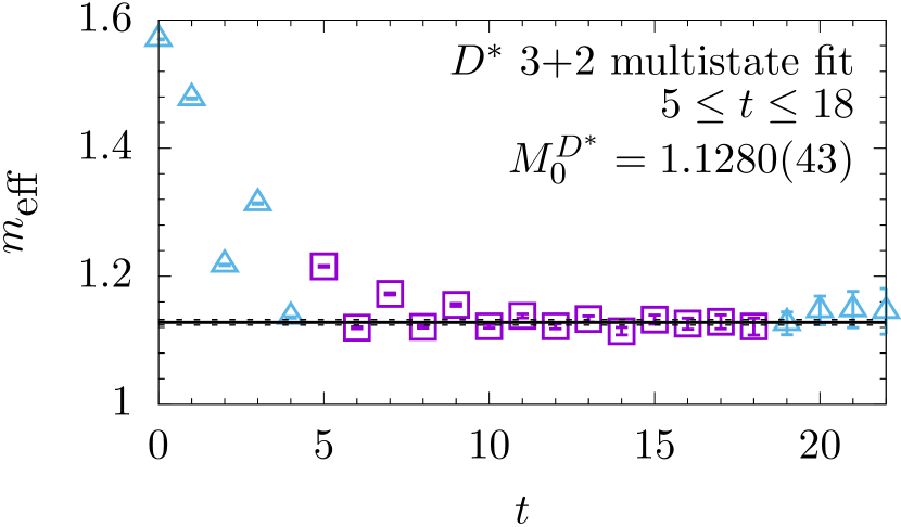
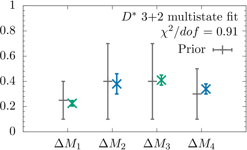
Figure 1: (Left) Effective mass, $m_{\text{eff}}(t)\equiv\frac{1}{2}\ln|C^{2pt}(t)/C^{2pt}(t+2)|$, plot using the 3+2-state fit to the 2pt function on the a12m310 ensemble for the $D^{\ast}$-meson with $m_{x}/m_{s}=0.2$. The ground state mass is shown as a horizontal line. (Right) The excited state masses from the 3+2-states fit using empirical Bayesian priors.

The 3pt data is fit including $2+1$ states for $|B_{m}\rangle$ and $|D^{\ast}_{n}\rangle$ in the spectral decomposition:

$$C^{B\rightarrow D^{\ast}}_{A_{j}}(t,\tau)=\langle O_{D^{\ast}}^{\dagger}(0)A_{j}^{cb}(t)O_{B}(\tau)\rangle\qquad(0<t<\tau)$$ (3)

$$={\mathcal{A}^{D^{\ast}}_{0}\mathcal{A}^{B}_{0}}{\langle D^{\ast}_{0}|A^{cb}_{j}|B_{0}\rangle}e^{-{M_{B_{0}}}(\tau-t)}e^{-{M_{D^{\ast}_{0}}}t}-{\mathcal{A}^{D^{\ast}}_{0}\mathcal{A}^{B}_{1}}{\langle D^{\ast}_{0}|A^{cb}_{j}|B_{1}\rangle}(-1)^{\tau-t}e^{-{M_{B_{1}}}(\tau-t)}e^{-{M_{D^{\ast}_{0}}}t}$$

$$\quad-{\mathcal{A}^{D^{\ast}}_{1}\mathcal{A}^{B}_{0}}{\langle D^{\ast}_{1}|A^{cb}_{j}|B_{0}\rangle}(-1)^{t}e^{-{M_{B_{0}}}(\tau-t)}e^{-{M_{D^{\ast}_{1}}}t}+{\mathcal{A}^{D^{\ast}}_{1}\mathcal{A}^{B}_{1}}{\langle D^{\ast}_{1}|A^{cb}_{j}|B_{1}\rangle}(-1)^{\tau}e^{-{M_{B_{1}}}(\tau-t)}e^{-{M_{D^{\ast}_{1}}}t}$$

$$\quad+{\mathcal{A}^{D^{\ast}}_{2}\mathcal{A}^{B}_{0}}{\langle D^{\ast}_{2}|A^{cb}_{j}|B_{0}\rangle}e^{-{M_{B_{0}}}(\tau-t)}e^{-{M_{D^{\ast}_{2}}}t}+{\mathcal{A}^{D^{\ast}}_{0}\mathcal{A}^{B}_{2}}{\langle D^{\ast}_{0}|A^{cb}_{j}|B_{2}\rangle}e^{-{M_{B_{2}}}(\tau-t)}e^{-{M_{D^{\ast}_{0}}}t}$$

$$\quad-{\mathcal{A}^{D^{\ast}}_{2}\mathcal{A}^{B}_{1}}{\langle D^{\ast}_{2}|A^{cb}_{j}|B_{1}\rangle}(-1)^{\tau-t}e^{-{M_{B_{1}}}(\tau-t)}e^{-{M_{D^{\ast}_{2}}}t}-{\mathcal{A}^{D^{\ast}}_{1}\mathcal{A}^{B}_{2}}{\langle D^{\ast}_{1}|A^{cb}_{j}|B_{2}\rangle}(-1)^{t}e^{-{M_{B_{2}}}(\tau-t)}e^{-{M_{D^{\ast}_{1}}}t}$$

$$\quad+{\mathcal{A}^{D^{\ast}}_{2}\mathcal{A}^{B}_{2}}{\langle D^{\ast}_{2}|A^{cb}_{j}|B_{2}\rangle}e^{-{M_{B_{2}}}(\tau-t)}e^{-{M_{D^{\ast}_{2}}}t}+\cdots,$$ (4)

where $A_{j}^{cb}$ is the improved axial current inserted at time $t$, and $\mathcal{A}^{B}_{n}$, $\mathcal{A}^{D^{\ast}}_{m}$, $M_{D^{\ast}_{n}}$ and $M_{B_{m}}$ values are taken from fits to the 2pt functions. Similar fit functions are used for the other channels: $C^{D^{\ast}\rightarrow B}_{A_{1}}(t,\tau)$, $C^{B\rightarrow B}_{V_{4}}(t,\tau)$ and $C^{D^{\ast}\rightarrow D^{\ast}}_{V_{4}}(t,\tau)$. In all the fits, we skip four points next to the source and the sink that have the largest ESC. In Fig. 2, we display the ratio, $\mathcal{G}$,

$$\mathcal{G}(t,\tau) \equiv\frac{C^{B\to{D^{\ast}}}_{A_{j}}(t,\tau)}{\mathcal{A}^{D^{\ast}}_{0}\mathcal{A}^{B}_{0}e^{-M_{B_{0}}(\tau-t)}e^{-M_{D^{\ast}_{0}}t}}=\langle{D^{\ast}_{0}}|A_{j}^{cb}|B_{0}\rangle+\cdots,$$ (5)

where $\mathcal{A}^{B}_{0}$, $\mathcal{A}^{D^{\ast}}_{0}$, $M_{D^{\ast}_{0}}$ and $M_{B_{0}}$ are ground-state amplitudes and masses determined from 2pt function fits. $\mathcal{G}$ asymptotes to the ground state matrix element in the $t\to\infty$ and $\tau-t\to\infty$ limits. The data show the size of the ESC and the oscillatory nature of the convergence. The $(-1)^{\tau}{\langle D^{\ast}_{1}|A^{cb}_{j}|B_{1}\rangle}$ term controls the even-odd oscillation about the grey band while ${\langle D^{\ast}_{2}|A^{cb}_{j}|B_{2}\rangle}$ controls the convergence as $\tau\to\infty$ for both even or odd $\tau$ data. We also find that the contribution of terms of the form $(-1)^{\tau-t}{\langle D^{\ast}_{0}|A^{cb}_{j}|B_{1}\rangle}$ is tiny and that of $(-1)^{\tau-t}{\langle D^{\ast}_{1}|A^{cb}_{j}|B_{2}\rangle}$ is negligible. The latter is therefore set to zero in the final fits. On the other hand, the grey horizontal band in Fig. 2 is the ground-state matrix element obtained by fitting $C^{B\to{D^{\ast}}}_{A_{j}}(t,\tau)$ using Eq. (4), to which $\mathcal{G}$ should converge. These results from the fits are summarized in Table 2. Note that there is no significant improvement at ${\cal O}(\lambda)$ in $\langle B|V_{4}|B\rangle$ and $\langle D^{\ast}|V_{4}|D^{\ast}\rangle$, but a large change at ${\cal O}(\lambda^{2})$  (also see Fig. 4). Thus, higher order improvements for these two channels may be necessary.

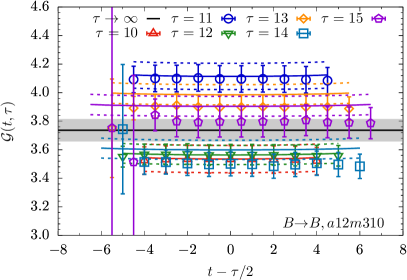
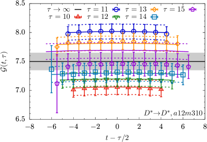
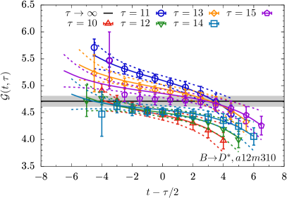
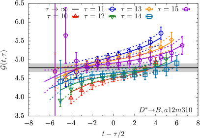
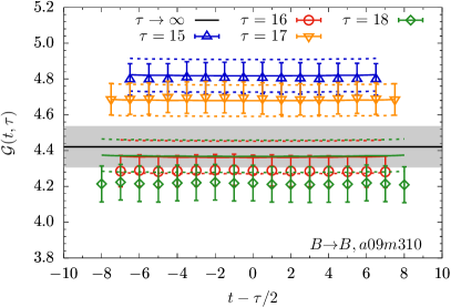
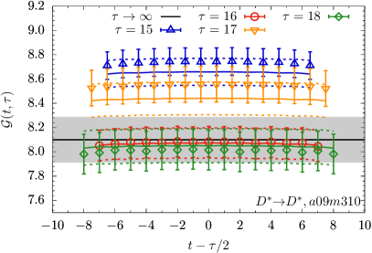
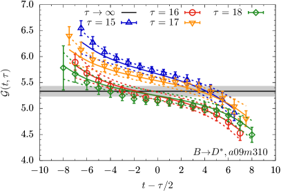
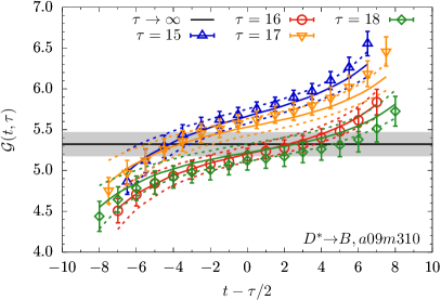
Figure 2: Data for the ratio $\mathcal{G}$ for the various values of $\tau$ (see labels) are plotted versus $t-\tau/2$ for the ${\cal O}(\lambda^{2})$ improved current and $m_{x}=0.2m_{s}$. The horizontal line is the ground-state matrix element ($\tau\to\infty$) determined from the multistate fit using Eq. (4). The results of the fit for each $\tau$ is shown in the same color as the data. Note the difference in ESC for $D^{\ast}\rightarrow B$ (or the rough mirror process $B\rightarrow D^{\ast}$) and $D^{\ast}\rightarrow D^{\ast}$ (or $B\rightarrow B$) and the change with $a$ between $a12m310$ (top 4 panels) and $a09m310$ (bottom 4 panels).

Current	$\langle B|V_{4}|B\rangle$	$\chi^{2}/\text{dof}\;[p]$	$\langle D^{\ast}|V_{4}|D^{\ast}\rangle$	$\chi^{2}/\text{dof}\;[p]$	$\langle D^{\ast}|A_{j}|B\rangle$	$\chi^{2}/\text{dof}\;[p]$	$\langle B|A_{j}|D^{\ast}\rangle$	$\chi^{2}/\text{dof}\;[p]$
Unimp.	3.88(8)	1.20 [0.21]	8.44(17)	0.73 [0.84]	4.79(10)	0.73 [0.84]	4.84(11)	0.89 [0.63]
${\cal O}(\lambda)$	3.89(8)	1.20 [0.21]	8.45(17)	0.73 [0.84]	4.90(10)	0.74 [0.83]	4.96(12)	0.84 [0.70]
${\cal O}(\lambda^{2})$	3.74(8)	1.27 [0.15]	7.50(15)	0.86 [0.68]	4.71(10)	0.73 [0.84]	4.79(11)	0.93 [0.56]

(a) Results for the $a12m310$ ensemble with $m_{x}=0.2m_{s}$.

Current	$\langle B|V_{4}|B\rangle$	$\chi^{2}/\text{dof}\;[p]$	$\langle D^{\ast}|V_{4}|D^{\ast}\rangle$	$\chi^{2}/\text{dof}\;[p]$	$\langle D^{\ast}|A_{j}|B\rangle$	$\chi^{2}/\text{dof}\;[p]$	$\langle B|A_{j}|D^{\ast}\rangle$	$\chi^{2}/\text{dof}\;[p]$
Unimp.	4.64(12)	1.44 [0.05]	9.26(22)	0.90 [0.63]	5.49(10)	1.54 [0.03]	5.48(15)	0.68 [0.91]
${\cal O}(\lambda)$	4.65(12)	1.44 [0.05]	9.27(22)	0.90 [0.63]	5.60(10)	1.54 [0.03]	5.60(15)	0.67 [0.92]
${\cal O}(\lambda^{2})$	4.42(12)	1.34 [0.09]	8.10(19)	0.84 [0.73]	5.33(10)	1.62 [0.02]	5.32(15)	0.76 [0.83]

(b) Results for the $a09m310$ ensemble with $m_{x}=0.2m_{s}$.

Table 2: Matrix elements of ${\cal O}(\lambda^{\ell})$ (with $\ell\in 0,1,2$) improved currents extracted from $2+1$-state fits.

3 $|h_{A_{1}}(1)/\rho_{A_{j}}|$ result

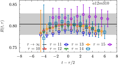
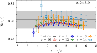
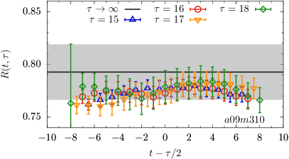
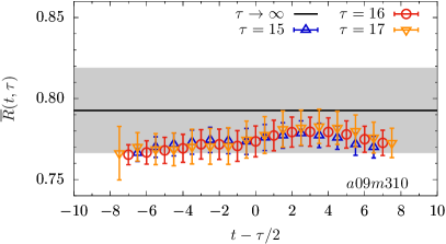
Figure 3: Data for the double ratio $R(t,\tau)$ for the various values of $\tau$ are plotted versus the operator insertion time $t-\tau/2$. The grey horizontal band is the result for $|h_{A_{1}}(1)/\rho_{A_{j}}|^{2}$ obtained using Eq. (1). The top (bottom) panels show data for the $a12m310$ ($a09m310$) ensemble at the unitary point $m_{x}=0.2m_{s}$. The left (right) panels show data for $R(t,\tau)$ ($\overline{R}(t,\tau)$) that are defined in the text.

We obtain $|h_{A_{1}}(1)/\rho_{A_{j}}|^{2}$, defined in Eq. (1), using the ground-state matrix elements given in Table 2. The result for the two values of the lattice spacing at fixed pion mass $M_{\pi}\approx 310$ MeV (unitary point) is shown by the grey horizontal band in all panels of Fig. 3. The error estimate includes the uncertainty coming from the fits used to remove excited-state effects. The left two panels in Fig. 3 show the data for the double ratio $R(t,\tau)$

$$R(t,\tau)=\frac{C^{B\rightarrow D^{\ast}}_{A_{1}}(t,\tau)C^{D^{\ast}\rightarrow B}_{A_{1}}(t,\tau)}{C^{B\rightarrow B}_{V_{4}}(t,\tau)C^{D^{\ast}\rightarrow D^{\ast}}_{V_{4}}(t,\tau)},$$ (6)

that significantly cancels the ESC in each individual correlator illustrated in Fig. 2. The right panels in Fig. 3 show the linear combination $\overline{R}(t,\tau)$ defined as [5],

$$\overline{R}(t,\tau)=\frac{1}{2}R(t,\tau)+\frac{1}{4}R(t,\tau+1)+\frac{1}{4}R(t+1,\tau+1)\,,$$ (7)

that further suppresses the ESC, especially from the opposite parity states. Since the grey band in Fig. 3 is constructed as the ratio of ground state matrix elements (albeit evaluated using 2+1 state fits), both the ratios, $R(t,\tau)$ and $\overline{R}(t,\tau)$ should asymptote to it in the $t\to\infty$ and $(\tau-t)\to\infty$ limits. We find that $R(t,\tau)$ and $\overline{R}(t,\tau)$ overlap with the grey band, however the spread due to remaining ESC is larger in $R(t,\tau)$ than in $\overline{R}(t,\tau)$. In fact, on the finer $a09m310$ ensemble, we do not observe a spread in $\overline{R}(t,\tau)$ versus $\tau$, however, the comparison with the grey band suggests that quoting the average of the $\overline{R}(t,\tau)$ data as the final result could underestimate the error.

The data for $|h_{A_{1}}(1)/\rho_{A_{j}}|$ in Fig. 4 (left) show no significant dependence on the spectator quark mass $m_{x}$. The observed dependence on the order of improvement in the current is unexpected from naive HQET power counting and could an artifact of setting $\rho_{A_{j}}=1$, which also depends on the order of improvement. In Fig. 4 (right), we compare our results with those from the FNAL/MILC and HPQCD collaborations [5, 11] obtained in the continuum limit. The $O(\lambda^{2})$ data are consistent with the FNAL/MILC and HPQCD results and show no significant lattice spacing dependence. This rough agreement provides a good and encouraging check of our calculations that are being done with a much more complicated heavy quark action and current.

A brief summary of the work under progress is as follows. (i) Analysis with the ${\cal O}(\lambda^{3})$-improvement terms in the current, (ii) analysis of the data for the nonzero recoil form factors in $B\to D^{(\ast)}\ell\nu$ decays, and (iii) the analysis for the decay constants $f_{D}$, $f_{D_{s}}$, $f_{B}$, $f_{B_{s}}$ and $f_{B_{c}}$.

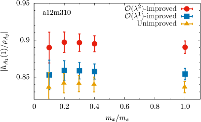
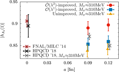
Figure 4: (Left) Data for $|h_{A_{1}}(1)/\rho_{A_{1}}|$ for three levels of current improvement plotted versus the spectator quark mass $m_{x}$ for the $a12m310$ ensemble. (Right) Comparison of data on two different ensembles, $a12m310$ and $a09m310$ at the unitary point $m_{x}=0.2m_{s}$, and with $\rho_{A_{1}}=1$ to investigate $a$ dependence, and to compare with FNAL/MILC and HPQCD collaboration results [5, 11] obtained in the continuum limit.

- [1] Y. Amhis et al. Eur. Phys. J. C77 (2017), no. 12 895, [1612.07233].
- [2] J. A. Bailey, S. Lee, W. Lee, J. Leem, and S. Park 1808.09657.
- [3] M. B. Oktay and A. S. Kronfeld Phys. Rev. D78 (2008) 014504, [0803.0523].
- [4] J. A. Bailey, C. DeTar, Y.-C. Jang, A. S. Kronfeld, W. Lee, and M. B. Oktay Eur. Phys. J. C77 (2017), no. 11 768, [1701.00345].
- [5] J. A. Bailey et al. Phys. Rev. D89 (2014), no. 11 114504, [1403.0635].
- [6] A. X. El-Khadra, A. S. Kronfeld, and P. B. Mackenzie Phys. Rev. D55 (1997) 3933–3957, [hep-lat/9604004].
- [7] J. Bailey, Y.-C. Jang, W. Lee, and J. Leem EPJ Web Conf. 175 (2018) 14010, [1711.01777].
- [8] J. A. Bailey, T. Bhattacharya, R. Gupta, Y.-C. Jang, W. Lee, J. Leem, S. Park, and B. Yoon EPJ Web Conf. 175 (2018) 13012, [1711.01786].
- [9] A. Bazavov et al. Phys. Rev. D87 (2013), no. 5 054505, [1212.4768].
- [10] B. Yoon et al. Phys. Rev. D95 (2017), no. 7 074508, [1611.07452].
- [11] J. Harrison, C. Davies, and M. Wingate Phys. Rev. D97 (2018), no. 5 054502, [1711.11013].