G. Celeux, K. Kamary, G. Malsiner-Walli, J.-M. Marin, and C. P. Robert

Computational Solutions for Bayesian Inference in Mixture Models

This chapter surveys the most standard Monte Carlo methods available for simulating from a posterior distribution associated with a mixture and conducts some experiments about the robustness of the Gibbs sampler in high dimensional Gaussian settings.

1 Introduction

It may sound paradoxical that a statistical model that writes as a sum of Gaussian densities poses a significant computational challenge to Bayesian (and non-Bayesian alike) statisticians, but it is nonetheless the case. Estimating (and more globally running a Bayesian analysis on) the parameters of a mixture model has long been deemed impossible, except for the most basic cases, as illustrated by the approximations found in the literature of the 1980’s (Smith and Makov, 1978; Titterington et al., 1985; Bernardo and Girón, 1988; Crawford et al., 1992). Before the introduction of Markov chain Monte Carlo (MCMC) methods to the Bayesian community, there was no satisfying way to bypass this problem and it is no surprise that mixture models were among the first applications of Gibbs sampling to appear (Diebolt and Robert, 1990b; Gelman and King, 1990; West, 1992). The reason for this computational challenge is the combinatoric explosive nature of the development of the likelihood function, which contains $G^{n}$ terms when using $G$ components over $n$ observations. As detailed in other chapters, like Chapter 1, the natural interpretation of the likelihood is to contemplate all possible partitions of the $n$-observation sample $\mathbf{y}=(y_{1},\ldots,y_{n}$). While the likelihood function can be computed in $\mathcal{O}(G\times n)$ time, being expressed as

$$p(\mathbf{y}|\theta)=\prod_{i=1}^{n}\sum_{g=1}^{G}\eta_{g}f(y_{i}|\theta_{g})\,,$$

where $\theta=(\theta_{1},\ldots,\theta_{G},\eta_{1},\ldots,\eta_{G})$, there is no structure in this function that allows for its exploration in an efficient way. Indeed, as demonstrated for instance by Chapter 2, the variations of this function are not readily available and require completion steps as in the EM algorithm. Given a specific value of $\theta$, one can compute $p(\mathbf{y}|\theta)$ but this numerical value does not bring useful information on the shape of the likelihood in a neighbourhood of $\theta$. The value of the gradient also is available in $\mathcal{O}(G\times n)$ time, but does not help much in this regard. (Several formulations of the Fisher information matrix for, e.g., Gaussian mixtures through special functions are available, see, e.g., Behboodian, 1972 and Cappé et al., 2004.)

Computational advances have thus been essential to Bayesian inference on mixtures while this problem has retrospectively fed new advances in Bayesian computational methodology. In Section 2 we cover some of the proposed solutions, from the original Data Augmentation of Tanner and Wong (1987) that predated the Gibbs sampler of Gelman and King (1990) and Diebolt and Robert (1990b) to specially designed algorithms, to the subtleties of label switching (Stephens, 2000).

As stressed by simulation experiments in Section 4, there nonetheless remain major difficulties in running Bayesian inference on mixtures of moderate to large dimensions. First of all, among all the algorithms that will be reviewed only Gibbs sampling seems to scale to high dimensions. Second, the impact of the prior distribution remains noticeable for sample sizes that would seem high enough in most settings, while larger sample sizes see the occurrence of extremely peaked posterior distributions that are a massive challenge for exploratory algorithms like MCMC methods. Section 5 is specifically devoted to Gibbs sampling for high-dimensional Gaussian mixtures and a new prior distribution is introduced that seems to scale appropriately to high dimensions.

2 Algorithms for Posterior Sampling

2.1 A computational problem? Which computational problem?

When considering a mixture model from a Bayesian perspective (see, e.g., Chapter 4), the associated posterior distribution

$$p(\theta|\mathbf{y})\propto p(\theta)\prod_{i=1}^{n}\sum_{g=1}^{G}\eta_{g}f(y_{i}|\theta_{g}),$$

based on the prior distribution $p(\theta)$, is available in closed form, up to the normalising constant, because the number of terms to compute is of order $\mathcal{O}(G\times n)$ in dimension one and of order $\mathcal{O}(G\times n\times d^{2})$ in dimension $d$. This means that two different values of the parameter can be compared through their (non-normalized) posterior values. See for instance Figure 1 that displays the posterior density surface in the case of the univariate Gaussian mixture

$$\frac{3}{10}\,\mathcal{N}(\mu_{1},1)+\frac{7}{10}\,\mathcal{N}(\mu_{2},1)\,,$$

clearly identifying a modal region near the true value of the parameter $(\mu_{1},\mu_{2})=\left(0,\frac{5}{2}\right)$ actually used to simulate the data. However, this does not mean a probabilistic interpretation of $p(\theta|\mathbf{y})$ is immediately manageable: deriving posterior means, posterior variances, or simply identifying regions of high posterior density value remains a major difficulty when considering only this function. Since the dimension of the parameter space grows quite rapidly with $G$ and $d$, being for instance $3G-1$ for a unidimensional Gaussian mixture against $G-1+dG+(d(d+1)/2)G$ for a $d$-dimensional Gaussian mixture, numerical integration cannot be considered as a viable alternative. Laplace approximations (see, e.g., Rue et al., 2009) are incompatible with the multimodal nature of the posterior distribution. The only practical solution thus consists of producing a simulation technique that approximates outcomes from the posterior. In principle, since the posterior density can be computed up to a constant, MCMC algorithms should operate smoothly in this setting. As we will see in this chapter, this is not always the case.

Figure 1: Posterior density surface for $100$ observations from the Gaussian mixture $\nicefrac{{3}}{{10}}\mathcal{N}(\mu_{1},1)+\nicefrac{{7}}{{10}}\mathcal{N}(\mu_{2},1)$, clearly identifying a modal region near the true value of the parameter $(\mu_{1},\mu_{2})=(0,\nicefrac{{5}}{{2}})$ used to simulate the data, plus a secondary mode associated with the inversion of the data allocation to the two components. The figure was produced by computing the likelihood and prior functions over a $100\times 100$ grid over $(-1,3)\times(-1,3)$. The level sets in the image are expressed in a logarithmic scale.

2.2 Gibbs sampling

Prior to 1989 or more exactly to the publication by Tanner and Wong (1987) of their Data Augmentation paper, which can be considered as a precursor to the Gelfand and Smith 1990 Gibbs sampling paper, there was no manageable way to handle mixtures from a Bayesian perspective. As an illustration on an univariate Gaussian mixture with two components, Diebolt and Robert (1990a) studied a “grey code”  implementation for exploring the collection of all partitions of a sample of size $n$ into $2$ groups and managed to reach $n=30$ within a week of computation (in 1990’s standards).

Consider thus a mixture of $G$ components

$$\sum_{g=1}^{G}\;\eta_{g}\;f(y|\theta_{g})\;,\qquad y\in\mathbb{R}^{d}\,,$$ (1)

where, for simplicity’s sake, $f(\cdot|\theta)$ belongs to an exponential family

$$f(y|\theta)=h(y)\;\exp\{\theta\cdot y-\psi(\theta)\}$$

over the set $\mathbb{R}^{d}\,,$ and where $(\theta_{1},\ldots,\theta_{G})$ is distributed from a product of conjugate priors

$$p(\theta_{g}|\alpha_{g},\lambda_{g})\propto\exp\{\lambda_{g}(\theta_{g}\cdot\alpha_{g}-\psi(\theta_{g}))\}\;,$$

with hyperparameters $\lambda_{g}>0$ and $\alpha_{g}\in\mathbb{R}^{d}$ $(g=1,\ldots,G)$, while $(\eta_{1},\ldots,\eta_{G})$ follows the usual Dirichlet prior:

$$(\eta_{1},\ldots,\eta_{G})\sim\mathcal{D}(e_{1},\ldots,e_{G})\;.$$

These prior choices are only made for convenience sake, with hyperparameters requiring inputs from the modeller. Most obviously, alternative priors can be proposed, with a mere increase in computational complexity. Given a sample $(y_{1},\ldots,y_{n})$ from (1), then as already explained in Chapter 1, we can associate to every observation an indicator random variable $z_{i}\in\{1,\ldots,G\}$ that indicates which component of the mixture is associated with $y_{i}$, namely which term in the mixture was used to generate $y_{i}$. The demarginalization (or completion) of model (1) is then

$$z_{i}\sim\mbox{\rm MulNom}(1,\eta_{1},\ldots,\eta_{G}),\qquad y_{i}|z_{i}\sim f(y_{i}|\theta_{z_{i}})\;.$$

Thus, considering $x_{i}=(y_{i},z_{i})$ (instead of $y_{i}$) entirely eliminates the mixture structure from the model since the likelihood of the completed model (the so-called complete-data likelihood function) is given by:

$${\text{L}}_{\text{c}}(\theta|x_{1},\ldots,x_{n}) \propto \prod_{i=1}^{n}\;\eta_{z_{i}}\;f(y_{i}|\theta_{z_{i}})$$

$$= \prod_{g=1}^{G}\;\prod_{i;z_{i}=g}\;\eta_{g}\;f(y_{i}|\theta_{g})\;.$$

Algorithm 1 Mixture Posterior Simulation

Set hyperparameters $(\alpha_{g},e_{g},\lambda_{g})_{g}$. Repeat the following steps $T$ times, after a suitable burn-in phase:

0:   Simulate $z_{i}\;\;(i=1,\ldots,n)$ from

$$\mbox{\rm P}(z_{i}=g|\theta_{g},\eta_{g},y_{i})\propto\eta_{g}\;f(y_{i}|\theta_{g}),\qquad(g=1,\ldots,G),$$

and compute the statistics

$$n_{g}=\sum_{i=1}^{n}\;\mathbb{I}(z_{i}=g)\;,\qquad n_{g}{\overline{y}}_{g}=\sum_{i=1}^{n}\;\mathbb{I}(z_{i}=g)y_{i}\;.$$

0:   Generate $(g=1,\ldots,G)$

$$\theta_{g}|\mathbf{z},\mathbf{y}\sim\displaystyle{p\left(\theta_{g}\bigg{|}{\lambda_{g}\alpha_{g}+n_{g}{\overline{y}}_{g}\over\lambda_{g}+n_{g}},\lambda_{g}+n_{g}\right)}\,,$$

$$(\eta_{1},\ldots,\eta_{G})|\mathbf{z},\mathbf{y}\sim\mathcal{D}_{G}(e_{1}+n_{1},\ldots,e_{G}+n_{G})\;.$$

This latent structure is also exploited in the original implementation of the EM algorithm, as discussed in Chapter 2. Both steps of the Gibbs sampler (Robert and Casella, 2004) are then provided in Algorithm 1, with a straightforward simulation of all components indices in parallel in Step 1 and a simulation of the parameters of the mixture exploiting the conjugate nature of the prior against the complete-data likelihood function in Step 2. Some implementations of this algorithm for various distributions from the exponential family can be found in the reference book of Frühwirth-Schnatter (2006).

Illustration

As an illustration, consider the setting of a univariate Gaussian mixture with two components with equal and known variance $\sigma^{2}$ and fixed weights $(\eta,1-\eta)$:

$$\eta\,\mathcal{N}(\mu_{1},\sigma^{2})+(1-\eta)\,\mathcal{N}(\mu_{2},\sigma^{2})\,.$$ (2)

The only parameters of the model are thus $\mu_{1}$ and $\mu_{2}$. We assume in addition a Normal $\mathcal{N}(0,10\sigma^{2})$ prior distribution on both means $\mu_{1}$ and $\mu_{2}$. Generating directly i.i.d. samples of $(\mu_{1},\mu_{2})$’s distributed according to the posterior distribution associated with an observed sample $\mathbf{y}=(y_{1},\ldots,y_{n})$ from (2) quickly become impossible, as discussed for instance in Diebolt and Robert (1994) and Celeux et al. (2000), because of a combinatoric explosion in the number of calculations, which grow as $\mathcal{O}(2^{n})$. The posterior is indeed solely interpretable as a well-defined mixture of standard distributions that involves that number of components.

As explained above, a natural completion of $(\mu_{1},\mu_{2})$ is to introduce the (unobserved) component indicators $z_{i}$ of the observations $y_{i}$, in a similar way as for the EM algorithm, namely,

$$\mbox{\rm P}(z_{i}=1)=1-\mbox{\rm P}(z_{i}=2)=\eta\qquad\mbox{and}\qquad y_{i}|z_{i}=g\sim\mathcal{N}(\mu_{g},\sigma^{2})\,.$$

The completed distribution with $\mathbf{z}=(z_{1},\ldots,z_{n})$ is thus

$$p(\mu_{1},\mu_{2},\mathbf{z}|\mathbf{y}) \propto\exp\{-(\mu_{1}^{2}+\mu_{2}^{2})/20\sigma^{2}\}\,\prod_{i;z_{i}=1}\eta\exp\{-(y_{i}-\mu_{1})^{2}/2\sigma^{2}\}\,\times$$

$$\prod_{i;z_{i}=2}(1-\eta)\exp\{-(y_{i}-\mu_{2})^{2}/2\sigma^{2}\}\,.$$

Since $\mu_{1}$ and $\mu_{2}$ are independent, given $(\mathbf{z},\mathbf{y})$, the conditional distributions are $(g=1,2)$:

$$\mu_{g}|\mathbf{y}\sim\mathcal{N}\left(\sum_{i;z_{i}=g}y_{i}/\left(0.1+n_{g}\right),\sigma^{2}/\left(0.1+n_{g}\right)\right)\,,$$

where $n_{g}$ denotes the number of $z_{i}$’s equal to $g$ and 0.1=1/10 represent the prior precision. Similarly, the conditional distribution of $\mathbf{z}$ given $(\mu_{1},\mu_{2})$ is a product of binomials, with

$$\mbox{\rm P}(z_{i}=1|y_{i},\mu_{1},\mu_{2})$$

$$= \frac{\eta\exp\{-(y_{i}-\mu_{1})^{2}/2\sigma^{2}\}}{\eta\exp\{-(y_{i}-\mu_{1})^{2}/2\sigma^{2}\}+(1-\eta)\exp\{-(y_{i}-\mu_{2})^{2}/2\sigma^{2}\}}\,.$$

Figure 2 illustrates the behavior of the Gibbs sampler in that setting, with a simulated data set of $5,000$ points from the $0.7\mathcal{N}(0,1)+0.3\mathcal{N}(2.5,1)$ distribution. The representation of the MCMC sample after $15,000$ iterations is quite in agreement with the posterior surface, represented via a grid on the $(\mu_{1},\mu_{2})$ space and some contours; while it may appear to be too concentrated around one mode, the second mode represented on this graph is much lower since there is a difference of at least $50$ in log-posterior units.

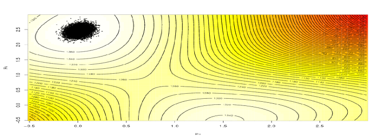
Figure 2: Gibbs sample of $5,000$ points for the mixture posterior against the posterior surface. The level sets in the image are expressed in a logarithmic scale. (Reproduced with permission from Robert and Casella, 2004.)

However, the Gibbs sampler may also fail to converge, as described in Diebolt and Robert (1994) and illustrated in Figure 3. When initialised at the secondary mode of the likelihood, the magnitude of the moves around this mode may be too limited to allow for exploration of further modes (in a realistic number of iterations).

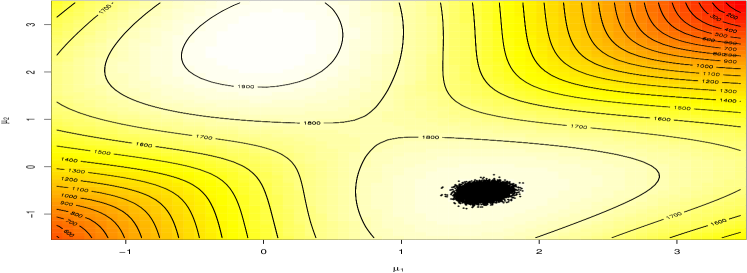
Figure 3: Gibbs sample for the two mean mixture model, when initialised close to the second and lower mode, for true values $\mu_{1}=0$ and $\mu_{2}=2.5$, over the log-likelihood surface. (Reproduced with permission from Robert and Casella, 2004.)

Label switching

Unsurprisingly, given the strong entropy of the local modes demonstrated in the illustrative example, Gibbs sampling performs very poorly in terms of label switching (already discussed in Chapter 1) in that it rarely switches between equivalent modes of the posterior distribution. One (if not the only) reason for this behaviour is that, due to the allocation of the observations to the various components, i.e., by completing the unknown parameters with the unknown (and possibly artificial) latent variables, the Gibbs sampler faces enormous difficulties in switching between equivalent modes, because this amounts to changing the values of most latent variables to a permuted version all at once. It can actually be shown that the probability of seeing a switch goes down to zero as the sample size $n$ goes to infinity. This difficulty is increasing with dimension, in the sense that the likelihood function increasingly peaks with the dimension.

Some (as, e.g., Geweke, 2007) would argue the Gibbs sampler does very well by naturally selecting a mode and sticking to it. This certainly favours estimating the parameters of the different components. However, there is no guarantee that the Gibbs sampler will remain in the same mode over iterations.

The problem can alleviated to a certain degree by enhancing the Gibbs sampler (or any other simulation based technique) to switch between equivalent modes. A simple, but efficient, solution to obtain a sampler that explores all symmetric modes of the posterior distribution is to enforce balanced label switching by concluding each MCMC draw by a random permutation of the labels. Let $\mathfrak{S}(G)$ denote the set of the $G!$ permutations of $\{1,\ldots,G\}$. Assume that $(\eta_{1},\ldots,\eta_{G})$ follows the symmetric Dirichlet distribution $\mathcal{D}_{G}\left(e_{0}\right)$ (which corresponds to the $\mathcal{D}(e_{0},\ldots,e_{0})$ distribution and is invariant to permuting the labels by definition) and assume that also the prior on $\theta_{g}$ is invariant in this respect, i.e. $p(\theta_{\mathfrak{s}(1)},\ldots,\theta_{\mathfrak{s}(G)})=p(\theta_{1},\ldots,\theta_{G})$ for all permutations $\mathfrak{s}\in\mathfrak{S}(G)$. Then, for any given posterior draw $\theta=(\eta_{1},\ldots,\eta_{G},\theta_{1},\ldots,\theta_{G})$, jumping between the equivalent modes of the posterior distribution can be achieved by defining the permuted draw $\mathfrak{s}(\theta):=(\eta_{\mathfrak{s}(1)},\ldots,\eta_{\mathfrak{s}(G)},\theta_{\mathfrak{s}(1)},\ldots,\theta_{\mathfrak{s}(G)})$ for some permutation $\mathfrak{s}\in\mathfrak{S}(G)$.

This idea underlies the random permutation sampler introduced by Frühwirth-Schnatter (2001), where each of the $T$ sweeps of Algorithm 1 is concluded by such a permutation of the labels, based on randomly selecting one of the $G!$ permutations $\mathfrak{s}\in\mathfrak{S}(G)$, see also Frühwirth-Schnatter (2006, Section 3.5.6). Admittedly, this method works well only, if $G!\ll T$, as the expected number of draws from each modal region is equal to $T/G!$. Geweke (2007) suggests to consider all of the $G!$ permutations in $\mathfrak{S}(G)$ for each of the $T$ posterior draw, leading to a completely balanced sample of $T\times G!$ draws, however the resulting sample size can be enormous, if $G$ is large.

As argued in Chapter 1, the difficulty in exploring all modes of the posterior distribution in the parameter space is not a primary concern provided the space of mixture distributions (that are impervious to label-switching) is correctly explored. Since this is a space that is much more complex than the Euclidean parameter space, checking proper convergence is an issue. Once again, this difficulty is more acute in larger dimensions and it is compounded by the fact that secondary modes of the posterior become so “sticky”  that a standard Gibbs sampler cannot escape their (fatal) attraction. It may therefore be reasonably argued, as in Celeux et al. (2000) that off-the-shelf Gibbs sampling does not necessarily work for mixture estimation, which would not be an issue in itself were alternative generic solutions readily available!

Label switching, however, still matters very much when considering the statistical evidence (or marginal likelihood) associated with a particular mixture model, see also Chapter 7. This evidence can be easily derived from Bayes’ theorem by Chib’s (1995) method, which can also be reinterpreted as a Dickey-Savage representation (Dickey, 1968), except that the Rao-Blackwell representation of the posterior distribution of the parameters is highly dependent on a proper mixing over the modes. As detailed in Neal (1999) and expanded in Frühwirth-Schnatter (2004), a perfect symmetry must be imposed on the posterior sample for the method to be numerically correct. In the most usual setting when this perfect symmetry fails, it must be imposed in the estimate, as proposed in Berkhof et al. (2003) and Lee and Robert (2016), see also Chapter 7 for more details.

2.3 Metropolis–Hastings schemes

As detailed at the beginning of this chapter, computing the likelihood function at a given parameter value $\theta$ is not a computational challenge provided (i) the component densities are available in closed-form and (ii) the sample size remains manageable, e.g., fits within a single computer memory. This property means that an arbitrary proposal can be used to devise a Metropolis–Hastings algorithm (Robert and Casella, 2004; Lee et al., 2008) associated with a mixture model, from a simple random walk to more elaborate solutions like Langevin and Hamiltonian Monte Carlo.

The difficulty with this Metropolis–Hastings approach is to figure out an efficient way of implementing the simulating principle, which does not provide guidance on the choice of the proposal distribution. Parameters are set in different spaces, from the $G$-dimensional simplex of $\mathbb{R}^{G}$ to real vector spaces. A random walk is thus delicate to calibrate in such a context and it is often preferable to settle for a Gibbs sampler that updates one group of parameters at a time, for instance the weights, then the variances, then the means in the case of a location-scale mixture. This solution however shares some negative features with the original Gibbs sampler in the sense that it may prove a hardship to explore the entire parameter space (even without mentioning the label switching problem). Still, the implementation of the unidimensional location-parameterisation of Kamary et al. (2018) relies on this block-wise version and manages to handle a reasonably large number of components, if not a larger number of dimensions. Indeed, when the dimension $d$ of the observables increases, manipulating $d\times d$ matrices gets particularly cumbersome and we know of no generic solution to devise an automatic random walk Metropolis–Hastings approach in this case.

Among the strategies proposed to increase the efficiency of a Metropolis–Hastings algorithm in dimension one, let us single out the following ones:

1. Deriving independent proposals based on sequential schemes starting for instance from maximum likelihood and other classical estimates, since those are usually fast to derive, and followed by mixture proposals based on subsamples, at least in low dimensional models;

2. An overparameterisation of the weights $\eta_{g}$ defined as $\eta_{g}=\alpha_{g}/\sum_{j}\alpha_{j}$, with a natural extension of the Dirichlet prior $\mathcal{D}(e_{0},\ldots,e_{0})$ into a product of $d$ Gamma priors on the $\alpha_{g}$’s, where $\alpha_{g}\sim\mathcal{G}(e_{0},1)$. This representation avoids restricted simulations over the simplex of $\mathbb{R}^{G}$ and adding an extra parameter means the corresponding Markov chain mixes better;

3. The inclusion of the original Gibbs steps between random exploration proposals, in order to thoroughly survey the neighbourhood of the current value. Gibbs sampling indeed shares to some extent the same property as the EM algorithm to shoot rapidly towards a local mode when started at random. In this respect, it eliminates the random walk poor behaviour of a standard Metropolis–Hastings algorithm. Cumulating this efficient if myopic exploration of the Gibbs sampler with the potential for mode jumping associated with the Metropolis–Hastings algorithm may produce the best of two worlds, in the sense that mixture proposals often achieve higher performances than both of their components (Tierney, 1994);

4. Other mixings of different types of proposals, using for instance reparameterisation, overparameterisation, or underparameterisation. One important example is given by Rousseau and Mengersen (2011). In this paper, already discussed in Chapters 1 and 4, the authors consider mixtures with “too many” components and demonstrate that a Bayesian analysis of such overfitted models manages to eliminate the superfluous components. While this is an asymptotic result and while it imposes some constraints on the choice of the prior distribution on the weights, it nonetheless produces a theoretical warranty that working with more components than needed is not ultimately damaging to inference, while allowing in most situations for a better mixing behaviour of the MCMC sampler;

5. Deriving nonparametric estimates based for instance on Dirichlet process mixtures returns a form of clustering that can be exploited to build component-wise proposal;

6. Approximate solutions like nested sampling (see below), variational Bayes (Zobay, 2014), or Expectation–Propagation (EP, Minka, 2001; Titterington, 2011) may lead to independent proposals that contribute to a larger degree of mobility over the posterior surface;

7. Further sequential, tempering, and reversible jump solutions as discussed below.

At this stage, while the above has exhibited a medley of potential fixes to the Metropolis–Hasting woes, it remains urgent to warn the reader that no generic implementation is to be found so far (in the sense of a generic software able to handle a wide enough array of cases). The calibration stage of those solutions remains a challenging issue that hinders and in some cases prevents an MCMC resolution of the computational problem. This is almost invariably the case when the dimension of the model gets into double digits, see Section 5.

2.4 Reversible jump MCMC

It may seem inappropriate to include a section or even a paragraph on reversible jump MCMC (Green, 1995) in this chapter since we are not directly concerned with estimating the number of components, however, this approach to variable or unknown $G$ environments is sometimes advanced as a possible mean to explore better the parameter space by creating passageways through spaces of larger (and possibly smaller) dimensions and numbers of component. As discussed in Chopin and Robert (2010), this strategy is similar to bridge sampling. Once again, calibration of the method remains a major endeavour (Richardson and Green, 1997), especially in multidimensional settings, and we thus abstain from describing this solution any further.

2.5 Sequential Monte Carlo

Sequential Monte Carlo methods (see Del Moral et al., 2006) approach posterior simulation by a sequence of approximations, each both closer to the distribution of interest and borrowing strength from the previous approximation. They therefore apply even in settings where the data is static and entirely available from the start. They also go under the names of particle systems and particle filters.

Without getting into a full description of the way particle systems operate, let us recall here that this is a particular type of iterated importance sampling where, at each iteration $t$ of the procedure, a weighted sample $(\theta_{1t},\ldots,\theta_{Nt})$ of size $N$ is produced, with weights $\omega_{it}$ targeting a distribution $\pi_{t}$. The temporal and temporary target $\pi_{t}$ may well be supported by another space than the support of the original target $\pi$. For instance, in Everitt et al. (2016), the $\pi_{t}$’s are the posterior distributions of mixtures with a lesser number of components, while in Chopin (2002) they are posterior distributions of mixtures with a lesser number of observations. The sample or particle system at time $t$ is instrumental in designing the importance proposal for iteration $t+1$, using for instance MCMC-like proposals for simulating new values. When the number of iterations is large enough and the temporary targets $\pi_{t}$ are too different, the importance weights necessarily deteriorate down to zero (by basic martingale theory) and particle systems include optional resampling steps to select particles at random based on the largest weights, along with a linear increase in the number of particles as $t$ grows. The construction of the sequence of temporary targets $\pi_{t}$ is open and intended to facilitate the exploration of intricate and highly variable distributions, although its calibration is delicate and may jeopardise convergence.

In the particular setting of Bayesian inference, and in the case of mixtures, a natural sequence can be associated with subsample posteriors, namely posteriors constructed with only a fraction of the original data, as proposed for instance in Chopin (2002, 2004). The starting target $\pi_{0}$ may for instance correspond to the true prior or to a posterior with a minimal sample size (Robert, 2007). A more generic solution is to replace the likelihood with small powers of the likelihood in order to flatten out the posterior and hence facilitate the exploration of the parameter space. A common version of the proposal is then to use a random walk, which can be calibrated in terms of the parameterisation of choice and of the scale based on the previous particle system. The rate of increase of the powers of the likelihood can also be calibrated in terms of the degeneracy rate in the importance weights. This setting is studied by Everitt et al. (2016) who point out the many connections with reversible jump MCMC.

2.6 Nested sampling

While nested sampling is a late-comer to the analysis of mixtures (Skilling, 2004), one of the first examples of using this evidence estimation technique is a mixture example. We cannot recall the basics and background of this technique here and simply remind the reader that it consists of simulating a sequence of particles over subsets of the form

$$\left\{\theta;{\text{L}}(\theta|\mathbf{y})\geq\alpha\right\}$$

where L is the likelihood function and $\alpha$ a bound updated at each iteration of the algorithm, by finding the lowest likelihood in the current sample and replacing the argument with a new value with a higher likelihood. For a mixture model this approach offers the advantage of using solely the numerical value of the likelihood at a given parameter value, rather than exploiting more advanced features of this function. The resulting drawback is that the method is myopic, resorting to the prior or other local approximations for proposals. As the number of components, hence the dimension of the parameter, increases, it becomes more and more difficult to find moves that lead to higher values of the likelihood. In addition, the multimodality of the target distribution implies that there are more and more parts of the space that are not explored by the method (Chopin and Robert, 2010; Marin and Robert, 2010). While dimension (of the mixture model as well as of the parameter space) is certainly an issue and presumably a curse (Buchner, 2014) the Multinest version of the algorithm manages dimensions up to 20 (Feroz et al., 2013), which remains a small number when considering multivariate mixtures.

3 Bayesian Inference in the Model-based Clustering Context

In addition to being a probabilistic model per se, finite mixture models provide a well-known probabilistic approach to clustering. In the model-based clustering setting each cluster is associated with a mixture component. Usually clustering is relevant and useful for data analysis when the number of observations is large, involving say several hundreds of observations, and so is the number of variables, with say several dozens of variables. Moreover, choosing the unknown number $G$ of mixture components corresponding to the data clusters is a sensitive and critical task in this settings. Thus efficient Bayesian inference for model-based clustering requires MCMC algorithms working well and automatically in large dimensions with potentially numerous observations, which themselves requires smart strategies to derive a relevant number of clusters, see Chapter 7 for a detailed discussion.

Malsiner-Walli et al. (2016) devoted considerable efforts to assess relevant Bayesian procedures in a model-based clustering context and we refer the reader to this paper for detailed coverage. In this section, we only summarise their inference strategy, which consists primarily of choosing relevant prior distributions. As an illustration, their approach is implemented in the following section in a realistic if specific case with fifty variables and a relatively large number of observations.

We recall that the goal of the approach is to cluster $n$ individuals made of $d$ quantitative variables. In Malsiner-Walli et al. (2016), each cluster is associated with a multivariate Gaussian distribution, resulting formally in a multivariate Gaussian mixture sample with $G$ components

$$\sum_{g=1}^{G}\eta_{g}\mathcal{N}_{d}\left(\mu_{g},\Sigma_{g}\right)\,,$$

where $G$ is typically unknown.

Choosing priors for the mixing proportions

Malsiner-Walli et al. (2016)’s strategy consists of starting the analysis with an overfitted mixture, that is, a mixture with a number of components $G$ most likely beyond the supposed (if unknown) number of relevant clusters. Assuming a symmetric Dirichlet prior $\mathcal{D}_{G}\left(e_{0}\right)$ on the mixing proportions, they argue, based upon asymptotic results established in Rousseau and Mengersen (2011) and as observed in Frühwirth-Schnatter (2011), that if $e_{0}<r/2$, $r$ being the dimension of the component-specific parameter $\theta_{g}$, then the posterior expectation of the mixing proportions converges to zero for superfluous components. But if $e_{0}>r/2$ then the posterior density handles overfitting by defining at least two identical components, each with non-negligible weights. Thus Malsiner-Walli et al. (2016) favor small values of $e_{0}$ to allow emptying of superfluous components. More precisely, they consider a hierarchical prior distribution, namely a symmetric Dirichlet prior $\mathcal{D}_{G}\left(e_{0}\right)$ on the component weight distribution $(\eta_{1},\ldots,\eta_{G})$ and a Gamma hyperprior for $e_{0}$:

$$\eta_{1},\ldots,\eta_{G}|e_{0}\sim\mathcal{D}_{G}\left(e_{0}\right),\qquad e_{0}\sim\mathcal{G}(a,aG).$$

Based on numerical experiments on simulated data, they recommend setting $a=10$. An alternative choice is fixing the hyperparameter $e_{0}$ to a given small value.

Choosing the priors for the component means and covariance matrices

Following Frühwirth-Schnatter (2011), Malsiner-Walli et al. (2016) recommend putting a shrinkage prior, namely the Normal Gamma prior on component means. This prior is designed to handle high-dimensional mixtures, where not all variables contribute to the clustering structure, but a number of irrelevant variables is expected to be present without knowing a priori which variables this could be. For any such variable $y_{il}$ in dimension $l$, the components means $\mu_{l1},\ldots,\mu_{lG}$ are pulled toward a common value $b_{0l}$, due to a local, dimension-specific shrinkage parameter $\lambda_{l}$. More specifically, the following hierarchical prior based on a multivariate Normal distribution for the component means $\mu_{g}$ is chosen:

$$\displaystyle\mu_{g}\sim\mathcal{N}_{d}(b_{0},B_{0}),\quad g=1,\ldots,G,$$

$$\displaystyle b_{0}\sim\mathcal{N}_{d}(m_{0},M_{0}),\quad B_{0}=\Lambda R_{0}\Lambda,\quad R_{0}=\mbox{\rm Diag}(R_{1}^{2},\ldots,R_{d}^{2}),$$

$$\displaystyle\Lambda=\mbox{\rm Diag}(\sqrt{\lambda_{1}},\ldots,\sqrt{\lambda_{d}}),\quad\lambda_{l}\sim\mathcal{G}(\nu_{1},\nu_{2}),\quad l=1,\ldots,d,$$

where $R_{l}$ is the range of $y_{il}$ (across $i=1,\ldots,n$). Malsiner-Walli et al. (2016) suggest setting the hyperparameters $\nu_{1}$ and $\nu_{2}$ to $0.5$ to allow for a sufficient shrinkage of the prior variance of the component means. For $b_{0}$, they specify an improper and empirical prior where $m_{0}=\text{median}(y)$ and $M_{0}^{-1}=0$.

Figure 4: Scatterplots of simulated data sets (first two dimensions), with $n=100,1000,10000$ respectively and circles denoting the 95% probability regions for each component of mixture (4).

A standard conjugate hierarchical prior is considered on the component covariance matrices $\Sigma_{g}$:

$$\begin{aligned} \Sigma_{g}^{-1}&\sim\mathcal{W}(c_{0},C_{0}),\quad C_{0}\sim\mathcal{W}(g_{0},G_{0}),\\ c_{0}=2.5+\frac{d-1}{2},\quad g_{0}&=0.5+\frac{d-1}{2},\quad G_{0}=\frac{100g_{0}}{c_{0}}\mbox{\rm Diag}(1/R_{1}^{2},\ldots,1/R_{d}^{2}).\end{aligned}$$ (3)

Under such prior distributions, an MCMC sampler is detailed in Appendix 1 of Malsiner-Walli et al. (2016). The point process representation of the MCMC draws introduced in Frühwirth-Schnatter (2006) and recalled in Chapter 1 is exploited to study the posterior distribution of the component-specific parameters, regardless of potential label switching. This is achieved through a $G$-centroids cluster analysis based on Mahalanobis’ distance as detailed in Appendix 2 of Malsiner-Walli et al. (2016).

Based on the simulation experiments conducted in Section 4, we conclude that prior (3) is problematic for high-dimensional mixtures with large values of $d$. In Section 5, a modification of prior (3) is presented that works well also for very high-dimensional mixtures.

A final remark is that in a model-based clustering context the means of the various clusters are expected to be distinct. It is thus advisable to initialise the MCMC algorithm with a $k$-means algorithm in $\mathbb{R}^{d}$ in order to make sure that the Markov chain mixes properly and to avoid being stuck in a slow convergence area. Obviously, in large or even moderate dimensions, there is a clear need for performing several runs of the MCMC algorithm from different random positions to ensure that the MCMC algorithm has reached its stationary distribution.

4 Simulation Studies

In this section, we study the specific case of a multivariate Gaussian mixture model with three components in dimension $d=50$. We simulate observations $\mathbf{y}=(y_{1},\ldots,y_{n})$ from $y\in\mathbb{R}^{d}$ such that

$$y\sim\sum_{g=1}^{3}\eta_{g}\mathcal{N}_{d}(\mu_{g},\Sigma_{g})\,$$ (4)

with $(\eta_{1},\eta_{2},\eta_{3})=(0.35,0.2,0.45)$, $\mu_{1}=(1,4,\ldots,1,4)^{\top}$, $\mu_{2}=(1,1,\ldots,1)^{\top}$, $\mu_{3}=(4,4,\ldots,4)^{\top}$ and $\Sigma_{g}=\tau I_{d}$ ($g=1,2,3$). The parameter $\tau$ is chosen in the simulations to calibrate the overlap between the components of the mixture. Examples of data sets are shown in Figure 4 for varying $n$.

The simulated distribution is homoscedastic and the true covariance matrices are isotropic. However, we refrained from including this information in the prior distributions to check the performance of the proposed samplers. A direct implication of this omission is that the three covariance matrices involve $3\left(\frac{d\times(d-1)}{2}+d\right)=3,825$ parameters instead of a single parameter. Taking furthermore into account the three component means and the mixture weights, the dimension of the parameter space increases to $3,977$.

It would be illuminating to fit a mixture model to the simulated data sets using the various approaches outlined in Section 2 and to compare the computational performance of the different algorithms. However, our first observation is that the Gibbs sampler appears to be the sole manageable answer to generate parameter samples from the posterior distribution in such a high-dimensional experiment. Alternative methods like Metropolis-Hasting schemes and sequential Monte Carlo samplers turned out to be extremely delicate to calibrate and, despite some significant investment in the experiment, we failed to find a satisfying calibration of the corresponding tuning parameters in order to recover the true parameters used for simulating the data. For this reason, investigation of the sampling methods is limited to Gibbs sampling for the remainder of this chapter.

A second interesting finding is that the choice of the scale parameter $\tau$ in (4) played a major role in the ability of the Gibbs sampler to recover the true parameters. In particular for simulations associated with $\tau\geq 5$ and a sample size between $n=100$ and $n=500$, meaning a significant overlap, the choice of the hyperparameters of the inverse Wishart prior (3) on the covariance matrices has a considerable impact on the shape and bulk of the posterior distribution.

Table 1: Estimated number of components $\hat{G}$ for a data set of $n$ observations drawn from the three component mixture (4), averaged number across $M=30$ independent replicates of Gibbs sampling with $T$ iterations

$T$	$n$	$\min(\hat{G})$	$\max(\hat{G})$
$10^{3}$	100	10	10
$10^{4}$	100	10	10
$10^{3}$	500	10	10
$10^{4}$	500	10	10
$10^{4}$	1,000	10	10
$10^{3}$	10,000	3	3

Using the Matlab library bayesf associated with the book of Frühwirth-Schnatter (2006), we observe poor performances of default choices, namely, either the conditionally conjugate prior proposed by Bensmail et al. (1997) or the hierarchical independence prior introduced by Richardson and Green (1997) for univariate Gaussian mixture and extended by Stephens (1997) to the multivariate case, see Section 6.3.2 of Frühwirth-Schnatter (2006) for details on these priors. For such priors, we indeed found that inference led to a posterior distribution that is concentrated quite far from the likelihood. The reason for the discrepancy is that the posterior mass accumulates in regions of the parameter space where some mixture weights are close to zero. Thanks to the assistance of Sylvia Frühwirth-Schnatter, we managed to fix the issue for the hierarchical independence prior. Note that this prior distribution happens to be quite similar to the one introduced by Malsiner-Walli et al. (2016) and described in the previous section. We found through trial-and-error that we had to drastically increase the value of $c_{0}$ in the inverse Wishart prior (3) to, e.g., $c_{0}=50+\frac{d-1}{2}$, instead of the default choice $c_{0}=2.5+\frac{d-1}{2}$. The central conclusion of this experiment remains the fact that in high-dimensional settings prior distributions are immensely delicate to calibrate. A new fully automatic way to choose the hyperparameters of (3) in a high-dimensional setting will be discussed in Section 5.

On the other hand, experiments for $\tau\leq 5$ indicate that concentration difficulties tend to vanish. In the following experiment, we chose the value $\tau=1$ which produced well-separated clusters for illustration.

4.1 Known number of components

Recall that the proposal of Malsiner-Walli et al. (2016) has been designed to estimate both the number of components and the Gaussian expectations and covariances. However, the proposed methodology can easily be implemented to estimate the parameters values, while the number of components is supposed to be known. The only modification is to adjust the prior hyperparameters by setting $G=3$ (which is the true value) and specify a fixed value $e_{0}=0.01$.

In order to evaluate whether the Gibbs sampler is able to recover the true component parameters, we simulate two data sets from (4), with $n=100$ and $n=1000$ observations, respectively. For these two data sets, we repeat running the Gibbs sampler $M=10$ times with $T=10,0000$ iterations after a burn-in period of $1,000$ iterations. The posterior estimates are computed after a reordering process based on the $G$-centroids clustering of $T$ simulated component means in the point process representation.

In order to check the sensitivity of the Gibbs sampling on the choice of the initial values for the MCMC algorithm, hence indicating potential issues with convergence, we compared three different methods of initialisation:

• Initialisation 1 determines initial values by performing $k$-means clustering of the data;

• Initialisation 2 considers maximum likelihood estimates of the component parameters computed by the Rmixmod, https://cran.r-project.org/web/packages/Rmixmod/ package as initial values;

• Initialisation 3 allocates a random value to each parameter, simulated from the corresponding prior distribution.

Both for $n=100$ and $n=1,000$, the posterior estimates obtained by implementing the Gibbs sampler based on the three different initialisation methods explained above are all very similar, as shown by our experiments where ten repeated calls to the Gibbs sampler showed no visible discrepancy between the three posterior estimates. This observed stability of the resulting estimations in terms of initial values is quite reassuring from the point of view of the convergence of the Gibbs sampler. (We have however to acknowledge that it is restricted to a specific mixture model.) Furthermore, the component-wise parameter estimates associated with all three initialisation methods are all close to the corresponding true values.

4.2 Unknown number of components

In this section, we consider the joint estimating both the number of components and the parameters values for various data sets simulated from (4) with different numbers of observations $n$. We implement the same Gibbs sampler as used in Section 4.1, however with $e_{0}=0.0001$ and the maximum number of components being equal to $G=10$. According to Malsiner-Walli et al. (2016), this prior setting empties the redundant components and the unknown number of components can be estimated by the most frequent number of non-empty clusters, see also Chapter 7. For both data sets, we run $M=30$ independent Gibbs samplers with $T=10,000$ iterations after a burn-in period of $1,000$, using an initial clustering of the data points into 10 groups obtained through $k$-means clustering.

As shown in Table 1, when $n=10^{4}$ is large, then the method of Malsiner-Walli et al. (2016) always manages to pinpoint the true value of the number of mixture components (which is equal to three) in all replicas of our Gibbs sampler. However, for smaller data sets with $n$ ranging from $100$ to $1,000$, the estimation of $G$ produces an overfit of the true value. Even when the number of iterations was increased to $T=10^{4}$, the superfluous components did not get emptied during MCMC sampling, mainly because the Gibbs sampler got stuck in the initial classification. This hints at a prior-likelihood conflict in this high-dimensional setting which cannot be overruled for small data sets. Therefore, the following section proposes an idea how to enforce convergence of the Gibbs sampler for high-dimensional mixtures through the specification of a “suitable”  prior on the component covariance matrices.

5 Gibbs sampling for high-dimensional mixtures

As reported in Section 4.2, the approach by Malsiner-Walli et al. (2016) failed when estimating the number of components for high-dimensional data with $d=50$ as the Gibbs sampler did not converge to a smaller number of non-empty clusters. When starting with an initial classification consisting of ten (overfitting) data clusters allocated to the different components, no merging of the components to a smaller number of non-empty components took place during MCMC sampling. As can be seen on the left-hand side of Figure 5, the number of observations assigned to the various groups is constant during MCMC sampling and corresponds to the starting classification.

The main reason why Gibbs sampling gets “stuck”  lies in the small amount of overlapping probability between the component densities of a mixture model in high-dimensional spaces. In the starting configuration, the data points are partitioned into many small data clusters. Due to the large distances between component means in the high-dimensional space, the resulting component densities are rather isolated and almost no overlapping even for neighbouring components takes place, as can be seen in Table 2 where the overlapping probability for two components of the mixture model (4) is reported.

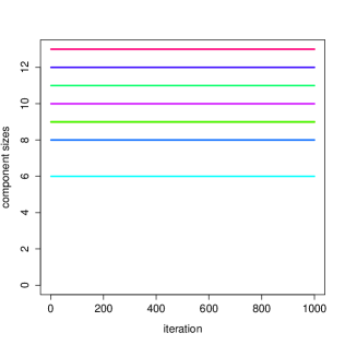
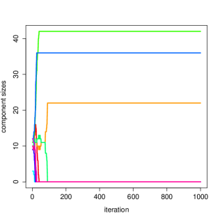
Figure 5: Trace plot of the number of observations assigned to the 10 components during MCMC sampling (each line corresponds to a component), under the prior used in Malsiner-Walli et al. (2016) with $e_{0}=0.01$ fixed (left-hand side) and under the prior setting according to the determinant criterion (right-hand side).

As a consequence, in the classification step of the sampler (see Step 1 of Algorithm 1), where an observation is assigned to the different components according to the evaluated component densities, barely any movement can be observed due to the missing overlap: once an observation is assigned to a component, it is extremely unlikely that it is allocated to another component in the next iteration.

To overcome this curse of dimensionality, a promising idea is to encourage a priori “flat”  component densities towards achieving a stronger overlapping of them also in higher dimensions. To this aim, we propose to specify the prior on the component covariances $\Sigma_{g}\sim\mathcal{W}^{-1}(c_{0},C_{0})$ such that a priori the ratio of the volume $|\Sigma_{g}|$ with respect to the total data spread $|\mbox{\rm Cov}(y)|$ is kept constant across the dimensions. Using $\mbox{\rm E}(\Sigma_{g})=C_{0}/(c_{0}-1)$, the specification of the scale matrix $C_{0}$ determines the prior expectation of $\Sigma_{g}$. In the following subsection, guidance is given how to select $C_{0}$ in order to obtain a constant ratio $|\Sigma_{g}|/|\mbox{\rm Cov}(y)|$.

Table 2: Overlap of components two and three in mixture (4) for increasing dimension $d$

dimension $d$	overlap
$2$	$0.034$
$4$	$0.003$
$50$	$2.48\cdot 10^{-6}$
$100$	$7.34\cdot 10^{-51}$
$200$	$7.21\cdot 10^{-100}$

5.1 Determinant coefficient of determination

Consider the usual inverse Whishart prior $\Sigma_{g}^{-1}\sim\mathcal{W}(c_{0},C_{0})$, where $c_{0}=\nu+(d-1)/2$, with $\nu>0$ being fixed. In this subsection, we discuss the choice of $C_{0}$ for high-dimensional mixtures.

We define $C_{0}=\phi S_{y}$, with $S_{y}$ being the empirical covariance matrix of the data, as suggested in Bensmail et al. (1997), among others, and exploit the variance decomposition of a multivariate mixture of normals, outlined in Frühwirth-Schnatter (2006):

$$\mbox{\rm Cov}(y)=\sum_{g=1}^{G}\eta_{g}\Sigma_{g}+\sum_{g=1}^{G}\eta_{g}(\mu_{g}-\mbox{\rm E}(y))(\mu_{g}-\mbox{\rm E}(y))^{\top}.$$ (5)

Thus the total variance $\mbox{\rm Cov}(y)$ of a mixture distribution with $G$ components arises from two sources of variability, namely the within-group heterogeneity, generated by the component variances $\Sigma_{g}$, and between-group heterogeneity, generated by the spread of the component means $\mu_{g}$ around the overall mixture mean $\mbox{\rm E}(y)$.

To measure how much variability may be attributed to unobserved between-group heterogeneity, Frühwirth-Schnatter (2006) considers the following two coefficients of determination derived from (5), namely the trace criterion $R^{2}_{tr}$ and the determinant criterion $R^{2}_{det}$:

$$R^{2}_{tr} = 1-\frac{\mbox{\rm tr}(\sum_{g=1}^{G}\eta_{g}\Sigma_{g})}{\mbox{\rm tr}(\mbox{\rm Cov}(y))},$$ (6)

$$R^{2}_{det} = 1-\frac{|\sum_{g=1}^{G}\eta_{g}\Sigma_{g}|}{|\mbox{\rm Cov}(y)|}.$$ (7)

Frühwirth-Schnatter (2006, p. 170) suggests to choose $\phi$ in $C_{0}=\phi S_{y}$ such that a certain amount of explained heterogeneity according to the trace criterion $R^{2}_{tr}$ is achieved:

$$\phi_{tr}=(1-\mbox{\rm E}(R^{2}_{tr}))(c_{0}-(d+1)/2)\,.$$ (8)

For instance, if $c_{0}=2.5+(d-1)/2$, then choosing 50 percent of expected explained heterogeneity yields $\phi_{tr}=0.75$, while choosing a higher percentage of explained heterogeneity such as $R^{2}_{tr}=2/3$ yields $\phi_{tr}=0.5$. Obviously, the scaling factor $\phi_{tr}$ in (8) is independent of the dimension $d$ of the data. However, the experiments in Section 4 show that this criterion yields poor clustering solutions in high dimensions such as $d=50$.

In this section, we show that choosing $\phi$ according to the determinant criterion $R^{2}_{det}$ given in (7) yields a scale matrix $C_{0}$ in the prior of the covariance matrix $\Sigma_{g}$ which increases as $d$ increases. The determinant criterion $R^{2}_{det}$ also measures the volume of the corresponding matrices which leads to a more sensible choice in a model-based clustering context.

If we substitute in (7) the term $\sum\eta_{g}\Sigma_{g}$ by the prior expected value $\Sigma_{\tilde{g}}$, with $\tilde{g}$ being an arbitrary component, and estimate $\mbox{\rm Cov}(y)$ through $S_{y}$, then we obtain

$$R^{2}_{det}=1-\frac{1}{|\Sigma^{-1}_{\tilde{g}}S_{y}|}=1-\frac{\phi_{det}^{d}}{|W|},$$

where $W\sim\mathcal{W}(c_{0},I)$. Taking the expectation,

$$\mbox{\rm E}(R^{2}_{det})=1-\phi_{det}^{d}\mbox{\rm E}(|W^{-1}|),$$

and using

$$\mbox{\rm E}(1/|W|^{a})=\frac{\Gamma_{d}(c_{0}-a)}{\Gamma_{d}(c_{0})},$$

where

$$\Gamma_{d}(c)=\pi^{d(d-1)/4}\prod_{j=1}^{d}\Gamma\left(\frac{2c+1-j}{2}\right)$$

is the generalized Gamma function, we obtain a scaling factor $\phi_{det}$ which depends on the dimension $d$ of the data:

$$\phi_{det}=(1-R^{2}_{det})^{\frac{1}{d}}\frac{\Gamma_{d}(c_{0})}{\Gamma_{d}(c_{0}-1)}.$$ (9)

Hence, the modified prior on $\Sigma_{g}^{-1}$ reads:

$$\begin{aligned} \Sigma_{g}^{-1}&\sim\mathcal{W}(c_{0},\phi_{det}S_{y}),\end{aligned}$$ (10)

where $c_{0}=2.5+(d-1)/2$, $S_{y}$ is the empirical covariance matrix of the data, and $\phi_{det}$ is given by (9). Table 3 reports $\phi_{det}$ for selected values of $d$ and $R^{2}_{det}$. Note that for this prior $C_{0}=\phi_{det}S_{y}$ is set to this fixed value, i.e. no hyperprior on $C_{0}$ is specified.

Table 3: $\phi_{det}$ for selected values of $d$ and $R^{2}_{det}$ with $c_{0}=2.5+(d-1)/2$

	$d=2$	$d=4$	$d=50$	$d=100$	$d=150$	$d=200$
$R^{2}_{det}=0.50$	1.225	1.831	11.09	20.55	29.90	39.22
$R^{2}_{det}=0.67$	0.995	1.651	11.00	20.46	29.82	39.14
$R^{2}_{det}=0.75$	0.866	1.540	10.94	20.41	29.77	39.08
$R^{2}_{det}=0.90$	0.548	1.225	10.74	20.22	29.59	38.90

5.2 Simulation study using the determinant criterion

In order to evaluate whether the proposed determinant criterion for selecting $C_{0}$ enables the Gibbs sampler to converge to the true number of components, a simulation study is performed. 100 data sets are sampled from the three-component mixture given in (4), with dimensionality $d$ varying from $2$ to $200$.

A sparse finite mixture model is fitted to the data sets using the Gibbs sampler and priors as described in Malsiner-Walli et al. (2016), however, the following prior modifications are made. The scale parameter of the Wishart prior on $\Sigma_{k}^{-1}$ is set to $C_{0}=\phi_{det}S_{y}$ as in (10) where $\phi_{det}$ is selected according (9) with $R_{det}^{2}=0.5$, see also the first row in Table 3. This corresponds to a prior proportion of heterogeneity explained by the component means of $R^{2}\approx 0.67$. The Dirichlet parameter $e_{0}$ is fixed to $0.01$ and we increase the maximum number $G$ of components to $G=30$.

The shrinkage factor $\lambda_{l}$ in the prior specification (3) is fixed to $1$, since all variables $y_{il}$ are relevant for clustering in the present context. By design, for each single variable $y_{il}$ two of the means $\mu_{l1},\mu_{l2},\mu_{l3}$ are different. Furthermore, all pairs of variables $(y_{il},y_{i,l+2})$ exhibit three well-separated component means located at (1,1), (4,4), (1,4) or (4,1) in their bivariate marginal distribution $p(y_{il},y_{i,l+2})$. Hence, none of the variables is irrelevant in the sense that $\mu_{l1}\approx\mu_{l2}\approx\mu_{l3}$.

The estimated number of components is reported in Table 4, based on an Gibbs sampling with $T=8,000$ iterations after discarding the first $800$ iterations as burn-in for each of the 100 data sets. For $n=1,000$ and $n=10,000$, the resulting clustering is almost perfect, even for very high dimensions such as $d=200$. The Gibbs sampler converges to the true number of components, as can be seen in the trace plot on the right-hand side of Figure 5, by leaving all specified components but three empty. For small data sets with $n=100$, the criterion leads to an underfitting solution ($\hat{G}=2$) for small $d$. However, as can be seen in the left-hand scatter plot in Figure 4, a small data set of only 100 observations may not contain enough information for estimating three groups. Also, if $d>n$ the mixture model is not well-defined, and the Gibbs sampler gets stuck again. However, for $d=50$ and $d=100$ the approach works well also for small data sets with $n=100$.

Table 4: Clustering results of the simulation study involving an increasing number of $d$ variables and $n$ observations, based on 100 simulated data sets for each combination of $n$ and $d$. The prior on $\Sigma_{k}^{-1}$ is chosen as in (10) with $C_{0}=\phi_{det}S_{y}$ and $R^{2}_{det}=0.50$. The most frequently visited number of clusters $\tilde{G}$ (with frequencies in parentheses), the posterior mean of the number of clusters $\hat{G}$ and the adjusted Rand index $r_{a}$ are averaged across the 100 simulated data sets

		$n=100$			$n=1,000$			$n=10,000$
$d$	${\phi}_{det}$	$\tilde{G}$	$\hat{G}$	$r_{a}$	$\tilde{G}$	$\hat{G}$	$r_{a}$	$\tilde{G}$	$\hat{G}$	$r_{a}$
$2$	$1.23$	2(93)	2.0	0.45	3(100)	3.0	0.73	3(98)	3.0	0.75
$4$	$1.83$	2(70)	2.3	0.69	3(100)	3.0	0.93	3(100)	3.0	0.93
$50$	$11.09$	3(100)	3.0	1.00	3(100)	3.0	1.00	3(100)	3.0	1.00
$100$	$20.55$	3(100)	3.0	1.00	3(100)	3.0	1.00	3(100)	3.0	1.00
$150$	$29.90$	3(85)	3.5	0.99	3(100)	3.0	1.00	3(100)	3.0	1.00
$200$	$39.22$	3(31)	10.7	0.77	3(97)	3.1	0.99	3(100)	3.0	1.00

6 Concluding Remarks

This chapter discussed practical Bayesian inference for finite mixtures using sampling based methods. While these methods work well for moderately sized mixtures, Gibbs sampling turned out to be the only operational method for handling high-dimensional mixtures. Based on a simulation study, aiming at estimating Gaussian mixture models with fifty variables, we were unable to tune commonly used algorithms such as the Metropolis-Hastings algorithm or sequential Monte Carlo, due to the curse of dimensionality. Gibbs sampling turned out to be the exception in this collection of algorithms. However, we also found out that the Gibbs sampler may get stuck when initialized with many small data clusters under previously published priors.

Hence, we consider that calibrating prior parameters in high-dimensional spaces remains a delicate issue. For Gaussian mixtures, we examined the role of the determinant criterion introduced by Frühwirth-Schnatter (2006) for incorporating the prior expected proportion of heterogeneity explained by the component means (and thereby determining the heterogeneity covered by the components themselves). This led us to a new choice of the scaling matrix in the inverse Wishart prior. The resulting prior, in combination with Gibbs sampling, worked quite well, when estimating the number of components for Gaussian mixtures, even for very high-dimensional data sets with 200 variables. Starting with a strongly overfitted mixture, the Gibbs sampler was able to converge to the true model.

Many other computational issues deserve further investigation, in particular for mixture models for high-dimensional data. Additionally to the ’big $p$’ (in our notation ’big $d$’) and to the ’big $n$’ problem, the ’big $G$’ problem is also relevant. Are we able to estimate several tens data clusters or more, a case that arises in high-energy physics, see Frühwirth et al. (2016) or genomics, see Rau and Maugis-Rabusseau (2018)?

References

- Behboodian (1972) Behboodian J (1972). “Information matrix for a mixture of two normal distributions.” Journal of Statistical Computation and Simulation, 1(4), 295–314.
- Bensmail et al. (1997) Bensmail H, Celeux G, Raftery A, Robert C (1997). “Inference in model-based cluster analysis.” Statistics and Computing, 7(1), 1–10.
- Berkhof et al. (2003) Berkhof J, van Mechelen I, Gelman A (2003). “A Bayesian approach to the selection and testing of mixture models.” Statistica Sinica, 13, 423–442.
- Bernardo and Girón (1988) Bernardo JM, Girón FJ (1988). “A Bayesian analysis of simple mixture problems.” In JM Bernardo, MH DeGroot, DV Lindley, AFM Smith (eds.), Bayesian Statistics 3, pp. 67–78. Oxford University Press, Oxford.
- Buchner (2014) Buchner J (2014). “A statistical test for nested sampling algorithms.” Preprint, arXiv:1407.5459.
- Cappé et al. (2004) Cappé O, Moulines E, Rydén T (2004). Hidden Markov Models. Springer-Verlag, New York.
- Celeux et al. (2000) Celeux G, Hurn M, Robert C (2000). “Computational and inferential difficulties with mixture posterior distributions.” Journal of the American Statistical Association, 95, 957–979.
- Chib (1995) Chib S (1995). “Marginal likelihood from the Gibbs output.” Journal of the American Statistical Association, 90, 1313–1321.
- Chopin (2002) Chopin N (2002). “A sequential particle filter method for static models.” Biometrika, 89, 539–552.
- Chopin (2004) Chopin N (2004). “Central Limit theorem for sequential Monte Carlo methods and its application to Bayesian inference.” Annals of Statistics, 32(6), 2385–2411.
- Chopin and Robert (2010) Chopin N, Robert C (2010). “Properties of nested sampling.” Biometrika, 97, 741–755.
- Crawford et al. (1992) Crawford S, DeGroot MH, Kadane J, Small MJ (1992). “Modelling lake-chemistry distributions: Approximate Bayesian methods for estimating a finite-mixture model.” Technometrics, 34, 441–453.
- Del Moral et al. (2006) Del Moral P, Doucet A, Jasra A (2006). “Sequential Monte Carlo samplers.” Journal of the Royal Statistical Society, Series B, 68(3), 411–436.
- Dickey (1968) Dickey JM (1968). “Three multidimensional integral identities with Bayesian applications.” Annals of Statistics, 39, 1615–1627.
- Diebolt and Robert (1990a) Diebolt J, Robert C (1990a). “Bayesian estimation of finite mixture distributions, Part I: Theoretical aspects.” Technical Report 110, LSTA, Université Paris VI, Paris.
- Diebolt and Robert (1990b) Diebolt J, Robert C (1990b). “Estimation des paramètres d’un mélange par échantillonnage bayésien.” Notes aux Comptes-Rendus de l’Académie des Sciences I, 311, 653–658.
- Diebolt and Robert (1994) Diebolt J, Robert C (1994). “Estimation of finite mixture distributions by Bayesian sampling.” Journal of the Royal Statistical Society, Series B, 56, 363–375.
- Everitt et al. (2016) Everitt RG, Culliford R, Medina-Aguayo F, Wilson DJ (2016). “Sequential Bayesian inference for mixture models and the coalescent using sequential Monte Carlo samplers with transformations.” Preprint, arXiv:1612.06468.
- Feroz et al. (2013) Feroz F, Hobson MP, Cameron E, Pettitt AN (2013). “Importance nested sampling and the MultiNest algorithm.” Preprint, arXiv:1306.2144.
- Frühwirth et al. (2016) Frühwirth R, Eckstein K, Frühwirth-Schnatter S (2016). “Vertex finding by sparse model-based clustering.” Journal of Physics: Conference Series, 762, 012055. URL http://stacks.iop.org/1742-6596/762/i=1/a=012055.