Weakly informative reparameterisations for location-scale mixtures

Abstract

While mixtures of Gaussian distributions have been studied for more than a century, the construction of a reference Bayesian analysis of those models remains unsolved, with a general prohibition of improper priors (Frühwirth-Schnatter, 2006) due to the ill-posed nature of such statistical objects. This difficulty is usually bypassed by an empirical Bayes resolution (Richardson and Green, 1997). By creating a new parameterisation centred on the mean and possibly the variance of the mixture distribution itself, we manage to develop here a weakly informative prior for a wide class of mixtures with an arbitrary number of components. We demonstrate that some posterior distributions associated with this prior and a minimal sample size are proper. We provide MCMC implementations that exhibit the expected exchangeability. We only study here the univariate case, the extension to multivariate location-scale mixtures being currently under study. An R package called Ultimixt is associated with this paper.

Keywords: Non-informative prior, improper prior, mixture of distributions, Bayesian analysis, Dirichlet prior, exchangeability, polar coordinates, compound distributions.

1 Introduction

A mixture density is traditionally represented as a weighted average of densities from standard families, i.e.,

$$f(x|\boldsymbol{\theta},\mathbf{p})=\sum_{i=1}^{k}p_{i}f_{i}(x|\theta_{i})\qquad\sum_{i=1}^{k}p_{i}=1\,.$$ (1)

Each component of the mixture is characterised by a component-wise parameter $\theta_{i}$ and the weights $p_{i}$ of those components translate the importance of each of those components in the model. A more general if rarely considered mixture model involves different families for the different components.

This particular representation 1 gives a separate meaning to each component through its parameter $\theta_{i}$, even though there is a well-known lack of identifiability in such models, due to the invariance of the sum by permutation of the indices. This issue relates to the equally well-known “label switching” phenomenon in the Bayesian approach to the model, which pertains both to Bayesian inference and to simulation of the corresponding posterior (Celeux et al., 2000; Stephens, 2000b; Frühwirth-Schnatter, 2001; Jasra et al., 2005). From this Bayesian viewpoint, the choice of the prior distribution on the component parameters is quite open, the only constraint being obviously that the corresponding posterior is proper. Diebolt and Robert (1994) and Wasserman (1999) discussed the alternative approach of imposing proper posteriors on improper priors by banning almost empty components from the likelihood function. While consistent, this approach induces dependence between the observations, requires a large enough number of observations, higher computational costs, and does not handle over-fitting very well.

The prior distribution on the weights $p_{i}$ is equally open for choice, but a standard version is a Dirichlet distribution with common hyperparameter $\alpha_{0}$, $\text{Dir}(\alpha_{0},\ldots,,\alpha_{0})$.  Recently, Rousseau and Mengersen (2011b) demonstrated that the choice of this hyperparameter $\alpha_{0}$ relates to the inference on the total number of components, namely that a small enough value of $\alpha_{0}$ manages to handle over-fitted mixtures in a convergent manner. In Bayesian non-parametric modelling, Griffin (2010) showed that the prior on the weights may have a higher impact when inferring about the number of components, relative to the prior on the component-specific parameters. As indicated above, the prior distribution on the $\theta_{i}$’s has received less attention and conjugate choices are most standard, since they facilitate simulation via Gibbs samplers (Diebolt and Robert, 1990; Escobar and West, 1995; Richardson and Green, 1997) if not estimation, since posterior moments remain unavailable in closed form. In addition, Richardson and Green (1997) among others proposed data-based priors that derive some hyperparameters as functions of the data, towards an automatic scaling of such priors, as illustrated by the R package, bayesm (Rossi and McCulloch, 2010).

In an objective Bayes perspective (Berger, 2004; Berger et al., 2009), we seek a prior that is minimally informative with respect to the information brought by the data. This has been formalised in different ways, including the Jeffreys prior (Jeffreys, 1939), reference priors (Berger et al., 2009), maximum entropy priors (Rissanen, 2012), matching priors (Ghosh et al., 1995), which often include Jeffreys priors (Welch and Peers, 1963), and other proposals (Kass and Wasserman, 1996). In the case of mixture models, very little has been done, apart from Bernardo and Giròn (1988), who derived the Jeffreys priors for mixtures where components have disjoint supports, Figueiredo and Jain (2002) who used independent Jeffreys prior on components, and Rubio and Steel (2014) which achieve a closed-form expression for the Jeffreys prior of a location-scale mixture with two disjoint components. Recently, Grazian and Robert (2015) undertook an analytical and numerical study of Jeffreys priors for Gaussian mixtures, which showed that Jeffreys priors are almost invariably associated with improper posteriors, whatever the sample size, and advocated the use of pseudo-priors expressed as conditional Jeffreys priors for each type of parameters. In this paper, we instead start from the traditional Jeffrey prior for a location-scale parameter to derive a joint prior distribution on all parameters by taking advantage of compact reparameterisation, which allow for uniform distributions and similarly weakly informative distributions.

In the case when $\theta_{i}=(\mu_{i},\sigma_{i})$ is a location-scale parameter, Mengersen and Robert (1996) have already proposed a reparameterisation of (1) that express each component as a local perturbation of the previous one, namely $\mu_{i}=\mu_{i-1}+\sigma_{i-1}\delta_{i}$, $\sigma_{i}=\tau_{i}\sigma_{i-1}$, $\tau_{i}<1$ $(i>1)$, with $\mu_{1}$ and $\sigma_{1}$ being the reference values. Based on this reparameterisation, Robert and Titterington (1998) established that a specific improper prior on $(\mu_{1},\sigma_{1})$ leads to a proper posterior in the Gaussian case. We propose here to modify this reparameterisation by using the mean and variance of the mixture distribution as reference location and scale, respectively. This modification has foundational consequences in terms of identifiability and hence of exploiting improper and non-informative priors for mixture models, in sharp contrast with the existing literature (see, e.g. Diebolt and Robert, 1994; Wasserman, 1999).

Computational approaches to Bayesian inference on mixtures are quite diverse, starting with the introduction of the Gibbs sampler (Diebolt and Robert, 1990; Gelman and King, 1990; Escobar and West, 1995), some concerned with approximations (Roeder, 1990; Wasserman, 1999) and MCMC features (Richardson and Green, 1997; Celeux et al., 2000), and others with asymptotic justifications, in particular when over-fitting mixtures (Rousseau and Mengersen, 2011b), but most attempting to overcome the methodological hurdles in estimating mixture models (Chib, 1995; Neal, 1999; Berkhof et al., 2003; Marin et al., 2005; Frühwirth-Schnatter, 2006; Lee et al., 2009). While we do not propose here a novel computational methodology attached with our new priors, we study the performances of several MCMC algorithms on such targets.

In this paper, we introduce and study a principle of mean-variance or simply mean reparameterisation (Section 2), which main consequence is to constrain all parameters but mean and variance of the overall mixture model within a compact space. We study several possible parameterisations of that kind and demonstrate that an improper Jeffreys-like prior associated with them is proper for a wide variety of mixture and compound mixture distributions. Taking advantage of constraints on component-wise parameters, a domain based prior is used. Section 2.4 discusses some properties of the resulting priors in terms of the modelled densities. In Section 3, we propose some MCMC implementations to estimate the parameters of the mixture, discussing label switching (Section 3.3). Note that a public R package called Ultimixt is associated with this approach. Section 4 describes several case studies when implementing the reparameterisation principle, and Section 5 briefly concludes the paper. Proofs of the main results are available in the Supplementary Material.

2 Mixture reparameterisation

2.1 Mean and variance of a mixture

Let us first recall how both mean and variance of a mixture distribution with finite first two moments can be represented in terms of the mean and variance parameters of the components of the mixture.

Lemma 1

If $\mu_{i}$ and $\sigma_{i}^{2}$ are well-defined as mean and variance of the distribution with density $f_{i}(\cdot|\theta_{i})$, respectively, the mean of the mixture distribution (1) is given by

$$\mathbb{E}_{\boldsymbol{\theta},\mathbf{p}}[X]=\sum_{i=1}^{k}p_{i}\mu_{i}$$

and its variance by

$${\mathrm{var}}_{\boldsymbol{\theta},\mathbf{p}}(X)=\sum_{i=1}^{k}p_{i}\sigma_{i}^{2}+\sum_{i=1}^{k}p_{i}(\mu_{i}^{2}-\mathbb{E}_{\boldsymbol{\theta},\mathbf{p}}[X]^{2})$$

For any location-scale mixture, we propose a reparameterisation of the mixture model that starts by scaling all parameters in terms of its global mean $\mu$ and global variance $\sigma^{2}$. For instance, we can switch from the parameterisation in $(\mu_{i},\sigma_{i})$ to a new parameterisation in $(\mu,\sigma,\alpha_{1},\ldots,\alpha_{k},\tau_{1},\ldots,\tau_{k},p_{1},\ldots,p_{k})\,,$ expressing those component-wise parameters as

$$\mu_{i}=\mu+\sigma\alpha_{i}\quad\text{ and }\quad\sigma_{i}=\sigma\tau_{i}\qquad 1\leq i\leq k$$ (2)

where $\tau_{i}>0$ and $\alpha_{i}\in\mathbb{R}$. This bijective reparameterisation is similar to the one in Mengersen and Robert (1996), except that these authors put no special meaning on their location and scale parameters, which are then non-identifiable. Once $\mu$ and $\sigma$ are defined as (global) mean and variance of the mixture distribution, eqn. (2) imposes compact constraints on the other parameters of the model. For instance, since the mixture variance is equal to $\sigma^{2}$, this implies that $(\mu_{1},\ldots,\mu_{k},\sigma_{1},\ldots,\sigma_{k})$ belongs to an ellipse conditional on the weights, $\mu$, and $\sigma$, by virtue of Lemma 1.

Considering the $\alpha_{i}$’s and the $\tau_{i}$’s in (2) as the new and local parameters of the mixture components, the following result (Lemma 2) states that the global mean and variance parameters are the sole freely varying parameters. In other words, once both the global mean and variance are defined as such, there exists a parameterisation such that all remaining parameters of a mixture distribution are restricted to belong to a compact set, a feature that is most helpful in selecting a non-informative prior distribution.

Lemma 2

The parameters $\alpha_{i}$ and $\tau_{i}$ in (2) are constrained by

$$\sum_{i=1}^{k}p_{i}\alpha_{i}=0\quad{\mbox{a}nd}\quad\sum_{i=1}^{k}p_{i}\tau_{i}^{2}+\sum_{i=1}^{k}p_{i}\alpha_{i}^{2}=1\,.$$

The same concept applies for other families, namely that one or several moments of the mixture distribution can be used as a pivot to constrain the component parameters. For instance, a mixture of exponential distributions $\mathcal{E}(\lambda_{i}^{-1})$ or a mixture of Poisson distributions $\mathcal{P}(\lambda_{i})$ can be reparameterised in terms of its mean, $\mathbb{E}[X]$, through the constraint

$$\mathbb{E}[X]=\lambda=\sum_{i=1}^{k}p_{i}\lambda_{i},$$

by introducing the parameterisation $\lambda_{i}=\lambda\gamma_{i}/p_{i}$, $\gamma_{i}>0$, which implies $\sum_{i=1}^{k}\gamma_{i}=1$. As detailed below, this notion immediately extends to mixtures of compound distributions, which are scale perturbations of the original distributions, with a fixed distribution on the scales.

2.2 Proper posteriors of improper priors

The constraints in Lemma 2 define a set of values of $(p_{1},\ldots,p_{k},\alpha_{1},\ldots,\alpha_{k},\tau_{1},\ldots,\tau_{k})$ that is obviously compact. One sensible modelling approach exploiting this feature is to resort to uniform or other weakly informative proper priors for those component-wise parameters, conditional on $(\mu,\sigma)$. Furthermore, since $(\mu,\sigma)$ is a location-scale parameter, we invoke Jeffreys (1939) to choose a Jeffreys-like prior $\pi(\mu,\sigma)=1/\sigma$ on this parameter, even though we stress this is not the genuine (if ineffective) Jeffreys prior for the mixture model (Grazian and Robert, 2015). In the same spirit as Robert and Titterington (1998), we now establish that this choice of prior produces a proper posterior distribution for a minimal sample size of two.

Theorem 1

The posterior distribution associated with the prior $\pi(\mu,\sigma)=1/\sigma$ and with the likelihood derived from (1) is proper when the components $f_{1}(\cdot|\mu,\sigma),\dots,f_{k}(\cdot|\mu,\sigma)$ are Gaussian densities, provided (a) prior distributions on the other parameters are proper and independent of $(\mu,\sigma)$, and (b) there are at least two observations in the sample.

While only handling the Gaussian case is a limitation, the above result extends to mixtures of compound Gaussian distributions, which are defined as scale mixtures, namely $X=\mu+\sigma\xi Z$, $Z\sim\mathrm{N}(0,1)$ and $\xi\sim h(\xi)$, when $h$ is a probability distribution on $\mathbb{R}^{+}$ with second moment equal to $1$. (The moment constraint ensures that the mean and variance of this compound Gaussian distribution are $\mu$ and $\sigma^{2}$, respectively.) As shown by Andrews and Mallows (1974), by virtue of Bernstein’s theorem, such compound Gaussian distributions are identified as completely monotonous functions and include a wide range of probability distributions like the $t$, the double exponential, the logistic, and the $\alpha$-stable distributions (Feller, 1971).

Corollary 1

The posterior distribution associated with the prior $\pi(\mu,\sigma)=1/\sigma$ and with the likelihood derived from (1) is proper when the component densities $f_{i}(\cdot|\mu,\sigma)$ are all compound Gaussian densities, provided (a) prior distributions on the other parameters are proper and independent of $(\mu,\sigma)$ and (b) there are at least two observations in the sample.

The proof of this result is a straightforward generalisation of the one of Theorem 1, which involves integrating out the compounding variables $\xi_{1}$ and $\xi_{2}$ over their respective distributions. Note that the mixture distribution (1) allows for different classes of location-scale distributions to be used in the different components.

If we now consider the case of a Poisson mixture,

$$f(x|\lambda_{1},\ldots,\lambda_{k})=\frac{1}{x!}\sum_{i=1}^{k}p_{i}\lambda_{i}^{x}e^{-\lambda_{i}}$$ (3)

with a reparameterisation as $\lambda=\mathbb{E}[X]$ and $\lambda_{i}=\lambda\gamma_{i}/p_{i}$, we can use the equivalent to the Jeffreys prior for the Poisson distribution, namely, $\pi(\lambda)=1/\lambda$, since it leads to a well-defined posterior with a single positive observation.

Theorem 2

The posterior distribution associated with the prior $\pi(\lambda)=1/\lambda$ and with the Poisson mixture (3) is proper provided (a) prior distributions on the other parameters are proper and independent of $\lambda$ and, (b) there is at least one strictly positive observation in the sample.

Once again, this result straightforwardly extends to mixtures of compound Poisson distributions, namely distributions where the parameter is random with mean $\lambda$:

$$\mathbb{P}(X=x|\lambda)=\int\frac{1}{x!}(\lambda\xi)^{x}\exp\{-\lambda\xi\}\,\text{d}\nu(\xi)\,,$$

with the distribution $\nu$ possibly discrete. In the special case when $\nu$ is on the integers, this representation covers all infinitely exchangeable distributions (Feller, 1971).

Corollary 2

The posterior distribution associated with the prior $\pi(\lambda)=1/\lambda$ and with the likelihood derived from a mixture of compound Poisson distributions is proper provided (a) prior distributions on the other parameters are proper and independent to $\lambda$ and, (b) there is at least one strictly positive observation in the sample.

Another instance of a proper posterior distribution is provided by exponential mixtures,

$$f(x|\lambda_{1},\ldots,\lambda_{k})=\sum_{i=1}^{k}\frac{p_{i}}{\lambda_{i}}e^{-\nicefrac{{x}}{{\lambda_{i}}}}\,,$$ (4)

since a reparameterisation via $\lambda=\mathbb{E}[X]$ and $\lambda_{i}=\lambda\gamma_{i}/p_{i}$ leads to the posterior being well-defined for a single observation.

Theorem 3

The posterior distribution associated with the prior $\pi(\lambda)=1/\lambda$ and with the likelihood derived from the exponential mixture (4) is proper provided proper distributions are used on the other parameters.

Once again, this result directly extends to mixtures of compound exponential distributions, namely exponential distributions where the parameter is random with mean $\lambda$:

$$f(x|\lambda)=\int\frac{1}{\lambda\xi}\exp\{-\nicefrac{{x}}{{\lambda\xi}}\}\,\text{d}\nu(\xi)\,,\quad x>0\,.$$

In particular, this representation contains all Gamma distributions with shape less than one (Gleser, 1989) and Pareto distributions (Klugman et al., 2004).

Corollary 3

The posterior distribution associated with the prior $\pi(\lambda)=1/\lambda$ and with the likelihood derived from a mixture of compound exponential distributions is proper provided proper distributions are used on the other parameters.

The parameterisation (2) is one of many of a Gaussian mixture. In practice, one could design a normal and a inverse-gamma distribution as priors for $\alpha_{i}$ and $\tau_{i}$, respectively, and make those priors vague via the choice of hyperparameters derived from the standardised data (borrowing the idea by Rossi and McCulloch (2010)). This would make the prior on local parameters a data-based prior and consequently the marginal prior for $\mu_{i}$ and $\sigma_{i}$ would also be a data-based prior. A fundamental difficulty with this scheme is that the constraints found in Lemma 2 are incompatible with this independent modelling to each other. We are thus seeking another parameterisation of the mixture that allows for a natural and weakly informative prior (hence not based on the data) while incorporating the constraints. This is the purpose of the following sections.

2.3 Further reparameterisations in location-scale models

We are now building a reparameterisation that will handle the constraints of Lemma 2 in such a way as to allow for manageable uniform priors on the resulting parameter set. Exploiting the form of the constrains, we can rewrite the component location and scale parameters in (2) as $\alpha_{i}=\gamma_{i}/\sqrt{p_{i}}$ and $\tau_{i}=\eta_{i}/\sqrt{p_{i}}\,,$ leading to the mixture representation

$$f(x|\boldsymbol{\theta},\mathbf{p})=\sum_{i=1}^{k}p_{i}f_{i}(x|\mu+\sigma\gamma_{i}/\sqrt{p_{i}},\sigma\eta_{i}/\sqrt{p_{i}})\,,\quad\eta_{i}>0\,,$$ (5)

Given the weight vector $(p_{1},\cdots,p_{k})$, these new parameters are constrained by

$$\sum_{i=1}^{k}\sqrt{p_{i}}\gamma_{i}=0\quad\text{and }\quad\sum_{i=1}^{k}(\eta_{i}^{2}+\gamma_{i}^{2})=1\,,$$ (6)

which means that $(\gamma_{1},\ldots,\gamma_{k},\eta_{1},\ldots,\eta_{k})$ belongs both to a hyper-sphere of $\mathbb{R}^{2k}$ and to a hyperplane of this space, hence to the intersection between both. Since the supports of $\eta_{i}$ and $\gamma_{i}$ are bounded (i.e., $0\leq\eta_{i}\leq 1$ and $-1\leq\gamma_{i}\leq 1$), any proper distribution with the appropriate support can be used as prior and extracting knowledge from the data is not necessary to build vague priors as in Richardson and Green (1997).

Given these new constraints, the parameter set remains complex and the ensuing construction of a prior still is delicate. We can however proceed towards Dirichlet style distributions on the parameter. First, mean and variance parameters in (5) can be separated by introducing a supplementary parameter, namely a radius $\varphi$ such that

$$\sum_{i=1}^{k}\gamma_{i}^{2}=\varphi^{2}\quad\text{ and }\quad\sum_{i=1}^{k}\eta_{i}^{2}=1-\varphi^{2}\,.$$ (7)

This decomposition of the spherical constraint then naturally leads to a hierarchical prior where, for instance, $\varphi^{2}$ and $(p_{1},\ldots,p_{k})$ are distributed as $\mathcal{B}e(a_{1},a_{2})$ and $\mathcal{D}ir(\alpha_{0},\ldots,\alpha_{0})$ variates, respectively, while the vectors $(\gamma_{1},\ldots,\gamma_{k})$ and $(\eta_{1},\ldots,\eta_{k})$ are uniformly distributed on the spheres of radius $\varphi$ and $\sqrt{1-\varphi^{2}}$, respectively, under the additional linear constraint $\sum_{i=1}^{k}\sqrt{p_{i}}\gamma_{i}=0$.

Since this constraint is an hindrance for easily simulating the $\gamma_{i}$’s, we now complete the move to a new parameterisation, based on spherical coordinates, which can be handled most straightforwardly.

2.3.1 Spherical coordinate representation of the $\gamma$’s

In equations (6), the vector $(\gamma_{1},\ldots,\gamma_{k})$ belongs both to the hyper-sphere of radius $\varphi$ and to the hyperplane orthogonal to $(\sqrt{p_{1}},\ldots,\sqrt{p_{k}})$. Therefore, $(\gamma_{1},\ldots,\gamma_{k})$ can be expressed in terms of its spherical coordinates within that hyperplane. Namely, if $(\digamma_{1},\ldots,\digamma_{k-1})$ denotes an orthonormal basis of the hyperplane, $(\gamma_{1},\ldots,\gamma_{k})$ can be written as

$$(\gamma_{1},\ldots,\gamma_{k})=\varphi\cos(\varpi_{1})\digamma_{1}+\varphi\sin(\varpi_{1})\cos(\varpi_{2})\digamma_{2}+\ldots+\varphi\sin(\varpi_{1})\cdots\sin(\varpi_{k-2})\digamma_{k-1}$$

with the angles $\varpi_{1},\ldots,\varpi_{k-3}$ in $[0,\pi]$ and $\varpi_{k-2}$ in $[0,2\pi]$. The $s$-th orthonormal base $\digamma_{s}$ can be derived from the $k$-dimensional orthogonal vectors $\widetilde{\digamma}_{s}$ where

$$\widetilde{\digamma}_{1,j}=\Bigg{\{}\begin{array}[]{c c l}-\sqrt{p_{2}},&&j=1\\ \sqrt{p_{1}},&&j=2\\ 0,&&j>2\end{array}$$

and the $s$-th vector is given by $(s>1)$

$$\widetilde{\digamma}_{s,j}=\left\{\begin{array}[]{c c l}-(p_{j}p_{s+1})^{1/2}\Big{/}\left(\displaystyle\sum\nolimits^{s}_{l=1}p_{l}\right)^{1/2},&&j\leq s\\ \left(\displaystyle\sum\nolimits^{s}_{l=1}p_{l}\right)^{1/2},&&j=s+1\\ 0,&&j>s+1\end{array}\right.$$

Note the special case when $k=2$ when the angle $\varpi_{1}$ is missing. In this case, the mixture location parameter is then defined by $(\gamma_{1},\gamma_{2})=\varphi\digamma_{1}$ and $\varphi$ takes both positive and negative values. In the general case, the parameter vector $(\gamma_{1}\cdots,\gamma_{k})$ is a bijective transform of $(\varphi^{2},p_{1},\cdots,p_{k},\varpi_{1},\cdots,\varpi_{k-2})$.

This reparameterisation achieves the intended goal, since a natural reference prior for $\varpi$ is made of uniforms, $(\varpi_{1},\cdots,\varpi_{k-3})\sim\mathcal{U}([0,\pi]^{k-3})$, and $\varpi_{k-2}\sim\mathcal{U}[0,2\pi]$, although other choices are obviously possible and should be explored to test the sensitivity to the prior. Prior distributions on the other parameterisations we encountered can then be derived by a change of variables.

2.3.2 Dual spherical representation of the $\eta_{i}$’s

The vector of the component variance parameters $(\eta_{1},\cdots,\eta_{k})$ belongs to the $k$-dimension sphere of radius $\sqrt{1-\varphi^{2}}$. A natural prior is a Dirichlet distribution with common hyperparameter $a$,

$$\pi(\eta_{1}^{2},\cdots,\eta^{2}_{k},\varphi^{2})=\mathcal{D}ir(\alpha,\cdots,\alpha)$$

For $k$ small enough, $(\eta_{1},\cdots,\eta_{k})$ can easily be simulated from the corresponding posterior. However, as $k$ increases, sampling may become more delicate by a phenomenon of concentration of the posterior distribution and it benefits from a similar spherical reparameterisation. In this approach, the vector $(\eta_{1},\cdots,\eta_{k})$ is also rewritten through spherical coordinates with angle components $(\xi_{1},\cdots,\xi_{k-1})$,

$$\eta_{i}=\left\{\begin{array}[]{l c}\sqrt{1-\varphi^{2}}\cos(\xi_{i})\,,&i=1\\ \sqrt{1-\varphi^{2}}\displaystyle\prod^{i-1}_{j=1}\sin(\xi_{j})\cos(\xi_{i})\,,&1<i<k\\ \sqrt{1-\varphi^{2}}\displaystyle\prod^{i-1}_{j=1}\sin(\xi_{j})\,,&i=k\end{array}\right.$$

Unlike $\varpi$, the support for all angles $\xi_{1},\cdots,\xi_{k-1}$ is limited to $[0,\pi/2]$, due to the positivity requirement on the $\eta_{i}$’s. In this case, a reference prior on the angles is $(\xi_{1},\cdots,\xi_{k-1})\sim\mathcal{U}([0,\pi/2]^{k-1})\,,$ while obviously alternative choices are possible.

2.4 Weakly informative priors for Gaussian mixture models

The above introduced two new parameterisations of a Gaussian mixture model, based on equation (5) and its spherical representations in Sections 2.3.1 and 2.3.2. Under the constraints imposed by the first two moment -parameters, two weakly informative priors, called the (i) single and (ii) double uniform priors, are considered below and their impact on the resulting marginal prior distributions is studied.

For the parameterisation constructed in Section 2.3.1, $\gamma$ is expressed in terms of its spherical coordinates over the $k-1$ subset, uniformly distributed over $[0,\pi]^{k-3}\times[0,2\pi]$, and $\eta$ is associated with a uniform distribution over the $\mathbb{R}^{k}$ simplex, conditional on $\varphi$. This prior modelling is called the single uniform prior. Another reparametrisation is based on the spherical representations of both $\gamma$ and $\eta$ leading to the double uniform prior, a uniform distribution on all angle parameters, $\varpi_{i}$’s and $\eta_{i}$’s. Both priors can be argued to be weakly informative priors, relying on uniforms for a given parameterisation.

To evaluate the difference between both modellings, using a uniform prior on $\varphi^{2}$ and a Dirichlet distribution on the $p_{i}$’s, we generated $20,000$ samples from both priors. The resulting component-wise parameter distributions are represented in Figure 1. As expected, under the single uniform prior, all $\eta_{i}$’s and $\gamma_{i}$’s are uniformly distributed over the $k$-ball, are thus exchangeable and, as a result, all density estimates are close. When using the double uniform priors, the components are ordered through their spherical representation. As $k$ increases, the ordering becomes stronger over a wider range, when compared with the first uniform prior and the component-wise priors become more skewed away from the global mean parameter value. This behaviour is reflected in the distribution of some quantiles of the mixture model, as seen in Figure 2. When $k=3$, the supports of the mixture models are quite similar for both priors. When $k=20$, the double uniform prior tends to put more mass around the global mean of $0$, as shown by the median distribution, and it allows for mixtures with long tails more readily than the single uniform prior. Therefore, the double uniform prior is our natural choice for simulation studies in Section 4.

Figure 1: Density estimate of 20,000 draws of $\log(|\gamma_{i}/\sqrt{p_{i}}|)$ and $\log(\eta_{i}/\sqrt{p_{i}})$ from the single uniform prior (red lines) and the double uniform prior (grey lines) when $k=3$ (top) and $k=20$ (bottom). Different grey lines indicate the density estimates for $i=1,\ldots,k$.

Figure 2: Boxplot of quantiles of mixture models with 20,000 parameter values from the single and double uniform priors when $k=3$ (top) and $k=20$ (bottom). The mean of the mixture is $0$ and its variance is $1$.

3 MCMC implementations

3.1 A Metropolis-within-Gibbs sampler in the Gaussian case

Given the reparameterisations introduced in Section 2, and in particular Section 2.3 for the Gaussian mixture model, different MCMC implementations are possible and we investigate in this section some of these. To this effect, we distinguish between the single and double uniform priors.

Although the target density is not too dissimilar to the target explored by early Gibbs samplers in Diebolt and Robert (1990) and Gelman and King (1990), simulating directly the new parameters implies managing constrained parameter spaces. The hierarchical nature of the parameterisation also leads us to consider a block Gibbs sampler that coincides with this hierarchy. Since the corresponding full conditional posteriors are not in closed form, a Metropolis-within-Gibbs sampler is implemented here with random walk proposals. In this approach, the scales of the proposal distributions are automatically calibrated towards optimal acceptance rates (Roberts et al., 1997; Roberts and Rosenthal, 2001, 2009). Convergence of a simulated chain is assessed based on the rudimentary convergence monitoring technique of Gelman and Rubin (1992). The description of the algorithm is provided by a pseudo-code representation in the Supplementary Material (Figure 10). Note that the Metropolis-within-Gibbs version does not rely on latent variables and completed likelihood as in Tanner and Wong (1987) and Diebolt and Robert (1990). Following the adaptive MCMC method in Section 3 of Roberts and Rosenthal (2009), we derive the optimal scales associated with proposal densities, based on 10 batches with size 50. The scales $\epsilon$ are identified by a subscript with the corresponding parameter (see, e.g., Table 1).

For the single reparameterisation, all steps in Figure 10 are the same except that Steps 2.5 and 2.7 are ignored. When $k$ is not large, one potential proposal density for $((\varphi^{2})^{(t)},(\eta_{1}^{2})^{(t)},\ldots,(\eta_{k}^{2})^{(t)})$ is a Dirichlet distribution,

$$((\varphi^{2})^{\prime},(\eta_{1}^{2})^{\prime},\ldots,(\eta_{k}^{2})^{\prime})\sim\text{Dir}((\varphi^{2})^{(t-1)}\epsilon,(\eta_{1}^{2})^{(t-1)}\epsilon,\ldots,(\eta_{k}^{2})^{(t-1)}\epsilon)\,.$$

Alternative proposal densities will be discussed along simulation studies in Section 4.

3.2 A Metropolis–Hastings algorithm for Poisson mixtures

Since the full conditional posteriors corresponding to the Poisson mixture (3) are not in closed form under the new parameterisation, these parameters can again be simulated by implementing a Metropolis-within-Gibbs sampler. Following an adaptive MCMC approach, the scales of the proposal distributions are automatically calibrated towards optimal acceptance rates (Gelman et al., 1996). The description of the algorithm is provided in details by a pseudo-code in the Supplementary Material (Figure 11). Note that the Metropolis-within-Gibbs version relies on completed likelihoods.

3.3 Removing and detecting label switching

The standard parameterisation of mixture models contains weights $\{p_{i}\}^{k}_{i=1}$ and component-wise parameters $\{\theta_{i}\}^{k}_{i=1}$ as shown in (1). The likelihood function is invariant under permutations of the component indices. If an exchangeable prior is chosen on weights and component-wise parameters, which is the case for some of our priors, the posterior density is also invariant under permutations and the component-wise parameters are not identifiable. This phenomenon, called label switching, is well-studied in the literature (Celeux et al., 2000; Stephens, 2000b; Frühwirth-Schnatter, 2001; Jasra et al., 2005). The posterior distribution involves $k!$ symmetric global modes and a Markov chain targetting this posterior is expected to explore all of them. However, MCMC chains often fail to achieve this feature (Celeux et al., 2000) and usually end up exploring one single global mode of the target.

In our reparameterisations of mixture models of Sections 2.3.1 and 2.3.2, each $\theta_{i}$ is a function of a novel component-wise parameter from a simplex, conditional on the global parameter(s) and the weights. The mapping between both parameterisations is a one-to-one map conditional on the weights. In other words, there is a unique value for $\theta_{i}$ given a particular set of values on this simplex and the weights. Depending on the reparameterisation and the choice of the prior distribution, the parameters on a simplex can be exchangeable (as, e.g., in a Poisson mixture) and with the use of a uniform prior, label switching is expected to occur. When using the double spherical representation in Section 2.3.2, the parameterisation is not exchangeable, due to the choice of the orthogonal basis. However, adopting an exchangeable prior on the weights (e.g., a Dirichlet distribution with a common parameter) and uniform priors on all angular parameters leads to an exchangeable posterior on the standard parameters of the mixture. Therefore, label switching should also occur with this prior modelling.

When an MCMC chain manages to jump between modes, the inference on each of the mixture components becomes harder (Celeux et al., 2000; Geweke, 2007). To get component-specific inference and to give a meaning to each component, various relabelling methods have been proposed in the literature (see, e.g., Frühwirth-Schnatter, 2006). A first available alternative is to reorder labels so that the mixture weights are in increasing order (Frühwirth-Schnatter, 2001). A second method proposed by, e.g., Lee et al. (2008) is that labels are reordered towards producing the shortest distance between the current posterior sample and the (or a) maximum posterior probability (MAP) estimate.

Note that the second method depends on the parameterisation of the model since both MAP and distance vary with this parameterisation. For instance, for the spherical representation of a Gaussian mixture model, the closeness of the $\gamma_{i}$’s to the MAP cannot be determined via distance measures on $\varpi_{i}$’s, due to the symmetric features of trigonometric functions. For such cases, we recommend to transform the MCMC sample back to the standard parameterisation, then apply a relabelling method on the standard parameters. (This step has no significant impact on the overall computing time.)

Let us denote by $\mathfrak{S}_{k}$ the set of permutations on $\{1,\ldots,k\}$. Then, given an MCMC sample for the new parameters, the second relabelling technique is implemented as follows:

1. Reparameterise the MCMC sample to the standard parameterisation, $\{\boldsymbol{\theta}^{(t)},\mathbf{p}^{(t)}\}_{t=1}^{T}$.

2. Find the MAP estimate $(\boldsymbol{\theta}^{*},\mathbf{p}^{*})$ by computing the posterior values of the sample.

3. For each $t$, reorder $(\boldsymbol{\theta}^{(t)},\mathbf{p}^{(t)})$ as $(\widetilde{\boldsymbol{\theta}}^{(t)},\widetilde{\mathbf{p}}^{(t)})=\delta^{o}(\boldsymbol{\theta}^{(t)},\mathbf{p}^{(t)})$ where $\delta^{o}=\operatorname*{arg\,min}_{\delta\in\mathfrak{S}_{k}}\|\delta(\boldsymbol{\theta}^{(t)},\mathbf{p}^{(t)})-(\boldsymbol{\theta}^{*},\mathbf{p}^{*})\|$.

The resulting permutation at iteration $t$ is denoted by $r^{(t)}\in\mathfrak{S}_{k}$. Label switching occurrences in an MCMC sequence can be monitored via the changes in the sequence $r^{(1)},\ldots,r^{(T)}$. If the MCMC chain fails to switch modes, the sequence is likely to remain at the same permutation. On the opposite, if a MCMC chain moves between some of the $k!$ symmetric posterior modes, the $r^{(t)}$’s are expected to vary.

While the relabelling process forces one to label each posterior sample by its distance from the MAP estimate, there exists an easier alternative to produce estimates for component-wise parameters. This approach is achieved by $k$-mean clustering on the population of all $\{\boldsymbol{\theta}^{(t)}_{k},\mathbf{p}^{(t)}\}_{t=1}^{T}$. When using the Euclidean distance as in the MAP recentering, which is the point process representation adopted in Stephens (2000a), clustering can be seen as a natural solution without the cost of relabelling an MCMC sample. When posterior modes are well separated, component-wise estimates from relabelling and from k-mean clustering are expected to be similar. In the event of poor switching, as exhibited for instance in some of our experiments, a parallel tempering resolution can be easily added to the analysis, as detailed in an earlier version of this work (Kamary et al., 2016).

4 Simulation studies for Gaussian and Poisson mixtures

In this section, we examine the performances of the above Metropolis-within-Gibbs method, applied to both reparameterisations defined in Section 2.3, for both simulated and real datasets.

4.1 The Gaussian case $k=2$

In this specific case, there is no angle to consider. Two straightforward proposals are compared over simulation experiments. One is based on Beta and Dirichlet proposals:

$$p^{*}\sim\mathcal{B}eta(p^{(t)}\epsilon_{p},(1-p^{(t)})\epsilon_{p})\,,\quad({\varphi^{2}}^{*},{\eta_{1}^{2}}^{*},{\eta_{2}^{2}}^{*})\sim\mathcal{D}ir({\varphi^{2}}^{(t)}\epsilon,{\eta_{1}^{2}}^{(t)}\epsilon,{\eta_{2}^{2}}^{(t)}\epsilon)$$

(this will be called Proposal 1) and another one is based on Gaussian random walks proposals (Proposal 2):

$$\log(p^{*}/(1-p^{*})) \sim\mathcal{N}(\log(p^{(t)}/(1-p^{(t)})),\epsilon_{p})$$

$$(\vartheta_{1}^{*},\vartheta_{2}^{*})^{T} \sim\mathcal{N}(\chi_{2}^{(t)},\epsilon_{\vartheta}I_{2})\quad\text{with}$$

$$({\varphi^{2}}^{*},{\eta_{1}^{2}}^{*},{\eta_{2}^{2}}^{*}) =({\exp(\vartheta_{1}^{*})}/{\bar{\vartheta}^{*}},{\exp(\vartheta_{2}^{*})}/{\bar{\vartheta}^{*}},{1}/{\bar{\vartheta}^{*}})\,,$$

$$\chi_{2}^{(t)} =(\log({\varphi^{2}}^{(t)}/{\eta_{2}^{2}}^{(t)}),\log({\eta_{1}^{2}}^{(t)}/{\eta_{2}^{2}}^{(t)}))$$

$$\text{and}\quad\bar{\vartheta}^{*} =1+\exp(\vartheta_{1}^{*})+\exp(\vartheta_{2}^{*})\,.$$

The global parameters are proposed using Normal and Inverse-Gamma moves $\mu^{*}\sim\mathcal{N}(\bar{x},\epsilon_{\mu})$ and ${\sigma^{2}}^{*}\sim\mathcal{IG}((n+1)/2,(n-1)\bar{\sigma}^{2}/2)$, where $\bar{x}$ and $\bar{\sigma}^{2}$ are sample mean and variance respectively. We present below some analyses and also explain how MCMC methods can be used to fit mixture distributions.

Example 4.1

In this experiment, a dataset of size $50$ is simulated from the mixture $0.65\mathcal{N}(-8,2)+0.35\mathcal{N}(-0.5,1)$, which implies that the true value of $(\varphi^{2},\eta_{1},\eta_{2})$ is $(0.813,0.149,0.406)$.

First, ten chains were simulated with Proposal 1 and different starting values. As can be seen in Figure 3, the estimated densities are almost indistinguishable among the different chains and highest-posterior regions all include the true values. The chains visited all posterior modes. The inference results about parameters using Proposals 1 and 2 are compared in Figure 4. The true values are identified by the empirical posterior distributions using both proposals. We further note that the chain derived by Proposal 1 produces more symmetric posteriors, in particular for $p,\varphi,\eta_{1},\eta_{2}$. This suggests that the chain achieves a better mixing behaviour.

The scales $\epsilon$ for Proposals 1 and 2 are determined by aiming at the optimal acceptance rate of Roberts et al. (1997), taken to be $0.44$ for small dimensions of the parameter space. As shown in Table 1, an adaptive Metropolis-within-Gibbs strategy manages to recover acceptance rates close to optimal values. A second example in Section H, Supplementary Material, illustrates how this method using Proposal 1 behaves for a dataset with a slightly larger sample size and unlike Figure 4 the chain fails to move between posterior modes.

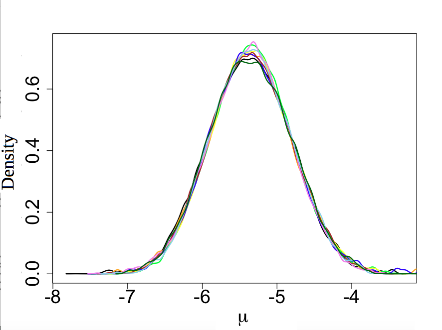
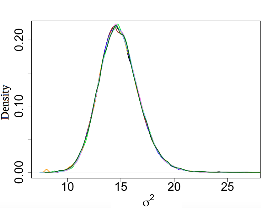
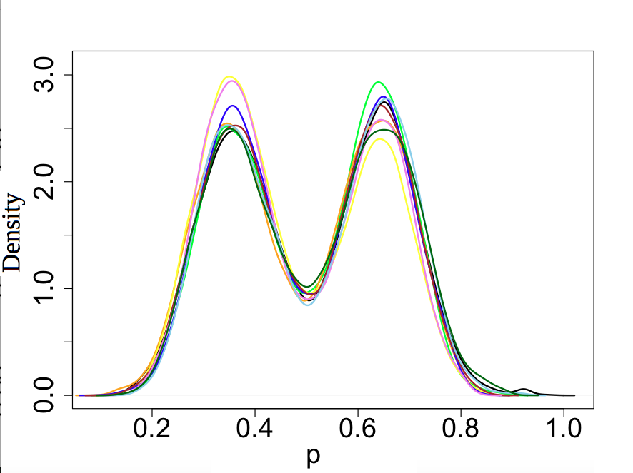
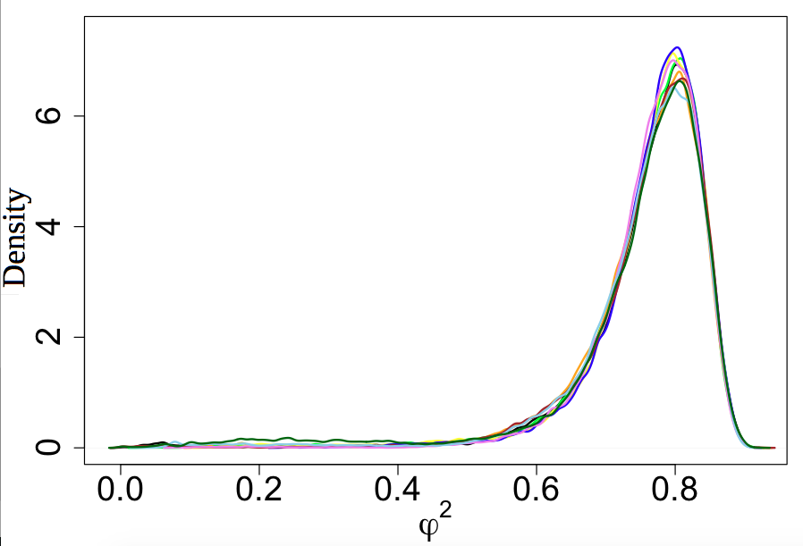
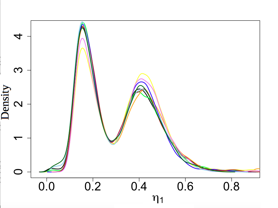
Figure 3: Example 4.1: Kernel estimates of the posterior densities of the parameters $\mu$, $\sigma$, $p$, $\varphi$, $\eta_{i}$, based on $10$ parallel MCMC chains for Proposal 1 and $2\times 10^{5}$ iterations, based on a single simulated sample of size $50$. The true value of $(\mu,\sigma^{2},p,\varphi^{2},\eta_{1},\eta_{2})$ is $(-5.37,15.75,0.65,0.81,0.15,0.41)$.

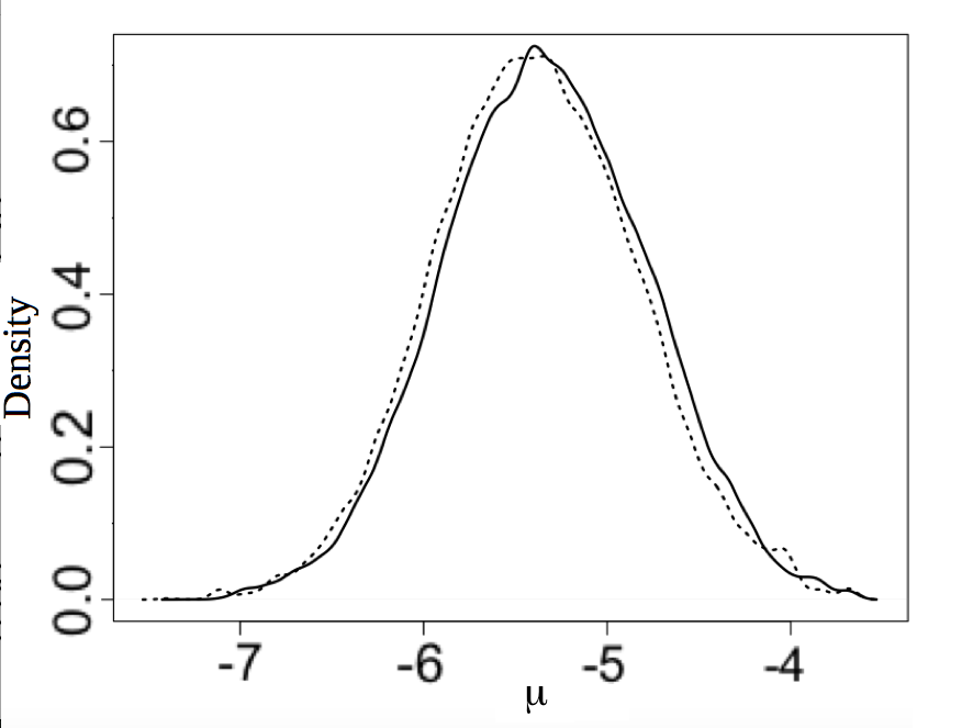
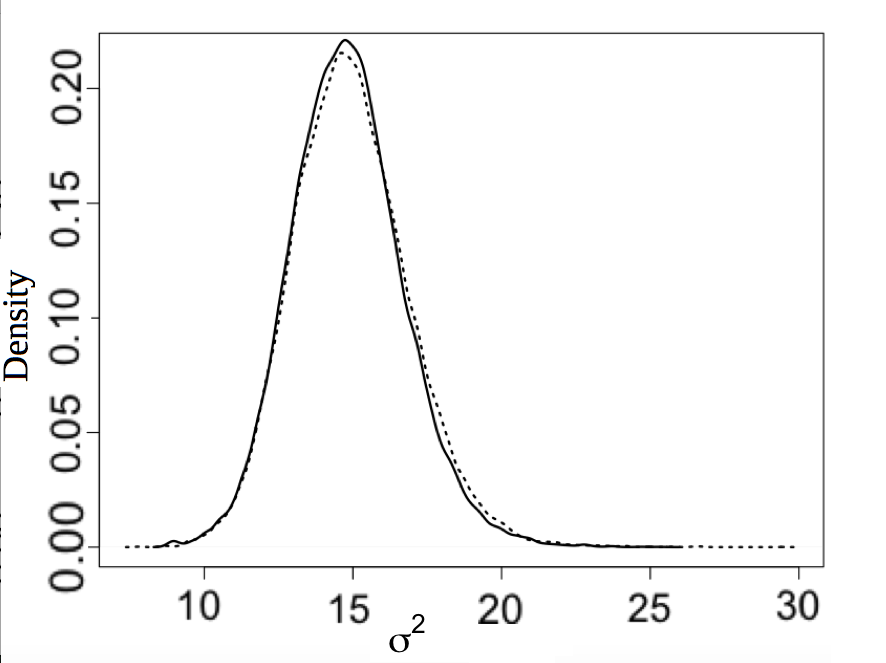
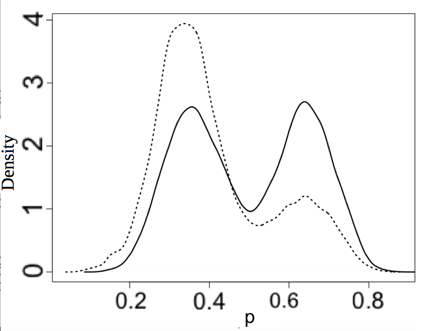
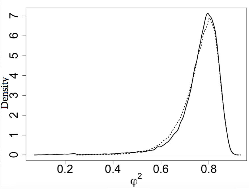
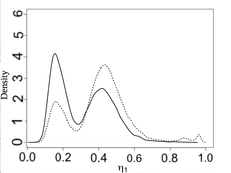
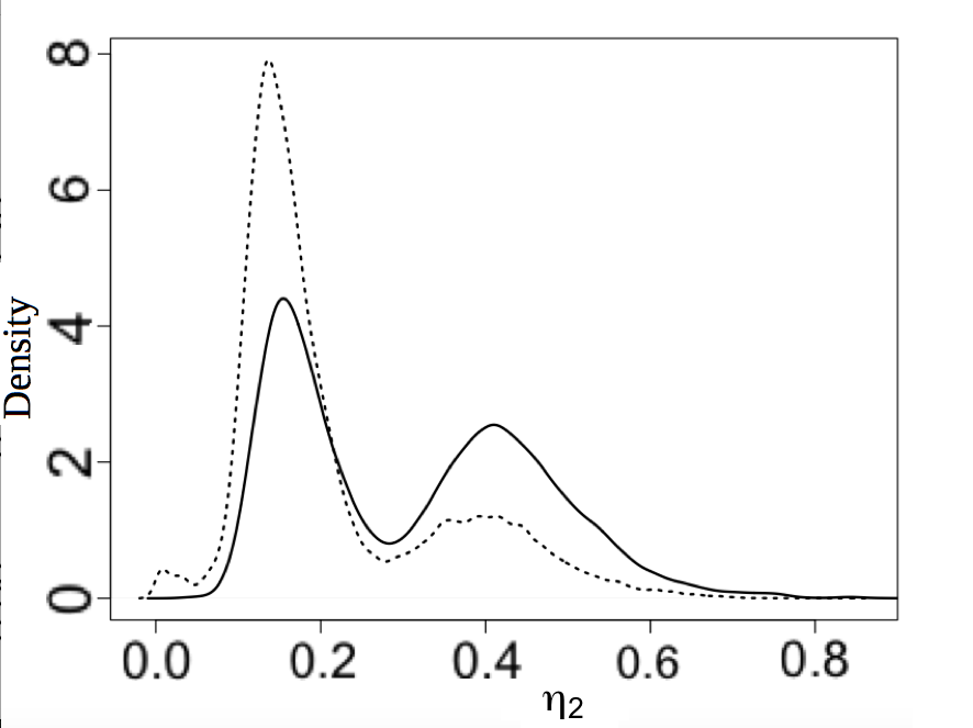
Figure 4: Example 4.1: Comparison between MCMC samples from our algorithm using Proposal 1 (solid line) and Proposal 2 (dashed line), with $90,000$ iterations and the sample of Figure 3. The true value of $(\mu,\sigma^{2},\varphi^{2},\eta_{1},\eta_{2})$ is $(-5.375,15.747,0.813,0.149,0.406)$.

Proposal 1	$ar_{\mu}$	$ar_{\sigma}$	$ar_{p}$	$ar_{\varphi,\eta}$	$\epsilon_{\mu}$	$\epsilon_{p}$	$\epsilon$
	0.40	0.47	0.45	0.24	0.56	77.06	99.94
Proposal 2	$ar_{\mu}$	$ar_{\sigma}$	$ar_{p}$	$ar_{\varphi,\eta}$	$\epsilon_{\mu}$	$\epsilon_{p}$	$\epsilon_{\vartheta}$
	0.38	0.46	0.45	0.27	0.55	0.29	0.35

Table 1: Example 4.1: Acceptance rate ($ar$) and corresponding proposal scale ($\epsilon$) when the adaptive Metropolis-within-Gibbs sampler is used.

4.2 The general Gaussian mixture model

We now consider the general case of estimating a mixture for any $k$ when the variance vector $(\eta_{1}^{2},\ldots,\eta_{k}^{2})$ also has the spherical coordinate system as represented in Section 2.3.2. All algorithms used in this section are publicly available within our R package Ultimixt. The package Ultimixt contains functions that implement adaptive determination of optimal scales and convergence monitoring based on Gelman and Rubin (1992) criterion. In addition, Ultimixt includes functions that summarise the simulations and compute point estimates of each parameter, such as posterior mean and median. It also produces an estimated mixture density in numerical and graphical formats. The output further provides graphical representations of the generated parameter samples.

Example 4.2

The sample is made of 50 simulation from the mixture

$$0.27\mathcal{N}(-4.5,1)+0.4\mathcal{N}(10,1)+0.33\mathcal{N}(3,1)\,.$$

Since this is a Gaussian mixture with the common variance of 1, simulated chains of component-wise mean parameters and weights are good indicators to monitor whether the chain explores all posterior modes. Monitoring the chain for an angle parameter $\varpi$ and $p_{i}$, we illustrate the motivation of sampling $\eta$ and $\varpi$ through two steps in Figure 10, Supplementary Material.

From our simulation experience of the adaptive Metropolis-within-Gibbs algorithm using only a random walk proposal (restrict to Step 2.8), the simulated samples were quite close to the true values; however, the chain visited only one of the posterior modes. This lack of label switching helps us in producing point estimates directly from this MCMC output (Geweke, 2007) but this also shows an incomplete convergence of the MCMC sampler.

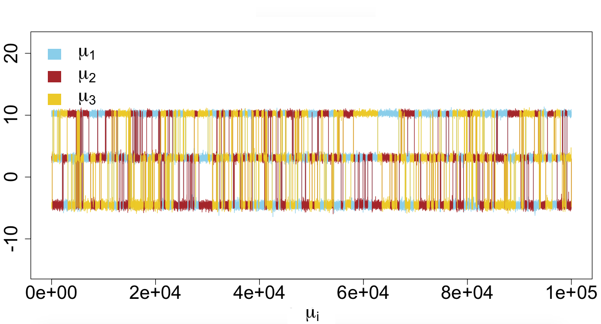
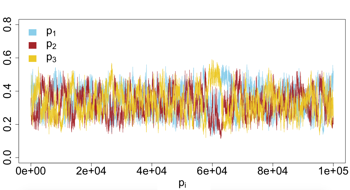
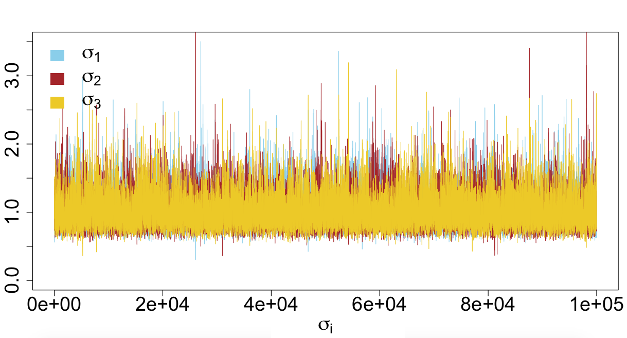
Figure 13: Example 4.2: Traces of $10^{5}$ simulations from the posterior distributions of the component means, standard deviations and weights, involving an additional random walk proposal on $\varpi$.

To help the chain visit all posterior modes, the proposals are restricted to Step 2.4 of the Metropolis-within-Gibbs algorithm, namely using only a uniform distribution $\mathcal{U}[0,2\pi]$. The MCMC samples on the $p_{i}$’s are both well-mixed and exhibit strong exchangeability (see Figure 12 in the Supplementary Material). However, the corresponding acceptance rate is quite low at $0.051$. To increase this rate, the random walk proposal of Step 2.8 on $\varpi$, namely $\mathcal{U}(\varpi^{(t)}-\epsilon_{\varpi},\varpi^{(t)}+\epsilon_{\varpi})$, is added and this clearly improves performances, with acceptance rates all close to $0.234$ and $0.44$. Almost perfect label switching occurs in this case (see Figure 13 in the Supplementary Material). Hence posterior samples for $\eta$’s and $\varpi$’s are generated using an independent proposal plus a random walk proposal in our adaptive Metropolis-within-Gibbs algorithm.

The simulated chains are almost indistinguishable component-wise, due to label switching. As described in Section 3.3, we relabelled the MCMC chains using both (a) a k-means clustering algorithm and (b) a removal of label switching by permutations, as presented in Section 3.3. Point estimates of the relabelled chain are shown in Table 2 and the marginal posterior distributions of component-wise mean and standard deviation are shown in Figure 5. Bayesian estimations computed by both methods are almost identical and all parameters of the mixture distribution are accurately estimated.

Figure 5: Example 4.2: Estimated marginal posterior densities of component means and standard deviations, based on $10^{5}$ MCMC iterations.

k-means clustering Relabelled using MAP $\varpi$ $\xi_{1}$ $\xi_{2}$ $\varpi$ $\xi_{1}$ $\xi_{2}$ Median 3.54 0.97 0.73 3.32 0.94 0.83 Mean 3.53 0.98 0.72 3.45 0.94 0.82 $p_{1}$ $p_{2}$ $p_{3}$ $p_{1}$ $p_{2}$ $p_{3}$ Median 0.40 0.27 0.33 0.41 0.27 0.33 Mean 0.41 0.27 0.33 0.41 0.27 0.33 $\mu_{1}$ $\mu_{2}$ $\mu_{3}$ $\mu_{1}$ $\mu_{2}$ $\mu_{3}$ Median 10.27 -4.55 3.11 10.27 -4.55 3.11 Mean 10.27 -4.54 3.12 10.26 -4.45 3.11 $\sigma_{1}$ $\sigma_{2}$ $\sigma_{3}$ $\sigma_{1}$ $\sigma_{2}$ $\sigma_{3}$ Median 0.93 1.04 1.01 0.93 1.04 1.03 Mean 0.95 1.08 1.05 0.95 1.07 1.05

Global parameters $\mu$ $\sigma$ $\varphi$ Median 3.98 6.03 0.98 Mean 3.98 6.02 0.99 Proposal scales $\epsilon_{\mu}$ $\epsilon_{\sigma}$ $\epsilon_{p}$ $\epsilon_{\varphi}$ $\epsilon_{\varpi}$ $\epsilon_{\xi}$ 0.33 0.06 190 160 0.09 0.39 Acceptance rates $ar_{\mu}$ $ar_{\sigma}$ $ar_{p}$ $ar_{\varphi}$ $ar_{\varpi}$ $ar_{\xi}$ 0.22 0.34 0.23 0.43 0.42 0.22

Table 2: Example 4.2: Point estimators of the parameters of a mixture of 3 components, proposal scales and corresponding acceptance rates.

Example 4.3

Computer aid tomography (CT) scanning is frequently used in animal science to study the tissue composition of an animal. Figure 6 (a) shows the CT scan image of the cross-section of pork carcass in 256 grey-scale units. Different tissue types produce different intensity-level observations on the CT scan. Pixels attributed to fat tend to have grey scale readings 0-100, muscle 101-220, and bone 221-256. Thompson and Kinghorn (1992), Lee (2009) and McGrory (2013) modelled the composition of the three tissues of a pig carcass using Gaussian mixture models and a model with six components was favoured. In this paper, a random subset of 2000 observations from the original data, made of 36326 observations, is used and estimation of the mixture model is compared to estimates based on the Gibbs sampler of bayesm by Rossi and McCulloch (2010) and on the EM algorithms of mixtools by Benaglia et al. (2009). The data-dependent priors of bayesm on the standard parameters are

$$\mu_{i}\sim N(\bar{\mu},10\sigma_{i})\,,\quad\sigma_{i}^{2}\sim\text{IG}(\nu,3)\quad\text{and}\quad(p_{1},\ldots,p_{k})\sim\mathcal{D}ir(\alpha_{0},\ldots,\alpha_{0})$$

where $\text{IG}(\nu,3)$ is the Inverse-Gamma distribution with scale parameter 3 and degrees of freedom $\nu$. The hyperparameters $\bar{\mu}$ and $\nu$ are derived from the data. Marginal prior distributions of standard parameters using either our double uniform prior (Section 2.3.2) or priors obtained by bayesm are compared graphically in Figure 7. While the priors for $\mu_{i}$ and $\sigma_{i}$ yielded by bayesm do not vary with $k$, our marginal posteriors get more skewed toward $0$ with $k$ but has a longer tail to provide flexible supports for component-wise location and scale parameters. We stress that we fixed the global mean and variance to 0 and 1 here, implying that the outcome will be more variable when the Jeffrey prior is called.

Figure 6: CT image data and the analysis result: (a) The CT image of a cross-section from a pork carcass in grey-scale units. The right bar describes the grey-scale, 0-256. (b) Representation of last 500 MCMC iterations as mixture densities with the overlaid average curve for $k=6$ components (dark line) (c) Comparison between the mixture density estimates obtained by Ultimixt, mixtools and bayesm (d) Mixture model overlapping with distributions of each components: Two violet, brown and blue lines are distributions representing fat tissue, muscle and bone, respectively.

Figure 7: CT image data : Density estimate of 20,000 draws of $\mu_{i},\sigma_{i}$ and $p_{i}$ ($i=1,\ldots,k$) from the prior by bayesm (red lines) and our double uniform prior (black lines) assuming a global mean of 0 and variance of 1 when $k=4$ (first row) and $k=6$ (second row). For the prior by bayesm hyperparameters $\alpha_{0}=5$, $\bar{\mu}=0$ and $\nu=3$ are obtained using bayesm.

Following the analysis of this data by McGrory (2013), a mixture model of six Gaussian components is considered. The resulting means, medians and $95\%$ credible intervals of the parameters of the mixture components are displayed in Table 3, Supplementary Material, along with estimates based on the Gibbs sampler of bayesm (Rossi and McCulloch, 2010) and on the EM algorithms of mixtools (Benaglia et al., 2009), with our approach being produced by Ultimixt (Kamary and Lee, 2017). The MCMC sample from Ultimixt is again summarised by both $k$-means clustering and post-MCMC relabelling using the MAP estimates. As can be seen from Figure 6 (with exact values in Table 3 from the Supplementary Material), the estimates from the three packages Ultimixt, mixtools and bayesm are relatively similar and tissue composition similar to the findings of McGrory (2013) is observed. Figure 6 (d) shows how the composition of tissues is modelled by six Gaussian components which can be interpreted as follows: two components correspond to fat (33%), two to muscle (59%), one to bone (4%) and the remaining component models the mixed tissue of muscle and bone (4%). Among the six components, the biggest component has the weight of $34\%$ and corresponds to muscle. In the intended application, this is the quantity of interest: the higher this percentage, the higher the meat quality of the animal.

4.3 Poisson mixtures

The following example demonstrates how a weakly informative prior for a Poisson mixture is associated with a MCMC algorithm. Under the constraint, $\sum^{k}_{i=1}\gamma_{i}=1$, the Dirichlet prior with the common parameter is used on local parameters $\gamma_{i}$. Any other vague proper prior on this compact space is also suitable.

Example 4.4

The following two Poisson mixture models are considered for various sample sizes, from $50$ to $10^{4}$.

• Model 1: $0.6\mathcal{P}(1)+0.4\mathcal{P}(5)$

• Model 2: $0.3\mathcal{P}(1)+0.4\mathcal{P}(5)+0.3\mathcal{P}(10)$

Figures 8 and 9 display the performances of the Metropolis-within-Gibbs sampler (see also Figure 11 in Supplementary Material). The convergence of the resulting sequence of estimates to the true values is illustrated by the figures as the number of data points increases. While label switching occurs with our prior modelling, as shown in both Figures 8 and 9, the point estimate of each parameter subjected to label switching (component weights and means) can be computed by relabelling the MCMC draws. We then derive point estimates by clustering over the parameter space, using k-mean clustering, resulting in close agreement with the true values.

Figure 8: Mixture of two Poisson distributions 4.4: Comparison between the empirical densities of $5\,10^{4}$ MCMC simulations of (a) the global mean, (b) the weight and (c)-(d) component means. True values are indicated by dashed lines. The different colors in all graphs correspond to the different sample sizes indicated in (a).

Figure 9: Mixture of three Poisson distributions: Comparison between the empirical densities of $5\,10^{4}$ MCMC simulations of (a) the global mean, (b) the component mean $\lambda_{1}$ and weights for two samples of size (c) $n=200$ and (d) $n=10^{4}$. True values are indicated by dashed lines. The different colors in all graphs correspond to the different sample sizes indicated in (a). total number of MCMC iterations is $5\,10^{4}$ with a burn-in of $10^{3}$ iterations.

5 Conclusion

We have introduced a novel parametrisation for location-scale mixture models. By expressing the parameters in terms of the global mean and global variance of the mixture of interest, it has been shown that the remaining parameters vary within a compact set. This reparameterisation makes the use of a well-defined uniform prior possible for these parameters (as well as any proper prior) and we established that an improper prior reproducing the Jeffreys prior on location-scale parameters induces a proper posterior distribution for a minimal sample size. We illustrated the implications of this new prior modelling and of the resulting MCMC algorithms on some standard distributions, namely mixtures of Gaussian, Poisson and exponential distributions and their compound extensions. While the notion of a non-informative or objective prior is mostly open to interpretations and somehow controversial, we argue we have defined in this paper what can be considered as the first reference prior for mixture models. We have shown further that relatively standard simulation algorithms are able to handle these new parametrisations, as exhibited by our Ultimixt R package, and that they can manage the computing issues connected with label switching.

While the extension to non-Gaussian cases with location-scale features is shown here to be conceptually straightforward, considering this reparameterisation in higher dimensions is delicate when made in terms of the covariance matrices. Indeed, even though we can easily set the variance matrix of the mixture model as a reference parameter, reparameterising the component variance matrices against this reference matrix and devising manageable priors remains an open problem that we are currently exploring.

Supplementary material

Appendix A Proof of Lemma 1

The population mean is given by

$$\mathbb{E}_{\boldsymbol{\theta},\mathbf{p}}[X]=\sum_{i=1}^{k}p_{i}\mathbb{E}_{f(\cdot|\theta_{i})}[X]=\sum_{i=1}^{k}p_{i}\mu_{i}$$

where $\mathbb{E}_{f(\cdot|\theta_{i})}[X]$ is the expected value component $i$. Similarly, the population variance is given by

$${\mathrm{var}}_{\boldsymbol{\theta},\mathbf{p}}(X)=\sum^{k}_{i=1}p_{i}\mathbb{E}_{f(\cdot|\theta_{i})}[X^{2}]-\mathbb{E}_{\boldsymbol{\theta},\mathbf{p}}[X]^{2}=\sum_{i=1}^{k}p_{i}(\sigma_{i}^{2}+\mu_{i}^{2})-\mathbb{E}_{\boldsymbol{\theta},\mathbf{p}}[X]^{2}\,,$$

which concludes the proof.

Appendix B Proof of Lemma 2

The result is a trivial consequence of Lemma 1. The population mean is

$$\mathbb{E}_{\boldsymbol{\theta},\mathbf{p}}[X]=\sum_{i=1}^{k}p_{i}\mu_{i}=\sum_{i=1}^{k}p_{i}(\mu+\sigma\alpha_{i})=\mu+\sigma\sum_{i=1}^{k}p_{i}\alpha_{i}$$

and the first constraint follows. The population variance is

$$\begin{array}[]{c c l}{\mathrm{var}}_{\boldsymbol{\theta},\mathbf{p}}(X)&=&\displaystyle\sum_{i=1}^{k}p_{i}\sigma_{i}^{2}+\sum_{i=1}^{k}p_{i}(\mu_{i}^{2}-\mathbb{E}_{\boldsymbol{\theta},\mathbf{p}}[X]^{2})\\ &=&\displaystyle\sum_{i=1}^{k}p_{i}\sigma^{2}\tau_{i}^{2}+\sum_{i=1}^{k}p_{i}(\mu^{2}+2\sigma\mu\alpha_{i}+\sigma^{2}\alpha_{i}^{2}-\mu^{2})\\ &=&\displaystyle\sum_{i=1}^{k}p_{i}\sigma^{2}\tau_{i}^{2}+\sum_{i=1}^{k}p_{i}\sigma^{2}\alpha_{i}^{2}\end{array}$$

The last equation simplifies to the second constraint above.

Appendix C Proof of Theorem 1

When $n=1$, it is easy to show that the posterior is not proper. The marginal likelihood is then

$$\begin{array}[]{c c l}M_{k}(x_{1})&=&\displaystyle\sum^{k}_{i=1}\int p_{i}f(x_{1}|\mu+\sigma\alpha_{i},\sigma^{2}\tau_{i}^{2})\pi(\mu,\sigma,\mathbf{p},\boldsymbol{\alpha},\boldsymbol{\tau})\,\text{d}(\mu,\sigma,\mathbf{p},\boldsymbol{\alpha},\boldsymbol{\tau})\\ &=&\displaystyle\sum^{k}_{i=1}\int\left\{\int\dfrac{p_{i}}{\sqrt{2\pi}\sigma^{2}\tau_{i}}\exp\left(\dfrac{-(x_{1}-\mu-\sigma\alpha_{i})^{2}}{2\tau_{i}^{2}\sigma^{2}}\right)\,\text{d}(\mu,\sigma)\right\}\pi(\mathbf{p},\boldsymbol{\alpha},\boldsymbol{\tau})\,\text{d}(\mathbf{p},\boldsymbol{\alpha},\boldsymbol{\tau})\\ &=&\displaystyle\sum^{k}_{i=1}\int\left\{\int_{0}^{\infty}\dfrac{p_{i}}{\sigma}\,\text{d}\sigma\right\}\pi(\mathbf{p},\boldsymbol{\alpha},\boldsymbol{\tau})\,\text{d}(\mathbf{p},\boldsymbol{\alpha},\boldsymbol{\tau})\\ \end{array}$$

The integral against $\sigma$ is then not defined.

For two data-points, $x_{1},x_{2}\sim\sum^{k}_{i=1}p_{i}f(\mu+\sigma\alpha_{i},\sigma^{2}\tau_{i}^{2})$, the associated marginal likelihood is

$$\begin{array}[]{c c l}M_{k}(x_{1},x_{2})&=&\displaystyle\int\prod^{2}_{j=1}\left\{\sum^{k}_{i=1}p_{i}f(x_{j}|\mu+\sigma\alpha_{i},\sigma^{2}\tau_{i}^{2})\right\}\pi(\mu,\sigma,\mathbf{p},\boldsymbol{\alpha},\boldsymbol{\tau})\,\text{d}(\mu,\sigma,\mathbf{p},\boldsymbol{\alpha},\boldsymbol{\tau})\\ &=&\displaystyle\sum^{k}_{i=1}\displaystyle\sum^{k}_{j=1}\displaystyle\int p_{i}p_{j}f(x_{1}|\mu+\sigma\alpha_{i},\sigma^{2}\tau_{i}^{2})f(x_{2}|\mu+\sigma\alpha_{j},\sigma^{2}\tau_{j}^{2})\pi(\mu,\sigma,\mathbf{p},\boldsymbol{\alpha},\boldsymbol{\tau})\,\text{d}(\mu,\sigma,\mathbf{p},\boldsymbol{\alpha},\boldsymbol{\tau})~{}.\end{array}$$

If all those $k^{2}$ integrals are proper, the posterior distribution is proper. An arbitrary integral $(1\leq i,j\leq k)$ in this sum leads to

$$\begin{array}[]{l l}\displaystyle\int&p_{i}p_{j}f(x_{1}|\mu+\sigma\alpha_{i},\sigma^{2}\tau_{i}^{2})f(x_{2}|\mu+\sigma\alpha_{j},\sigma^{2}\tau_{j}^{2})\pi(\mu,\sigma,\mathbf{p},\boldsymbol{\alpha},\boldsymbol{\tau})\,\text{d}(\mu,\sigma,\mathbf{p},\boldsymbol{\alpha},\boldsymbol{\tau})\\ =&\displaystyle\int\Bigg{\{}\int\dfrac{p_{i}p_{j}}{2\pi\sigma^{3}\tau_{i}\tau_{j}}\exp\Bigg{[}\dfrac{-(x_{1}-\mu-\sigma\alpha_{i})^{2}}{2\tau_{i}^{2}\sigma^{2}}+\dfrac{-(x_{2}-\mu-\sigma\alpha_{j})^{2}}{2\tau_{j}^{2}\sigma^{2}}\Bigg{]}\text{d}(\mu,\sigma)\Bigg{\}}\pi(\mathbf{p},\boldsymbol{\alpha},\boldsymbol{\tau})\,\text{d}(\mathbf{p},\boldsymbol{\alpha},\boldsymbol{\tau})\\ =&\displaystyle\int\Bigg{\{}\int_{0}^{\infty}\dfrac{p_{i}p_{j}}{\sqrt{2\pi}\sigma^{2}\sqrt{\tau^{2}_{i}+\tau^{2}_{j}}}\exp\Bigg{[}\dfrac{-1}{2(\tau_{i}^{2}+\tau_{j}^{2})}\Bigg{(}\dfrac{1}{\sigma^{2}}(x_{1}-x_{2})^{2}+\dfrac{2}{\sigma}(x_{1}-x_{2})(\alpha_{i}-\alpha_{j})\\ &\qquad+(\alpha_{i}-\alpha_{j})^{2}\Bigg{)}\Bigg{]}\,\text{d}\sigma\Bigg{\}}\pi(\mathbf{p},\boldsymbol{\alpha},\boldsymbol{\tau})\,\text{d}(\sigma,\mathbf{p},\boldsymbol{\alpha},\boldsymbol{\tau})\,.\end{array}$$

Substituting $\sigma=1/z$, the above is integrated with respect to $z$, leading to

$$\begin{array}[]{l l}\displaystyle\int&\Bigg{\{}\displaystyle\int_{0}^{\infty}\dfrac{p_{i}p_{j}}{\sqrt{2\pi}\sqrt{\tau^{2}_{i}+\tau^{2}_{j}}}\exp\Bigg{(}\dfrac{-1}{2(\tau_{i}^{2}+\tau_{j}^{2})}\Bigg{(}z^{2}(x_{1}-x_{2})^{2}+2z(x_{1}-x_{2})(\alpha_{i}-\alpha_{j})\\ &\qquad+(\alpha_{i}-\alpha_{j})^{2}\Bigg{)}\Bigg{)}\,\text{d}z\Bigg{\}}\pi(\mathbf{p},\boldsymbol{\alpha},\boldsymbol{\tau})\,\text{d}(\mathbf{p},\boldsymbol{\alpha},\boldsymbol{\tau})\\ =&\displaystyle\int\Bigg{\{}\displaystyle\int_{0}^{\infty}\dfrac{p_{i}p_{j}}{\sqrt{2\pi}\sqrt{\tau^{2}_{i}+\tau^{2}_{j}}}\exp\Bigg{(}\dfrac{-(x_{1}-x_{2})^{2}}{2(\tau_{i}^{2}+\tau_{j}^{2})}\Big{(}z+\dfrac{\alpha_{i}-\alpha_{j}}{x_{1}-x_{2}}\Big{)}^{2}\Bigg{)}\,\text{d}z\Bigg{\}}\pi(\mathbf{p},\boldsymbol{\alpha},\boldsymbol{\tau})\,\text{d}(\mathbf{p},\boldsymbol{\alpha},\boldsymbol{\tau})\\ =&\displaystyle\int\frac{p_{i}p_{j}}{|x_{1}-x_{2}|}\Phi\left(-\dfrac{\alpha_{i}-\alpha_{j}}{x_{1}-x_{2}}\dfrac{|x_{1}-x_{2}|}{\sqrt{\tau_{i}^{2}+\tau_{j}^{2}}}\right)\pi(\mathbf{p},\boldsymbol{\alpha},\boldsymbol{\tau})~{}\text{d}(\mathbf{p},\boldsymbol{\alpha},\boldsymbol{\tau})\,,\end{array}$$

where $\Phi$ is the cumulative distribution function of the standardised Normal distribution. Given that the prior is proper on all remaining parameters of the mixture, it follows that the integrand is bounded by $1/|x_{1}-x_{2}|$, and so it integrates against the remaining components of $\boldsymbol{\theta}$. Now, consider the case $n\geq 3$. Since the posterior $\pi(\boldsymbol{\theta}|x_{1},x_{2})$ is proper, it constitutes a proper prior when considering only the observations $x_{3},\ldots,x_{n}$. Therefore, the posterior is almost everywhere proper.

Appendix D Proof of Theorem 2

Considering one single positive observation $x_{1}$, the marginal likelihood is

$$M_{k}(x_{1}) =\sum_{i=1}^{k}\int p_{i}f(x_{1}|\lambda\gamma_{i}/p_{i})\pi(\lambda,\boldsymbol{\gamma},\boldsymbol{p})d(\lambda,\boldsymbol{\gamma},\boldsymbol{p})$$

$$=\sum_{i=1}^{k}\int\left(\int_{0}^{\infty}p_{i}\exp(-\lambda\gamma_{i}/p_{i})(\lambda\gamma_{i}/p_{i})^{x_{1}}/x_{1}!\pi(\lambda)d\lambda\right)\pi(\boldsymbol{\gamma},\boldsymbol{p})d(\boldsymbol{\gamma},\boldsymbol{p})$$

$$=\sum_{i=1}^{k}\int\left(p_{i}(\gamma_{i}/p_{i})^{x_{1}}/{x_{1}}!\int_{0}^{\infty}\exp(-\lambda\gamma_{i}/p_{i})\lambda^{x_{1}-1}d\lambda\right)\pi(\boldsymbol{\gamma},\boldsymbol{p})d(\boldsymbol{\gamma},\boldsymbol{p})$$

$$=\sum_{i=1}^{k}\int\left(p_{i}/x_{1}\right)\pi(\boldsymbol{\gamma},\boldsymbol{p})d(\boldsymbol{\gamma},\boldsymbol{p})$$

Since the prior is proper on all remaining parameters of the mixture, the integrals in the above sum are all finite. The posterior $\pi(\lambda,\boldsymbol{\gamma},\boldsymbol{p}|x_{1})$ is therefore proper and it constitutes a proper prior when considering further observations $x_{2},\ldots,x_{n}$. Therefore, the resulting posterior for the sample $(x_{1},\ldots,x_{n})$ is proper.

Appendix E Proof of Theorem 3

Considering one single observation $x_{1}$, the marginal likelihood is

$$M_{k}(x_{1}) =\sum_{i=1}^{k}\int p_{i}f(x_{1}|p_{i}/\lambda\gamma_{i})\pi(\lambda,\boldsymbol{\gamma},\boldsymbol{p})d(\lambda,\boldsymbol{\gamma},\boldsymbol{p})$$

$$=\sum_{i=1}^{k}\int\left(\int_{0}^{\infty}p_{i}\exp(-\nicefrac{{p_{i}x}}{{\lambda\gamma_{i}}})\nicefrac{{p_{i}}}{{\lambda\gamma_{i}}}\pi(\lambda)d\lambda\right)\pi(\boldsymbol{\gamma},\boldsymbol{p})\text{d}(\boldsymbol{\gamma},\boldsymbol{p})$$

$$=\sum_{i=1}^{k}\int p_{i}\int_{0}^{\infty}\nicefrac{{p_{i}}}{{\lambda\gamma_{i}}}\exp(-\lambda\gamma_{i}x_{1}/p_{i})\text{d}\lambda\pi(\boldsymbol{\gamma},\boldsymbol{p})\text{d}(\boldsymbol{\gamma},\boldsymbol{p})$$

$$=\sum_{i=1}^{k}\int\left(p_{i}/x_{1}\right)\pi(\boldsymbol{\gamma},\boldsymbol{p})\text{d}(\boldsymbol{\gamma},\boldsymbol{p})\,.$$

Since the prior is proper on all remaining parameters of the mixture, the integrals in the above sum are all finite. The posterior $\pi(\lambda,\boldsymbol{\gamma},\boldsymbol{p}|x_{1})$ is therefore proper and it constitutes a proper prior when considering further observations $x_{2},\ldots,x_{n}$. Therefore, the resulting posterior for the sample $(x_{1},\ldots,x_{n})$ is proper.

Appendix F Pseudo-code representations of the MCMC algorithms for the Normal and Poisson cases

Metropolis-within-Gibbs algorithm for a reparameterised Gaussian mixture 1 Generate initial values $(\mu^{(0)},\sigma^{(0)},\mathbf{p}^{(0)},\varphi^{(0)},\xi_{1}^{(0)},\ldots,\xi^{(0)}_{k-1},\varpi^{(0)}_{1},\ldots,\varpi^{(0)}_{k-2})$. 2 For $t=1,\ldots,T$, the update of $(\mu^{(t)},\sigma^{(t)},\mathbf{p}^{(t)},\varphi^{(t)},\xi_{1}^{(t)},\ldots,\xi^{(t)}_{k-1},\varpi^{(t)}_{1},\ldots,\varpi^{(t)}_{k-2})$
is as follows; 2.1 Generate a proposal $\mu^{\prime}\sim\mathcal{N}(\mu^{(t-1)},\epsilon_{\mu})$ and update $\mu^{(t)}$ against $\pi(\cdot|\mathbf{x},\sigma^{(t-1)},\mathbf{p}^{(t-1)},\varphi^{(t-1)},\boldsymbol{\xi}^{(t-1)},\boldsymbol{\varpi}^{(t-1)})$. 2.2 Generate a proposal $\log(\sigma)^{\prime}\sim\mathcal{N}(\log(\sigma^{(t-1)}),\epsilon_{\sigma})$ and update $\sigma^{(t)}$ against $\pi(\cdot|\mathbf{x},\mu^{(t)},\mathbf{p}^{(t-1)},\varphi^{(t-1)},\boldsymbol{\xi}^{(t-1)},\boldsymbol{\varpi}^{(t-1)})$. 2.3 Generate proposals $\xi^{\prime}_{i}\sim\mathcal{U}[0,\pi/2]$, $i=1,\cdots,k-1$, and update $(\xi^{(t)}_{1},\ldots,\xi^{(t)}_{k-1})$ against $\pi(\cdot|\mathbf{x},\mu^{(t)},\sigma^{(t)},\mathbf{p}^{(t-1)},\varphi^{(t-1)},\boldsymbol{\varpi}^{(t-1)})$. 2.4 Generate proposals $\varpi^{\prime}_{i}\sim\mathcal{U}[0,\pi]$, $i=1,\cdots,k-3$, and $\varpi^{\prime}_{k-2}\sim\mathcal{U}[0,2\pi]$. Update $(\varpi^{(t)}_{1},\ldots,\varpi^{(t)}_{k-2})$ against $\pi(\cdot|\mathbf{x},\mu^{(t)},\sigma^{(t)},\mathbf{p}^{(t-1)},\varphi^{(t-1)},\boldsymbol{\xi}^{(t)})$. 2.5 Generate a proposal $(\varphi^{2})^{\prime}\sim\mathcal{B}eta((\varphi^{2})^{(t)}\epsilon_{\varphi}+1,(1-(\varphi^{2})^{(t)})\epsilon_{\varphi}+1)$ and update $\varphi^{(t)}$ against $\pi(\cdot|\mathbf{x},\mu^{(t)},\sigma^{(t)},\mathbf{p}^{(t-1)},\boldsymbol{\xi}^{(t)},\boldsymbol{\varpi}^{(t)})$. 2.6 Generate a proposal $\mathbf{p}^{\prime}\sim\text{Dir}(p_{1}^{(t-1)}\epsilon_{p}+1,\ldots,p_{k}^{(t-1)}\epsilon_{p}+1)$, and update $\mathbf{p}^{(t)}$ against $\pi(\cdot|\mathbf{x},\mu^{(t)},\sigma^{(t)},\varphi^{(t)},\boldsymbol{\xi}^{(t)},\boldsymbol{\varpi}^{(t)})$. 2.7 Generate proposals $\xi^{\prime}_{i}\sim U[\xi^{(t)}_{i}-\epsilon_{\xi},\xi^{(t)}_{i}+\epsilon_{\xi}]$, $i=1,\cdots,k-1$, and update $(\xi^{(t)}_{1},\ldots,\xi^{(t)}_{k-1})$ against $\pi(\cdot|\mathbf{x},\mu^{(t)},\sigma^{(t)},\mathbf{p}^{(t)},\varphi^{(t)},\boldsymbol{\varpi}^{(t)})$. 2.8 Generate proposals $\varpi^{\prime}_{i}\sim U[\varpi^{(t)}_{i}-\epsilon_{\varpi},\varpi^{(t)}_{i}+\epsilon_{\varpi}]$, $i=1,\cdots,k-2$, and update $(\varpi^{(t)}_{1},\ldots,\varpi^{(t)}_{k-2})$ against $\pi(\cdot|\mathbf{x},\mu^{(t)},\sigma^{(t)},\mathbf{p}^{(t)},\varphi^{(t)},\boldsymbol{\xi}^{(t)})$.

Figure 10: Pseudo-code representation of the Metropolis-within-Gibbs algorithm used in this paper for reparameterisation (ii) of the Gaussian mixture model, based on two sets of spherical coordinates. For simplicity’s sake, we denote $\mathbf{p}^{(t)}=(p_{1}^{(t)},\ldots,p_{k}^{(t)})$, $\mathbf{x}=(x_{1},\ldots,x_{n})$, $\boldsymbol{\xi}^{(t)}=(\xi_{1}^{(t)},\ldots,\xi^{(t)}_{k-1})$ and $\boldsymbol{\varpi}^{(t)}=(\varpi^{(t)}_{1},\ldots,\varpi^{(t)}_{k-2})$.

Metropolis-within-Gibbs algorithm for a reparameterised Poisson mixture 1 Generate initial values $(\lambda^{(0)},\boldsymbol{\gamma}^{(0)},\mathbf{p}^{(0)})$. 2 For $t=1,\ldots,T$, the update of $(\lambda^{(t)},\boldsymbol{\gamma}^{(t)},\mathbf{p}^{(t)})$
is as follows; 2.1 Generate a proposal $\lambda^{\prime}\sim\mathcal{N}(\log(\overline{X}),\epsilon_{\lambda})$ and update $\lambda^{(t)}$ against $\pi(\cdot|\mathbf{x},\boldsymbol{\gamma}^{(t-1)},\mathbf{p}^{(t-1)})$. 2.2 Generate a proposal $\boldsymbol{\gamma}^{\prime}\sim\text{Dir}(\gamma_{1}^{(t-1)}\epsilon_{\gamma}+1,\ldots,\gamma_{k}^{(t-1)}\epsilon_{\gamma}+1)$, and update $\boldsymbol{\gamma}^{(t)}$ against $\pi(\cdot|\mathbf{x},\lambda^{(t)},\mathbf{p}^{(t-1)})$. 2.3 Generate a proposal $\mathbf{p}^{\prime}\sim\text{Dir}(\mathbf{p}_{1}^{(t-1)}\epsilon_{p}+1,\ldots,\mathbf{p}_{k}^{(t-1)}\epsilon_{p}+1)$, and update $\mathbf{p}^{(t)}$ against $\pi(\cdot|\mathbf{x},\lambda^{(t)},\boldsymbol{\gamma}^{(t)})$.

Figure 11: Pseudo-code representation of the Metropolis-within-Gibbs algorithm used to approximate the posterior distribution of the reparameterisation of the Poisson mixture. For $i=1,\ldots,k$, we denote $\boldsymbol{\gamma}=(\gamma_{1},\ldots,\gamma_{k})$, $\mathbf{p}^{(t)}=(p_{1}^{(t)},\ldots,p_{k}^{(t)})$ and $\mathbf{x}=(x_{1},\ldots,x_{n})$. $\overline{X}$ is the empirical mean of the observations.

Appendix G Convergence graphs for Example 4.2

Figure 12: Example 4.2: (Left) Evolution of the sequence $(\varpi^{(t)})$ and (Right) histograms of the simulated weights based on $10^{5}$ iterations of an adaptive Metropolis-within-Gibbs algorithm with independent proposal on $\varpi$.

Appendix H An illustration of the proposal impact on Old Faithful

We analysed the R benchmark Old Faithful dataset, using the 272 observations of eruption times and a mixture model with two components. The empirical mean and variance of the observations are $(3.49,1.30)$.

When using Proposal 1, the optimal scales $\epsilon_{\mu},\epsilon_{p},\epsilon$ after $50,000$ iterations are $0.07,\allowbreak 501.1,\allowbreak 802.19$, respectively. The posterior distributions of the generated samples shown in Figure 14 demonstrate a strong concentration of $(\mu,\sigma^{2})$ near the empirical mean and variance. There is a strong indication that the chain gets trapped into a single mode of the posterior density.

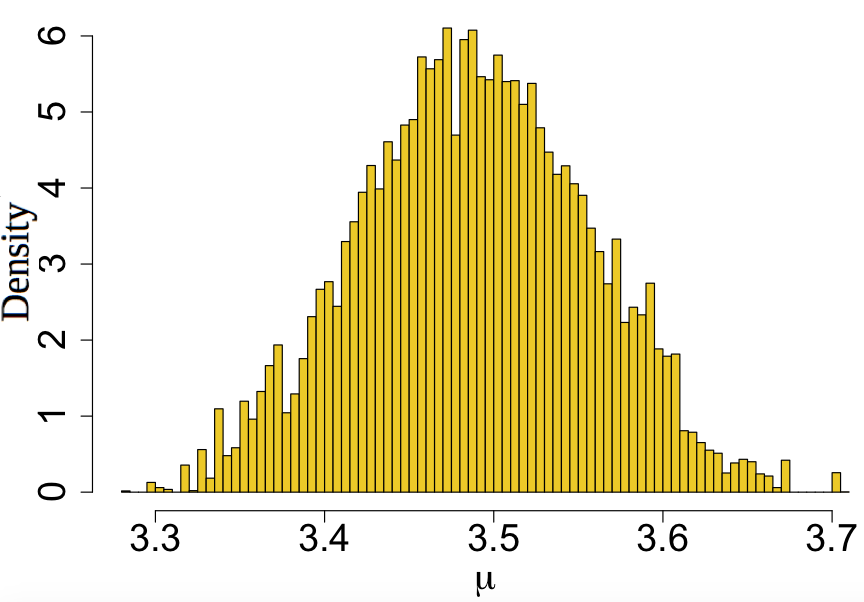
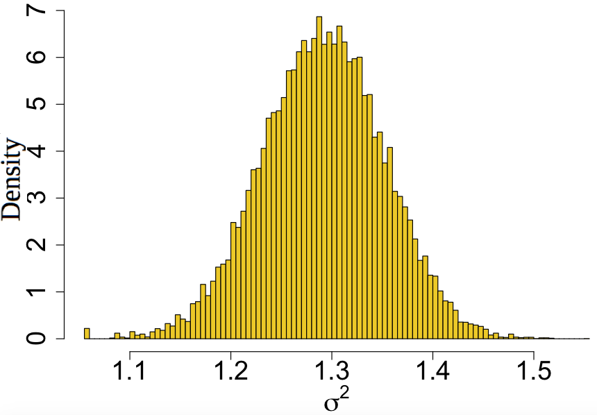
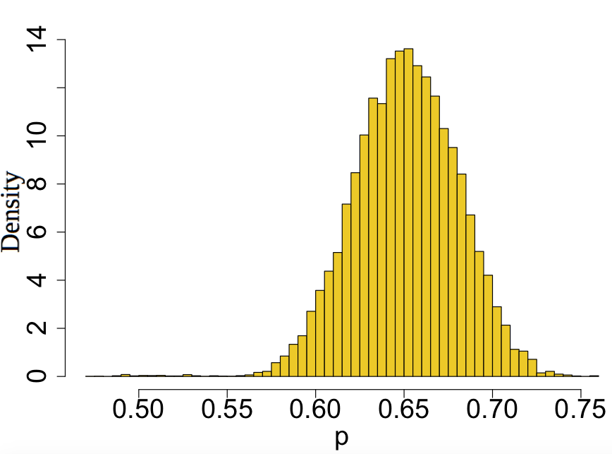
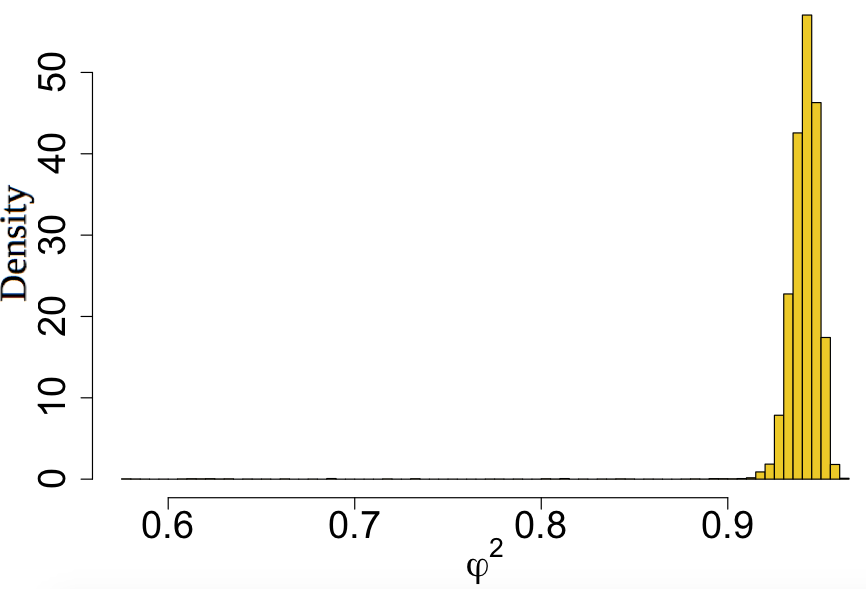
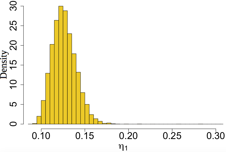
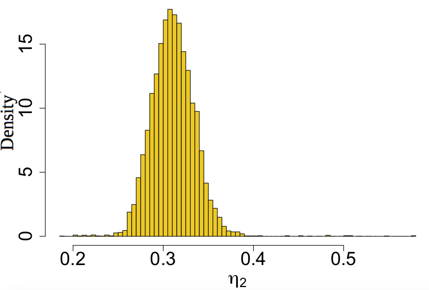
Figure 14: Old Faithful dataset: Posterior distributions of the parameters of a two-component mixture distribution based on $50,000$ MCMC iterations.

Appendix I Values of estimates of the mixture parameters behind the CT dataset

k-means clustering (Ultimixt) $p_{1}$ $p_{2}$ $p_{3}$ $p_{4}$ $p_{5}$ $p_{6}$ Median 0.16 0.17 0.25 0.34 0.04 0.04 Mean 0.16 0.17 0.25 0.34 0.03 0.04 $\mu_{1}$ $\mu_{2}$ $\mu_{3}$ $\mu_{4}$ $\mu_{5}$ $\mu_{6}$ Median 68.75 89.88 121.0 134.6 201.3 244.4 Mean 68.68 89.88 121.1 134.6 203.3 242.2 $\sigma_{1}$ $\sigma_{2}$ $\sigma_{3}$ $\sigma_{4}$ $\sigma_{5}$ $\sigma_{6}$ Median 17.37 9.380 13.66 4.613 23.62 2.055 Mean 17.38 9.388 13.69 4.615 22.72 2.995 Relabelled using MAP (Ultimixt) $p_{1}$ $p_{2}$ $p_{3}$ $p_{4}$ $p_{5}$ $p_{6}$ Median 0.16 0.17 0.25 0.34 0.03 0.04 Mean 0.16 0.17 0.25 0.34 0.03 0.04 2.5% $0.15$ $0.16$ $0.24$ $0.33$ $0.03$ $0.04$ 97.5% 0.17 0.18 0.27 0.36 0.04 0.05 $\mu_{1}$ $\mu_{2}$ $\mu_{3}$ $\mu_{4}$ $\mu_{5}$ $\mu_{6}$ Median 68.71 89.91 121.0 134.6 201.0 244.4 Mean 68.67 89.92 121.1 134.6 201.1 244.3 2.5% 65.89 88.85 120.4 134.2 196.3 243.9 97.5% 71.10 90.82 122.5 135.1 206.3 244.9 $\sigma_{1}$ $\sigma_{2}$ $\sigma_{3}$ $\sigma_{4}$ $\sigma_{5}$ $\sigma_{6}$ Median 17.37 9.386 13.62 4.615 23.62 2.054 Mean 17.38 9.391 13.71 4.621 23.66 2.047 2.5% 16.43 8.673 12.83 4.370 21.89 1.822 97.5% 18.38 10.12 14.80 4.871 25.67 2.220

Gibbs sampler (bayesm) $p_{1}$ $p_{2}$ $p_{3}$ $p_{4}$ $p_{5}$ $p_{6}$ Mean 0.17 0.18 0.21 0.36 0.04 0.04 $\mu_{1}$ $\mu_{2}$ $\mu_{3}$ $\mu_{4}$ $\mu_{5}$ $\mu_{6}$ Mean 69.74 88.99 119.94 134.48 196.69 243.94 $\sigma_{1}$ $\sigma_{2}$ $\sigma_{3}$ $\sigma_{4}$ $\sigma_{5}$ $\sigma_{6}$ Mean 18.44 8.048 10.85 4.956 24.08 3.808 EM estimate (mixtools) $p_{1}$ $p_{2}$ $p_{3}$ $p_{4}$ $p_{5}$ $p_{6}$ 0.15 0.18 0.27 0.33 0.04 0.04 $\mu_{1}$ $\mu_{2}$ $\mu_{3}$ $\mu_{4}$ $\mu_{5}$ $\mu_{6}$ 67.62 88.57 121.9 134.6 203.2 244.5 $\sigma_{1}$ $\sigma_{2}$ $\sigma_{3}$ $\sigma_{4}$ $\sigma_{5}$ $\sigma_{6}$ 17.42 7.818 13.84 4.579 23.27 1.841

Table 3: CT image dataset: Estimates of the parameters of a mixture of 6 components.

Appendix J R codes

File “allcodes.tar.gz” contains all R codes used to produce the examples processed in the paper (this is a GNU zipped tar file). In addition, the R package Ultimixt is deposited on CRAN and contains R functions to estimate univariate mixture models from one of the three families studied in this paper.

References

- Andrews and Mallows (1974) Andrews, D. F. and Mallows, C. L. (1974). Scale mixtures of normal distributions. J. Royal Statist. Society Series B, 36 99–102.
- Benaglia et al. (2009) Benaglia, T., Chauveau, D., Hunter, D. and Young, D. (2009). mixtools: An R package for analyzing finite mixture models. J. Statistical Software, 32 1–29.
- Berkhof et al. (2003) Berkhof, J., van Mechelen, I. and Gelman, A. (2003). A Bayesian approach to the selection and testing of mixture models. Statistica Sinica, 13 423–442.
- Berger (2004) Berger, J. (2004). The case for objective Bayesian analysis. Bayesian Analysis, 1 1–17.
- Berger et al. (2009) Berger, J., Bernardo, J. and Sun, D. (2009). Natural induction: An objective Bayesian approach. Rev. R. Acad. Cien. Serie A. Mat., 103 125–135.
- Bernardo and Giròn (1988) Bernardo, J. and Giròn, F. (1988). A Bayesian analysis of simple mixture problems. In Bayesian Statistics 3 (J. Bernardo, M. DeGroot, D. Lindley and A. Smith, eds.). Oxford University Press, Oxford, 67–78.
- Celeux et al. (2000) Celeux, G., Hurn, M. and Robert, C. (2000). Computational and inferential difficulties with mixture posterior distributions. J. Amer. Statist. Assoc., 95(3) 957–979.
- Chib (1995) Chib, S. (1995). Marginal likelihood from the Gibbs output. J. Amer. Statist. Assoc., 90 1313–1321.
- Diebolt and Robert (1990) Diebolt, J. and Robert, C. (1990). Estimation des paramètres d’un mélange par échantillonnage bayésien. Notes aux Comptes–Rendus de l’Académie des Sciences I, 311 653–658.
- Diebolt and Robert (1994) Diebolt, J. and Robert, C. (1994). Estimation of finite mixture distributions by Bayesian sampling. J. Royal Statist. Society Series B, 56 363–375.
- Escobar and West (1995) Escobar, M. and West, M. (1995). Bayesian prediction and density estimation. J. Amer. Statist. Assoc., 90 577–588.
- Feller (1971) Feller, W. (1971). An Introduction to Probability Theory and its Applications, vol. 2. John Wiley, New York.
- Figueiredo and Jain (2002) Figueiredo, M. and Jain, A. (2002). Unsupervised learning of finite mixture models. Pattern Analysis and Machine Intelligence, IEEE Transactions, 24 381–396.
- Frühwirth-Schnatter (2001) Frühwirth-Schnatter, S. (2001). Markov chain Monte Carlo estimation of classical and dynamic switching and mixture models. J. Amer. Statist. Assoc., 96 194–209.
- Frühwirth-Schnatter (2006) Frühwirth-Schnatter, S. (2006). Finite Mixture and Markov Switching Models. Springer-Verlag, New York, New York.
- Gelman et al. (1996) Gelman, A., Gilks, W. and Roberts, G. (1996). Efficient Metropolis jumping rules. In Bayesian Statistics 5 (J. Berger, J. Bernardo, A. Dawid, D. Lindley and A. Smith, eds.). Oxford University Press, Oxford, 599–608.
- Gelman and King (1990) Gelman, A. and King, G. (1990). Estimating the electoral consequences of legislative redistricting. J. Amer. Statist. Assoc., 85 274–282.
- Gelman and Rubin (1992) Gelman, A. and Rubin, D. (1992). Inference from iterative simulation using multiple sequences (with discussion). Statist. Science 457–472.
- Geweke (2007) Geweke, J. (2007). Interpretation and inference in mixture models: Simple MCMC works. Comput. Statist. Data Analysis, 51 3529–3550.
- Gleser (1989) Gleser, L. (1989). The Gamma distribution as a mixture of exponential distributions. Amer. Statist., 43 115–117.
- Ghosh et al. (1995) Gleser, M., Carlin, B. P. and Srivastiva, M. S.(1995). Probability matching priors for linear calibration. TEST, 4 333–357.
- Grazian and Robert (2015) Grazian, C. and Robert, C. (2015). Jeffreys priors for mixture estimation. In Bayesian Statistics from Methods to Models and Applications (S. Frühwirth-Schnatter, A. Bitto, G. Kastner and A. Posekany, eds.). Springer Proceedings in Mathematics & Statistics, vol 126, Springer, 37–48.
- Griffin (2010) Griffin, J. E. (2010). Default priors for density estimation with mixture models. Bayesian Analysis, 5 45–64.
- Jasra et al. (2005) Jasra, A., Holmes, C. and Stephens, D. (2005). Markov Chain Monte Carlo methods and the label switching problem in Bayesian mixture modeling. Statist. Sci., 20 50–67.
- Jeffreys (1939) Jeffreys, H. (1939). Theory of Probability. 1st ed. The Clarendon Press, Oxford.
- Kamary and Lee (2017) Kamary, K. and Lee, K. (2017). Ultimixt: Bayesian Analysis of a Non-Informative Parametrisation for Gaussian Mixture Distributions. R package version 2.0,
- Kamary et al. (2016) Kamary, K., Lee, K. and Robert, C. (2016). Non-informative reparameterisations for location-scale mixtures. ArXiv e-prints. 1601.01178.
- Kamary et al. (2014) Kamary, K., Mengersen, K., Robert, C. and Rousseau, J. (2014). Testing hypotheses as a mixture estimation model. ArXiv e-prints. 1412.4436.
- Kass and Wasserman (1996) Kass, R. and Wasserman, L. (1996). Formal rules of selecting prior distributions: a review and annotated bibliography. J. Amer. Statist. Assoc., 91 343–1370.
- Klugman et al. (2004) Klugman, S., Panjer, H. H. and Wilmot, G. E. (2004). Loss Models, From Data to Decisions. Wiley-Interscience, John Wiley and Sons, Inc., New York. Second Edition.
- Lee (2009) Lee, J., (2009). Bayesian hybrid algorithms and models : implementation and associated issues PhD thesis. Queensland University of Technology.
- Lee et al. (2009) Lee, K., Marin, J.-M., Mengersen, K. and Robert, C. (2009). Bayesian inference on mixtures of distributions. In Perspectives in Mathematical Sciences I: Probability and Statistics (N. N. Sastry, M. Delampady and B. Rajeev, eds.). World Scientific, Singapore, 165–202.
- Lee et al. (2008) Lee, K., Marin, J.-M., Mengersen, K. L. and Robert, C. (2008). Bayesian inference on mixtures of distributions. In Platinum Jubilee of the Indian Statistical Institute (N. N. Sastry, ed.). Indian Statistical Institute, Bangalore.
- Marin et al. (2005) Marin, J.-M., Mengersen, K. and Robert, C. (2005). Bayesian modelling and inference on mixtures of distributions. In Handbook of Statistics (C. Rao and D. Dey, eds.), vol. 25. Springer-Verlag, New York, 459–507.
- McGrory (2013) McGrory, C.A. (2013). Variational Bayesian inference for mixture models . In Case studies in Bayesian statistical modelling and analysis (C. L. Alston, K. L. Mengersen, A. N. Pettitt, eds.) John Wiley & Sons , 388–402.
- Mengersen and Robert (1996) Mengersen, K. and Robert, C. (1996). Testing for mixtures: A Bayesian entropic approach (with discussion). In Bayesian Statistics 5 (J. Berger, J. Bernardo, A. Dawid, D. Lindley and A. Smith, eds.). Oxford University Press, Oxford, 255–276.
- Neal (1999) Neal, R. (1999). Erroneous results in “Marginal likelihood from the Gibbs output“. Tech. rep., University of Toronto. URL http://www.cs.utoronto.ca/ radford.
- O’Hagan (1994) O’Hagan, A. (1994). Bayesian Inference. No. 2B in Kendall’s Advanced Theory of Statistics, Chapman and Hall, New York.
- Richardson and Green (1997) Richardson, S. and Green, P. (1997). On Bayesian analysis of mixtures with an unknown number of components (with discussion). J. Royal Statist. Society Series B, 59 731–792.
- Rissanen (2012) Rissanen, J. (2012). Optimal Estimation of Parameters. Cambridge University Press.
- Robert and Titterington (1998) Robert, C. and Titterington, M. (1998). Reparameterisation strategies for hidden Markov models and Bayesian approaches to maximum likelihood estimation. Statistics and Computing, 8 145–158.
- Roberts et al. (1997) Roberts, G. O., Gelman, A. and Gilks, W. R. (1997). Weak convergence and optimal scaling of random walk Metropolis algorithms. The Annals of Applied probability, 7 110–120.
- Roberts and Rosenthal (2001) Roberts, G. O. and Rosenthal, S. J. (2001). Optimal scaling for various Metropolis-Hastings algorithms. Statist. Science, 16 351–367.
- Roberts and Rosenthal (2009) Roberts, G. O. and Rosenthal, S. J. (2009). Examples of adaptive MCMC. J. Computational and Graphical Statist., 18 349 –367.
- Roeder (1990) Roeder, K. (1990). Density estimation with confidence sets exemplified by superclusters and voids in galaxies. J. Amer. Statist. Assoc., 85 617–624.
- Rossi and McCulloch (2010) Rossi, P. and McCulloch, R. (2010). Bayesm: Bayesian inference for marketing/micro-econometrics. R package version, 3.0-2.
- Rousseau and Mengersen (2011b) Rousseau, J. and Mengersen, K. (2011b). Asymptotic behaviour of the posterior distribution in overfitted mixture models. J. Royal Statist. Society Series B, 73 689–710.
- Rubio and Steel (2014) Rubio, F. and Steel, M. (2014). nference in two-piece location-scale models with Jeffreys priors. Bayesian Analysis, 9 1–22.
- Stephens (2000a) Stephens, M. (2000a). Bayesian analysis of mixture models with an unknown number of components—an alternative to reversible jump methods. Ann. Statist., 28 40–74.
- Stephens (2000b) Stephens, M. (2000b). Dealing with label switching in mixture models. J. Royal Statist. Society Series B, 62(4) 795–809.
- Tanner and Wong (1987) Tanner, M. and Wong, W. (1987). The calculation of posterior distributions by data augmentation. J. Amer. Statist. Assoc., 82 528–550.
- Thompson and Kinghorn (1992) Thompson, J. and Kinghorn, B. (1992). CATMAN-A program to measure CAT-Scans for prediction of body components in live animals. Proceeding of the Australian Association of Animal Breeding and Genetics. (AAAGB Distribution Service, The University of New England: Armidale, NSW), 10 560-564.
- Wasserman (1999) Wasserman, L. (1999). Asymptotic inference for mixture models by using data-dependent priors. J. Royal Statist. Society Series B, 61 159–180.
- Welch and Peers (1963) Welch, B. and Peers, H. (1963). On formulae for confidence points based on integrals of weighted likelihoods. J. Royal Statist. Society Series B, 25 318–329.