Instabilities in disc galaxies:
from noise to grooves to spirals

Abstract

Using the linearized Boltzmann equation, we investigate how grooves carved in the phase space of a half-mass Mestel disc can trigger the vigorous growth of two-armed spiral eigenmodes. Such grooves result from the collisional dynamics of a disc subject to finite-$N$ shot noise, as swing-amplified noise patterns push stars towards lower-angular momentum orbits at their inner Lindblad radius. Supplementing the linear theory with analytical arguments, we show that the dominant spiral mode is a cavity mode with reflections off the forbidden region around corotation and off the deepest groove. Other subdominant modes are identified as groove modes. We provide evidence that the depletion of near-circular orbits, and not the addition of radial orbits, is the crucial physical ingredient that causes these new eigenmodes.

Thus, it is possible for an isolated, linearly stable stellar disc to spontaneously become linearly unstable via the self-induced formation of phase-space grooves through finite-$N$ dynamics. These results may help explain the growth and maintenance of spiral patterns in real disc galaxies.

1 Introduction

Despite the many tantalizing hints gleaned from detailed observations (Meidt et al., 2009; Salo et al., 2010; Beckman et al., 2018), analytical calculations (Goldreich & Lynden-Bell, 1965; Julian & Toomre, 1966; Lynden-Bell & Kalnajs, 1972; Mark, 1976; Omurkanov & Polyachenko, 2014; De Rijcke & Voulis, 2016), and numerical simulations (Zhang, 1996; Sellwood, 2011; D’Onghia et al., 2013; Sellwood & Carlberg, 2014; Saha & Elmegreen, 2016; Semczuk et al., 2017), the cause(s) and the life expectancy of spiral structures in disc galaxies are still uncertain. Even restricting the general problem to that of the gravitational dynamics of an axially symmetric, razor-thin stellar disc still leaves a wealth of dynamical processes to be explored and understood. Given the observed variety of the spiral galaxy zoo, with specimens ranging from the beautifully symmetric grand-design spirals to the patchy and chaotic flocculent disc galaxies, a unique explanation may even seem elusive. This is unfortunate, given the apparent importance of spiral structures for the secular evolution of the galaxies that host them (Zhang, 1998; Sellwood & Binney, 2002; Roškar et al., 2008, 2012; Sellwood, 2014; Fouvry et al., 2015; Vaghmare et al., 2015; Zhang & Buta, 2015; Daniel & Wyse, 2018) and for regulating the rate and location of their star formation (Seigar & James, 2002; Aramyan et al., 2016; Hart et al., 2017).

Early on in the history of this topic, it was understood that stellar discs can respond vigorously to disturbances whose wavelength is much smaller than the host disc. Such localized perturbations can be shown to be strongly amplified as they shear from leading to trailing (Goldreich & Lynden-Bell, 1965; Julian & Toomre, 1966; Toomre, 1981). This “swing amplification” mechanism appears to be a plausible explanation for the ragged appearance of the flocculent disc galaxies. It cannot, at first sight, explain the open, long-wavelength patterns observed in grand-design systems. In the original quasi-steady-state theory for grand-design spirals (Lin & Shu, 1964), the gravitational maintenance of an imposed spiral pattern was expounded. However, this theory lacked a generating mechanism for the spiral patterns.

Barring those cases where a spiral pattern can be linked to an external pertuber’s tidal forces, an internal cause must be searched. It was soon realized that such patterns could originate from growing eigenmodes in linearly unstable stellar discs (Toomre, 1964; Hunter, 1965; Kalnajs, 1977; Vauterin & Dejonghe, 1996). If a galaxy is linearly unstable, even the smallest perturbation is sufficient to trigger its eigenmodes (Toomre, 1964; Hunter, 1965; Kalnajs, 1977; Pichon & Cannon, 1997; Vauterin & Dejonghe, 1996) and begin its evolution towards higher entropy states (Lynden-Bell & Kalnajs, 1972; Zhang, 1996). This leads to secular radial migration of stars and disc heating (Zhang, 1999; Sellwood & Binney, 2002; Roškar et al., 2008, 2012).

In this paper, we show that such linearly unstable states need not be exceptional and that they are, in fact, a natural outcome of the collisional dynamics of a finite-$N$ stellar disc. This point was already argued by Sellwood (2012) and Fouvry et al. (2015), who investigated the evolution of a linearly stable half-mass Mestel disc (Mestel, 1963; Toomre, 1981) using $N$-body simulations and the integration of the inhomogeneous Balescu-Lenard equation (Heyvaerts, 2010; Chavanis, 2012), respectively. In other words, the finite-$N$ dynamics of an initially linearly stable stellar disc can lead to its spontaneous destabilization and the subsequent growth of spiral-shaped eigenmodes. The origin of these modes lies in the gravitational amplification of waves trapped between the groove and corotation.

This paper is organized as follows. In Section 2, we introduce the half-mass Mestel disc model, both without and with phase-space grooves. This is followed by our linear mode analysis of this model in Section 3. We discuss the significance of our results in Section 4 and we conclude with Section 5. The linear stability tool we employ is shortly described in Appendix A.

2 The half-mass Mestel disc

2.1 The linearly stable half-mass Mestel disc

The Mestel disc (Mestel, 1963) has a surface mass density given by

$$\Sigma(r)=\Sigma_{0}\frac{r_{0}}{r},$$ (1)

which self-consistently generates a gravitational field with a binding potential

$$V_{0}(r)=-v_{0}^{2}\ln\left(\frac{r}{r_{0}}\right).$$ (2)

Here, $v_{0}$ is the constant circular velocity of this stellar disc model and $r_{0}$ is a scale length. Clearly, $v_{0}^{2}=2\pi G\Sigma_{0}r_{0}$ for consistency (this relation defines the density scale factor $\Sigma_{0}$). A self-consistent distribution function, or DF, for this model exists, of the form

$$F_{\mathrm{M}}(E,J_{\phi})=\frac{\Sigma_{0}}{2^{q/2}\sqrt{\pi}r_{0}^{q}\sigma^{2+q}\Gamma\left(\frac{1+q}{2}\right)}J_{\phi}^{q}\exp(E/\sigma^{2}),$$ (3)

with $E$ binding energy, $J_{\phi}$ angular momentum, and $q$ a real number that links the radial velocity dispersion $\sigma$ to the circular velocity $v_{0}$ via the relation $\sigma^{2}=v_{0}^{2}/(1+q)$ (Toomre, 1977). We adopt the numerical values $q=11.4$ and $r_{0}=20$, similarly to Sellwood (2012).

In order to obtain a stellar disc with a finite total mass and with a non-diverging central density, we multiply this DF with two cut-out functions, $H_{\rm inner}(J_{\phi})$ and $H_{\rm outer}(J_{\phi})$, of the form

$$H_{\rm inner}(J_{\phi}) =\frac{J_{\phi}^{n}}{\left(r_{\rm inner}v_{0}\right)^{n}+J_{\phi}^{n}},$$ (4)

$$H_{\rm outer}(J_{\phi}) =\frac{\left(r_{\rm outer}v_{0}\right)^{m}}{\left(r_{\rm outer}v_{0}\right)^{m}+J_{\phi}^{m}}.$$ (5)

Here, we choose $n=4$, $m=5$, $r_{\rm outer}=11.5$, and we adopt units such that $v_{0}=G=r_{\rm inner}=1$. As in Sellwood (2012), we use a Plummer softening length $\varepsilon=1/8$ in equation (26) for the inter-particle interaction potential.

The DF is further multiplied with an active fraction $\xi=1/2$, such that the DF describing the dynamics of the stellar component of the half-mass Mestel disc has the form

$$F_{0}(E,J_{\phi})=\xi H_{\rm inner}(J_{\phi})F_{\mathrm{M}}(E,J_{\phi})H_{\rm outer}(J_{\phi}).$$ (6)

The rest of the matter, making up the deficit between the stellar density generated by the DF (6) and the Mestel disc density (1), is supposed to reside in a rigid, unresponsive halo and bulge. As reported by Toomre (1981), Evans & Read (1998), Sellwood (2012), and Fouvry et al. (2015), this stellar disc is linearly stable, a fact that we confirmed with our own stability analysis.

2.2 The grooved half-mass Mestel disc

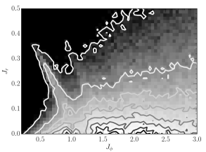
Figure 1: The phase-space distribution of the particles in simulation 50M of Sellwood (2012) at time 1400, presented as a function of angular momentum, denoted by $J_{\phi}$, and the radial action, denoted by $J_{r}$. Circular orbits are characterized by $J_{r}=0$. The contours of constant stellar phase-space density are evenly spaced between 2.5 % and 95 % of the maximum value of the DF (estimated as the mean of the 10 highest-valued pixels). Three grooves can be identified where circular orbits are depopulated around the angular momentum values $J_{\phi}\approx 1.2$, $1.55$, and $1.90$.

While this half-mass Mestel disc is linearly stable, this does not mean that it cannot evolve secularly through finite-$N$ effects. In order to maximally elucidate the underlying dynamics, Sellwood (2012) and Fouvry et al. (2015) consider only gravitational forces up to the $m=2$ harmonic in their studies of the evolution of this disc model. Therefore, we will likewise only consider $m=2$ spiral patterns in the remainder.

As shown by Sellwood (2012) and Fouvry et al. (2015), swing-amplified finite-$N$ stellar density fluctuations in this Mestel disc transport angular momentum away from their inner Lindblad resonances (ILR) and scatter stars away from (near-)circular orbits around certain angular momenta. If a spiral wave is time-independent in a co-rotating coordinate frame then each star evolves along a track of constant Jacobi integral, $E_{\mathrm{J}}$, given by

$$E_{\mathrm{J}}=E+\Omega_{\mathrm{p}}J_{\phi},$$ (7)

with $\Omega_{\mathrm{p}}$ the wave’s pattern speed. The interaction between the stars and transient swing-amplified patterns induces stellar migration through action space, changing the stars’ binding energy and angular momentum but preserving their Jacobi integral. At a pattern’s ILR, this pushes stars away from circular orbits towards orbits with lower angular momentum $J_{\phi}$ and higher values of the radial action $J_{r}$. Hence, the DF develops what we here refer to as grooves (loci around constant $E_{\mathrm{J}}$-values where stars have diffused away from high-$J_{\phi}$ orbits, leaving behind a depleted DF) and ridges (loci around constant $E_{\mathrm{J}}$-values where stars have diffused towards high-$J_{r}$ orbits, causing an enhanced DF).

In Figure 1, we show the DF of the half-mass Mestel disc, grooved on the long term by the non-linear evolution of swing-amplified particle-shot noise, as obtained in simulation 50M of Sellwood (2012) (see also Figure 7 in Sellwood (2012) and Figure 4 in Fouvry et al. (2015)). Three grooves can be identified where circular orbits are depopulated around angular momentum values $J_{\phi}\approx 1.2$, $1.55$, and $1.90$.

Concurrent with the appearance of these grooves in action space, the stellar disc develops a set of vigorously growing spiral patterns whose amplitudes exponentiate with time (see Figure 2 in Sellwood (2012)). The most vigorous among these modes has a rotation frequency $\omega=m\Omega_{\mathrm{p}}\approx 0.55$ (see Figure 4 in Sellwood (2012)). It cannot be an eigenmode of the ungrooved half-mass Mestel disc because it is known to be linearly stable. Since the mode already appears in the linear regime it is unlikely to be caused by non-linear mode coupling (Masset & Tagger, 1997). Randomizing the azimuthal particle positions does not prevent the pattern’s growth, quite on the contrary, so any non-axisymmetric features that grew during the disc’s first phase of evolution cannot have caused this growing mode (see Figure 5 in Sellwood (2012)). The fact that it grows exponentially with time suggests that it is a true eigenmode particular to the grooved half-mass Mestel disc.

Using linear stability analysis, we now show that the vigorously exponentiating patterns observed by Sellwood (2012) are indeed eigenmodes of the grooved half-mass Mestel disc. For this, we use pyStab, a Python/C++ computer code to analyse the stability of a responsive, self-gravitating razor-thin stellar disc embedded in the gravitational field of a rigid axisymmetric or spherically symmetric central bulge and dark-matter halo. The details of the mathematical formalism behind this code and of its implementation can be found in Vauterin & Dejonghe (1996), Dury et al. (2008), and De Rijcke & Voulis (2016) so we will not repeat these here in detail. We provide a brief overview of the formalism and of the employed values of some numerical parameters of the code in Appendix A.

3 Mode-analysis of the grooved half-mass Mestel disc

3.1 The fiducial grooved half-mass Mestel disc

We first mimicked the grooves visible in the DF of simulation 50M (see Fig. 1) of Sellwood (2012) by multiplying the DF $F_{0}(E,J_{\phi})$ with “groove functions” of the form

$$f_{\rm groove}(x)=1+\frac{a}{(1-x)^{\alpha}}+b+cx+dx^{2},$$ (8)

with $x$ varying along a line of constant Jacobi integral, normalized such that $x=0$ at the circular orbit and $x=1$ at the radial orbit. Each groove function differs from 1 only inside a narrow region of width $2w$ centered on a given Jacobi integral. If $f_{\rm groove}(x)>1$, the phase-space density is increased; if $f_{\rm groove}(x)<1$, the phase-space density is decreased.

Based on Figure 1, we identify three angular momenta where circular orbits are significantly depopulated: at $J_{\phi}\approx 1.2$ (first groove), $1.55$ (second groove), and $1.9$ (third groove), corresponding to the ILR of waves with pattern speeds $\Omega_{\mathrm{p}}=0.244$, $0.189$, and $0.154$, respectively. We will henceforth refer to the half-mass Mestel disc with these three grooves as the fiducial grooved half-mass Mestel disc.

Table 1: The parameter values employed in the “groove function” $f_{\rm groove}$ that defines the profile of each groove (cf. equation 8).

	$\alpha$	$w$	$a$	$b$	$c$	$d$
first groove	11	0.29	0.474	-0.044	-5.219	-44.796
second groove	6	0.10	0.562	0.388	-3.371	-15.619
third groove	6	0.12	0.081	0.869	-0.486	-3.242

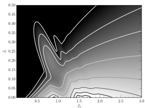
Figure 2: The DF of the fiducial grooved half-mass Mestel disc. The contours of constant stellar phase-space density are evenly spaced between 2.5 % and 95 % of the maximum value of the DF.

At the first groove, at $J_{\phi}\approx 1.2$, the value of the DF decreases by 57 % while, at the second and third groove, at $J_{\phi}\approx 1.55$ and $1.9$, the value of the DF decreases by 5 %. The first groove leads to a marked population increase of the lower angular momentum/higher radial action orbits, which is mimicked here by setting $\alpha=11$ in equation (8). The second and, especially, the third groove show much less pronounced DF increases towards low angular momentum orbits so we choose $\alpha=6$ for these. For each groove, the parameters $w$, $a$, $b$, $c$, and $d$ are chosen such that the grooves visible in Figure 1 are adequately reproduced, cf. Figure 2 and Table 1. We took care to conserve the total mass of the stellar disc to within a few tenths of a percent.

Table 2: The eigenmodes of the half-mass Mestel disc with three grooves at $J_{\phi}=1.2$, $1.55$, and $1.9$. The complex mode frequency is denoted by $\omega$. The radii of the main resonances (ILR, CR, OLR) are indicated and resonances that (approximately) overlap with the position of a groove are printed in boldface. The physical nature of each mode (global or groove mode) is given in the last column.

$\omega$	ILR	CR	OLR	type
$0.597+0.013{{\mathrm{i}}}$	0.98	3.35	5.72	global mode
$1.662+0.004{{\mathrm{i}}}$	0.35	1.20	2.01	groove mode
$0.465+0.001{{\mathrm{i}}}$	1.26	4.30	7.34	global mode
$1.101+0.000{{\mathrm{i}}}$	0.53	1.82	3.10	groove mode

3.2 Linear stability analysis of the fiducial grooved Mestel disc

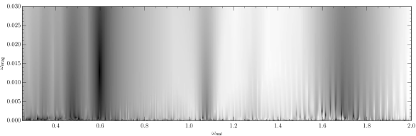
Figure 3: The quantity $\min\left|\lambda(\omega)-1\right|$ in the complex frequency plane of the fiducial grooved half-mass Mestel disc. An eigenmode lives wherever this quantity is zero (dark regions).

As explained in Appendix A, each eigenmode corresponds to a complex frequency $\omega$ for which the matrix ${\mathcal{C}}(\omega)$, defined in equation (28), has a unity eigenvalue. In Figure 3, we plot the quantity $\min\left|\lambda(\omega)-1\right|$ in the complex frequency plane of the fiducial grooved half-mass Mestel disc. This quantity is zero at the loci of the eigenmodes.

The complex frequencies $\omega$ of the dominant eigenmodes retrieved with pyStab for the fiducial grooved half-mass Mestel disc are listed in Table 2, along with the radii where the main resonances (ILR, CR, OLR) occur, with CR the corotation resonance radius and OLR the Outer Lindblad Resonance radius. Resonances that (approximately) overlap with the position of a groove are printed in boldface. For the Mestel disc, the resonance radii $r_{\mathrm{res},\ell}$ of an $m$-armed mode with pattern speed $m\Omega_{\mathrm{p}}=\omega_{\mathrm{real}}$, with $\omega_{\mathrm{real}}$ the real part of the mode frequency, are given by

$$r_{\mathrm{res},\ell}=\left(m+\sqrt{2}\ell\right)\frac{1}{\omega_{\mathrm{real}}}.$$ (9)

Here, $\ell=0$ gives the CR while $\ell=\pm 1$ give the Lindblad resonances.

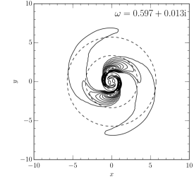
Figure 4: Top panel: the positive part of the surface density perturbation of the $m=2$ global mode with frequency $0.597+0.013{{\mathrm{i}}}$ of the fiducial grooved half-mass Mestel disc. The contour values increase linearly between 1 % and 99 % of the maximum surface density value. The full line indicates the position of the first, main groove and dashed lines mark the mode’s ILR, CR, and OLR. Bottom panel: the surface density perturbation of mode 50Mc from the $N$-body simulations by Sellwood (2012). Dotted lines mark the Lindblad resonances while the full line marks the CR radius.

3.3 The $\omega=0.597+0.013{{\mathrm{i}}}$ mode: a cavity mode

The most rapidly growing global spiral mode has a pattern speed $m\Omega_{\mathrm{p}}=0.597$ which places its ILR at a radius of 0.98, very near the inner edge of the first groove, while its OLR occurs at a radius of 5.72. The other global spiral mode, with a pattern speed $m\Omega_{\mathrm{p}}=0.465$, has a negligible growth rate (this is actually the fastest growing member of a cluster of eigenmodes with pattern speeds between 0.45 and 0.5, cf. Figure 3). The surface density of the dominant global spiral mode is plotted in Figure 4 (top panel) where we compare it with the dominant spiral pattern found in the $N$-body simulations reported in Sellwood (2012) (bottom panel). The frequency of the emerging pattern is estimated at $\omega\approx 0.577+0.018{{\mathrm{i}}}$ in simulation 50M and at $\omega\approx 0.599+0.016{{\mathrm{i}}}$ in simulation 50Mc. We find $\omega=0.597+0.013{{\mathrm{i}}}$ for the dominant eigenmode of the fiducial grooved Mestel disc. This good agreement between the pattern speeds leads us to confirm that we are, in fact, seeing the same mode in the linear stability analysis and in the $N$-body simulations.

3.3.1 Mode generating mechanism: linear stability analysis

As noted by Sellwood & Carlberg (2014), a phase-space groove induces a spatially localized change of the velocity with which spiral waves can be radially propagated through the disc. A groove locally changes the “impedance” of the stellar disc. Using the suggestive analogy of waves being partially reflected at the junction between two strings with different mass densities (and hence different wave velocities), these authors argue that stellar density waves impacting radially inward on a phase-space groove will, likewise, be partially reflected outward again. This creates the possibility of setting up a resonant cavity within which inwards moving waves are (partially) reflected back out again by the groove and outwards moving waves are reflected back inwards at corotation, thus creating a standing wave pattern.

In the WASER feedback cycle (Toomre, 1969; Mark, 1976), an ingoing short-wavelength trailing wave is reflected from the unresponsive, dynamically hot disc interior (if the Toomre $Q$ parameter (Toomre, 1964) rises sufficiently rapidly towards small radii) into an outgoing long-wavelength trailing wave. At CR, this wave overreflects into an ingoing and an outgoing short-wavelength traling wave. Hence, the WASER only involves trailing waves. Moreover, it leads to rather modest wave amplifications and then only for low $Q$ values. Much more impressive amplifications can be obtained by the swing amplifier feedback cycle (Toomre, 1977, 1981; Bertin et al., 1989). In this theory, an ingoing trailing wave is reflected from the galaxy center as an outgoing leading wave. Around CR, this wave is overreflected into an outgoing and an ingoing trailing wave at which point amplification factors of $1-2$ orders of magnitude can be achieved. Significant amplification occurs for discs with $Q\apprle 2$. Interference between the leading and trailing waves within the resonant cavity is expected to produce a growing eigenmode with a “lumpy” density distribution (Athanassoula, 1984; Binney & Tremaine, 2008).

If the inner $Q$-profile of the half-mass Mestel disc were steep enough to reflect ingoing waves outwards again, it would already have done so in the ungrooved model and that model is linearly stable. Therefore, it is unlikely that the WASER feedback cycle is responsible for the growth of the global modes in the grooved half-mass Mestel disc. On the other hand, the Toomre $Q$ parameter is smaller than $2.0$ in a large part of disc, between radii in the range $\approx 1.4-9.0$, and hovers around a value of $1.5$ between radii in the range $\approx 2.0-6.0$. From the famous “dust to ashes” figure of Toomre (1981), it is clear that swing amplification in the $Q=1.5$, $X=k_{\rm crit}r/m=2$ half-mass Mestel disc without inner or outer cut-outs can boost wave amplitudes by a factor $\sim 30$ (which significantly hastens the disc’s secular dynamics). Unfortunately, those amplified waves are subsequently absorbed at the ILR. This is, however, not an issue for the grooved half-mass Mestel disc. In the case of waves with a pattern speed $m\Omega_{\mathrm{p}}=0.597$, corresponding to the dominant global mode of the fiducial grooved half-mass Mestel disc, the ILR (at a radius of 0.98) is shielded by the reflective first groove (around a radius of 1.2). Moreover, this dominant global mode clearly has a “lumpy” density distribution (cf. Figure 4), indicative of interference between leading and trailing waves.

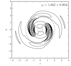
Figure 5: The positive part of the surface density perturbation of the $m=2$ mode of the fiducial grooved half-mass Mestel disc, with frequency $\omega=1.662+0.004{{\mathrm{i}}}$. The contour values increase linearly between 1 % and 99 % of the maximum surface density value. The dashed lines mark the modes’ ILR, CR, and OLR and the full line indicates the position of the first, main groove.

3.3.2 Mode generating mechanism: WKB arguments

If an eigenmode is indeed a standing wave built from wave packets traveling inside a resonance cavity between radii $r_{\mathrm{inf}}$ and $r_{\mathrm{sup}}$ then it must obey the quantum condition

$$\oint_{r_{\mathrm{inf}}}^{r_{\mathrm{sup}}}k\left(\omega_{\mathrm{real}},r\right)\mathrm{d}r=\pi$$ (10)

where $k$ is the radial wavenumber of the waves. The mode’s growth rate $\omega_{\mathrm{im}}=\Im\{\omega\}$ then follows from the relation

$$\frac{1}{\omega_{\mathrm{im}}}\oint_{r_{\mathrm{inf}}}^{r_{\mathrm{sup}}}\frac{\mathrm{d}r}{v_{\mathrm{g}}(r)}=\frac{\ln 2}{2},$$ (11)

with $v_{\mathrm{g}}(r)$ the radial group velocity of the traveling wave patterns (Mark, 1977; Bertin, 2014). Hence, the narrower the cavity and the larger the group velocity, the stronger the growth. These integrals are to be performed over a full circle between their lower and upper bounds.

In the WKBJ limit, the dispersion relation for traveling waves is given by

$$\kappa^{2}\left(1-s^{2}\right)=2\pi G\Sigma\left|k\right|{\mathcal{F}}(s,\chi)\mathrm{e}^{-\varepsilon\left|k\right|}.$$ (12)

Here,

$$s=\frac{\omega_{\mathrm{real}}-m\Omega}{\kappa}\,\,\mathrm{and}\,\,\chi=\left(\frac{k\sigma_{r}}{\kappa}\right)^{2},$$ (13)

with $\Omega$ and $\kappa$ the angular and epicycle frequency of near-circular orbits, respectively (Kalnajs, 1965; Lin & Shu, 1966). The reduction factor on the right-hand side of this equation is the product of two factors: an exponential factor caused by the Plummer softening with softening length $\varepsilon$ (Romeo, 1994), for which we adopt the value $\varepsilon=1/8$, and the well-known reduction factor

$${\mathcal{F}}(s,\chi)=2\left(1-s^{2}\right)\frac{\mathrm{e}^{-\chi}}{\chi}\sum_{n\geq 1}\frac{I_{n}(\chi)}{1-\frac{s^{2}}{n^{2}}},$$ (14)

with $I_{n}$ a modified Bessel function of the first kind, due to the stellar velocity velocity dispersion. This latter expression is only correct for a Schwarzschild DF so the following results must be regarded as approximate. The group velocity $v_{\mathrm{g}}$ of a wave packet centered on wave number $k$ is given by

$$v_{\mathrm{g}}=\frac{\partial\omega_{\mathrm{real}}}{\partial k}.$$ (15)

From the dispersion relation stated above, we can derive the relation

$$\left[\frac{2s}{1-s^{2}}+\mathrm{e}^{\varepsilon\left|k\right|}\frac{\partial\ln\mathcal{F}}{\partial s}\right]v_{\mathrm{g}}=$$

$$-\frac{\kappa}{k}\left[1-\varepsilon\left|k\right|+2\mathrm{e}^{\varepsilon\left|k\right|}\frac{\partial\ln\mathcal{F}}{\partial\ln\chi}\right]$$ (16)

for the group velocity. The partial derivatives of the reduction factor $\mathcal{F}$ that figure in this equation can be evaluated analytically as

$$\frac{\partial\mathcal{F}}{\partial\chi} =\left(1-s^{2}\right)\frac{\mathrm{e}^{-\chi}}{\chi}\sum_{n\geq 1}\frac{I_{n-1}-2\left[1+\frac{1}{\chi}\right]I_{n}+I_{n+1}}{1-\frac{s^{2}}{n^{2}}},$$

$$\frac{\partial\mathcal{F}}{\partial s} =-4s\frac{\mathrm{e}^{-\chi}}{\chi}\sum_{n\geq 2}\frac{1-\frac{1}{n^{2}}}{1-\frac{s^{2}}{n^{2}}}I_{n},$$ (17)

where all Bessel functions have $\chi$ as argument. We terminate the infinite sums in the evaluation of this reduction factor and its derivatives when a relative accuracy of $10^{-6}$ has been obtained.

We now wish to compute the frequency of a growing standing wave in the half-mass Mestel disc with a groove at a radius $r_{\mathrm{groove}}$, which is supposed to reflect incoming wave packets back out again, using this analytical theory. For a given real frequency $\omega_{\mathrm{real}}$, we first compute the inner radius of the forbidden region around CR, where the dispersion relation (12) admits no real solutions for $k$. This we equate to the outer radius of the resonance cavity, $r_{\mathrm{sup}}$. For the inner radius, $r_{\mathrm{inf}}$, we use the maximum of the groove radius and the wave’s ILR radius. In practice, this always turned out to be the groove radius.

For any radius $r$ inside the resonance cavity, we then find the two positive solutions $k_{\mathrm{short}}(\omega_{\mathrm{real}},r)$ and $k_{\mathrm{long}}(\omega_{\mathrm{real}},r)$ of the dispersion relation (12). The quantum condition (10) can be rewritten as

$$\oint_{r_{\mathrm{inf}}}^{r_{\mathrm{sup}}}k\left(\omega_{\mathrm{real}},r\right)\mathrm{d}r$$

$$=\int_{r_{\mathrm{inf}}}^{r_{\mathrm{sup}}}\left[k_{\mathrm{short}}(\omega_{\mathrm{real}},r)+k_{\mathrm{long}}(\omega_{\mathrm{real}},r)\right]\mathrm{d}r=\pi.$$ (18)

Numerical root finding finally allows us to solve this equation for the real frequency $\omega_{\mathrm{real}}$ in case the disc supports a cavity mode. Equation (16) yields the group velocities, $v_{\mathrm{g},{\mathrm{short}}}(r)$ and $v_{\mathrm{g},{\mathrm{long}}}(r)$, of the short and long branch waves, respectively. These are then inserted into equation (11), which can be rewritten as

$$\oint_{r_{\mathrm{inf}}}^{r_{\mathrm{sup}}}\frac{\mathrm{d}r}{v_{\mathrm{g}}(r)} =\int_{r_{\mathrm{inf}}}^{r_{\mathrm{sup}}}\left[\frac{1}{v_{\mathrm{g},{\mathrm{short}}}(r)}+\frac{1}{v_{\mathrm{g},{\mathrm{long}}}(r)}\right]\mathrm{d}r$$

$$=\frac{\ln 2}{2}\omega_{\mathrm{im}}.$$ (19)

This, finally, provides us with an estimate for the growth rate $\omega_{\mathrm{im}}$ of the growing mode.

For the fiducial value of the groove radius, $r_{\mathrm{groove}}=1.2$, this yields the analytical frequency estimate $\omega=0.510+0.017\mathrm{i}$. This is tantalizingly close to the value $\omega=0.597+0.013\mathrm{i}$ that we derived from the full linear theory. Together with all the arguments given above, this can be taken as evidence for the idea that the dominant global mode of the grooved Mestel disc is caused by swing-amplified traveling wave packets inside a resonance cavity between the groove – rendered reflective by the depopulation of near-circular orbits – and the mode’s CR.

3.4 The $\omega=1.662+0.004{{\mathrm{i}}}$ mode: a groove mode

Glancing back at Table 2, the second most unstable mode of the grooved Mestel disc, depicted in Figure 5, has properties that suggest that it is a groove mode caused by the first groove, depopulating circular orbits around angular momentum $J_{\phi}=1.2$. There actually appears to exist a cluster of eigenmodes with pattern speeds very close to this value, cf. Figure 3, of which this is the most rapidly growing member.

Sellwood & Kahn (1991) describe growing instabilities with their CR at a sharp groove, i.e. a local depression in the stellar density distribution, that are an instance of the negative-mass instability (Lovelace & Hohlfeld, 1978). These authors show that such groove modes originate from the coupling of two waves, one on each side of the groove, with their corotation resonance inside the groove. The wavy displacements of disc material at the groove’s edges couple across the groove through gravity. Thus, local overdensities can exchange angular momentum in such a way that material on the groove’s inner edge gains angular momentum and is pulled outwards while material on the groove’s outer edge loses angular momentum and is pulled inwards. This counteracts the disc’s shear and facilitates mass clumping. Thus, the amplitude of these mass displacements grows exponentially with time. The rest of the pattern can then be explained as the disc’s response to these growing overdensities via the mechanism described by Julian & Toomre (1966).

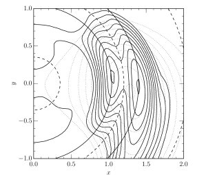
Figure 6: Close-up view of the density peak of the $\omega=1.662+0.004{{\mathrm{i}}}$ groove mode from Fig. 5. Full-line contours trace the surface density perturbation (in 10 equidistant steps between 1 % and 99 % of its maximum value) while the dotted contours trace the mode’s gravitational binding potential (in 10 equidistant steps between 1 % and 99 % of its maximum value). Dashed circles mark the loci of the mode’s ILR, CR, and OLR. The two full-line circles demarcate the region where the DF has been reduced by more than 50 %, which could be taken as a measure for the width of the groove.

The CR of the $\omega=1.662+0.004{{\mathrm{i}}}$ mode indeed sits squarely inside the first groove, cf. Figure 6. It is also clear from this figure that the mode, as expected for a groove mode, consists of two density peaks sitting on either side of the groove with a gravitational potential peak between them. This suggests this is a groove mode caused by the first groove. There also appears to exist a neutral eigenmode with pattern speed $m\Omega_{\mathrm{p}}=1.101$ which can, likewise, be interpreted as a groove mode caused by the third groove. Its vanishing growth rate explains why it did not appear in the simulations reported by Sellwood (2012).

4 Discussion

4.1 The number of grooves

The presence of the minor second and third groove has little bearing on the existence of the modes although it does slightly impact their frequencies. For instance, if we remove these two minor grooves, keeping only the deep and wide first groove, the main global mode is retrieved with a frequency $\omega=0.603+0.016{{\mathrm{i}}}$, with its ILR sitting at a radius of 0.97, still just inside the inner edge of the groove. The groove mode now has a frequency $\omega=1.695+0.003{{\mathrm{i}}}$. Its CR, now at a radius 1.18, again falls inside the groove. The remaining groove is obviously instrumental to the existence of these modes. Without it, the grooveless half-mass Mestel disc is, as already mentioned, linearly stable.

4.2 The groove profile

A groove consists both of a depletion of circular orbits and an overpopulation of more radial orbits. In order to test which of these two features is actually causing the modes in the grooved Mestel disc, we first computed the eigenmode spectrum of a model with the fiducial groove function modified according to the prescription

$$f_{\rm groove}(x)\rightarrow\max\left\{1,f_{\rm groove}(x)\right\}$$ (20)

so that no stars are ever removed but only added. This removes the grooves at the loci of near-circular orbits but leaves the ridges at more radial orbits in place. This particular model turned out to have a single (barely) growing global eigenmode at $\omega=0.611+0.001{{\mathrm{i}}}$. The high-frequency mode of the fiducial model is completely absent.

Next, we computed the eigenmode spectrum of a model with the fiducial groove function modified according to the prescription

$$f_{\rm groove}(x)\rightarrow\min\left\{1,f_{\rm groove}(x)\right\}$$ (21)

so that no stars are ever added but only removed. This removes the ridges at more radial orbits but leaves the grooves at the loci of near-circular orbits in place. This model has two growing eigenmodes, at $\omega=0.593+0.013{{\mathrm{i}}}$ and $\omega=1.663+0.003{{\mathrm{i}}}$. These are virtually the same as the eigenmodes of the fiducial grooved Mestel disc. Likewise, we analysed a model in which the depth of the three grooves of the fiducial model is kept constant along lines of constant Jacobi integral. In other words: the first groove depresses the DF by 57 % and the second and third groove by 5 % everywhere along the groove in question. The stellar mass of this model is a bit smaller than in the fiducial model but this has no apparent consequences. Indeed, this model’s mode spectrum is almost identical to that of the fiducial model.

Putting these results together, we are led to the conclusion that it is the depopulation of the near-circular orbits and not the overpopulation of the radial orbits that is crucial to the existence of the growing eigenmodes of the grooved Mestel disc. This corroborates the results from Sellwood & Kahn (1991), who use an approximate analytical computation to demonstrate that grooves are destabilizing while ridges are not.

4.3 The groove depth

Table 3: Reprise of Table 2, with the eigenmodes of the half-mass Mestel disc with three grooves at $J_{\phi}=1.2$, $1.55$, and $1.9$ with various depths. The depth of the first groove, expressed relative to its fiducial depth, is indicated in the first column. The depths of the other two grooves are varied proportionally. The complex mode frequency is denoted by $\omega$. The radii of the main resonances (ILR, CR, OLR) are indicated and resonances that (approximately) overlap with the position of a groove are printed in boldface. The physical nature of each mode (global or groove mode) is given in the last column.

depth	$\omega$	ILR	CR	OLR
155 %	$0.582+0.019{{\mathrm{i}}}$	1.00	3.44	5.86	global mode
	$1.709+0.016{{\mathrm{i}}}$	0.34	1.17	2.00	groove mode
	$1.078+0.010{{\mathrm{i}}}$	0.54	1.86	3.17	groove mode
	$0.471+0.001{{\mathrm{i}}}$	1.24	4.25	7.25	global mode
100 %	$0.597+0.013{{\mathrm{i}}}$	0.98	3.35	5.72	global mode
	$1.662+0.004{{\mathrm{i}}}$	0.35	1.18	2.01	groove mode
	$0.465+0.001{{\mathrm{i}}}$	1.26	4.31	7.35	global mode
80 %	$0.604+0.008{{\mathrm{i}}}$	0.97	3.31	5.65	global mode
60 %	$0.611+0.002{{\mathrm{i}}}$	0.96	3.27	5.59	global mode

We varied the depths of the grooves, keeping their respective depths in proportion. This leads to the eigenmode spectra listed in Table 3. Clearly, the deeper the grooves, the more rapidly the mode with pattern speed $m\Omega_{\mathrm{p}}\approx 0.6$ grows. This confirms the finding by Sellwood (2012); Sellwood & Carlberg (2014) that new instabilities only start to grow when the phase-space grooves are sufficiently deep.

Moreover, new eigenmodes appear as the grooves are deepened. For instance, the mode with frequency $\omega=1.078+0.010{{\mathrm{i}}}$, which appears in the spectrum of the model with a first groove that is 1.55 times as deep as in the fiducial model, is a groove mode with its CR at the position of the third groove, at angular momentum $J_{\phi}=1.9$. This corroborates the results from Sellwood & Kahn (1991), who find that a groove of a given width needs to exceed a critical depth before it can create a groove mode. Using approximate analytical calculations, these authors predict the critical depth to be proportional to the groove’s width, which is in rough agreement with the required groove depths we observe here.

4.4 The position of the grooves

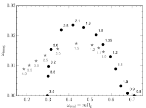
Figure 7: Position of the dominant $m=2$ eigenmode in the complex frequency plane of the half-mass Mestel disc as a function of groove position, computed using the full linear theory (black bullets) and using the approximate calculation from paragraph 3.3.2 (grey stars). The angular momentum of the first groove takes on values between $J_{\phi}=0.8$ and $J_{\phi}=3.5$, as indicated next to each data point. The ratio of the angular momentum of the second and the third groove to that of the first groove is kept constant, causing the grooves to jointly sweep through phase space. The fiducial grooved Mestel disc corresponds to $J_{\phi}=1.2$.

An investigation of the role of the positions of the grooves is not possible with the techniques of Sellwood (2012) and Fouvry et al. (2015), where the grooves grow due to stellar dynamics and their position is determined by the physics of the problem. Here, on the contrary, we have full control over the positions of the grooves. We simply change the angular momentum of the circular orbits depleted by the first groove between 0.8 and 3.5 while maintaining a constant pattern speed ratio between the three grooves and keeping all other groove properties constant. This causes the grooves to jointly sweep accross the phase-space region with the highest stellar density.

The result is plotted in Figure 7. Here, the black bullets indicate the frequency of the dominant global eigenmode in the complex frequency plane for different positions of the grooves. Each data point is labeled with the angular momentum $J_{\phi}$ of the circular orbits depleted by the first groove as it sweeps through phase space. Growing eigenmodes are triggered only if the grooves fall in a “responsive” region of phase space (see also De Rijcke & Voulis (2016)). In this case, this means a groove carving into the most densely populated region of phase space: that of the circular orbits with radii between 1.5 and 2.5. A groove falling outside this region has a much less marked effect, as can be expected from removing stars from sparsely populated phase-space surroundings.

The grey stars in Figure 7 show the analytical estimate for the frequency of the dominant global eigenmode as a function of groove position, using the analytical formalism detailed in paragraph 3.3.2. Each star is labeled with the angular momentum $J_{\phi}$ of the circular orbits depleted by the first groove. This estimate, derived from an analytical calculation based on the assumption that we are dealing with a cavity mode between the groove radius and the forbidden region around corotation, is clearly in rough agreement with the full linear theory result. Given the approximations underlying this calculation, this level of agreement is actually surprisingly good and can be taken as strong evidence for our interpretation of the dominant global eigenmode as a cavity mode.

4.5 Gravitational softening

Table 4: The eigenmodes of the unsoftened half-mass Mestel disc with three grooves at $J_{\phi}=1.2$, $1.55$, and $1.9$. The complex mode frequency is denoted by $\omega$. The radii of the main resonances (ILR, CR, OLR) are indicated and resonances that (approximately) overlap with the position of a groove are printed in boldface. The physical nature of each mode (global or groove mode) is given in the last column.

$\omega$	ILR	CR	OLR	type
$1.7260+0.068{{\mathrm{i}}}$	0.34	1.16	1.98	groove mode
$0.6740+0.040{{\mathrm{i}}}$	0.87	2.97	5.06	global mode
$0.5470+0.011{{\mathrm{i}}}$	1.07	3.65	6.24	global mode
$1.0650+0.004{{\mathrm{i}}}$	0.55	1.88	3.21	groove mode
$0.5420+0.003{{\mathrm{i}}}$	1.08	3.69	6.29	global mode
$0.4200+0.001{{\mathrm{i}}}$	1.39	4.76	8.13	global mode

Gravitational softening with a Plummer kernel with softening length $\varepsilon=1/8$, as employed by Sellwood (2012), has a very strong impact on the eigenmode spectrum of the grooved Mestel disc. In Table 4, we list the dominant eigenmodes of the unsoftened grooved Mestel disc model. Without gravitational softening, the groove modes grow much faster than in the softened model. For instance, the groove mode caused by the first groove is now by far the fastest growing mode. The global modes around $m\Omega_{\mathrm{p}}\approx 0.45$ and $m\Omega_{\mathrm{p}}\approx 0.6$ appear to be relatively unaffected by softening but they are now surpassed in growth rate by the groove modes. Moreover, new eigenmodes appear in the spectrum of the unsoftened model: the very rapidly growing mode at $\omega=0.6740+0.040{{\mathrm{i}}}$ and the slowly growing mode at $\omega=0.5420+0.003{{\mathrm{i}}}$.

5 Conclusions

We have studied the linear stability of a half-mass Mestel disc, with a distribution function modified with phase-space grooves like the ones found in the works of Sellwood (2012), Fouvry et al. (2015), and Fouvry (2017). The ungrooved model is linearly stable so that any modes found in the grooved models must somehow be related to the presence of the grooves. Since we compare our linear stability computations with $N$-body simulations, we take into account the effects of gravitational softening (De Rijcke et al., 2018).

In the fiducial grooved model, we mimic the grooves visible in the DF of the $N$-body simulation 50M of Sellwood (2012) and show that this model has $m=2$ eigenmodes with properties very close to the two-armed spiral patterns visible in its simulated analog. We argue that, at least in this case, the dominant new eigenmode is a cavity mode, living inside a resonance cavity between the groove – rendered reflective by the removal of stars from near-circular orbits – and the forbidden region around corotation (Mark, 1977; Bertin, 2014). Other, more slowly growing new eigenmodes can be interpreted as groove modes (Sellwood & Kahn, 1991).

This confirms the suggestion put forward in Sellwood (2012) and Sellwood & Carlberg (2014) that grooves can be a potent source of new, rapidly growing eigenmodes. These grooves are produced by a series of uncorrelated swing-amplified waves, sourced by the collisional, finite-$N$ nature of any self-gravitating stellar system. In other words: it is possible for an isolated, linearly stable stellar disc, initially without recourse to any growing eigenmodes that can transport its angular momentum outwards as desired by the second law of thermodynamics (Lynden-Bell & Kalnajs, 1972; Zhang, 1996), to spontaneously become linearly unstable via the formation of grooves in phase space through finite-$N$ dynamics. The simple model of the half-mass Mestel disc with inner and outer cut-outs serves as a template for more realistic galaxy models, equipped with more plausible bulge and halo components. The idea is that the dynamical processes leading to the vigorously growing spiral modes in this Mestel disc also explain the spirals in $N$-body simulations of more complex galaxy models, something which needs to investigated further.

Ultimately, one hopes that understanding these dynamical processes in simulated galaxies furthers our understanding of the growth and maintenance of spiral structure in real galaxies. Real spiral galaxies evidently contain much more stars than the $\sim 10^{6}-10^{8}$ particles that are routinely used in $N$-body simulations and their stellar bodies are, therefore, much smoother than those of their simulated counterparts. As shown by Sellwood (2012) and Fouvry et al. (2015), the time at which the disc’s collisional dynamics has carved sufficiently deep phase-space grooves and the new eigenmodes start to manifest themselves grows with the number $N$ of particles so one can wonder whether the mechanism discussed here actually applies to real galaxies. However, whereas the stellar bodies of real galaxies are perhaps much smoother than those of simulated galaxies, they possess other potent sources of gravitational “noise”, such as giant molecular clouds or globular clusters moving in or through the stellar disc (D’Onghia et al., 2013), orbiting satellite dwarf galaxies (Martínez-Delgado et al., 2008; Laporte et al., 2018), and dark-matter sub-halos (Dubinski et al., 2008; Chequers et al., 2018; Hu & Sijacki, 2018), that could play the same role as the particle noise present in simulations. Moreover, stellar discs are dynamically cold systems so that through self-gravity any perturbation is dressed by a polarisation cloud, which further hastens the disc’s evolution.

Appendix A Gravitationally softened linear stability analysis

In short: an axially symmetric disc galaxy model is characterized by a distribution function $F_{0}(E,J_{\phi})$, with $E$ the specific binding energy and $J_{\phi}$ the specific angular momentum of a stellar orbit, and a (positive) gravitational binding potential $V_{0}(r)$. pyStab retrieves those complex frequencies $\omega$ for which a spiral-shaped perturbation of the form

$$V_{\rm pert}(r,\phi,t)=V_{\rm pert}(r)\mathrm{e}^{\mathrm{i}(m\phi-\omega t)}$$ (22)

constitutes an eigenmode with infinitesimal amplitude. Here, $(r,\phi)$ are polar coordinates in the stellar disc, $V_{\rm pert}(r)$ is a complex function quantifying the mode’s amplitude and phase, $m$ is its multiplicity, $\Omega_{\mathrm{p}}=\Re\{\omega\}/m$ its pattern speed, and $\Im\{\omega\}$ its growth rate. A general perturbing potential can always be expanded in such spirals and, for infinitesimal amplitudes, these can be studied independently from each other.

In essence, pyStab solves the first-order collisionless Boltzmann equation to find the response distribution function $f_{\rm resp}(r,\phi,v_{r},v_{\phi},t)$ produced by a given perturbation $V_{\rm pert}(r,\phi,t)$. This response distribution function generates a response density given by

$$\Sigma_{\rm resp}(r,\phi,t)=\int f_{\rm resp}(r,\phi,v_{r},v_{\phi},t)\mathrm{d}v_{r}\mathrm{d}v_{\phi},$$ (23)

which, in turn, corresponds to a response gravitational potential given by

$$V_{\rm resp}(\vec{r})=G\int\Sigma_{\rm resp}(\vec{r}^{\prime})\,\psi(|\vec{r}-\vec{r}^{\prime}|)\,\mathrm{d}^{2}\!\vec{r}^{\prime},$$ (24)

with $\psi$ the inter-particle interaction potential. For Newtonian gravity, one evidently has

$$\psi(|\vec{r}-\vec{r}^{\prime}|)=\frac{1}{|\vec{r}-\vec{r}^{\prime}|},$$ (25)

while Plummer softened interactions are quantified by the choice

$$\psi(|\vec{r}-\vec{r}^{\prime}|)=\frac{1}{\sqrt{\varepsilon^{2}+|\vec{r}-\vec{r}^{\prime}|^{2}}},$$ (26)

with $\varepsilon$ the softening length.

Since we want to validate our approach by comparing particular results with the numerical simulations presented in Sellwood (2012), we mimic the strategies employed in that work, in particular the softening method. There, the initial condition is generated by sampling stellar particles from the distribution function $F_{0}(E,J)$ evaluated using the mean Newtonian gravitational potential $V_{0}(r)$, independent of the gravitational softening that is employed to evolve the particles through time. Moreover, the axially symmetric force field of the base state is evaluated correctly, i.e. without softening, while the non-axisymmetric force field of the growing waves is softened. Therefore, in our search for unstable models, we only implement Plummer-type softening in the response potential $V_{\rm resp}(r,\theta,t)$, but not in the axially symmetric base state potential $V_{0}(r)$. Using this strategy, equation (24) is the only place where the softened gravitational interaction enters the computation of the modes. This approach to including gravitational softening in linear stability analysis is detailed in De Rijcke et al. (2018).

Eigenmodes are identified by the fact that

$$V_{\rm pert}(r,\phi,t)\equiv V_{\rm resp}(r,\phi,t),$$ (27)

and pyStab employs a matrix method (Kalnajs, 1977; Vauterin & Dejonghe, 1996) to find them. To do so, the perturbing potential $V_{\rm pert}$ is expanded in a basis of potentials, $V_{\ell}$. The response to each basis potential, denoted by $V_{\ell,\rm resp}$, can likewise be expanded in this basis as

$$V_{\ell,\rm resp}=\sum_{k}{\mathcal{C}}_{\ell k}V_{k}.$$ (28)

If the perturbation is an eigenmode, then the $\omega$-dependent ${\mathcal{C}}$ matrix can be shown to possess a unity eigenvalue (Vauterin & Dejonghe, 1996). This feature is exploited by pyStab to identify the eigenmodes. Since it is assumed that the mode amplitude is zero at time $t=-\infty$, we only consider growing modes, i.e. with frequencies with a positive imaginary part.

The formalism contains a number of technical parameters, such as the number of orbits on which phase space is sampled (here we use $n_{\rm orbit}(n_{\rm orbit}+1)/2$ orbits with $n_{\rm orbit}=600$ in the allowed triangle of turning points – or pericentre/apocentre – space), the number $n_{\rm Fourier}$ of Fourier components in which the periodic part of the perturbing potential is expanded (here we use $n_{\rm Fourier}=80$), the number of potential-density pairs (PDPs) that is used for the expansion of the radial part of the perturbing potential and density (we typically use 40 PDPs), and the shape and extent of the PDP density basis functions. Here, we use PDP densities $\Sigma_{\ell}$ with compact radial support. They cover the relevant part of the stellar disc and are evenly spaced on a logarithmic scale so the resolution is highest in the inner regions of the disc. Their radial widths are automatically chosen such that consecutive basis functions are unresolved and can be used to represent any smooth radial function. The corresponding PDP potentials are computed numerically using equation (24).

References

- Aramyan et al. (2016) Aramyan L. S., Hakobyan A. A., Petrosian A. R., de Lapparent V., Bertin E., Mamon G. A., Kunth D., Nazaryan T. A., Adibekyan V., Turatto M., 2016, Mon. Not. R. Astron. Soc., 459, 3130
- Athanassoula (1984) Athanassoula E., 1984, Phys. Rep., 114, 319
- Beckman et al. (2018) Beckman J. E., Font J., Borlaff A., García-Lorenzo B., 2018, Astrophys. J., 854, 182
- Bertin (2014) Bertin G., 2014, Dynamics of Galaxies. Cambridge University Press, University Printing House, Shaftesbury Road, Cambridge CB2 8BS, UK
- Bertin et al. (1989) Bertin G., Lin C. C., Lowe S. A., Thurstans R. P., 1989, Astrophys. J., 338, 104
- Binney & Tremaine (2008) Binney J., Tremaine S., 2008, Galactic Dynamics, second edition. Princeton University Press, 42 William Street, Princeton, New Jersey 08540, USA
- Chavanis (2012) Chavanis P.-H., 2012, Physica A Statistical Mechanics and its Applications, 391, 3680
- Chequers et al. (2018) Chequers M. H., Widrow L. M., Darling K., 2018, Mon. Not. R. Astron. Soc., 480, 4244
- Daniel & Wyse (2018) Daniel K. J., Wyse R. F. G., 2018, Mon. Not. R. Astron. Soc., 476, 1561
- De Rijcke et al. (2018) De Rijcke S., Fouvry J. B., Dehnen W., 2018, Submitted to Mon. Not. R. Astr. Soc.
- De Rijcke & Voulis (2016) De Rijcke S., Voulis I., 2016, Mon. Not. R. Astron. Soc., 456, 2024
- D’Onghia et al. (2013) D’Onghia E., Vogelsberger M., Hernquist L., 2013, Astrophys. J., 766, 34
- Dubinski et al. (2008) Dubinski J., Gauthier J.-R., Widrow L., Nickerson S., 2008, in Funes J. G., Corsini E. M., eds, Formation and Evolution of Galaxy Disks Vol. 396 of Astronomical Society of the Pacific Conference Series, Spiral and Bar Instabilities Provoked by Dark Matter Satellites. p. 321
- Dury et al. (2008) Dury V., de Rijcke S., Debattista V. P., Dejonghe H., 2008, Mon. Not. R. Astron. Soc., 387, 2
- Evans & Read (1998) Evans N. W., Read J. C. A., 1998, Mon. Not. R. Astron. Soc., 300, 106
- Fouvry (2017) Fouvry J.-B., 2017, Secular evolution of self-gravitating systems over cosmic age. Springer International Publishing AG
- Fouvry et al. (2015) Fouvry J. B., Pichon C., Magorrian J., Chavanis P. H., 2015, Astron. & Astrophys., 584, A129
- Goldreich & Lynden-Bell (1965) Goldreich P., Lynden-Bell D., 1965, Mon. Not. R. Astron. Soc., 130, 125
- Hart et al. (2017) Hart R. E., Bamford S. P., Casteels K. R. V., Kruk S. J., Lintott C. J., Masters K. L., 2017, Mon. Not. R. Astron. Soc., 468, 1850
- Heyvaerts (2010) Heyvaerts J., 2010, Mon. Not. R. Astron. Soc., 407, 355
- Hu & Sijacki (2018) Hu S., Sijacki D., 2018, Mon. Not. R. Astron. Soc., 478, 1576
- Hunter (1965) Hunter C., 1965, Mon. Not. R. Astron. Soc., 129, 321
- Julian & Toomre (1966) Julian W. H., Toomre A., 1966, Astrophys. J., 146, 810
- Kalnajs (1965) Kalnajs A. J., 1965, PhD thesis, HARVARD UNIVERSITY.
- Kalnajs (1977) Kalnajs A. J., 1977, Astrophys. J., 212, 637
- Laporte et al. (2018) Laporte C. F. P., Johnston K. V., Gómez F. A., Garavito-Camargo N., Besla G., 2018, Mon. Not. R. Astron. Soc., 481, 286
- Lin & Shu (1964) Lin C. C., Shu F. H., 1964, Astrophys. J., 140, 646
- Lin & Shu (1966) Lin C. C., Shu F. H., 1966, Proceedings of the National Academy of Science, 55, 229
- Lovelace & Hohlfeld (1978) Lovelace R. V. E., Hohlfeld R. G., 1978, Astrophys. J., 221, 51
- Lynden-Bell & Kalnajs (1972) Lynden-Bell D., Kalnajs A. J., 1972, Mon. Not. R. Astron. Soc., 157, 1
- Mark (1976) Mark J. W. K., 1976, Astrophys. J., 205, 363
- Mark (1977) Mark J. W.-K., 1977, Astrophys. J., 212, 645
- Martínez-Delgado et al. (2008) Martínez-Delgado D., Peñarrubia J., Gabany R. J., Trujillo I., Majewski S. R., Pohlen M., 2008, Astrophys. J., 689, 184
- Masset & Tagger (1997) Masset F., Tagger M., 1997, Astron. & Astrophys., 322, 442
- Meidt et al. (2009) Meidt S. E., Rand R. J., Merrifield M. R., 2009, Astrophys. J., 702, 277
- Mestel (1963) Mestel L., 1963, Mon. Not. R. Astron. Soc., 126, 553
- Omurkanov & Polyachenko (2014) Omurkanov T. Z., Polyachenko E. V., 2014, Astronomy Letters, 40, 724
- Pichon & Cannon (1997) Pichon C., Cannon R. C., 1997, Mon. Not. R. Astron. Soc., 291, 616
- Romeo (1994) Romeo A. B., 1994, Astron. & Astrophys., 286, 799
- Roškar et al. (2008) Roškar R., Debattista V. P., Quinn T. R., Stinson G. S., Wadsley J., 2008, Astrophys. J. Let., 684, L79
- Roškar et al. (2012) Roškar R., Debattista V. P., Quinn T. R., Wadsley J., 2012, Mon. Not. R. Astron. Soc., 426, 2089
- Saha & Elmegreen (2016) Saha K., Elmegreen B., 2016, Astrophys. J. Let., 826, L21
- Salo et al. (2010) Salo H., Laurikainen E., Buta R., Knapen J. H., 2010, Astrophys. J. Let., 715, L56
- Seigar & James (2002) Seigar M. S., James P. A., 2002, Mon. Not. R. Astron. Soc., 337, 1113
- Sellwood (2011) Sellwood J. A., 2011, Mon. Not. R. Astron. Soc., 410, 1637
- Sellwood (2012) Sellwood J. A., 2012, Astrophys. J., 751, 44
- Sellwood (2014) Sellwood J. A., 2014, Reviews of Modern Physics, 86, 1
- Sellwood & Binney (2002) Sellwood J. A., Binney J. J., 2002, Mon. Not. R. Astron. Soc., 336, 785
- Sellwood & Carlberg (2014) Sellwood J. A., Carlberg R. G., 2014, Astrophys. J., 785, 137
- Sellwood & Kahn (1991) Sellwood J. A., Kahn F. D., 1991, Mon. Not. R. Astron. Soc., 250, 278
- Semczuk et al. (2017) Semczuk M., Łokas E. L., del Pino A., 2017, Astrophys. J., 834, 7
- Toomre (1964) Toomre A., 1964, Astrophys. J., 139, 1217
- Toomre (1969) Toomre A., 1969, Astrophys. J., 158, 899
- Toomre (1977) Toomre A., 1977, ARA&A, 15, 437
- Toomre (1981) Toomre A., 1981, in Fall S. M., Lynden-Bell D., eds, Structure and Evolution of Normal Galaxies What amplifies the spirals. pp 111–136
- Vaghmare et al. (2015) Vaghmare K., Barway S., Mathur S., Kembhavi A. K., 2015, Mon. Not. R. Astron. Soc., 450, 873
- Vauterin & Dejonghe (1996) Vauterin P., Dejonghe H., 1996, Astron. & Astrophys., 313, 465
- Zhang (1996) Zhang X., 1996, Astrophys. J., 457, 125
- Zhang (1998) Zhang X., 1998, Astrophys. J., 499, 93
- Zhang (1999) Zhang X., 1999, Astrophys. J., 518, 613
- Zhang & Buta (2015) Zhang X., Buta R. J., 2015, New Astron., 34, 65