How gravitational softening affects galaxy stability
I. Linear mode analysis of disc galaxies

Abstract

Linear perturbation is used to investigate the effect of gravitational softening on the retrieved two-armed spiral eigenmodes of razor-thin stellar discs.

We explore four softening kernels with different degrees of gravity bias, and with/without compact support (compact in the sense that they yield exactly Newtonian forces outside the softening kernel). These kernels are applied to two disc galaxy models with well-known unsoftened unstable modes. We illustrate quantitatively the importance of a vanishing linear gravity bias to yield accurate frequency estimates of the unstable modes. As such, Plummer softening, while very popular amongst simulators, performs poorly in our tests.

The best results, with excellent agreement between the softened and unsoftened mode properties, are obtained with softening kernels that have a reduced gravity bias, obtained by compensating for the sub-Newtonian forces at small interparticle distances with slightly super-Newtonian forces at radii near the softening length. We present examples of such kernels that, moreover, are analytically simple and computationally cheap. Finally, these results light the way to the construction of softening methods with even smaller gravity bias, although at the price of increasingly complex kernels.

1 Introduction

The evolution of a collisionless stellar system is determined by the collisionless Boltzmann equation (CBE)

$$\frac{\partial F(\boldsymbol{x},\boldsymbol{v},t)}{\partial t}+\boldsymbol{v}\cdot\frac{\partial F(\boldsymbol{x},\boldsymbol{v},t)}{\partial\boldsymbol{x}}+\frac{\partial V(\boldsymbol{x},t)}{\partial\boldsymbol{x}}\cdot\frac{\partial F(\boldsymbol{x},\boldsymbol{v},t)}{\partial\boldsymbol{v}}=0.$$ (1)

Here, $F(\boldsymbol{x},\boldsymbol{v},t)$ is the distribution function (DF), which gives the stellar phase-space density at location $(\boldsymbol{x},\boldsymbol{v})$ and time $t$. The motion of the collisionless fluid is controlled by the (positive) binding potential $V(\boldsymbol{x},t)$. The direct numerical integration of the CBE in six-dimensional phase space is in general impossible because under the CBE the DF develops ever finer structures owing to phase mixing or chaotic mixing. However, numerical schemes which smooth out such fine structure (whereby violating the CBE) are possible but taxing (Yoshikawa, Yoshida & Umemura, 2013; Schaller et al., 2014; Colombi et al., 2015).

A much more popular method for modelling collisionless stellar dynamics is an $N$-body simulation: a Monte-Carlo approach, which integrates the CBE via the method of characteristics. The DF is represented by a collection of phase-space points, called “particles”, and each particle is evolved through phase space along its characteristic curve by solving the first-order differential equations

$$\frac{\mathrm{d}\boldsymbol{x}}{\mathrm{d}t} =\boldsymbol{v},$$ (2a)

$$\frac{\mathrm{d}\boldsymbol{v}}{\mathrm{d}t} =\frac{\partial V(\boldsymbol{x},t)}{\partial\boldsymbol{x}}.$$ (2b)

In the case of gravitational forces, the binding potential can be written as

$$V(\boldsymbol{x},t) =G\int\frac{\rho(\boldsymbol{x}^{\prime},t)\,\mathrm{d}\boldsymbol{x}^{\prime}}{|\boldsymbol{x}-\boldsymbol{x}^{\prime}|}$$ (3a)

$$\approx G\sum_{i}\frac{m_{i}}{|\boldsymbol{x}-\boldsymbol{x}_{i}|}$$ (3b)

with $\rho$ the stellar mass density and $m_{i}$ and $\boldsymbol{x}_{i}$ the mass and position, respectively, of the $i^{\text{th}}$ particle. Using the approximation (3b) to the gravitational field, diverging accelerations may occur in close encounters (‘collisions’) between particles. Such collisions are an artefact of the much smaller $N$ in the simulation than in the simulated system. This problem is generally solved by “softening” gravity, when the $1/r$ potential in equations (3) is replaced by a non-diverging form,

$$\frac{1}{r}\;\to\;\psi(r)=\frac{1}{\varepsilon}\phi\left(\frac{r}{\varepsilon}\right),$$ (4)

where $\psi(r)$ is the softening Green’s function, $\varepsilon$ the softening length, and $\phi$ the dimensionless softening kernel. For suitable functions $\phi$ this modifies the inter-particle interactions such that accelerations remain bounded and strongly deflecting encounters are avoided.

Unfortunately, this force modification results in a bias of gravity and hence changes the character of the physical problem being addressed by the $N$-body simulation. In practice, a balance must be found between too much softening, causing force bias, and too little softening, allowing strong encounters that render the $N$-body dynamics intractable and collisional (Merritt, 1996). Dehnen (2001) has derived asymptotic relations in the context of spherically symmetric systems, which can be used to inform the choice of the softening parameters (kernel and length) such as to minimise the resulting mean-square gravity error.

However, it remains unclear what the optimal choice of these parameters is in terms of accurately modelling the dynamics, rather than merely minimising the gravity error. The goal of this series of papers is to investigate this question by considering stellar dynamical problems which invoke non-trivial dynamics but are still simple enough that accurate solutions of the CBE are available. Specifically, we consider unstable two- and three-dimensional systems, whose eigenmodes can be accurately obtained from linear perturbation theory. In this first paper, we focus on the two-armed (multiplicity $m=2$) spiral-shaped eigenmodes of two-dimensional razor-thin disc galaxies in the limit of $N\to\infty$ (which can be achieved with computationally cheap linear mode analysis without $N$-body simulations).

Research into the origin and longevity and/or transience of spiral structure in disc galaxies has by and large relied on $N$-body simulations (Hohl, 1971; Toomre, 1977; Sellwood & Lin, 1989; Sellwood & Kahn, 1991; Sellwood, 2011; D’Onghia, Vogelsberger & Hernquist, 2013; Sellwood & Carlberg, 2014) and on (semi-)analytical mode analysis using the first-order CBE as a starting point (Zang, 1976; Kalnajs, 1977; Fridman & Polyachenko, 1984; Palmer, 1994; Vauterin & Dejonghe, 1996; Pichon & Cannon, 1997; Evans & Read, 1998; Jalali & Hunter, 2005; Jalali, 2007; Binney & Tremaine, 2008; Polyachenko & Just, 2015). Here, we use linear theory to investigate how gravitational softening affects the growth of small-amplitude eigenmodes in $N$-body simulations.

We introduce the various softening techniques explored by us in section 2. Our implementation of gravitational softening in linear mode theory is layed out in section 3. The properties of the unsoftened axially symmetric disc models are discussed in section 4. Our results are presented in section 5 and their implications are discussed in section 6.

2 Gravitational softening in two spatial dimensions

The usual motivation for softening in two-dimensional $N$-body simulations is to account for the finite thickness of the stellar disc, which is neglected in the razor-thin limit (Miller, 1971). In this interpretation, the softening length $\varepsilon$ is no longer a numerical but a physical parameter and the modification of gravity and, consequently, of the dynamics is deliberate, because real galaxies are not razor-thin (Romeo, 1992, 1997).

However, as we are interested in the errors introduced by the softening-induced modification of gravity, we cannot adopt this interpretation but must consider the razor-thin disc as the desired physical model, whose modes one may attempt to recover with an $N$-body simulation.

2.1 Gravity bias

When inserting the softening kernel (4) into equation (3b), we obtain the softened potential

$$V(\boldsymbol{x})\approx\hat{V}(\boldsymbol{x})=\sum_{i}\frac{Gm_{i}}{\varepsilon}\phi\left(\frac{|\boldsymbol{x}-\boldsymbol{x}_{i}|}{\varepsilon}\right).$$ (5)

Here, $\hat{V}(\boldsymbol{x})$ can be interpreted as an estimate, based on the masses and positions of the simulation particles, for the true potential $V(\boldsymbol{x})$. The mean-square error made by this estimate can be decomposed into a variance,

$$\mathrm{var}_{\boldsymbol{x}}(\hat{V})=\left\langle\left[\left\langle\hat{V}(\boldsymbol{x})\right\rangle-\hat{V}(\boldsymbol{x})\right]^{2}\right\rangle,$$ (6)

and a bias,

$$\mathrm{bias}_{\boldsymbol{x}}(\hat{V})=\left\langle\hat{V}(\boldsymbol{x})\right\rangle-V(\boldsymbol{x}).$$ (7)

Here, $\langle\cdot\rangle$ denotes the ensemble average of a quantity over all $N$-body realisations, in the limit $N\to\infty$, of the underlying smooth density distribution. The variance measures the mean amplitude of the random fluctuations of a softened $N$-body potential around its ensemble mean. In other words, it measures the graininess of the $N$-body potential: the error made by not softening enough. The bias measures the deviation of the ensemble mean of the softened $N$-body potential from the underlying smooth potential. This is the error made by softening too much.

For the situation of three-dimensional $N$-body simulations, Dehnen (2001) has derived analytical asymptotic relations for these quantities. An adaptation of his derivations to an $N$-body simulation of a razor-thin disc with surface density $\Sigma(\boldsymbol{x})$ gives

$$\mathrm{bias}_{\boldsymbol{x}}(\hat{V})=a_{0}\,\varepsilon\,G\,\Sigma(\boldsymbol{x})+a_{2}\,\varepsilon^{3}G\,\boldsymbol{\nabla}^{2}\Sigma(\boldsymbol{x})+\mathcal{O}(\varepsilon^{5}),$$ (8)

for the bias on the potential $V$ (see Appendix A for a derivation). The coefficients $a_{n}$ depend only on the functional form of the softening kernel:

$$a_{n}=\frac{2\pi}{2^{n}\,([n/2]!)^{2}}\int_{0}^{\infty}\left[1-u\phi(u)\right]u^{n}\mathrm{d}u.$$ (9)

This is different for three-dimensional systems, where this bias asymptotes as $\varepsilon^{2}$ at lowest order. Here, in two dimensions, the gravity biases are proportional to $\varepsilon$. This is a direct consequence of the reduced number of dimensions. Thus, in two-dimensional $N$-body simulations, the gravity bias is in general significantly stronger than in three-dimensional $N$-body simulations.

Note that the integrand in equation (9) is always well-behaved in the limit $u\to 0$ but can be problematic for large $u$. If $1-u\phi(u)\propto u^{-p}$ for large $u$ then only coefficients $a_{n}$ with $n<p-1$ are finite; the rest come out infinite. In this case, the Taylor series (8) does not converge, but the terms at $n<p-1$ still provide a useful approximation, only the remainder grows faster than $\varepsilon^{2\lceil(p-1)/2\rceil}$.

Table 1: Characteristics of the various softening methods used in this study. Here, $\phi$, $\varrho$, and $\sigma$ take argument $u=r/\varepsilon$ and are the dimensionless kernels for, respectively, potential, spatial and surface density, defined in equations (4) and (12). The coefficients $a_{0}$ and $a_{2}$ determine the gravitational biases (see equation 8). Here, $\varepsilon_{0}$ quantifies the scaling of the kernels with non-zero $a_{0}$ to a common level of gravity bias and $\varepsilon_{F}$ quantifies the scaling of the kernels to a common maximum inter-particle force. A dagger indicates softening methods with compact support, where the formulæ for $\phi$ and $\varrho$ only apply at $r<\varepsilon$ or $t\equiv 1-u^{2}\in[0,1]$. For these methods, no sensible razor-thin surface-density kernel $\sigma(u)$ can be provided.

name		$\phi(u)$	$\varrho(u)$	$\sigma(u)$	$a_{0}$	$a_{2}$	$\varepsilon_{0}/\varepsilon$	$\varepsilon_{F}/\varepsilon$
	Newton	$\displaystyle\frac{1}{u}$	$\displaystyle\delta_{\mathrm{3D}}(u)$	$\displaystyle\delta_{\mathrm{2D}}(u)$	0	0	0	0
P0	Plummer	$\displaystyle\frac{1}{\sqrt{1+u^{2}}}$	$\displaystyle\frac{3}{4\pi}\frac{1}{(1+u^{2})^{5/2}}$	$\displaystyle\frac{1}{2\pi}\frac{1}{(1+u^{2})^{3/2}}$	$2\pi$	$\infty$	1	1
Q2	$\begin{array}[]{l}\text{2${}^{\mathrm{nd}}$\,modified}\\ \text{Kuz'min}\end{array}$	$\displaystyle\frac{3+\tfrac{5}{2}u^{2}+u^{4}}{(1+u^{2})^{5/2}}$	$\displaystyle\frac{15}{8\pi}\frac{4-3u^{2}}{(1+u^{2})^{9/2}}$	$\displaystyle\frac{3}{4\pi}\frac{4-u^{2}}{(1+u^{2})^{7/2}}$	0	$\displaystyle-\frac{\pi}{3}$	—	2.568
†F3	Ferrers $n=3$	$1+\frac{1}{2}t+\frac{3}{8}t^{2}+\frac{5}{16}t^{3}+\frac{35}{128}t^{4}$	$\displaystyle\frac{315}{64\pi}t^{3}$	ill-behaved	$\displaystyle\frac{63\pi}{128}$	$\displaystyle\frac{7\pi}{1024}$	$\displaystyle\frac{63}{256}$	2.309
†L2	$\begin{array}[]{l}\text{2D modified}\\ \text{Ferrers $n=2$}\end{array}$	$1+\frac{1}{2}t+\frac{3}{8}t^{2}+\frac{5}{2}t^{3}$	$\displaystyle\frac{105}{8\pi}(1-2u^{2})t$	ill-behaved	$\displaystyle 0$	$\displaystyle-\frac{7\pi}{384}$	—	3.711

2.2 Softening kernels

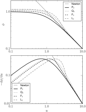
Figure 1: Top panel: the dimensionless interaction potential of the softening recipes listed in Table 1. Bottom panel: the corresponding interparticle forces. The dimensionless interaction potentials (top) and inter-particle forces (bottom) of these softening kernels are listed in Table 1. The kernels are scaled according to equations (19) and (20) to obtain a common maximum inter-particle force (as is obvious in the bottom panel), see also Section 2.3. Note that kernels with $a_{0}=0$ (Q₂ and L₂) have super-Newtonian gravity at intermediate scales to compensate for the sub-Newtonian behaviour at $r\to 0$.

The functional forms and other properties of the softening kernels used in this study are listed in Table 1. Their interparticle interaction potentials and forces are plotted in Figure 1. In particular, we list the dimensionless interparticle interaction potential $\phi$ and the corresponding three-dimensional and two-dimensional dimensionless density kernels, denoted by $\varrho$ and $\sigma$, respectively, assigned to each point particle.

In three dimensions, gravitational softening is equivalent to estimating the spatial mass density as a superposition of spheres with density distribution $\rho(r)$ placed at the particle positions. In two dimensions, one can consider softening as a way of smoothing the overall mass distribution as a superposition of razor-thin discs with density distribution $\Sigma(r)$ at the particle positions. For a softening kernel $\phi$, these spherical or razor-thin surface density distributions are given by

$$\rho(r)=\frac{m}{\varepsilon^{3}}\varrho\left(\frac{r}{\varepsilon}\right)\qquad\text{and}\qquad\Sigma(r)=\frac{m}{\varepsilon^{2}}\sigma\left(\frac{r}{\varepsilon}\right),$$ (11)

where the dimensionless density and surface-density kernels are given by

$$\varrho(u) =-\frac{1}{4\pi u^{2}}\frac{\mathrm{d}}{\mathrm{d}u}\left(u^{2}\frac{\mathrm{d}\phi}{\mathrm{d}u}\right),$$ (12a)

$$\sigma(u) =-\frac{1}{\pi^{2}}\int_{u}^{\infty}\frac{\mathrm{d}x\,}{\sqrt{x^{2}-u^{2}}}\frac{\mathrm{d}}{\mathrm{d}x}\int_{0}^{x}\frac{x\,\mathrm{d}t}{\sqrt{x^{2}-t^{2}}}\,\frac{\mathrm{d}\phi(t)}{\mathrm{d}t},$$ (12b)

respectively (Binney & Tremaine, 2008; Kalnajs, 1999).

Note that the softened force is that between a softened particle (with density distribution $\rho(r)$ or $\Sigma(r)$ given by eqn. (11)) and a point particle and not the force between two softened particles (Barnes, 2012). This remark applies to all softening techniques.

2.2.1 Plummer softening P₀: infinite support, $a_{0}\neq 0$

In three dimensions, this popular softening method corresponds to estimating the spatial mass density as a superposition of Plummer spheres (Plummer, 1911) with scale radius $\varepsilon$ at the particle positions. In two dimensions, Plummer softening amounts to smoothing the overall mass distribution as a superposition of razor-thin Kuz’min discs (Kuz’min, 1956).

Plummer softening modifies the gravitational interaction at all interparticle separations and asymptotes to the Newtonian interaction only for infinitely large particle separations. As a result, $a_{0}^{\mathrm{3D}}=\infty$ and the gravity bias (10) in this case grows faster than $\propto\varepsilon^{2}$. In two dimensions, this method’s non-zero $a_{0}$ indicates that the gravity bias increases linearly with softening length.

2.2.2 Modified Kuz’min softening Q₂: infinite support, $a_{0}=0$

One can modify the Plummer kernel such that $a_{0}$, $a_{2}$, …, $a_{k}=0$, for any chosen even $k$, in order to significantly reduce the gravity bias. For instance, we introduce the class of modified Kuz’min potentials, with an interaction potential given by

$$\phi(u)=\frac{K_{n}(u^{2})}{\left(1+u^{2}\right)^{n+1/2}},$$ (13)

here $K_{n}(u^{2})=\sum_{i=0}^{n}c_{i}u^{2i}$ is a polynomial of degree $n$ in $u^{2}$ with coefficients $c_{i}$. We refer to the $n^{\rm th}$ member of this class as Q_n. Clearly, the choice $n=0$ yields the Plummer kernel, or: Q₀=P₀.

The extra degree of freedom that comes with the choice $n=1$, can be exploited to make $a_{0}=0$. For instance, for this Q₁ kernel, one finds that

$$a_{0} \propto\lim_{x\rightarrow\infty}\int_{0}^{x}\left(1-\frac{c_{0}u+c_{1}u^{3}}{\left(1+u^{2}\right)^{3/2}}\right)\mathrm{d}u$$

$$=\lim_{x\rightarrow\infty}\left\{(1-c_{1})x+2c_{1}-c_{0}+{\cal O}\left(\frac{1}{x}\right)\right\}$$ (14)

and the choice $c_{0}=2$, $c_{1}=1$ makes $a_{0}=0$. Thus, the ‘Q₁’ method is defined by the interparticle potential

$$\phi(u)=\frac{2+u^{2}}{(1+u^{2})^{3/2}}$$ (15)

and by the corresponding 3D and 2D density distributions

$$\varrho(u)=\frac{3}{4\pi}\frac{4-u^{2}}{(1+u^{2})^{7/2}}\,\,\text{ and }\,\,\sigma(u)=\frac{3}{2\pi}\frac{1}{(1+u^{2})^{5/2}}.$$ (16)

In order to achieve $a_{0}=0$, this softening method compensates with slightly super-Newtonian forces at $r\apprge 1.2\varepsilon$ for the substantially sub-Newtonian accelerations at small separations. Unfortunately, while we now have $a_{0}=0$, the Q₁ softening kernel still has a diverging second-order coefficient $a_{2}$, such that the gravity bias grows faster than $\varepsilon^{3}$.

The extra degree of freedom provided by coefficient $c_{2}$ of kernel Q₂ can be used to provide $a_{2}$ with a finite value. Indeed, for this kernel, we find that

$$a_{0} \propto\lim_{x\rightarrow\infty}\int_{0}^{x}\left(1-\frac{c_{0}u+c_{1}u^{3}+c_{2}u^{5}}{\left(1+u^{2}\right)^{5/2}}\right)\mathrm{d}u$$

$$=\lim_{x\rightarrow\infty}\left\{(1-c_{2})x+\frac{1}{3}(8c_{2}-2c_{1}-c_{0})+{\cal O}\left(\frac{1}{x}\right)\right\}$$ (17)

and

$$a_{2} \propto\lim_{x\rightarrow\infty}\int_{0}^{x}\left(1-\frac{c_{0}u+c_{1}u^{3}+c_{2}u^{5}}{\left(1+u^{2}\right)^{5/2}}\right)u^{2}\mathrm{d}u$$

$$=\lim_{x\rightarrow\infty}\left\{\frac{1}{3}(1-c_{2})x^{3}+\left(\frac{5c_{2}}{2}-c_{1}\right)x\right.$$

$$\left.\hskip 80.00012pt-\frac{2}{3}(8c_{2}-4c_{1}+c_{0})+{\cal O}\left(\frac{1}{x}\right)\right\}.$$ (18)

Demanding $a_{0}$ to be zero and $a_{2}$ to be finite, leads to $c_{2}=1$, $c_{1}=5/2$, and $c_{0}=3$. All properties of this Q₂ kernel are listed in Table 1.

Of course, this game can be continued to obtain $a_{2}=0$, then finite $a_{4}$, then $a_{4}=0$, etc. However, the functional form of the resulting interaction potentials becomes increasingly complex.

2.2.3 Ferrers $n=3$ softening F₃: compact support, $a_{0}\neq 0$

An increasingly popular method is cubic spline softening, which in three-dimensional $N$-body simulations corresponds to replacing each particle by a cubic-spline smoothing kernel as is widely used in Smoothed Particle Hydrodynamics (SPH) codes (see e.g. Monaghan, 1992) and was introduced as a gravitational softening kernel for $N$-body/SPH codes by Hernquist & Katz (1989). Its main advantages in this context are its exactly Newtonian behaviour beyond the softening length and its dual use as hydrodynamics smoother and gravity softener. However, its interparticle potential and 3D density distribution are numerically rather unattractive due to their complex, piecewise continuous functional forms.

Here and in the remainder, we will use the phrase “compact support” to indicate that a kernel yields exactly Newtonian forces outside the softening kernel. In three dimensions, it immediately follows from Newton’s first theorem that the corresponding density distribution is zero outside the kernel, i.e. $\varrho=0$ at $u>1$. In two dimensions, this is not the case. In fact, all softening kernels with exact Newtonian gravity at separations $r>\varepsilon$ have poorly behaved corresponding razor-thin disc profiles $\sigma(u)$ (12b), with infinite spatial extent and negative values.

We here opt for the so-called Ferrers softening methods, labeled ‘F_n’, whose interaction potentials are polynomials of degree $n+1$ in the variable $t=1-u^{2}$ inside the softening length and that behave exactly Newtonian at separations $r>\varepsilon$. In three dimensions, they correspond to replacing each particle with a Ferrers (1877) sphere of order $n$. For $n=0$ this is just a homogeneous sphere. Higher-order models have spherical densities that are simple polynomials, with $n$ continuous derivatives, in the variable $t=1-u^{2}$.

For this paper, we investigate member $n=3$ from this family, with properties listed in Table 1, as an example of a softening method with compact support but with $a_{0}\neq 0$.

2.2.4 Modified Ferrers softening L₂: compact support, $a_{0}=0$

It is possible to modify the Ferrers softening methods to obtain $a_{0}=0$ in order to reduce their gravitational bias while retaining the attractive property of having compact support. Here, we test the method labeled ’L₂’, or ‘2D modified Ferrers $n=2$’, in Table 1. Its name derives from the fact that it’s based on the F₂ kernel, which has as an interaction potential $\phi(u)=1+\frac{1}{2}t+\frac{3}{8}t^{2}+\frac{5}{16}t^{3}$, but where the coefficient of the last term is tuned to make $a_{0}=0$. This leads to the L₂ interaction potential $\phi(u)=1+\frac{1}{2}t+\frac{3}{8}t^{2}+\frac{5}{2}t^{3}$.

This kernel achieves its desirable properties by having super-Newtonian accelerations for a limited range of separations close to and inside of $r=\varepsilon$.

2.3 Softening scale

The softening length and kernel are only defined up to a re-scaling: the softened potential (5) is invariant under the transformation

$$\varepsilon\to a\varepsilon\qquad\text{and}\qquad\phi(q)\to a\phi(aq)$$ (19)

with scaling factor $a$. This implies that the parameter $\varepsilon$ has no natural scale by itself and comparing different kernels at the same $\varepsilon$ is meaningless. Therefore, some other measure is required for such a comparison. One such measure valid for all softening kernels is the force-scaling as

$$\varepsilon_{F}=\varepsilon/\sqrt{-\phi^{\prime}_{\max}},$$ (20)

where $-\phi^{\prime}_{\max}$ denotes the maximum value of the derivative of $\phi$ (Springel, 2010). The ratios $\varepsilon_{F}/\varepsilon$, scaled to unity for the Plummer kernel, are listed in Table 1 for the kernels considered in this study.

For kernels with $a_{0}\neq 0$, another natural measure of the softening length is

$$\varepsilon_{0}\equiv\frac{a_{0}}{2\pi}\varepsilon=\int_{0}^{\infty}\left[1-r\psi(r)\right]\mathrm{d}r,$$ (21)

which measures the actual scale of the bias irrespective of any re-scaling. With this definition, $\varepsilon_{0}=\varepsilon$ for Plummer softening. For other softening methods used in this study, $\varepsilon_{0}$ is given in Table 1.

Likewise, softening techniques with zero $a_{0}$ but non-zero $a_{2}$ can be scaled to a common level of gravity bias via the softening length transformation

$$\varepsilon_{2}=\left|\frac{3a_{2}}{\pi}\right|^{1/3}\varepsilon.$$ (22)

With this definition, $\varepsilon=\varepsilon_{2}$ for Q₂ softening.

3 Softened gravity in stability analysis

3.1 Linear mode theory

We use pyStab, a Python/C++ computer code, to analyse the stability of a razor-thin stellar disc embedded in an axially symmetric gravitational potential. The details of the mathematical formalism behind this code and of its implementation can be found in Vauterin & Dejonghe (1996), Dury et al. (2008), and De Rijcke & Voulis (2016) so we will not repeat these here. An axially symmetric disc galaxy model is characterized by a distribution function $F_{0}(E,J)$, with $E$ the specific binding energy and $J$ the specific angular momentum of a stellar orbit, and a mean gravitational potential $V_{0}(r)$. In the remainder, we will refer to this unperturbed axially symmetric state as the “base state” of the system. Note that this base state is only a correct solution of the CBE when employing the Newtonian gravitational interaction (but see below).

For any given base state, pyStab can retrieve those complex frequencies $\omega$ for which a spiral-shaped perturbation of the form

$$V_{\rm pert}(r,\theta,t)=V_{\rm pert}(r)\,\mathrm{e}^{\mathrm{i}(m\theta-\omega t)}$$ (23)

constitutes an eigenmode. Here, $(r,\theta)$ are polar coordinates in the stellar disc, $m$ is the multiplicity of the spiral pattern, $\Omega_{p}=\Re\{\omega\}/m$ its pattern speed, and $\Im\{\omega\}$ its growth rate. A general perturbing potential can always be expanded in such modes and, owing to the linear approximation, these can be studied independently from each other.

In essence, pyStab solves the first-order CBE to find the response distribution function $f_{\rm resp}(r,\theta,v_{r},v_{\theta},t)$ produced by a given perturbation $V_{\rm pert}(r,\theta,t)$. This response distribution function generates the response density

$$\Sigma_{\rm resp}(r,\theta,t)=\int{f}_{\mathrm{resp}}(r,\theta,v_{r},v_{\theta},t)\,\mathrm{d}v_{r}\mathrm{d}v_{\theta}$$ (24)

which in turn gives rise to the response softened gravitational potential

$$V_{\rm resp}(\boldsymbol{x})=G\int\Sigma_{\rm resp}(\boldsymbol{x}^{\prime})\,\psi(|\boldsymbol{x}-\boldsymbol{x}^{\prime}|)\,\mathrm{d}^{2}\!\boldsymbol{x}^{\prime},$$ (25)

where the integral runs over the whole surface of the stellar disc and $\psi(r)$, defined in equation (4), is the softened Green’s function for gravitational interactions, replacing the Newtonian $1/r$. Eigenmodes are then identified by the fact that

$$V_{\rm pert}(r,\theta,t)\equiv V_{\rm resp}(r,\theta,t)$$ (26)

and pyStab employs a matrix method (Kalnajs, 1977) to find them. The perturbing potential $V_{\rm pert}$ is expanded in a basis of potentials, $V_{\ell}$. The response to each basis potential, denoted by $V_{\ell,\rm resp}$, can likewise be expanded in this basis as

$$V_{\ell,\rm resp}=\sum_{k}{\mathcal{C}}_{k\ell}V_{k}.$$ (27)

If the perturbation is an eigenmode, then the ${\mathcal{C}}$ matrix can be shown to possess a unity eigenvalue (Vauterin & Dejonghe, 1996; Dury et al., 2008; De Rijcke & Voulis, 2016). This feature is exploited by pyStab to identify the eigenmodes.

The formalism contains a number of technical parameters, such as the number of orbits on which phase space is sampled (here we use $n_{\rm orbit}(n_{\rm orbit}+1)/2$ orbits with $n_{\rm orbit}=600$ in the allowed triangle of turning point – or pericentre/apocentre – space), the number $n_{\rm Fourier}$ of Fourier components in which the periodic part of the perturbing potential is expanded (here we use $n_{\rm Fourier}=80$), the number of potential-density pairs (PDPs) that is used for the expansion of the radial part of the perturbing potential and density (we use 44 PDPs), and the shape and extent of the PDP density basis functions. As in De Rijcke & Voulis (2016), we use PDP densities of the form

$$\Sigma_{\ell}(r)=\Sigma_{0}(r)\exp\left(-\frac{1}{2}\left(\frac{r-r_{\ell}}{\sigma_{\ell}}\right)^{2}\right)$$ (28)

where the average radii $r_{\ell}$ cover the relevant part of the stellar disc and are evenly spaced on a logarithmic scale so the resolution is highest in the inner regions of the disc. The widths $\sigma_{\ell}$ are automatically chosen such that consecutive basis functions are sufficiently unresolved to represent any smooth function. The position of these PDP density basis functions can be tuned to achieve a high spatial resolution there where the eigenmodes live. The corresponding PDP potentials are obtained via

$$V_{\ell}(\boldsymbol{x})=G\int\Sigma_{\ell}(\boldsymbol{x}^{\prime})\,\psi(|\boldsymbol{x}-\boldsymbol{x}^{\prime}|)\,\mathrm{d}^{2}\!\boldsymbol{x}^{\prime}.$$ (29)

3.2 Introducing gravitational softening

Since we want to validate our approach by comparing particular results with published work based on numerical simulations, we mimic the strategies employed by simulators when setting up and performing $N$-body simulations of disc galaxies aimed at mode analysis. Usually, an initial condition is generated by sampling stellar particles from the distribution function $F_{0}(E,J)$ evaluated using the Newtonian gravitational potential $V_{0}(r)$, independent of the gravitational softening that is employed later on when evolving the particles through time. Moreover, the axially symmetric force field of the base state is subsequently evaluated correctly, i.e. without softening, either by directly using the analytical expression for the potential $V_{0}$ or by adding a small correction to the softened gravitational field derived from the particles. Only the non-axisymmetric force field of the growing waves is softened (Earn & Sellwood, 1995; Sellwood & Evans, 2001; Sellwood, 2012). This allows a simulator to sample particles from the correct DF evaluated in the correct potential so that at least the initial conditions of a simulation correspond to the intended base state and the particle dynamics in the axially symmetric force field is followed correctly.

Therefore, we only implement gravitational softening in the response potential $V_{\rm resp}(r,\theta,t)$, but not in the axially symmetric base state potential $V_{0}(r)$. Using this strategy, eqn. (25), and a fortiori eqn (29), is the only place where the softened gravitational interaction enters the computation of the modes. It is therefore straightforward to insert interaction potentials other than the Newtonian one into a mode analysis code. The gravity bias introduced in Section 2.1 must then be regarded as a measure for the fidelity with which the softened response potential resembles the Newtonian one. Thus, we can use linear stability theory to emulate the results expected in the large $N$ limit from $N$-body simulations of disc galaxies. In this paper, we investigate the effect on the eigenmodes in disc galaxy models from the P₀, Q₂, F₃, and L₂ softening methods listed in Table 1.

4 The base states

Below, we give the essential details of the two base states that we employ for this study. We also list the frequencies of the known eigenmodes of these base states computed for a Newtonian interparticle interaction.

4.1 The isochrone disc model

The isochrone disc is characterized by the cored density profile

$$\Sigma_{0}(r)=\frac{Mb}{2\pi r^{3}}\left(\ln\frac{r+\sqrt{r^{2}+b^{2}}}{b}-\frac{r}{b}\right)$$ (30)

which self-consistently generates the gravitational potential

$$V_{0}(r)=\frac{GM}{b+\sqrt{b^{2}+r^{2}}},$$ (31)

(Henon, 1959; Kalnajs, 1976). Here, $M$ is the total mass of the stellar disc and $b$ its scale-length. As shown by Kalnajs (1976) and Earn & Sellwood (1995), a family of distribution functions that generate this potential-density pair is given by

$$F_{0}(E,J)=\left[\frac{E}{V_{0}(0)}\right]^{{m_{K}}-1}g_{m_{K}}(x)$$ (32)

with $m_{K}$ an integer, $x=J\sqrt{2E}/GM$, and

$$g_{m_{K}}(x) =\frac{2^{m_{K}}}{2\pi V_{0}(0)}\Bigg{[}x\frac{\mathrm{d}\tau_{m_{K}}}{\mathrm{d}x}-\frac{{m_{K}}({m_{K}}-3)}{2}\tau_{m_{K}}(x)$$

$$\phantom{=\frac{2^{m_{K}}}{2\pi V_{0}(0)}\Bigg{[}}+\int_{0}^{1}\tau_{m_{K}}(\eta x)\,\eta^{m_{K}}\frac{\mathrm{d}^{2}P_{{m_{K}}-1}}{\mathrm{d}\eta^{2}}\mathrm{d}\eta\Bigg{]}.$$ (33)

Here, $P_{m}$ is the Legendre polynomial of degree $m$ and

$$\tau_{m_{K}}(x) =-\frac{M}{16\pi b^{2}}\frac{(1-x^{2})^{3-{m_{K}}}}{x^{3}(1+x^{2})}$$

$$\hskip 40.00006pt\times\left[2x+(1+x^{2})\ln\frac{1-x}{1+x}\right].$$ (34)

We adopt $m_{K}=12$ for this study. The Legendre polynomial can be evaluated explicitly, allowing the integral featuring in the expression for the distribution function to be evaluated in closed form. However, the resulting expression is numerically very unstable for small $x$. Therefore, we opted to simply evaluate the integral numerically. This distribution function is only used to populate orbits with positive angular momentum.

Counter-rotating stars have been added according to the prescription given in Earn & Sellwood (1995) which, unfortunately, necessitates going back and forth between energy, angular momentum and the radial action variable, $J_{r}$:

$$F^{\prime}_{0}(E,J)=\left\{\begin{array}[]{ll}\frac{1}{2}F_{0}(E^{\prime},0)&\text{if $J<0$}\\[4.30554pt] F_{0}(E,J)-\frac{1}{2}F_{0}(E^{\prime},0)&\text{if $J>0$}\end{array}\right.$$ (35)

with $E^{\prime}$ the energy corresponding to a radial action $J_{r}+|J|$ and zero angular momentum. Fortunately, analytical conversion formulæ between energy, angular momentum, and radial action exist for the isochrone disc (Binney & Tremaine, 2008).

We will focus here on the bisymmetric ($m=2$) modes of this model. Pichon & Cannon (1997) provide the frequencies of three modes of this base state model, choosing units such that $G=M=b=1$, as

$$\begin{array}[]{r@{=}r@{\,+\,}r@{\,\mathrm{i}}}\omega_{1}&0.59&0.21\\[2.15277pt] \omega_{2}&0.46&0.14\\[2.15277pt] \omega_{3}&0.26&0.05\end{array}$$ (36)

while Jalali & Hunter (2005) find

$$\begin{array}[]{r@{=}r@{\,+\,}r@{\,\mathrm{i}}}\omega_{1}&0.584&0.217\\[2.15277pt] \omega_{2}&0.468&0.148\end{array}$$ (37)

for the two main modes.

4.2 The Mestel disc

The Mestel (1963) disc has a cusped total surface density given by

$$\Sigma_{0}(r)=\Sigma_{0}\frac{r_{0}}{r}$$ (38)

which self-consistently generates a gravitational potential of the form

$$V_{0}(r)=-v_{0}^{2}\ln\left(\frac{r}{r_{0}}\right)$$ (39)

with the surface density scale given by $\Sigma_{0}=v_{0}^{2}/2\pi Gr_{0}$. Here, $v_{0}$ is the value of the disc’s constant circular velocity. A central hole is cut out of this disc model by multiplying its distribution function (Toomre, 1977)

$$f(E,J)=\frac{\Sigma_{0}v_{0}^{q}}{\sqrt{2^{q}\pi}\Gamma\left(\frac{q+1}{2}\right)\sigma^{q+2}}\left(\frac{J}{r_{0}v_{0}}\right)^{q}\mathrm{e}^{E/\sigma^{2}},$$ (40)

where $q$ is a real number, with a cut-out function of the form

$$H_{\rm cut}(J)=\frac{x}{1+x}$$ (41)

with $x=\left(J/r_{0}v_{0}\right)^{n}$ (obviously, this also slightly suppresses the distribution function at larger $J$-values). Outside the central cut-out region, the disc’s constant radial velocity dispersion is given by $\sigma=v_{0}/\sqrt{1+q}$.

Here, we will focus on the $q=6$, $n=4$ member of this model family and adopt units such that $G=v_{0}=r_{0}=1$. Its dominant bisymmetric mode is then expected to have a frequency

$$\omega_{1}\approx 0.88+0.13\,\mathrm{i},$$ (42)

as shown, e.g., by Toomre (1977); Read (1997); Evans & Read (1998); Polyachenko & Just (2015). This mode owes its existence to the inner cutout: if the angular momentum cut-off is not sufficiently steep, i.e. if $n$ is too small, there is no eigenmode. The idea is that incoming trailing wave packets are (partially) reflected from this sharp inner edge to travel back outwards as leading waves. Overreflection, or swing amplification, at the evanescent zone around the corotation resonance (Mark, 1976; Toomre, 1981) sends amplified trailing waves back inwards. Inside this resonance cavity, growing modes can occur (Evans & Read, 1998).

5 Results

5.1 The isochrone disc

5.1.1 Unsoftened gravity

For the two most rapidly growing $m=2$ modes of the $m_{K}=12$ isochrone disc, we find frequencies

$$\omega_{1} =0.582+0.215\;\mathrm{i}$$ (43)

$$\omega_{2} =0.466+0.146\;\mathrm{i},$$

in good agreement with published values.

However, the third mode listed by Pichon & Cannon (1997) showed up in our analysis as only the fifth fastest growing mode, with a frequency

$$\begin{array}[]{r@{=}r@{\,+\,}r@{\;\mathrm{i}}}\omega_{3}&0.272&0.053\end{array}.$$ (44)

The two interloping modes at

$$\begin{array}[]{r@{=}r@{\,+\,}r@{\;\mathrm{i}}}\omega^{\prime}_{3}&0.384&0.103\\[2.15277pt] \omega^{\prime}_{4}&0.323&0.075\end{array}$$ (45)

have not been described in the literature before. We confirmed that they are robust to changes of the numerical parameters in the code (resolution in phase space, number of Fourier modes, etc.) and that they exert a zero total torque on the disc, as they should, and therefore see no reason to discard them as spurious (Polyachenko & Just, 2015).

5.1.2 Softened gravity

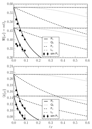
Figure 2: Pattern speeds $\Re\{\omega\}=m\Omega_{p}$ (top panel) and growth rates $\Im\{\omega\}$ (bottom panel) of the two dominant $m=2$ modes of the $m_{K}=12$ isochrone disc, with unsoftened frequencies of $\omega_{1}=0.582+0.215\,{{\,\mathrm{i}}}$ and $\omega_{2}=0.466+0.146\,{{\,\mathrm{i}}}$ for different softening recipes (Plummer P₀, modified Kuz’min Q₂, Ferrers F₃, and modified Ferrers L₂). The softening lengths are scaled according to equations (19) and (20) to obtain a common maximum inter-particle force. The bullets are data taken from the $N$-body simulations using Plummer softening reported in Earn & Sellwood (1995). The horizontal grey lines indicate the Newtonian mode frequency.

For this base state, published information on how the properties of the two main $m=2$ modes change with softening in a numerical simulation exists. Earn & Sellwood (1995) use a polar grid code with 120,000 particles, a fixed time step, and a polar grid of 128 azimuthal and 85 radial nodes to simulate the $m_{K}=12$ isochrone disc from quiet-start initial conditions (Sellwood, 1983) using Plummer softening with different softening lengths. The results of these simulations are shown in Fig. 2 as black data points. Both the pattern speed and the growth rate of the two dominant modes appear to be declining functions of softening length. As Earn & Sellwood (1995) note: “[…] it is clear that both parts of the eigenfrequency are strongly affected by even moderate softening.” The dependence of the mode frequencies on softening length is markedly non-linear which hampers a simple extrapolation to zero softening length.

Overplotted in Fig. 2 are the results from our linear stability analysis with pyStab, using different softening prescriptions. Clearly, our results for Plummer softening agree rather well with those presented in Earn & Sellwood (1995): both the pattern speed and growth rate are non-linearly declining functions of the softening length (scaled according to equations (19) and (20) to a common maximum inter-particle force). The drop is steepest for small softening lengths and becomes shallower for larger $\varepsilon$. Especially for larger $\varepsilon$-values, numerical simulations and linear mode analysis predict the same behaviour for frequency as a function of softening length. We tentatively attribute the deviations between the simulations and linear theory at small $\varepsilon$-values to variance, i.e. to the gravity error caused by not softening enough (cf. paragraph 2.1).

Using the other softening recipes, the pattern speed and growth rate likewise decline with increasing softening length but they do so much less dramatically and with smaller deviation from a linear dependence on softening length than when using Plummer softening. Moreover, it appears that having a zero gravity bias parameter $a_{0}$ induces a much stronger effect than having compact support. This is exemplified in this case by the Q₂ method (infinite support, $a_{0}=0$) yielding results much closer to the Newtonian ones than the F₃ method (compact support, $a_{0}>0$). Methods that combine compact support with having $a_{0}=0$, like the L₂ method, appear vastly superior, with very little deviation between the retrieved mode frequencies and the correct, Newtonian values.

However, we refer the reader to section 6 for a discussion of how to correctly interpret this apparent success.

5.2 The Mestel disc

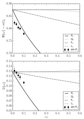
Figure 3: Pattern speed $\Re\{\omega\}=m\Omega_{p}$ (top panel) and growth rate $\Im\{\omega\}$ (bottom panel) of the dominant $m=2$ mode of the $q=6$, $n=4$ Mestel disc for different softening recipes (Plummer P₀, modified Kuz’min Q₂, Ferrers F₃, and modified Ferrers L₂). The softening lengths are scaled according to equations (19) and (20) to obtain a common maximum inter-particle force. The datapoints are derived from the $N$-body simulations by Sellwood & Evans (2001). The horizontal grey lines indicate the Newtonian mode frequency.

5.2.1 Unsoftened gravity

pyStab retrieves the dominant mode of the $q=6$, $n=4$ Mestel disc, along with a number of much slower growing modes. Since the frequencies of these minor modes are sensitive to the choice of numerical parameter values, they are most likely spurious (Polyachenko & Just, 2015). Using unsoftened gravity, we find the dominant mode to have a frequency $\omega=0.876+0.128\;\mathrm{i}$, which is in good agreement with the values reported by Toomre (1977); Read (1997); Polyachenko & Just (2015) and which were computed using different mode analysis techniques and codes.

5.2.2 Softened gravity

In Fig. 3, we show how the pattern speed (top panel) and growth rate (bottom panel) of the dominant mode of this base state change with increasing softening length (scaled according to equations (19) and (20) to a common maximum inter-particle force) using the softening recipes listed in Table 1.

Overplotted in this figure, we show the frequency estimates of Sellwood & Evans (2001) for this Mestel disc model, based on $N$-body simulations with a particle-mesh code employing 2.5 million particles, and a grid of 256 azimuthal and 200 radial nodes. The 5 simulations presented here all start from exactly the same initial conditions but are evolved using different Plummer softening lengths. The agreement with our linear mode analysis is not as good as in the case of the isochrone disc. As reported by Sellwood & Evans (2001), there is a $\sim 10$ % scatter between the measured frequencies of simulations with resampled initial conditions at a constant particle number. This may be why the simulation datapoints do not converge to the Newtonian linear-mode result for zero softening length. Moreover, particle noise may have negatively affected the frequency measurements. Still, the trend followed by these simulations is in qualitative agreement with our results: both the pattern speed and the growth rate decrease with increasing softening length.

As for the isochrone disc, softening methods with $a_{0}=0$ (like Q₂) stay much closer to the Newtonian mode frequency than methods with compact support but non-zero $a_{0}$ (like F₃) for a given value of the softening length $\varepsilon$. Methods that combine compact support with $a_{0}=0$ (like L₂) generally outperform the others.

Again, we refer the reader to section 6 for a discussion of how to correctly interpret this apparent success.

6 Discussion

6.1 Scaling to the same level of gravity bias

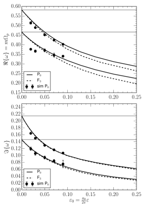
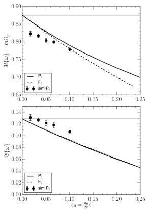
Figure 4: Pattern speed $\Re\{\omega\}=m\Omega_{p}$ (top panels) and growth rate $\Im\{\omega\}$ (bottom panels) of the dominant $m=2$ mode of the $m_{K}=12$ isochrone disc (left panels) and the $q=6$, $n=4$ Mestel disc (right panels) as a function of the scaled softening length $\varepsilon_{0}$, which allows for a direct comparison of the softening kernels with non-zero $a_{0}$ (i.e. P₀ and F₃) at the same level of gravity bias. The bullets are data taken from the $N$-body simulations using Plummer softening reported in Earn & Sellwood (1995) and Sellwood & Evans (2001). The horizontal grey lines indicate the Newtonian mode frequencies.

As mentioned in paragraph 2.3, the softening length and kernel are only defined up to a re-scaling and we advocate the scale

$$\varepsilon_{0}=\frac{a_{0}}{2\pi}\varepsilon$$ (46)

to bring methods with non-zero $a_{0}$ to a common gravity bias level.

In Fig. 4, we show the retrieved frequencies of the modes of the isochrone and Mestel discs as a function of $\varepsilon_{0}$ for the two softening methods with non-zero gravity bias parameter $a_{0}$ (i.e. P₀ and F₃). Clearly, the differences between both softening methods, which are so striking in Figures 2 and 3, now largely disappear. At a given $\varepsilon_{0}$-value, all $a_{0}\neq 0$ methods perform almost equally well. Thus, it is always possible to re-scale the softening length of one $a_{0}\neq 0$ softening technique such that it approximately matches the performance of another $a_{0}\neq 0$ method. No exact matching is possible because of the higher order terms in the expansion of the gravity bias.

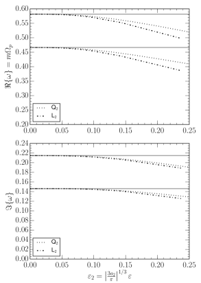
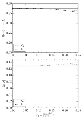
Figure 5: Pattern speed $\Re\{\omega\}=m\Omega_{p}$ (top panels) and growth rate $\Im\{\omega\}$ (bottom panels) of the dominant $m=2$ mode of the $m_{K}=12$ isochrone disc (left panels) and the $q=6$, $n=4$ Mestel disc (right panels) as a function of the scaled softening length $\varepsilon_{2}$, which allows for a direct comparison of the softening kernels with zero $a_{0}$ (i.e. Q₂ and L₂) at the same level of gravity bias. The horizontal grey lines indicate the Newtonian mode frequencies.

As can be seen in Figure 5, softening techniques with $a_{0}=0$ but non-zero $a_{2}$ can be scaled to a common level of gravity bias using the transformation (22), allowing for higher order terms in the expansion (8) for the gravity bias.

Based on these results, it seems fair to say that softening strategies with $a_{0}=0$ generally yield more accurate (i.e. Newtonian-like) mode frequencies than strategies with $a_{0}\neq 0$ because the gravity bias of the latter grows linearly with softening length $\varepsilon$ while for the former it grows much more slowly, as $\varepsilon^{3}$. However, within each of these classes of softening techniques, there is no particular reason to favour one method over another provided they are compared at (approximately) the same level of gravity bias.

6.2 Physical interpretation

We define the two-dimensional Fourier transform $\widehat{\psi}(k)$ of the interparticle interaction potential $\psi(r)$ as

$$\psi(\boldsymbol{r})=\frac{1}{(2\pi)^{2}}\int\widehat{\psi}(k){{\,\mathrm{e}}}^{{{\,\mathrm{i}}}\boldsymbol{k}.\boldsymbol{r}}\mathrm{d}\boldsymbol{k}.$$ (47)

Based on Poisson’s equation, using separation of variables it is straightforward to show that the radial part of the gravitational response potential, which we denote here by $V_{m}(r)$, generated by an $m$-armed spiral response density of the form

$$\Sigma_{m}(r,\theta)=\Sigma_{m}(r){{\,\mathrm{e}}}^{{{\,\mathrm{i}}}m\theta}$$ (48)

can be retrieved from the relation

$${\mathcal{H}}_{m}\left\{V_{m}(r)\right\}=-G\widehat{\psi}(k){\mathcal{H}}_{m}\left\{\Sigma_{m}(r)\right\}$$ (49)

with ${\mathcal{H}}_{m}$ the Hankel transform of order $m$ (see e.g. Binney & Tremaine, 2008). The Hankel transform of order $m$ of a function $f(r)$ is defined as

$${\mathcal{H}}_{m}\left\{f\right\}(k)=\int_{0}^{\infty}f(r)J_{m}(kr)r\mathrm{d}r$$ (50)

with $J_{m}(x)$ a Bessel function of the first kind.

Here, we will use the notation $\widehat{\psi}_{N}(k)$ for the Fourier transform of the Newtonian interaction potential, with

$$\widehat{\psi}_{N}(k)=\frac{2\pi}{k}.$$ (51)

Likewise, for the interaction potentials listed in Table 1 we find that:

$$\widehat{\psi}_{P_{0}}(k) =2\pi\frac{{{\,\mathrm{e}}}^{-k\varepsilon}}{k}$$ (52)

$$\widehat{\psi}_{Q_{2}}(k) =2\pi\left(1+k\varepsilon+\frac{1}{2}(k\varepsilon)^{2}\right)\frac{{{\,\mathrm{e}}}^{-k\varepsilon}}{k}.$$ (53)

For the softening techniques with compact support, F₃ and L₂, no simple analytical expression exists for the Fourier transform of their interaction potentials but they can easily be obtained numerically.

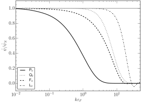
Figure 6: The suppression factor $\widehat{\psi}/\widehat{\psi}_{N}$ as a function of the dimensionless wave number $k\varepsilon_{F}$, where the softening lengths are scaled according to equations (19) and (20) to obtain a common maximum inter-particle force.

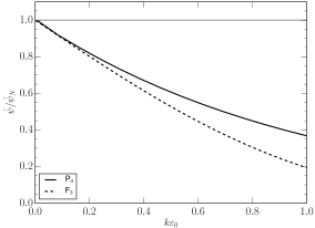
Figure 7: The suppression factor $\widehat{\psi}/\widehat{\psi}_{N}$ as a function of the re-scaled dimensionless wave numbers $k\varepsilon_{0}$ (top panel), for the softening methods with $a_{0}\neq 0$, and $k\varepsilon_{2}$ (bottom panel), for the softening methods with $a_{0}=0$.

For a given response density $\Sigma_{m}$, the softened response potential $V_{m}^{\varepsilon}$ and the unsoftened response potential $V_{m}^{0}$ are connected as

$${\mathcal{H}}_{m}\left\{V_{m}^{\varepsilon}\right\}=\frac{\widehat{\psi}}{\widehat{\psi}_{N}}{\mathcal{H}}_{m}\left\{V_{m}^{0}\right\}$$ (54)

with $\varepsilon$ the softening length. We plot the $k$-dependent suppression factor $\widehat{\psi}/\widehat{\psi}_{N}$ that links the Fourier transforms of the softened and unsoftened response potentials in Figure 6. The most striking consequence of gravitational softening is the suppression of the small-scale, i.e. large wavenumber $k$, structure in the Fourier transform of the response potential.

In Appendix A, we show how this suppression factor is connected to the gravity bias. More specifically, we prove that the even coefficients in the series expansion of the suppression factor around zero $k$ are directly proportional to the even coefficients in the series expansion of the gravity bias around zero $\varepsilon$ (in case the latter exist). Clearly, desiging a softening kernel to have vanishing bias coefficients is equivalent to designing an interaction kernel whose suppression factor $\widehat{\psi}/\widehat{\psi}_{N}$ is increasingly close to unity for small wavenumbers $k$.

However, just as it is not sensible to compare the various softening strategies as we did in Figures 2 and 3, it makes little sense to compare the suppression factors as a function of $k\varepsilon_{F}$. It is more meaningful to compare the suppression factors at the same level of gravity bias, i.e. as a function of $k\varepsilon_{0}$ for the softening methods with $a_{0}\neq 0$, and as a function of $k\varepsilon_{2}$ for the softening methods with $a_{0}=0$. This comparison is shown in Figure 7 and restates our previous conclusions. As a function of the re-scaled wave number $k\varepsilon_{0}$, which places the P₀ and F₃ kernels on an equal gravity bias footing, the suppression factors of these two softening techniques behave remarkably similar. In fact, Plummer softening leads to less suppression for large $k\varepsilon_{0}$ than F₃ softening. This agrees with Figure 4 in which Plummer softening is shown to stay closer to the correct, Newtonian result than F₃ softening at an equal level of gravity bias. The Q₂ kernel, in turn, leads to less suppression than the L₂ kernel and, as can be seen in Figure 5, it also leads to slightly better frequency estimates.

This suppression of the response potential will likely lead to an increased stability of the model galaxy. This expectation is borne out by studying the stability of axially symmetric WKBJ waves under Plummer softening, where a Toomre $Q$-value $Q<1$ now separates growing from stationary waves (Miller, 1971). This analysis has been extended to include general softening kernels by Romeo (1994, 1997). The physical background of our results and the expected influence of softening on $m=0$ WKBJ waves are, therefore, already well understood. Here, we took this work further by studying general eigenmodes beyond the WKBJ approximation and by going to $m=2$ patterns.

7 Conclusions

We use linear perturbation theory to investigate how different recipes for gravitational softening, as employed in numerical $N$-body simulations of razor-thin disc galaxies, affect predictions for the properties of the latter’s spiral eigenmodes. We specifically focus on the frequencies, i.e. pattern speeds and growth rates, of two-armed modes in the linear regime. We warn the reader that our approach does not take into account the effects of approximate force evaluations (Barnes & Hut, 1986), finite-$N$ (Dehnen, 2001; Sellwood, 2012; Fouvry et al., 2015), stochasticity (Sellwood & Debattista, 2009), implicit softening contributed by the grid in particle-mesh codes (Romeo, 1994), etc. whose respective magnitudes, moreover, may depend on the amount of gravitational softening.

We have tested our linear mode analysis approach by comparing the behaviour of the frequencies of the dominant $m=2$ modes of an isochrone disc and of the Mestel disc as a function of Plummer softening length with those found in the $N$-body simulations reported by Earn & Sellwood (1995) and Sellwood & Evans (2001). Overall, we found reasonably good agreement between linear theory and numerical simulations, also in the softened regime.

We argue that the only meaningful way of comparing softening kernels is to scale them to the same gravity bias level. In this paper, we show how this scaling can be achieved, based on the results of Dehnen (2001). Thus, it is always possible to re-scale the softening length of one softening technique such that it matches the performance of another method with the same dependence of gravity bias on softening length.

We have shown that softening methods with a vanishing lowest-order term in the expansion of the gravity bias as a function of softening length (in two dimensions, this is a linear term; in three dimensions, this term is quadratic in the softening length) and whose gravity bias therefore grows slowly with increasing softening length (e.g. the Q₂ and L₂ methods discussed in this paper) provide more accurate mode frequency estimates than methods with a non-zero lowest-order term (e.g. the P₀ and F₃ methods). Softening methods with zero lowest-order term compensate the sub-Newtonian forces deep inside the kernel with super-Newtonian forces near $r\sim\varepsilon$.

Kernels with compact support, in the sense that they yield exactly Newtonian forces outside of the softening kernel, perhaps somewhat counter-intuitively, do not necessarily provide more accurate frequency estimates than kernels with infinite extent. For instance, when compared at a common level of gravity bias, the Plummer kernel (P₀) provides more accurate frequency estimates than the F₃ kernel. Likewise, the Q₂ kernel outperforms the L₂ kernel in this regard.

The relative merit of a softening kernel can be judged from its suppression of the small-scale, i.e. large wavenumber $k$, structure in the Fourier transform of its response potential. The stronger this suppression, measured at a given level of gravity bias, the more the mode frequency estimates deviate from their Newtonian values.

As a guide to simulators, we provide an example of how a softening technique, in this case Plummer softening, can be used as a basis for developing new softening kernels whose gravity biases grow more slowly with increasing softening length. These then provide much more accurate estimates for mode frequencies than Plummer softening does.

Generally, the use of gravitational softening lowers the exponential growth rate of spiral modes. Therefore, strongly softened $N$-body simulations may risk “losing” some of these modes as their growth rates are overtaken by that of e.g. swing amplified noise (Romeo, 1995).

Appendix A The gravity bias and the suppression factor

A.1 Gravity bias

Analogous to the three-dimensional case discussed in Dehnen (2001), in two dimensions, the expectation value of the gravitational potential is

$$\left\langle\hat{V}(\boldsymbol{r})\right\rangle =-G\int\Sigma(\boldsymbol{r}^{\prime})\,\psi(|\boldsymbol{r}-\boldsymbol{r}^{\prime}|)\,\mathrm{d}^{2}\boldsymbol{r}^{\prime},$$ (55)

with $\Sigma$ the surface density that causes the gravitational potential $V$ through the inter-particle interaction potential $-\psi$. The integral covers the whole surface of the galaxy. The gravity bias can be obtained by rewriting the interaction potential as

$$\psi(r)=\frac{1}{\varepsilon}\phi\left(\frac{r}{\varepsilon}\right)=\frac{1}{r}-\frac{1}{\varepsilon}\left[\frac{\varepsilon}{r}-\phi\left(\frac{r}{\varepsilon}\right)\right],$$ (56)

which leads to

$$\mathrm{bias}_{\boldsymbol{r}}(\hat{V}) \equiv\left\langle\hat{V}(\boldsymbol{r})\right\rangle-V(\boldsymbol{r})$$

$$=\varepsilon G\int\Sigma(\boldsymbol{r}-\varepsilon\boldsymbol{u})\left[\frac{1}{u}-\phi(u)\right]\mathrm{d}^{2}\boldsymbol{u},$$ (57)

with $\varepsilon\boldsymbol{u}=\boldsymbol{r}-\boldsymbol{r}^{\prime}$. We replace the surface density by its Taylor expansion around the position $\boldsymbol{r}$,

$$\Sigma(\boldsymbol{r}-\varepsilon\boldsymbol{u})=\sum_{n=0}^{\infty}\frac{(-\varepsilon)^{n}}{n!}\left(\boldsymbol{u}.\boldsymbol{\nabla}\right)^{n}\Sigma(\boldsymbol{r}).$$ (58)

such that

$$\mathrm{bias}_{\boldsymbol{r}}(V) =\varepsilon G\sum_{n=0}^{\infty}\frac{(-\varepsilon)^{n}}{n!}\int\left[\frac{1}{u}-\phi(u)\right](\boldsymbol{u}\cdot\boldsymbol{\nabla})^{n}\Sigma(\boldsymbol{r})\,\mathrm{d}^{2}\boldsymbol{u}.$$ (59)

If we perform the integration in polar coordinates $(u,\theta)$ and replace $(\boldsymbol{u}\cdot\boldsymbol{\nabla})^{n}=u^{n}(\cos\theta\,\nabla_{\!x}+\sin\theta\,\nabla_{\!y})^{n}$ by its binomial expansion, we have

$$\mathrm{bias}_{\boldsymbol{r}}(V) =\varepsilon\,G\sum_{n=0}^{\infty}\frac{(-\varepsilon)^{n}}{n!}\int_{0}^{\infty}u^{n}\left[1-u\phi(u)\right]\,\mathrm{d}u$$

$$\phantom{=}\times\sum_{l=0}^{n}\binom{n}{l}\nabla_{\!x}^{l}\nabla_{\!y}^{n-l}\Sigma(\boldsymbol{r})\int_{0}^{2\pi}\cos^{l}\theta\sin^{n-l}\theta\,\mathrm{d}\theta.$$ (60)

The $\theta$ integral vanishes for odd $n$ or $l$, while for even $n$ and $l$

$$\int_{0}^{2\pi}\cos^{l}\theta\sin^{n-l}\theta\,\mathrm{d}\theta =\frac{2\pi n!}{2^{n}([n/2]!)^{2}}\binom{n/2}{l/2}\binom{n}{l}^{-1},$$ (61)

such that we obtain (using $\Delta\equiv\boldsymbol{\nabla}^{2}$)

$$\mathrm{bias}_{\boldsymbol{r}}(V) =\sum_{k=0}^{\infty}\varepsilon^{2k+1}a_{2k}\,G\,\Delta^{k}\Sigma(\boldsymbol{r})$$ (62)

with coefficients $a_{n}$ as given by equation (9).

A.2 Relation to the reduction factor

Because $f(\boldsymbol{r})\equiv r^{-1}-\psi(r)$ is an isotropic function in $\boldsymbol{r}$ space, its moments

$$\mu_{l,m}\equiv\int x^{l}\,y^{m}\,f(\boldsymbol{r})\,d^{2}\!\boldsymbol{r}$$ (63)

vanish for odd $l$ or $m$. For even $l$ and $m$,

$$\mu_{l,m} =\varepsilon^{n+1}\,a_{n}n!\binom{n/2}{l/2}\binom{n}{l}^{-1},$$ (64)

where $n=l+m$ and we have used relation (61). Let

$$F(\boldsymbol{k})\equiv\int f(\boldsymbol{r})\,\mathrm{e}^{-i\boldsymbol{k}\cdot\boldsymbol{r}}\,\mathrm{d}^{2}\!\boldsymbol{r}$$ (65)

be the two-dimensional Fourier transform of $f(\boldsymbol{r})$. Because $f(\boldsymbol{r})$ is isotropic and real-valued, then so is $F(\boldsymbol{k})=F(k)$. From the equation (65)

$$\left.\frac{\partial^{l+m}F}{\partial k_{x}^{l}\,\partial k_{y}^{m}}\right|_{\boldsymbol{k}=0} =(-i)^{l+m}\mu_{l,m},$$ (66)

and hence the Taylor expansion of $F(\boldsymbol{k})$

$$F(\boldsymbol{k}) =\sum_{l,m=0}^{\infty}\frac{k_{x}^{l}\,k_{y}^{m}}{l!\,m!}(-i)^{l+m}\mu_{l,m}=\varepsilon\sum_{\nu=0}^{\infty}(-1)^{\nu}\,a_{2\nu}\,|\varepsilon\boldsymbol{k}|^{2\nu}.$$ (67)

The reduction factor is related to $F(\boldsymbol{k})$ via

$$R(k)\equiv\widehat{\psi}(k)/\widehat{\psi}_{N}(k) =1-(2\pi)^{-1}kF(k).$$ (68)

Thus, the coefficients $c_{n}$ of the Taylor series

$$R(k)=1-\sum_{n=0}^{\infty}c_{n}\,(\varepsilon k)^{n+1}$$ (69)

are given by

$$c_{n}=(-1)^{n/2}a_{n}/2\pi$$ (70)

for even $n$ and if $a_{n}$ is finite. For odd $n$ and/or infinite $a_{n}$, the situation is more complicated. If the kernel $\psi$ has compact support or $\psi\sim r^{-1}$ exponentially fast as $r\to\infty$, then all the coefficients $a_{n}$ are finite, the Taylor series (67) of $F(\boldsymbol{k})$ converges, and relation (70) holds for all $n$, i.e. $R(k)$ is a function of $k^{2}$ only. This is the situation for the $F_{3}$ and $L_{2}$ kernels.

If the kernel does not satisfy the above conditions, but $f(r)\sim r^{-p}$ at $r\to\infty$, then $a_{n}=\infty$ for $n\geq p-2$ and the Taylor series (67) does not converge. However, the series of the non-divergent terms is still useful, only the remainder grows faster than $\varepsilon^{p-2}$. A typical example is Plummer softening, for which $a_{0}=2\pi$, while $a_{n>0}=\infty$ and (see equation 52)

$$F(\boldsymbol{k})=2\pi k^{-1}(1-\mathrm{e}^{-\varepsilon k})=2\pi\left[\varepsilon-\tfrac{1}{2}\varepsilon^{2}k\ldots\right],$$ (71)

i.e. $c_{0}=a_{0}/2\pi$ as per relation (70), but $c_{1}=-\tfrac{1}{2}\neq 0$. The problem is that the two-dimensional Fourier transform (71) is not smooth at the origin, but has discontinuous gradient (such that its Taylor series fails), while the one-dimensional function $F(k)$ and hence the reduction factor $R(k)$ are well behaved for all $k\geq 0$. Thus, a divergent $a_{n}$ indicates a non-vanishing $c_{n-1}$ and, conversely, a $c_{n-1}\neq 0$ for even $n$ implies $a_{n}=\infty$.

References

- Barnes & Hut (1986) Barnes J., Hut P., 1986, Nature, 324, 446
- Barnes (2012) Barnes J. E., 2012, Mon. Not. R. Astron. Soc., 425, 1104
- Binney & Tremaine (2008) Binney J., Tremaine S., 2008, Galactic Dynamics, second edition. Princeton University Press
- Colombi et al. (2015) Colombi S., Sousbie T., Peirani S., Plum G., Suto Y., 2015, Mon. Not. R. Astron. Soc., 450, 3724
- De Rijcke & Voulis (2016) De Rijcke S., Voulis I., 2016, Mon. Not. R. Astron. Soc., 456, 2024
- Dehnen (2001) Dehnen W., 2001, Mon. Not. R. Astron. Soc., 324, 273
- D’Onghia, Vogelsberger & Hernquist (2013) D’Onghia E., Vogelsberger M., Hernquist L., 2013, Astrophys. J., 766, 34
- Dury et al. (2008) Dury V., De Rijcke S., Debattista V. P., Dejonghe H., 2008, Mon. Not. R. Astron. Soc., 387, 2
- Earn & Sellwood (1995) Earn D. J. D., Sellwood J. A., 1995, Astrophys. J., 451, 533
- Evans & Read (1998) Evans N. W., Read J. C. A., 1998, Mon. Not. R. Astron. Soc., 300, 106
- Ferrers (1877) Ferrers N. M., 1877, Q. J. Pure Appl. Math., 14, 1
- Fouvry et al. (2015) Fouvry J. B., Pichon C., Magorrian J., Chavanis P. H., 2015, Astron. & Astrophys., 584, A129
- Fridman & Polyachenko (1984) Fridman A. M., Polyachenko V. L., 1984, Physics of Gravitating Systems - I. Equilibrium and Stability. Springer-Verlag
- Henon (1959) Henon M., 1959, Annales d’Astrophysique, 22, 126
- Hernquist & Katz (1989) Hernquist L., Katz N., 1989, Astrophys. J. Suppl., 70, 419
- Hohl (1971) Hohl F., 1971, Astrophys. J., 168, 343
- Jalali (2007) Jalali M. A., 2007, Astrophys. J., 669, 218
- Jalali & Hunter (2005) Jalali M. A., Hunter C., 2005, Astrophys. J., 630, 804
- Kalnajs (1976) Kalnajs A. J., 1976, Astrophys. J., 205, 751
- Kalnajs (1977) Kalnajs A. J., 1977, Astrophys. J., 212, 637
- Kalnajs (1999) Kalnajs A. J., 1999, in Astronomical Society of the Pacific Conference Series, Vol. 165, The Third Stromlo Symposium: The Galactic Halo, Gibson B. K., Axelrod R. S., Putman M. E., eds., p. 325
- Kuz’min (1956) Kuz’min G. G., 1956, Astr. Zh., 33, 27
- Mark (1976) Mark J. W. K., 1976, Astrophys. J., 205, 363
- Merritt (1996) Merritt D., 1996, Astron. J., 111, 2462
- Mestel (1963) Mestel L., 1963, Mon. Not. R. Astron. Soc., 126, 553
- Miller (1971) Miller R. H., 1971, Ap&SS, 14, 73
- Monaghan (1992) Monaghan J. J., 1992, ARA&A, 30, 543
- Palmer (1994) Palmer P. L., 1994, Stability of Collisionless Stellar Systems. Kluwer Academic Publishers
- Pichon & Cannon (1997) Pichon C., Cannon R. C., 1997, Mon. Not. R. Astron. Soc., 291, 616
- Plummer (1911) Plummer H. C., 1911, Mon. Not. R. Astron. Soc., 71, 460
- Polyachenko & Just (2015) Polyachenko E. V., Just A., 2015, Mon. Not. R. Astron. Soc., 446, 1203
- Read (1997) Read J. C. A., 1997, PhD thesis, , University of Oxford
- Romeo (1992) Romeo A. B., 1992, Mon. Not. R. Astron. Soc., 256, 307
- Romeo (1994) Romeo A. B., 1994, Astron. & Astrophys., 286, 799
- Romeo (1995) Romeo A. B., 1995, Astronomical and Astrophysical Transactions, 7, 317
- Romeo (1997) Romeo A. B., 1997, Astron. & Astrophys., 324, 523
- Schaller et al. (2014) Schaller M., Becker C., Ruchayskiy O., Boyarsky A., Shaposhnikov M., 2014, Mon. Not. R. Astron. Soc., 442, 3073
- Sellwood (1983) Sellwood J. A., 1983, Journal of Computational Physics, 50, 337
- Sellwood (2011) Sellwood J. A., 2011, Mon. Not. R. Astron. Soc., 410, 1637
- Sellwood (2012) Sellwood J. A., 2012, Astrophys. J., 751, 44
- Sellwood & Carlberg (2014) Sellwood J. A., Carlberg R. G., 2014, Astrophys. J., 785, 137
- Sellwood & Debattista (2009) Sellwood J. A., Debattista V. P., 2009, Mon. Not. R. Astron. Soc., 398, 1279
- Sellwood & Evans (2001) Sellwood J. A., Evans N. W., 2001, Astrophys. J., 546, 176
- Sellwood & Kahn (1991) Sellwood J. A., Kahn F. D., 1991, Mon. Not. R. Astron. Soc., 250, 278
- Sellwood & Lin (1989) Sellwood J. A., Lin D. N. C., 1989, Mon. Not. R. Astron. Soc., 240, 991
- Springel (2010) Springel V., 2010, Mon. Not. R. Astron. Soc., 401, 791
- Toomre (1977) Toomre A., 1977, ARA&A, 15, 437
- Toomre (1981) Toomre A., 1981, in Structure and Evolution of Normal Galaxies, Fall S. M., Lynden-Bell D., eds., pp. 111–136
- Vauterin & Dejonghe (1996) Vauterin P., Dejonghe H., 1996, Astron. & Astrophys., 313, 465
- Yoshikawa, Yoshida & Umemura (2013) Yoshikawa K., Yoshida N., Umemura M., 2013, Astrophys. J., 762, 116
- Zang (1976) Zang T. A., 1976, PhD thesis, Massachusetts Institute of Technology, Cambrigde, MA