Abstract

We define the coarse-grained entropy of a “normal” surface $\sigma$, i.e., a surface that is neither trapped nor antitrapped. Following Engelhardt and Wall, the entropy is defined in terms of the area of an auxiliary extremal surface. This area is maximized over all auxiliary geometries that can be constructed in the interior of $\sigma$, while holding fixed the spatial exterior (the outer wedge). We argue that the area is maximized when the stress tensor in the auxiliary geometry vanishes, and we develop a formalism for computing it under this assumption. The coarse-grained entropy can be interpreted as a quasilocal energy of $\sigma$. This energy possesses desirable properties such as positivity and monotonicity, which derive directly from its information-theoretic definition.

1 Introduction

The idea of coarse-graining—of integrating out microscopic degrees of freedom from an effective description of a system—is fundamental to thermodynamics. The link between thermodynamics and geometry has been a crucial observation in the quest to understand quantum gravity since the discovery of Hawking radiation and the Bekenstein-Hawking entropy [1, 2, 3, 4, 5, 6]. The development of the holographic principle [7, 8, 9, 10, 11] and the AdS/CFT correspondence [12, 13, 14, 15] has led to further insights into the geometric nature of gravitational entropy, including the Ryu-Takayanagi (RT) formula [16, 17, 18] and its extension by Hubeny, Rangamani, and Takayanagi (HRT) [19, 20, 21], as well as various entropy bounds[10, 11, 22, 23, 24]. Nonetheless, an association of a calculable, coarse-grained entropic quantity with arbitrary surfaces has proved elusive. In this paper, we make progress towards this goal, defining and calculating a coarse-grained holographic entropy for a large class of surfaces.

A recent proposal by Engelhardt and Wall (EW) [25] clarifies the coarse-graining associated with the entropy of a black hole. If a black hole is formed from a pure state and we assume unitary evolution, then the fine-grained entropy vanishes. To associate an entropy to the area of the black hole, some form of coarse-graining is required. The EW proposal applies not to the event horizon, but to any leaf $\sigma$ of a spacelike holographic screen. That is, $\sigma$ is marginally trapped (or antitrapped), and a locally spacelike hypersurface is foliated by a family of surfaces that includes $\sigma$ [26, 27]. Such a leaf can be thought of as a black hole boundary. Unlike the event horizon, its defining properties can be established from local data near $\sigma$.

EW propose to coarse-grain by holding fixed the exterior geometry of $\sigma$ but allowing an arbitrary geometry in the interior. One can then maximize the fine-grained entropy of this new spacetime to define an “outer entropy.” This can be made precise in the case where the exterior is asymptotic to anti-de Sitter spacetime. In this case the entropy is a von Neumann entropy of the full quantum gravity theory, the boundary conformal field theory. It can be determined to leading order from the bulk geometry as the area of any stationary surface of minimal area that is homologous to the boundary. Remarkably, the EW prescription naturally extends beyond the context of AdS/CFT: we can think of the coarse-grained entropy of any marginally-trapped surface $\sigma$ as the largest area of any minimal-area stationary surface that can be constructed when we allow the interior of $\sigma$ to vary.

In this paper, we will exploit another natural generalization of the EW proposal. One can vary the geometry and search for stationary surfaces inside of any surface $\sigma$, whether or not $\sigma$ is marginally trapped. To have a good notion of “inside,” we would like $\sigma$ to not be strictly trapped or antitrapped, but it need not be marginally trapped. The remaining possibility is simply that $\sigma$ is “normal,” i.e., that one of the orthogonal future-directed null congruences has everywhere positive expansion and the other one has everywhere negative expansion. In this case, the inside direction is the spacelike region on the negative-expansion side (see Fig. 1). Nomura and Remmen (NR) [28] previously formulated this generalization to normal surfaces in the case of spherically-symmetric spacetimes, but in this work we will consider general normal surfaces without assuming spherical symmetry.

An example of a normal surface is a sphere in empty Minkowski space. In fact, in this case the exterior region would be empty and the Arnowitt-Deser-Misner (ADM) mass [29] would vanish. Positive global mass [30, 31] then guarantees that the interior is vacuum Minkowski, and there cannot be another geometry with a nonzero stationary surface. Another simple example is a round sphere outside of a Schwarzschild black hole. In this case the interior that maximizes the coarse-grained entropy is the maximally extended (“two-sided”) Schwarzschild solution of the same mass. The relevant stationary surface is the bifurcation surface of this solution.

From these examples, we can glean some key properties of the generalized construction that we will explore in this work. First, the coarse-grained entropy associated with a normal surface will not be equal to its area, but will be smaller. Physically, this makes sense, as a normal surface is normal because gravity is weaker. It does not enclose as much mass as a marginally-trapped surface of the same area. The largest black hole that can sit behind such a surface cannot be as large as the surface itself.

Since our construction will apply to normal surfaces, it includes the case of dynamical event horizons. That is, we will be associating a coarse-grained entropy to the event horizon, though this entropy will not equal the horizon area. This observation allows our construction to evade the no-go result of LABEL:Engelhardt:2017wgc.

We will give an explicit geometric construction that identifies the stationary surface. Our construction can be thought of as finding the biggest two-sided black hole that might sit inside $\sigma$, if only the exterior is held fixed. This naturally leads to a quasilocal definition of energy associated with a normal surface $\sigma$, as an appropriate monotonic function of the area of the bifurcation surface of that black hole.

In the context of asymptotically AdS spacetimes, the generalized EW prescription is still a genuine coarse-graining, and we again expect this to generalize to other spacetimes. We will argue, though not prove, that our geometric construction succeeds in finding the interior geometry with the largest possible stationary surface, for a large class of surfaces $\sigma$. Then, as we consider a sequence $\sigma(r)$ of nested normal surfaces in the same geometry, the associated areas must be monotonic, simply because we hold less exterior data fixed as we move out to larger surfaces. The coarse-grained entropy, and hence the area, cannot decrease under such an operation. This establishes an important property that one would like a quasilocal energy to obey. Interestingly, the property does not hold for any obvious geometric reason at the level of the details of the algorithm, but is established here based on an information-theoretic argument.

This paper is organized as follows. In Sec. 2, we review the motivation and definition of the outer entropy as a useful coarse-grained holographic quantity. After discussing the characteristic initial data formalism, in Sec. 3 we give our procedure for constructing an HRT surface interior to a normal codimension-two surface. We conjecture that this algorithm is optimal and therefore computes the outer entropy, and we present evidence for this conjecture in Sec. 4. In Sec. 5, we use the outer entropy to define a quasilocal energy quantity and explore its relationship with other definitions of energy in general relativity. Finally, in Sec. 6, we consider the example of a codimension-two surface near which the geometry is locally that of the Bañados-Teitelboim-Zanelli (BTZ) metric [33], which will provide an illustrative example of our algorithm for a spacetime with rotation that nonetheless can be treated analytically. We conclude with a discussion of future directions in Sec. 7.

2 Outer Entropy

Before presenting our construction of the maximal HRT surface, let us first carefully define our coarse-grained entropy and identify our assumptions. Consider a quantum state defined on the disjoint union of a collection of closed spacelike manifolds having a classical bulk holographic dual spacetime obeying the Einstein equations. The von Neumann entropy $S[\rho]=-{\rm tr}\,\rho\log\rho$ associated with the reduced density matrix $\rho$ of some region $\Gamma$ is then given for the static case by the area of the RT surface and for general time-dependent spacetimes by that of the HRT surface:

$$S[\rho]=\frac{A[\text{HRT surface}]}{4G\hbar}.$$ (1)

The RT surface is simply the minimal-area surface on the relevant bulk spatial slice anchored to the boundary of $\Gamma$, while the HRT surface can be found using the maximin prescription of LABEL:Wall:2012uf. If the boundary state is pure, the entropy in Eq. (1) characterizes the entanglement between the subregion $\Gamma$ and the rest of the boundary state. A case of particular interest is the entropy associated with an entire boundary manifold for a spacetime containing a wormhole. In this case, the HRT surface $X_{\rm HRT}$ is homologous to the entire boundary region and has area characterizing the width of the wormhole throat. Specifically, $X_{\rm HRT}$ is given by the closed, boundaryless, codimension-two surface for which the orthogonal null congruences have vanishing expansion and that has the area equal to the minimal cross section of some Cauchy slice.

A deeper understanding of coarse-graining and renormalization group flow is crucial to furthering our knowledge of holography, both within the AdS/CFT correspondence [34, 35, 36, 37, 38] and in the quest to generalize it to other spacetimes [11, 39, 40, 41, 42, 28]. A quantity of particular interest is the outer entropy [25, 28] associated with a codimension-two surface $\sigma$:

$$S^{({\rm outer})}[\sigma]=\max_{\tilde{\rho}}\left(S[\tilde{\rho}]\,:\,O_{W}(\sigma)\,\text{fixed}\right),$$ (2)

where $O_{W}(\sigma)$ is the outer wedge, the subset of the spacetime in the interior of the domain of dependence of the partial Cauchy surface connecting $\sigma$ with the boundary. The maximization in Eq. (2) is computed over CFT states $\tilde{\rho}$ defined on the outer boundary of $O_{W}(\sigma)$ for which the geometry in $O_{W}(\sigma)$ is fixed. In the case of a pure state defined on two disconnected boundaries, the outer entropy of one of the boundaries computes its maximum entanglement entropy with the other boundary, subject to the constraint that the relevant outer wedge have fixed geometry.

In geometric terms, the outer entropy is given by ($1/4G\hbar$ times) the area of the largest HRT surface one can put inside the surface $\sigma$, given its fixed exterior geometry. The outer entropy is a coarse-grained quantity in holography; we have in effect coarse-grained over all information about the spacetime except for the geometry on $O_{W}(\sigma)$. Note that we do not need the full apparatus of AdS/CFT for this coarse-grained interpretation of the outer entropy. We only need the assumptions of Refs. [25, 28] that the HRT surface constitutes a fine-grained (i.e., von Neumann) entropy associated with the reduced density matrix in the relevant region on the boundary.

EW argued that if $\sigma$ is a marginally-trapped or -antitrapped surface, then $S^{({\rm outer})}[\sigma]=A[\sigma]/4G\hbar$. Given the area law for holographic screens [26, 27], this implies a thermodynamic second law associated with the evolution of the entropy along the holographic screen. NR [28] generalized the concept of a holographic screen to a particular class of surfaces that are not marginally trapped or antitrapped, including the event horizon. It was shown there that these generalized holographic screens also satisfy an area law and, for spherically-symmetric surfaces, a second law for the outer entropy (despite the fact that $S^{({\rm outer})}[\sigma]\neq A[\sigma]/4G\hbar$ for surfaces that are not marginally trapped or antitrapped). For a normal surface, one can show [28, 43] using the Raychaudhuri equation that the outer entropy is upper bounded by the area

$$S^{({\rm outer})}[\sigma]<\frac{A[\sigma]}{4G\hbar}.$$ (3)

In the following sections, we will compute the outer entropy for a normal surface $\sigma$, subject to certain assumptions, providing an algorithm for computing this coarse-grained holographic quantity in generality. Unlike in EW [25], $\sigma$ need not be marginally trapped or antitrapped, and unlike in NR [28], we will not assume spherical symmetry. Later, we will argue that the outer entropy can be viewed as a compelling quasilocal energy in general relativity.

3 Construction of the Spacetime

Having noted the general upper bound for $S^{({\rm outer})}[\sigma]$, we will seek a lower bound on the outer entropy by explicitly constructing a spacetime consistent with $O_{W}(\sigma)$ and computing the area of the HRT surface $X_{\rm HRT}$ in this spacetime. Later, we will argue that the choices we make in this construction maximize $A[X_{\rm HRT}]$, so that this “lower bound” actually equals $S^{({\rm outer})}[\sigma]$ itself. The general approach to the construction, as well as our notation, will closely follow that of NR [28]. However, because of important differences that occur in the nonspherical case as well as for self-consistency, we will review the formalism here before presenting the details of the construction.

3.1 Characteristic initial data formalism

Let us first review some notation and geometrical formalism. Throughout, any spacetime $({\cal M},g_{ab})$ that we consider will be taken to be globally hyperbolic, supplemented with appropriate boundary conditions for spacetimes with boundary [44]. Given our codimension-two, compact, boundaryless, acausal surface $\sigma$, there are two future-directed orthogonal null congruences with tangent vectors that we label $k$ and $\ell$. We can arbitrarily label $k$ to be the “outgoing” congruence and $\ell$ the “ingoing” congruence, and for any Cauchy surface $\Sigma$ split by $\sigma$ into two pieces $\Sigma^{\pm}$ with $\sigma=\dot{\Sigma}^{+}=\dot{\Sigma}^{-}$, we take $\Sigma^{-}$ (the exterior) to lie in the direction of $k$ and $\Sigma^{+}$ (the interior) to lie in the direction of $\ell$. In this notation, the outer wedge is $O_{W}(\sigma)=\mathring{D}(\Sigma^{-}(\sigma))$. We define the light sheets originating from $\sigma$ as in Refs. [28, 27]:

$$N_{+k}(\sigma) =\dot{I}^{+}(\Sigma^{+})-\Sigma^{+}=\dot{D}^{+}(\Sigma^{-})-I^{-}(D^{+}(\Sigma^{-}))$$ (4)

$$N_{-k}(\sigma) =\dot{I}^{-}(\Sigma^{-})-\Sigma^{-}=\dot{D}^{-}(\Sigma^{+})-I^{+}(D^{-}(\Sigma^{+}))$$

$$N_{+\ell}(\sigma) =\dot{I}^{+}(\Sigma^{-})-\Sigma^{-}=\dot{D}^{+}(\Sigma^{+})-I^{-}(D^{+}(\Sigma^{+}))$$

$$N_{-\ell}(\sigma) =\dot{I}^{-}(\Sigma^{+})-\Sigma^{+}=\dot{D}^{-}(\Sigma^{-})-I^{+}(D^{-}(\Sigma^{-}))$$

and define $N_{k}(\sigma)=N_{+k}(\sigma)\cup N_{-k}(\sigma)$ and similarly $N_{\ell}(\sigma)=N_{+\ell}(\sigma)\cup N_{-\ell}(\sigma)$. See Fig. 1 for a summary of the definitions for how $\sigma$ splits the spacetime. The vector $k$ is parallel transported along $N_{k}(\sigma)$ and, similarly, $\ell$ is parallel transported along $N_{\ell}(\sigma)$. Along $N_{k}(\sigma)$, $\ell$ is parallel transported but continually rescaled such that $k\cdot\ell=-1$, and $k$ is similarly defined on $N_{\ell}$. Having made these choices, we can define null vector fields everywhere in ${\cal M}$ such that $k$ and $\ell$ are each parallel transported along themselves and $k\cdot\ell=-1$.

Figure 1: Penrose diagram illustrating a normal codimension-two surface $\sigma$, with $\theta_{k}>0$ and $\theta_{\ell}<0$, that splits a Cauchy surface into an inner ($\Sigma^{+}$) and outer ($\Sigma^{-}$) portion. The light sheets $N_{k}(\sigma)$ (blue) and $N_{\ell}(\sigma)$ (red) defined in Eq. (4) split the spacetime into four pieces [45]: the past and future $I^{\pm}(\sigma)$, the inner wedge $I_{W}(\sigma)=\mathring{D}(\Sigma^{+}(\sigma))$ and the outer wedge $O_{W}(\sigma)=\mathring{D}(\Sigma^{-}(\sigma))$.

The induced metric on $\sigma$ is

$$q_{ab}=g_{ab}+2k_{(a}\ell_{b)},$$ (5)

where throughout we use the normalized convention for (anti-)symmetrization, $T_{(ab)}=\frac{1}{2}(T_{ab}+T_{ba})$. Using the induced metric as a projector (where we raise indices on $q_{ab}$ using the full metric $g_{ab}$), we can define the null extrinsic curvature in the standard manner [46, 47],

$$(B_{k})_{ab} =q_{a}^{\;\;c}q_{b}^{\;\;d}\nabla_{d}k_{c}$$ (6)

$$(B_{\ell})_{ab} =q_{a}^{\;\;c}q_{b}^{\;\;d}\nabla_{d}\ell_{c},$$

from which we can define the null expansions

$$\theta_{k} =q^{ab}(B_{k})_{ab}$$ (7)

$$\theta_{\ell} =q^{ab}(B_{\ell})_{ab}$$

and the shears

$$(\varsigma_{k})_{ab} =(B_{k})_{(ab)}-\frac{1}{D-2}\theta_{k}q_{ab}$$ (8)

$$(\varsigma_{\ell})_{ab} =(B_{\ell})_{(ab)}-\frac{1}{D-2}\theta_{\ell}q_{ab},$$

where $D$ is the dimension of the spacetime. Since we are considering hypersurface orthogonal geodesics, $B_{k}$ and $B_{\ell}$ are symmetric tensors. We choose $\sigma$ to be a normal surface, i.e., one on which $\theta_{k}>0$ and $\theta_{\ell}<0$. For spacetimes with boundary, we will further require that $\sigma$ be chosen to be homologous to the boundary and such that there exists a Cauchy surface $\Sigma$ for which every slice of $\Sigma^{-}$ subtending $\sigma$ has area larger than that of $\sigma$.

Given a Cauchy surface formed by a collection of null surfaces, the characteristic initial data formalism [48, 49, 50, 51, 52, 53, 54] guarantees that one can uniquely specify a spacetime from data on the Cauchy surface alone, provided that the data satisfy a set of constraint equations. In particular, for null surfaces formed by $N_{k}(\sigma)$ for some surface $\sigma$, the constraint equations are [55, 56, 57, 58, 59, 60]

$$\nabla_{k}\theta_{k} =-\frac{1}{D-2}\theta_{k}^{2}-\varsigma_{k}^{2}-8\pi G\,T_{kk}$$ (9)

$$q_{a}^{\;\;b}{\cal L}_{k}\omega_{b} =-\theta_{k}\omega_{a}+\frac{D-3}{D-2}{\cal D}_{a}\theta_{k}-({\cal D}\cdot\varsigma_{k})_{a}+8\pi G\,T_{ak}$$

$$\nabla_{k}\theta_{\ell} =-\frac{1}{2}{\cal R}-\theta_{k}\theta_{\ell}+\omega^{2}+{\cal D}\cdot\omega+8\pi G\,T_{k\ell}+\Lambda.$$

For $N_{\ell}(\sigma)$, the constraint equations are the same as in Eq. (9), but with $k\leftrightarrow\ell$ and $\omega\rightarrow-\omega$. Here, $\omega_{a}$ is the twist one-form gauge field defined as [57, 47]

$$\omega_{a}=\frac{1}{2}q_{ab}{\cal L}_{k}\ell^{b}=-\ell_{b}\,q_{a}^{\;\;c}\nabla_{c}k^{b},$$ (10)

${\cal R}$ is the intrinsic Ricci curvature on slices of the congruence at constant affine parameter, ${\cal D}_{a}=q_{a}^{\;\;b}\nabla_{b}$ is the covariant derivative along $\sigma$, ${\cal L}_{k}$ denotes the Lie derivative along $k$, and $k$ and $\ell$ as index subscripts denote indices contracted into $k^{a}$ and $\ell^{a}$, respectively. The expansion and twist are required to be continuous across junctions, but the shears are not [43, 46, 61, 62]. In Eq. (9), the first line is the Raychaudhuri equation, the second is the Damour-Navier-Stokes (DNS) equation, and the third is the cross-focusing equation, where we have substituted in the Einstein equations,

$$R_{ab}-\frac{1}{2}R\,g_{ab}+\Lambda\,g_{ab}=8\pi G\,T_{ab}.$$ (11)

3.2 Building an HRT surface

Let us use the formalism discussed in Sec. 3.1 to construct a spacetime that contains both $O_{W}(\sigma)$ and an HRT surface. We will want to calculate the area of this HRT surface. For reasons that will become clear later, we will choose initial data in the interior of $\sigma$, specifically on $N_{-k}(\sigma)\cup D(\Sigma^{+})$, to satisfy

$$T_{kk}=T_{\ell\ell}=T_{k\ell}=\varsigma_{k}=\varsigma_{\ell}=0.$$ (12)

The constraint equations (9) along $N_{k}(\sigma)$ then become

$$\partial_{k}\theta_{k} =-\frac{1}{D-2}\theta_{k}^{2}$$ (13)

$$\partial_{k}\omega_{a} =-\theta_{k}\omega_{a}+\frac{D-3}{D-2}{\cal D}_{a}\theta_{k}$$

$$\partial_{k}\theta_{\ell} =-\frac{1}{2}{\cal R}-\theta_{k}\theta_{\ell}+\omega^{2}+{\cal D}\cdot\omega+\Lambda.$$

Let us define an affine parameter $\nu$ on $N_{k}(\sigma)$, with $\nu=0$ corresponding to $\sigma$ and normalized such that $k^{a}=({\rm d}/{\rm d}\nu)^{a}$. We will write the coordinates on $\sigma$ as $x^{i}$. On constant-$\nu$ slices $Y(\nu)$ of $N_{k}(\sigma)$, we can define coordinates $x^{i}$ via the exponential map from $\sigma$. Namely, the $x^{i}$ coordinates of a point $y\in X(\nu)$ are defined to be the coordinates of the point $z\in\sigma$ for which the orthogonal null geodesic in the $k$ direction originating from $z$ passes through $y$.

We wish to construct a spacetime that has an extremal surface $X_{\rm HRT}$, for which both of the null congruences orthogonal to $X_{\rm HRT}$ vanish. First, we use the constraint equations to locate a surface $Y_{0}$ along $N_{-k}(\sigma)$ on which $\theta_{\ell}$ vanishes. Note that, a priori, this condition does not make $Y_{0}$ a marginally-antitrapped surface: the ingoing null congruence orthogonal to $Y_{0}$ has tangent vector $\tilde{\ell}$, which is not in general the same as $\ell$, since the affine parameter $\nu_{0}(x^{i})$ defining $Y_{0}$ can vary as a function of $x^{i}$, while $\ell$ is orthogonal to constant-$\nu$ slices of $N_{k}(\sigma)$. There should, however, be some marginally-antitrapped surface $Y_{\rm MA}$ near $Y_{0}$, on which $\theta_{\tilde{\ell}}=0$. The relation between $\theta_{\ell}[Y_{0}]$ and $\theta_{\tilde{\ell}}[Y_{0}]$ can be written as a second-order differential equation for $\nu_{0}(x^{i}$) (see, for example, LABEL:Engelhardt:2018kcs for how this works in the special case of a light sheet with $\theta_{k}=0$ everywhere). One could then try to locate the surface $Y_{\rm MA}$ by solving this equation and optimize its area.

There is, however, a different way to address the problem. Since the computation of the outer entropy can be performed under any gauge condition, we may choose a convenient gauge. Specifically, we can require that $Y_{0}$ be a surface of constant affine parameter. The gauge freedom allowing us to impose this condition is the $x^{i}$-dependent rescaling of $k^{a}$ on $\sigma$ (and concomitant inverse rescaling of $\ell^{a}$ so as to keep $k\cdot\ell=-1$). With this condition, $\ell=\tilde{\ell}$ on $Y_{0}$, so that $Y_{0}$ is indeed a surface on which $\theta_{\ell}=\theta_{\tilde{\ell}}=0$; namely, $Y_{0}=Y_{\rm MA}$ in this gauge. Of course, we do not know a priori the proper gauge condition to guarantee this. However, we can still find $Y_{0}$ under an arbitrary gauge choice, optimize the area of $Y_{0}$, and at the end select the gauge condition that makes $\nu_{0}$ constant. Because of the optimization involved, this is equivalent to finding the optimal $Y_{\rm MA}$ using a prefixed gauge. This is the approach we will follow in the remainder of this section.

Once $Y_{\rm MA}$ is found, we can follow a null congruence toward the future along $N_{+\ell}(Y_{\rm MA})$. Recalling our choices in Eq. (12), the constraint equations along $N_{+\ell}(Y_{\rm MA})$ are

$$\partial_{\ell}\theta_{\ell} =-\frac{1}{D-2}\theta_{\ell}^{2}$$ (14)

$$\partial_{\ell}\omega_{a} =-\theta_{\ell}\omega_{a}-\frac{D-3}{D-2}{\cal D}_{a}\theta_{\ell}$$

$$\partial_{\ell}\theta_{k} =-\frac{1}{2}{\cal R}-\theta_{k}\theta_{\ell}+\omega^{2}-{\cal D}\cdot\omega+\Lambda.$$

On $N_{+\ell}(Y_{\rm MA})$, we choose to hold ${\cal R}$, $\omega_{a}$, and $\theta_{\ell}$ fixed along $\ell$ (the last of which vanishes). The Raychaudhuri and DNS equations in Eq. (14) are then trivially satisfied. Then, provided $\partial_{\ell}\theta_{k}[Y_{\rm MA}]<0$, we eventually reach a surface $X_{0}$ on which $\theta_{\ell}=\theta_{k}=0$. Define $\Sigma_{1}=N_{-k}(\sigma)\cap N_{+k}(Y_{\rm MA})$. Moving along $\Sigma_{1}$ from $Y_{\rm MA}$ to $\sigma$, the area of cross sections strictly increases (since $\theta_{k}>0$). Thus, recalling that $\sigma$ is by definition a surface of minimal cross section on $\Sigma^{-}$, we find that $Y_{\rm MA}$ is a surface of minimal cross section on $\Sigma_{1}\cup\Sigma^{-}$, so $Y_{\rm MA}$ satisfies the conditions of a “minimar” surface as defined in LABEL:Engelhardt:2018kcs.

Even though $\theta_{k}$ and $\theta_{\ell}$ vanish there, we cannot conclude that $X_{0}$ is an HRT surface. Just as in the case of $Y_{0}$, the outgoing null geodesic congruence from $X_{0}$ has some tangent $\tilde{k}$, which may differ from $k$, so $\theta_{\tilde{k}}$ does not necessarily equal $\theta_{k}$. However, using the time-reverse of the construction in LABEL:Engelhardt:2018kcs, the fact that $Y_{0}$ is a minimar surface guarantees that, along $N_{+\ell}(Y_{0})$, there is some surface $X$ for which $\theta_{\tilde{k}}$ vanishes and for which $A[X]=A[X_{0}]=A[Y_{\rm MA}]$. (The details of how this construction works involve inverting the stability operator relating $\theta_{k}$ and $\theta_{\tilde{k}}$.) To show that $X$ is indeed an HRT surface, it remains to exhibit a partial Cauchy surface homologous to the boundary on which $X$ is a minimal cross section. Such a surface is $\Sigma_{0}^{-}=\Sigma^{-}\cup\Sigma_{1}\cup\Sigma_{2}$, where $\Sigma_{2}$ is the portion of $N_{+\ell}(Y_{\rm MA})$ between $Y_{\rm MA}$ and $X$. It follows that $X$ is a bona fide HRT surface, with area equal to $A[X_{0}]$. We will denote this fact by writing $X$ as $X_{\rm HRT}$ henceforth. See Fig. 2 for an illustration of our construction.

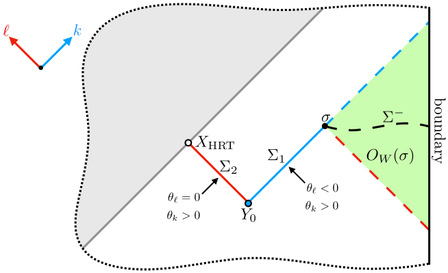
Figure 2: Portion of a Penrose diagram illustrating our construction of an HRT surface realizing the outer entropy. Holding the outer wedge (green) fixed, we choose data on $N_{-k}(\sigma)$ (blue line) as described in text until we reach a surface $Y_{0}$ (blue dot) on which $\theta_{\ell}=0$. We choose a gauge such that $Y_{0}$ is marginally antitrapped, $Y_{0}=Y_{\rm MA}$. Again choosing data as described in Sec. 3.2, we follow the light sheet $N_{+\ell}(Y_{0})$ (red line) until we reach a surface $X_{0}$ on which $\theta_{k}=0$, provided $\partial_{\ell}\theta_{k}<0$ on $Y_{\rm MA}$, which we assume. As discussed in the text, the existence of $X_{0}$ guarantees the existence of an HRT surface $X_{\rm HRT}$ (white dot) on $N_{+k}(Y_{0})$. The entire spacetime is completed (gray shading) by CPT-reflecting the initial value data on $\Sigma^{-}\cup\Sigma_{1}\cup\Sigma_{2}$.

To find the expression for $A[X_{\rm HRT}]$, we still need to construct the appropriate surface $Y_{0}$ by solving the constraint equations on $N_{-k}(\sigma)$. We now turn to this problem.

3.3 Solution to the constraint equations

Let us solve the constraint equations (13), given our choice (12) of initial data. By inverting the Raychaudhuri equation, we can solve $\theta_{k}(\nu)$ at $x^{i}$ as a function of $\theta_{k}[\sigma]$ at the same $x^{i}$:

$$\theta_{k}(\nu)=\left[\frac{1}{\theta_{k}[\sigma]}+\frac{\nu}{D-2}\right]^{-1}.$$ (15)

We will leave the $x^{i}$ arguments implicit everywhere. We find it convenient to introduce a new variable $\xi$, a function of $\nu$ and $x^{i}$, to parameterize distance along $N_{k}(\sigma)$, defined by

$$\xi(\nu)=\frac{\theta_{k}(\nu)}{\theta_{k}[\sigma]}=\left[1+\frac{\nu\theta_{k}[\sigma]}{D-2}\right]^{-1}.$$ (16)

We note that $\xi=1$ corresponds to $\sigma$ and $\xi>1$ corresponds to slices of $N_{-k}(\sigma)$. In terms of $\xi$, the derivative operator is

$$\partial_{k}=\frac{\partial\xi}{\partial\nu}\partial_{\xi}=\frac{\partial_{k}\theta_{k}}{\theta_{k}[\sigma]}\partial_{\xi}=-\frac{1}{D-2}\xi^{2}\theta_{k}[\sigma]\partial_{\xi}.$$ (17)

We can write $\theta_{k}$ in the Raychaudhuri equation in Eq. (13) as $\xi\theta_{k}[\sigma]$ and, since

$${\cal D}_{i}\xi=-\frac{\frac{\nu}{D-2}}{\left[1+\frac{\nu\theta_{k}[\sigma]}{D-2}\right]^{2}}{\cal D}_{i}\theta_{k}[\sigma]=\left(\xi^{2}-\xi\right){\cal D}_{i}\log\theta_{k}[\sigma],$$ (18)

we have the nice expression

$${\cal D}_{i}\theta_{k}(\xi)=\xi{\cal D}_{i}\theta_{k}[\sigma]+\theta_{k}[\sigma]{\cal D}_{i}\xi=\xi^{2}{\cal D}_{i}\theta_{k}[\sigma].$$ (19)

Hence, the DNS equation in Eq. (13) becomes

$$\xi\partial_{\xi}\omega_{i}=(D-2)\omega_{i}-(D-3)\xi{\cal D}_{i}\log\theta_{k}[\sigma],$$ (20)

which has solution

$$\omega_{i}(\xi)=\omega_{i}[\sigma]\xi^{D-2}+\left(\xi-\xi^{D-2}\right){\cal D}_{i}\log\theta_{k}[\sigma].$$ (21)

By Eq. (15) we have satisfied the Raychaudhuri equation in Eq. (13), and by Eq. (21) we have satisfied the DNS equation. It remains to compute the terms in the cross-focusing equation to solve for $\theta_{\ell}$ as a function of $\xi$. Let us consider each term in turn.

Since $\partial_{k}g_{ij}=\frac{2}{D-2}\theta_{k}g_{ij}$, we have $\partial_{k}\log{\cal R}=-\frac{2}{D-2}\theta_{k}$, or equivalently, $\xi\partial_{\xi}\log{\cal R}=2$, so

$${\cal R}(\xi)=\xi^{2}{\cal R}[\sigma].$$ (22)

Similarly, $\partial_{k}g^{ij}=-\frac{2}{D-2}\theta_{k}g^{ij}$ as shown in footnote 4, so $\xi\partial_{\xi}g^{ij}=2g^{ij}$, which has solution $g^{ij}(\xi)=\xi^{2}g^{ij}[\sigma]$. (Here, $i$ and $j$ are transverse indices, so we could write $q_{ij}$ everywhere for $g_{ij}$ in this statement.) Since $\omega^{i}(\xi)=g^{ij}(\xi)\omega_{j}(\xi)$, we therefore obtain

$$\omega^{2}(\xi) =\xi^{2}g^{ij}[\sigma]\omega_{i}(\xi)\omega_{j}(\xi)$$ (23)

$$=\xi^{2(D-1)}\omega^{2}[\sigma]+2\left(\xi^{3}-\xi^{D}\right)\xi^{D-2}\omega^{i}[\sigma]{\cal D}_{i}\log\theta_{k}[\sigma]$$

$$\qquad+\left(\xi^{2}-\xi^{D-1}\right)^{2}{\cal D}^{i}\log\theta_{k}[\sigma]{\cal D}_{i}\log\theta_{k}[\sigma].$$

We can similarly compute ${\cal D}\cdot\omega$ as a function of $\xi$. Recalling the expression in Eq. (18) for ${\cal D}_{i}\xi$ and the fact that $q^{ab}(\xi)=\xi^{2}q^{ab}[\sigma]$, we have

$${\cal D}\cdot\omega(\xi) =\left(\xi^{2}-\xi\right)\left[\xi^{2}-(D-2)\xi^{D-1}\right]\left({\cal D}_{i}\log\theta_{k}[\sigma]\right)^{2}$$ (24)

$$\qquad+(D-2)\left(\xi^{D+1}-\xi^{D}\right)\omega^{i}[\sigma]{\cal D}_{i}\log\theta_{k}[\sigma]$$

$$\qquad+\left(\xi^{3}-\xi^{D}\right)\Box\log\theta_{k}[\sigma]+\xi^{D}{\cal D}\cdot\omega[\sigma],$$

where $\Box={\cal D}\cdot{\cal D}$.

Let us define $q(\nu,x^{i})$ such that

$$\theta_{\ell}=\theta_{\ell}[\sigma]\frac{q}{\xi}.$$ (25)

Then

$$\partial_{k}\theta_{\ell}=-\frac{1}{D-2}\xi^{2}\theta_{k}[\sigma]\partial_{\xi}\theta_{\ell}=-\frac{1}{D-2}\theta_{k}[\sigma]\theta_{\ell}[\sigma]\left(\xi\partial_{\xi}q-q\right).$$ (26)

The right-hand side of the cross-focusing equation becomes

$$-\frac{1}{2}{\cal R}-\theta_{k}\theta_{\ell}+\omega^{2}+{\cal D}\cdot\omega+\Lambda$$ (27)

$$\qquad=-\frac{1}{2}\xi^{2}{\cal R}[\sigma]-\theta_{k}[\sigma]\theta_{\ell}[\sigma]q+\Lambda$$

$$\qquad\;\;\;\;+\left[\xi^{2D-2}-D\xi^{D+1}+(D-2)\xi^{D}+2\xi^{4}-\xi^{3}\right]\left({\cal D}_{i}\log\theta_{k}[\sigma]\right)^{2}$$

$$\qquad\;\;\;\;-\left[2\xi^{2D-2}-D\xi^{D+1}+(D-2)\xi^{D}\right]\omega^{i}[\sigma]{\cal D}_{i}\log\theta_{k}[\sigma]$$

$$\qquad\;\;\;\;+\left(\xi^{3}-\xi^{D}\right)\Box\log\theta_{k}[\sigma]+\xi^{D}{\cal D}\cdot\omega[\sigma]+\xi^{2D-2}\omega^{2}[\sigma],$$

so we have

$$-\frac{1}{D-2}\xi\partial_{\xi}q+\frac{D-1}{D-2}q =-\frac{1}{2}\xi^{2}\frac{{\cal R}[\sigma]}{\theta_{k}[\sigma]\theta_{\ell}[\sigma]}+\frac{\Lambda}{\theta_{k}[\sigma]\theta_{\ell}[\sigma]}$$ (28)

$$\qquad+\left[\xi^{2D-2}-D\xi^{D+1}+(D-2)\xi^{D}+2\xi^{4}-\xi^{3}\right]\frac{\left({\cal D}_{i}\log\theta_{k}[\sigma]\right)^{2}}{\theta_{k}[\sigma]\theta_{\ell}[\sigma]}$$

$$\qquad-\left[2\xi^{2D-2}-D\xi^{D+1}+(D-2)\xi^{D}\right]\frac{\omega^{i}[\sigma]{\cal D}_{i}\log\theta_{k}[\sigma]}{\theta_{k}[\sigma]\theta_{\ell}[\sigma]}$$

$$\qquad+\left(\xi^{3}-\xi^{D}\right)\frac{\Box\log\theta_{k}[\sigma]}{\theta_{k}[\sigma]\theta_{\ell}[\sigma]}+\xi^{D}\frac{{\cal D}\cdot\omega[\sigma]}{\theta_{k}[\sigma]\theta_{\ell}[\sigma]}+\xi^{2D-2}\frac{\omega^{2}[\sigma]}{\theta_{k}[\sigma]\theta_{\ell}[\sigma]}.$$

We want to choose a gauge in which the zero $\xi_{0}(x^{i})$ of $q$ (for $q$ solving Eq. (28)) occurs at a uniform affine parameter, $\nu=\nu_{0}$ for all $x^{i}$ (i.e., $1/\xi_{0}(x^{i})=1+\frac{\nu_{0}\theta_{k}[\sigma]}{D-2}$, where the $x^{i}$-dependence in $\xi_{0}$ tracks the $x^{i}$-dependence in $\theta_{k}[\sigma]$), thus making $Y_{0}$ a marginally-antitrapped surface, $Y_{0}=Y_{\rm MA}$. That is, computing the zero $\xi_{0}(x^{i})$ along each null generator, indexed by $x^{i}$, we need

$${\cal D}_{i}\xi_{0}=\left(\xi_{0}^{2}-\xi_{0}\right){\cal D}_{i}\log\theta_{k}[\sigma]$$ (29)

for all $x^{i}$, as in Eq. (18). Let us first solve for $q$ in Eq. (28) without making any a priori choice of the normalization of $k$ and then subsequently use gauge freedom to guarantee Eq. (29) so that $\nu_{0}$ is independent of $x^{i}$. Let us define the right-hand side of Eq. (28) to be a function $f(\xi,x^{i})$, where the $x^{i}$-dependence enters only through the dependence of $\theta_{k}[\sigma]$, $\theta_{\ell}[\sigma]$, ${\cal R}[\sigma]$, and $\omega_{a}[\sigma]$ on their transverse position on $\sigma$. The differential equation for $q$ can be written as

$$f=-\frac{1}{D-2}\xi^{D}\partial_{\xi}\left(\frac{q}{\xi^{D-1}}\right),$$ (30)

which has solution

$$q(\xi)=-(D-2)\xi^{D-1}\int{\rm d}\xi\frac{f}{\xi^{D}},$$ (31)

where the integration constant is set by requiring $q=1$ at $\xi=1$.

Explicitly, defining $\psi_{i}[\sigma]=\omega_{i}[\sigma]-{\cal D}_{i}\log\theta_{k}[\sigma]$, we have

$$q(\xi) =\left(1-\lambda-\rho-\epsilon_{1}-\epsilon_{2}-\epsilon_{3}-\epsilon_{4}-\epsilon_{5}\right)\xi^{D-1}$$ (32)

$$\qquad+\lambda+\rho\xi^{2}+\epsilon_{1}\xi^{3}+\epsilon_{2}\xi^{4}+\epsilon_{3}\xi^{D}+\epsilon_{4}\xi^{D+1}+\epsilon_{5}\xi^{2D-2},$$

where

$$\lambda =\frac{D-2}{D-1}\frac{\Lambda}{\theta_{k}[\sigma]\theta_{\ell}[\sigma]}$$ (33)

$$\rho =-\frac{1}{2}\frac{D-2}{D-3}\frac{{\cal R}[\sigma]}{\theta_{k}[\sigma]\theta_{\ell}[\sigma]}$$

$$\epsilon_{1} =\frac{D-2}{D-4}\frac{\Box\log\theta_{k}[\sigma]-({\cal D}_{i}\log\theta_{k}[\sigma])^{2}}{\theta_{k}[\sigma]\theta_{\ell}[\sigma]}$$

$$\epsilon_{2} =2\frac{D-2}{D-5}\frac{({\cal D}_{i}\log\theta_{k}[\sigma])^{2}}{\theta_{k}[\sigma]\theta_{\ell}[\sigma]}$$

$$\epsilon_{3} =-(D-2)\frac{{\cal D}\cdot\psi[\sigma]-(D-2)\psi^{i}[\sigma]{\cal D}_{i}\log\theta_{k}[\sigma]}{\theta_{k}[\sigma]\theta_{\ell}[\sigma]}$$

$$\epsilon_{4} =-\frac{D(D-2)}{2}\frac{\psi^{i}[\sigma]{\cal D}_{i}\log\theta_{k}[\sigma]}{\theta_{k}[\sigma]\theta_{\ell}[\sigma]}$$

$$\epsilon_{5} =-\frac{D-2}{D-1}\frac{\psi^{2}[\sigma]}{\theta_{k}[\sigma]\theta_{\ell}[\sigma]}.$$

Note that $\epsilon_{1,2,3,4,5}$ vanish for spherically-symmetric geometries in an appropriate gauge, while $\epsilon_{3,4,5}$ vanish if $\psi_{i}[\sigma]=0$. In Eq. (33), we have taken $D\geq 6$. For the special cases of $D=3,4,5$, we can derive the analogues of Eq. (32) and Eq. (33), which we now compute.

3.3.1 $D=3$

For $D=3$, $\cal R$ vanishes, and the analogue of the right-hand side of Eq. (28) is

$$f(\xi,x^{i})=\frac{\Lambda}{\theta_{k}[\sigma]\theta_{\ell}[\sigma]}+\xi^{3}\frac{{\cal D}\cdot\omega[\sigma]-\omega^{i}[\sigma]{\cal D}_{i}\log\theta_{k}[\sigma]}{\theta_{k}[\sigma]\theta_{\ell}[\sigma]}+\xi^{4}\frac{\omega^{i}[\sigma]{\cal D}_{i}\log\theta_{k}[\sigma]+\omega^{2}[\sigma]}{\theta_{k}[\sigma]\theta_{\ell}[\sigma]},$$ (34)

so

$$q(\xi)=\left(1-\lambda-\chi-\tau\right)\xi^{2}+\lambda+\chi\xi^{3}+\tau\xi^{4},$$ (35)

where

$$\lambda =\frac{\Lambda}{2\theta_{k}[\sigma]\theta_{\ell}[\sigma]}$$ (36)

$$\chi =-\frac{{\cal D}\cdot\omega[\sigma]-\omega^{i}[\sigma]{\cal D}_{i}\log\theta_{k}[\sigma]}{\theta_{k}[\sigma]\theta_{\ell}[\sigma]}$$

$$\tau =-\frac{\omega^{i}[\sigma]{\cal D}_{i}\log\theta_{k}[\sigma]+\omega^{2}[\sigma]}{2\theta_{k}[\sigma]\theta_{\ell}[\sigma]}.$$

3.3.2 $D=4$

For $D=4$, the analogue of the right-hand side of Eq. (28) is

$$f(\xi,x^{i}) =-\frac{1}{2}\xi^{2}\frac{{\cal R}[\sigma]}{\theta_{k}[\sigma]\theta_{\ell}[\sigma]}+\frac{\Lambda}{\theta_{k}[\sigma]\theta_{\ell}[\sigma]}$$ (37)

$$\qquad+\left(\xi^{6}-4\xi^{5}+4\xi^{4}-\xi^{3}\right)\frac{\left({\cal D}_{i}\log\theta_{k}[\sigma]\right)^{2}}{\theta_{k}[\sigma]\theta_{\ell}[\sigma]}$$

$$\qquad-2\left(\xi^{6}-2\xi^{5}+\xi^{4}\right)\frac{\omega^{i}[\sigma]{\cal D}_{i}\log\theta_{k}[\sigma]}{\theta_{k}[\sigma]\theta_{\ell}[\sigma]}$$

$$\qquad+\left(\xi^{3}-\xi^{4}\right)\frac{\Box\log\theta_{k}[\sigma]}{\theta_{k}[\sigma]\theta_{\ell}[\sigma]}+\xi^{4}\frac{{\cal D}\cdot\omega[\sigma]}{\theta_{k}[\sigma]\theta_{\ell}[\sigma]}+\xi^{6}\frac{\omega^{2}[\sigma]}{\theta_{k}[\sigma]\theta_{\ell}[\sigma]},$$

so

$$q(\xi)=(1-\lambda-\rho-\epsilon_{23}-\epsilon_{4}-\epsilon_{5})\xi^{3}+\lambda+\rho\xi^{2}+\phi_{1}\xi^{3}\log\xi+\epsilon_{23}\xi^{4}+\epsilon_{4}\xi^{5}+\epsilon_{5}\xi^{6},$$ (38)

where

$$\lambda =\frac{2\Lambda}{3\theta_{k}[\sigma]\theta_{\ell}[\sigma]}$$ (39)

$$\rho =-\frac{{\cal R}[\sigma]}{\theta_{k}[\sigma]\theta_{\ell}[\sigma]}$$

$$\phi_{1} =-2\frac{\Box\log\theta_{k}[\sigma]-({\cal D}_{i}\log\theta_{k}[\sigma])^{2}}{\theta_{k}[\sigma]\theta_{\ell}[\sigma]}$$

$$\epsilon_{23} =-2\frac{4({\cal D}_{i}\log\theta_{k}[\sigma])^{2}+{\cal D}\cdot\psi[\sigma]-2\omega^{i}[\sigma]{\cal D}_{i}\log\theta_{k}[\sigma]}{\theta_{k}[\sigma]\theta_{\ell}[\sigma]}$$

$$\epsilon_{4} =-\frac{4\psi^{i}[\sigma]{\cal D}_{i}\log\theta_{k}[\sigma]}{\theta_{k}[\sigma]\theta_{\ell}[\sigma]}$$

$$\epsilon_{5} =-\frac{2\psi^{2}[\sigma]}{3\theta_{k}[\sigma]\theta_{\ell}[\sigma]}.$$

Note that $\phi_{1}=-\lim_{D\rightarrow 4}(D-4)\epsilon_{1}$, where $\epsilon_{1}$ is defined in Eq. (33), and that $\epsilon_{23}=\epsilon_{2}+\epsilon_{3}$ evaluated at $D=4$.

3.3.3 $D=5$

Finally, let us consider the special case of $D=5$. The analogue of the right-hand side of Eq. (28) is

$$f(\xi,x^{i}) =-\frac{1}{2}\xi^{2}\frac{{\cal R}[\sigma]}{\theta_{k}[\sigma]\theta_{\ell}[\sigma]}+\frac{\Lambda}{\theta_{k}[\sigma]\theta_{\ell}[\sigma]}$$ (40)

$$\qquad+\left(\xi^{8}-5\xi^{6}+3\xi^{5}+2\xi^{4}-\xi^{3}\right)\frac{\left({\cal D}_{i}\log\theta_{k}[\sigma]\right)^{2}}{\theta_{k}[\sigma]\theta_{\ell}[\sigma]}$$

$$\qquad-\left(2\xi^{8}-5\xi^{6}+3\xi^{5}\right)\frac{\omega^{i}[\sigma]{\cal D}_{i}\log\theta_{k}[\sigma]}{\theta_{k}[\sigma]\theta_{\ell}[\sigma]}$$

$$\qquad+\left(\xi^{3}-\xi^{5}\right)\frac{\Box\log\theta_{k}[\sigma]}{\theta_{k}[\sigma]\theta_{\ell}[\sigma]}+\xi^{5}\frac{{\cal D}\cdot\omega[\sigma]}{\theta_{k}[\sigma]\theta_{\ell}[\sigma]}+\xi^{8}\frac{\omega^{2}[\sigma]}{\theta_{k}[\sigma]\theta_{\ell}[\sigma]},$$

so

$$q(\xi)=\left(1-\lambda-\rho-\epsilon_{1}-\epsilon_{3}-\epsilon_{4}-\epsilon_{5}\right)\xi^{4}+\lambda+\rho\xi^{2}+\epsilon_{1}\xi^{3}+\phi_{2}\xi^{4}\log\xi+\epsilon_{3}\xi^{5}+\epsilon_{4}\xi^{6}+\epsilon_{5}\xi^{8},$$ (41)

where

$$\lambda =\frac{3\Lambda}{4\theta_{k}[\sigma]\theta_{\ell}[\sigma]}$$ (42)

$$\rho =-\frac{3{\cal R}[\sigma]}{4\theta_{k}[\sigma]\theta_{\ell}[\sigma]}$$

$$\epsilon_{1} =3\frac{\Box\log\theta_{k}[\sigma]-({\cal D}_{i}\log\theta_{k}[\sigma])^{2}}{\theta_{k}[\sigma]\theta_{\ell}[\sigma]}$$

$$\phi_{2} =-6\frac{({\cal D}_{i}\log\theta_{k}[\sigma])^{2}}{\theta_{k}[\sigma]\theta_{\ell}[\sigma]}$$

$$\epsilon_{3} =-3\frac{{\cal D}\cdot\psi[\sigma]-3\psi^{i}[\sigma]{\cal D}_{i}\log\theta_{k}[\sigma]}{\theta_{k}[\sigma]\theta_{\ell}[\sigma]}$$

$$\epsilon_{4} =-\frac{15\psi^{i}[\sigma]{\cal D}_{i}\log\theta_{k}[\sigma]}{2\theta_{k}[\sigma]\theta_{\ell}[\sigma]}$$

$$\epsilon_{5} =-\frac{3\psi^{2}[\sigma]}{4\theta_{k}[\sigma]\theta_{\ell}[\sigma]}.$$

Note that $\phi_{2}=-\lim_{D\rightarrow 5}(D-5)\epsilon_{2}$, where $\epsilon_{2}$ is given in Eq. (33).

3.4 Gauge fixing

The surface $Y_{0}$ occurs at the first zero $\xi_{0}$ of $q$. To require that the affine parameter $\nu=\nu_{0}$ at which this zero occurs to the same along every generator of $N_{-k}(\sigma)$, which would make $Y_{0}$ a bona fide marginally antitrapped surface as required, we need Eq. (29) to be satisfied. Suppose we first compute $\xi_{0}$ as a function of $x^{i}$ and find that it does not satisfy Eq. (29), which would mean that $q$ does not vanish at constant affine parameter. We can subsequently gauge transform the normalization of $k$ to enforce Eq. (29). Let us define a rescaling of the vectors on $\sigma$ of the form

$$k^{a} \rightarrow e^{\Gamma}k^{a}$$ (43)

$$\ell^{a} \rightarrow e^{-\Gamma}\ell^{a}.$$

Then the affine parameter transforms as $\nu\rightarrow e^{-\Gamma}\nu$. Our $\xi$ parameter is invariant under this gauge transformation, $\xi\rightarrow\xi$. However, the value of $\xi$ at which $q$ vanishes can change, since our various curvature quantities transform as

$$\theta_{k}[\sigma] \rightarrow e^{\Gamma}\theta_{k}[\sigma]$$ (44)

$$\theta_{\ell}[\sigma] \rightarrow e^{-\Gamma}\theta_{\ell}[\sigma]$$

$$\omega_{i}[\sigma] \rightarrow\omega_{i}[\sigma]+{\cal D}_{i}\Gamma$$

$${\cal R}[\sigma] \rightarrow{\cal R}[\sigma]$$

$$\psi_{i}[\sigma] \rightarrow\psi_{i}[\sigma].$$

Once we gauge fix so that Eq. (29) is satisfied, we are guaranteed that $Y_{0}$, the surface on which $\theta_{\ell}=0$, is indeed marginally antitrapped.

We can then construct an HRT surface by flowing along $N_{+\ell}(Y_{0})$ as described in Sec. 3.2. For this construction to work, we need $\partial_{\ell}\theta_{k}<0$ on $Y_{0}$. The cross-focusing equation gives

$$\partial_{\ell}\theta_{k}=-\frac{1}{2}{\cal R}-\theta_{\ell}\theta_{k}+\omega^{2}-{\cal D}\cdot\omega+8\pi G\,T_{k\ell}+\Lambda=\partial_{k}\theta_{\ell}-2{\cal D}\cdot\omega.$$ (45)

At $\xi_{0}$, we have $\partial_{k}\theta_{\ell}=-\frac{1}{D-2}\theta_{k}[\sigma]\theta_{\ell}[\sigma]\xi\partial_{\xi}q=\theta_{k}[\sigma]\theta_{\ell}[\sigma]f$ by Eqs. (26) and (30). Since $\xi_{0}$ by definition is the first zero of $q$ for $\xi>1$ and $q(\xi=1)=1$, we have $\partial_{\xi}q\leq 0$ at $\xi_{0}$, so it follows that $\partial_{k}\theta_{\ell}\leq 0$ at $\xi_{0}$. By Eq. (45), the requirement that $\partial_{\ell}\theta_{k}<0$ is a slightly different condition. Provided this condition is satisfied, the area of the HRT surface is calculated from $\xi_{0}$:

$$A[X_{{\rm HRT}}]=\oint_{\sigma}\frac{\epsilon}{[\xi_{0}(x^{i})]^{D-2}}.$$ (46)

where the integral is computed with the standard area $(D-2)$-form $\epsilon$ defined on $\sigma$ (so the area of $\sigma$ is just $A[\sigma]=\oint_{\sigma}\epsilon$).

There are two conditions that must be satisfied for our construction of this HRT surface to work:

1. There must exist a gauge transformation (44) such that a solution $\xi_{0}$ of $q(\xi_{0})=0$ exists everywhere on $\sigma$ for $\xi_{0}(x^{i})$ satisfying Eq. (29).

2. We must have $\partial_{\ell}\theta_{k}[Y_{0}]<0$.

Condition 1 guarantees that we reach a $\theta_{\ell}=0$ surface before $\theta_{k}$ diverges. If, in a given gauge, $q(\xi)=0$ cannot be satisfied along some null generator, it means that the geodesic in question hits a caustic before we reach a surface where $\theta_{\ell}$ vanishes. That is, one can show that condition 1 guarantees that we have a one-to-one mapping along null generators from $\sigma$ to $Y_{0}$. Moreover, the requirement in condition 1 that $\xi_{0}$ satisfy Eq. (29) is necessary to guarantee that the affine parameter corresponding to the zero of $q$ is independent of $x^{i}$, so that $Y_{0}$ is a marginally-antitrapped surface as discussed in Sec. 3.2. Finally, condition 2 is necessary to guarantee that $Y_{0}$ is a minimar surface in the sense of LABEL:Engelhardt:2018kcs, so that we actually reach an HRT surface by flowing along $N_{+\ell}(Y_{0})$. If one can freely solve the algebraic equation for $q(\xi)=0$, then conditions 1 and 2 can all be checked using the data on $\sigma$.

These conditions act as vetoes for surfaces $\sigma$: if $\sigma$ fails any of these conditions, our construction does not apply, and one must choose a different surface. For a surface on which $N_{-k}(\sigma)$ unavoidably encounters caustics before reaching the $\theta_{\ell}=0$ surface (see Fig. 3), we could imagine relaxing condition 1 and instead merely find some maximal subset of the generators on $\sigma$ for which conditions 1 and 2 can be satisfied. That is, if any geodesic cannot solve $q(\xi)=0$, we can drop that geodesic, since it must reach a caustic before going through $Y_{0}$. However, in this case, we do not have the guarantee discussed in footnote 8, and we cannot rule out the possibility that some geodesics go through nonlocal intersections before encountering $Y_{0}$. For such surfaces, our algorithm would therefore give an upper bound on the outer entropy (modulo the conjecture that the choice in Eq. (12) is optimal).

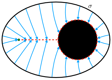
Figure 3: Illustration of a choice of a codimension-two surface $\sigma$ (black line) that does not satisfy our veto condition 1. The light sheet in the $-k$ direction (blue arrows) unavoidably encounters a caustic (green dot) along some generator before reaching the marginally-antitrapped surface $Y_{\rm MA}$ (black circle). Thus, the surface (red dashed line) spanned by a slice of $N_{-k}(\sigma)$, defined such that each generator either has $\theta_{\ell}=0$ or encounters a nonlocal intersection or caustic, has area larger than the HRT surface.

More generally, one can compute the outer entropy for an arbitrary surface $\sigma$ failing condition 1 without using our explicit algorithm, although such a computation would be challenging in practice. For an arbitrary surface $\sigma$, consider the extension of $O_{W}(\sigma)$ to a spacetime ${\cal M}$ for which the HRT surface interior to $\sigma$ is maximized. Then rather than using our explicit algorithm, one can define $Y_{0}$ to be the intersection of $N_{-\tilde{\ell}}(X_{\rm HRT})$ with $N_{-k}(\sigma)$, where $\tilde{\ell}$ is defined to be the ingoing null geodesic congruence orthogonal to $X_{\rm HRT}$, with zero shear. If, as we have assumed, choosing $T_{ab}$ to vanish in $\overline{D}(\Sigma^{+}(\sigma))$ results in the optimal HRT surface, then the surface $Y_{0}$ exists in the spacetime, since the light sheet $N_{-\tilde{\ell}}(X_{\rm HRT})$ never ends and always has cross section with area equal to $A[X_{\rm HRT}]$. If conditions 1 and 2 are satisfied, then there is a one-to-one correspondence between $Y_{0}$ and $\sigma$ induced by the geodesic congruence from $\sigma$ along the $-k$ direction. If condition 1 fails, then one must relate $A[\sigma]$ and $A[X_{\rm HRT}]$ in the full spacetime by keeping track of which geodesics exit $N_{-k}(\sigma)$ between $\sigma$ and $Y_{0}$. Even in this case, however, condition 2 is still needed, to guarantee that $\theta_{k}$ is positive on $Y_{0}$ so that $\sigma$ is a normal surface.

4 Optimization

We now argue that our choices in Eq. (12) indeed give the optimal HRT surface, so that the outer entropy is given simply by Eq. (46),

$$S^{({\rm outer})}[\sigma]=\frac{1}{4G\hbar}\oint_{\sigma}\frac{\epsilon}{[\xi_{0}(x^{i})]^{D-2}}.$$ (47)

This is one of the main results of this work: an algorithm for computing the outer entropy (i.e., the area of the maximal HRT surface) for general codimension-two surfaces in general spacetimes. We will give plausible physical arguments for why the choice (12) should maximize the area of the HRT surface and hence conjecture that Eq. (47) holds, leaving a formal mathematical proof to future work. Throughout, we assume the NEC, along with the version of the dominant energy condition that ignores the cosmological constant (dubbed the $\Lambda$DEC in LABEL:Nomura:2018aus), which requires that $-T^{a}_{\;\;b}t^{b}$ be a future-directed, causal vector for all future-directed, causal $t^{a}$, so that the energy-momentum flow (excepting the cosmological constant) is causal in any reference frame. In particular, the $\Lambda$DEC implies that $T_{k\ell}\geq 0$, just as the NEC implies that $T_{kk}$ and $T_{\ell\ell}$ are nonnegative.

In the spherically-symmetric case, where the twist and shear vanish identically, the optimality of the choice $T_{kk}=T_{k\ell}=0$, given the NEC and $\Lambda$DEC, was established in detail in LABEL:Nomura:2018aus. Here, we simply mention that the reason for this can be inferred from the constraint equations (9): nonzero $T_{kk}$ would cause $\theta_{k}$ to grow more positive as we move toward the past along $N_{-k}(\sigma)$, and this would in turn increase $\nabla_{k}\theta_{\ell}$, which we want to engineer to be as negative as possible in order to reach the surface $X$ while incurring the least change in area from $\sigma$.

An essentially identical motivates us to take $T_{kk}$ and $T_{k\ell}$ to vanish in the general, nonspherical case. Similarly, nonzero shear contributes to the Raychaudhuri equation in such a way as to accelerate the growth of $\theta_{k}$ along $N_{-k}(\sigma)$, counter to what we want for the construction, so we set $\varsigma_{k}$ to zero. As for the twist $\omega_{a}$, the ${\cal D}\cdot\omega$ term in the cross-focusing equation can contribute with either sign, but since its integral over any slice of $N_{-k}(\sigma)$ vanishes, it has no average effect on $\nabla_{k}\theta_{\ell}$ (though it can affect the global solution for $\xi_{0}$ due to its variation over $\sigma$). On the other hand, the $\omega^{2}$ term has definite sign, making $\theta_{\ell}$ approach zero more slowly as we move along $N_{-k}(\sigma)$ and thereby decreasing $A[Y_{0}]$, which we do not want. Once we have chosen $T_{ak}=\varsigma_{k}=0$, the evolution of $\omega_{a}$ from its value on $\sigma$ is fixed by the DNS equation. Therefore, to combat the deleterious effect of $\omega_{a}$, we could only imagine shutting off $\omega_{a}$ immediately to the past of $\sigma$ along $N_{-k}(\sigma)$ via a shock wave of nonzero $T_{ak}$ that cancels off $\omega_{a}[\sigma]$ precisely. However, as we will see below, this operation comes at a cost.

Let us define $v_{a}=-T_{ak}$, which the $\Lambda$DEC implies must be causal and future-directed, so $v^{2}\leq 0$. Since $g^{k\ell}=-1$, this implies $v_{i}v^{i}\leq 2v_{k}v_{\ell}$. Thus,

$$g^{ij}T_{ik}T_{jk}\leq 2T_{kk}T_{k\ell}.$$ (48)

In particular, a consequence of the $\Lambda$DEC is that setting $T_{kk}=T_{k\ell}=0$ implies $T_{ak}=0$ (and similarly, setting $T_{\ell\ell}=0$ and $T_{k\ell}=0$ implies $T_{a\ell}=0$).

Suppose that $8\pi G\,T_{ik}(\nu)=\delta(\nu)\omega_{i}[\sigma]$, corresponding to a shell of rotating matter. By the DNS equation in Eq. (9), the effect of this nonzero $T_{ik}$ is to zero out $\omega^{2}$ to the past of $\sigma$ along $N_{-k}(\sigma)$. We saturate the $\Lambda$DEC by taking $8\pi G\,T_{kk}=\frac{x}{\sqrt{2}}\sqrt{\omega^{2}[\sigma]}\delta(\nu)$ and $8\pi G\,T_{k\ell}=\frac{1}{x\sqrt{2}}\sqrt{\omega^{2}[\sigma]}\delta(\nu)$ for some parameter $x$. By the NEC, $x\geq 0$. What does this shell of nonzero $T_{kk}$ and $T_{k\ell}$ do to $\theta_{k}$ and $\theta_{\ell}$? It shifts them from their values on $\sigma$ to new values immediately to the past along $N_{-k}(\sigma)$. That is, with $\nu=0$ corresponding to $\sigma$, we have $\theta_{k}(\nu\rightarrow 0^{-})=\theta_{k}[\sigma]+\Delta\theta_{k}$ and $\theta_{\ell}(\nu\rightarrow 0^{-})=\theta_{\ell}[\sigma]+\Delta\theta_{\ell}$, where

$$\Delta\theta_{k} =8\pi G\,\int_{-\epsilon}^{\epsilon}{\rm d}\nu\,T_{kk}(\nu)$$ (49)

$$\Delta\theta_{\ell} =-8\pi G\,\int_{-\epsilon}^{\epsilon}{\rm d}\nu\,T_{k\ell}(\nu).$$

Moving further along $N_{-k}(\sigma)$, to the past of these shifts, the solution proceeds in the same way as before, with $T_{kk}$ and $T_{k\ell}$ vanishing. Hence, the cost of zeroing out $\omega^{2}$ is to shift $\theta_{k}$ and $\theta_{\ell}$. Note that both shifts have signs that will decrease the area of $Y_{0}$, counter to our desired outcome.

A concrete example is illuminating. Let us take an axisymmetric spacetime in $D=3$, with $\sigma$ a circle centered on the origin, so that $\omega_{a}[\sigma]$ is a constant covector pointing in the angular direction and we choose a gauge in which $\theta_{k}$ and $\theta_{\ell}$ are constant over $\sigma$. In this case, the $\chi$ term in Eq. (36) vanishes. With our choice of nonzero $T_{ik}$ to cancel $\omega_{i}$, the $\tau$ term in Eq. (36) would also drop out, making $q=(1-\lambda^{\prime})\xi^{2}+\lambda^{\prime}$, so the zero $\xi_{0}^{\prime}$ is given by

$$\xi_{0}^{\prime}=\left(1-\frac{1}{\lambda^{\prime}}\right)^{-1/2},$$ (50)

where $\lambda^{\prime}$ is $\lambda$ but with $\theta_{k}$ and $\theta_{\ell}$ shifted:

$$\lambda^{\prime}=\frac{\Lambda}{2\left(\theta_{k}[\sigma]+\Delta\theta_{k}\right)\left(\theta_{\ell}[\sigma]+\Delta\theta_{\ell}\right)}=\frac{\Lambda}{2\left[\theta_{k}[\sigma]\theta_{\ell}[\sigma]-\frac{\omega^{2}[\sigma]}{2}+\sqrt{\frac{\omega^{2}[\sigma]}{2}}\left(x\theta_{\ell}[\sigma]-\frac{1}{x}\theta_{k}[\sigma]\right)\right]}.$$ (51)

To minimize $\xi_{0}^{\prime}$, we want $\lambda^{\prime}$ to be maximized, which occurs when $x=\sqrt{-\theta_{k}[\sigma]/\theta_{\ell}[\sigma]}$, so

$$\lambda^{\prime}=-\frac{\Lambda}{2\left(\sqrt{-\theta_{\ell}[\sigma]\theta_{k}[\sigma]}+\sqrt{\frac{\omega^{2}[\sigma]}{2}}\right)^{2}}.$$ (52)

In contrast, if we instead take the construction of Sec. 3 with the choice of data given in Eq. (12), then we find the zero of $q(\xi)=(1-\lambda-\tau)\xi^{2}+\lambda+\tau\xi^{4}$ (recalling that we are still taking $\chi=0$ by axisymmetry) at

$$\xi_{0}=\left[\frac{-(1-\lambda-\tau)\pm\sqrt{\left(1-\lambda-\tau\right)^{2}-4\lambda\tau}}{2\tau}\right]^{1/2},$$ (53)

where $\lambda=\Lambda/2\theta_{k}[\sigma]\theta_{\ell}[\sigma]$ and $\tau=-\omega^{2}[\sigma]/2\theta_{k}[\sigma]\theta_{\ell}[\sigma]$ from Eq. (36). We choose the $-$ branch of the $\pm$ in Eq. (53) since we are interested in the smallest solution for $\xi\geq 1$ (i.e., the first time $N_{-k}(\sigma)$ goes through a $\theta_{\ell}=0$ surface). Such a solution with $\xi_{0}\geq 1$ exists if and only if

$$\lambda\geq\left(1+\sqrt{\tau}\right)^{2}.$$ (54)

After some algebra, one can show using Eqs. (50), (52), (53), and (54), along with the definitions of $\lambda$ and $\tau$, that $\xi_{0}$ is always strictly less than $\xi_{0}^{\prime}$. Hence, the penalty in the shift of $\theta_{k}$ and $\theta_{\ell}$ outweighs any benefit from canceling off $\omega_{i}$, which means that our construction in Sec. 3 is better. We conjecture that this example illustrates a general principle, namely, that the HRT surface interior to $\sigma$ is optimized by taking the background to have vanishing energy-momentum inside of $\sigma$.

Note that, given a minimar surface $Y_{0}$ as described in Sec. 3.2, the HRT surface $X_{\rm HRT}$ that we eventually build by moving along $N_{+\ell}(Y_{0})$ must, by definition, have area upper bounded by $Y_{0}$, as a consequence of the Raychaudhuri equation and the NEC. Hence, the choice $T_{\ell\ell}=\varsigma_{\ell}=0$ in Eq. (12) was both necessary and sufficient to guarantee that $A[X_{\rm HRT}]=A[Y_{0}]$. Moreover, while we constructed the HRT surface consistent with $O_{W}(\sigma)$ by moving first along the $k$ light sheet and then along the $\ell$ light sheet, we could have reversed the order, traversing $N_{+\ell}(\sigma)$ until we reached a surface $Z_{0}$ on which $\theta_{k}=0$, choosing a gauge in which $Z_{0}$ is in fact a (marginally-trapped) minimar surface $Z_{\rm MT}$, and then traversing along $N_{-k}(Z_{0})$ until we reach $X_{\rm HRT}$. Under our assumption of Eq. (12) that the HRT surface is optimized by choosing $T_{kk}=T_{k\ell}=T_{\ell\ell}=0$ on $N_{-k}(\sigma)$ and $N_{+\ell}(Y_{0})$, we found in footnote 10 that $T_{ab}$ must vanish identically on the past boundary of the inner wedge $I_{W}(\sigma)=\mathring{D}(\Sigma^{+}(\sigma))$ of $\sigma$. Causality and conservation of energy-momentum then imply that $T_{ab}$ vanishes in the entirety of $I_{W}(\sigma)$. Considering ${\cal M}$ to be an instantiation of a spacetime realizing the maximal HRT surface $X_{\rm HRT}$, which as noted in footnote 1 must be contained in $\overline{I}_{W}(\sigma)$, we can write the outgoing and ingoing orthogonal null congruences from $X_{\rm HRT}$ as $\tilde{k}$ and $\tilde{\ell}$, respectively, and define marginally-trapped and -antitrapped surfaces $Z_{\rm MT}=N_{+\tilde{k}}(X_{\rm HRT})\cap N_{+\ell}(\sigma)$ and $Y_{\rm MA}=N_{-\tilde{\ell}}(X_{\rm HRT})\cap N_{-k}(\sigma)$. We can then choose a gauge in which $Z_{\rm MT}=Z_{0}$ or alternatively a (generally different) gauge in which $Y_{\rm MA}=Y_{0}$. Under either gauge choice, we would manifestly construct the same maximal HRT surface, whether we applied our algorithm to the past or future boundary of $I_{W}(\sigma)$. Hence, subject to the conclusions that we drew about the twist in the above section—that is, our assumptions about the optimality of requiring the vanishing of $T_{kk}$, $T_{k\ell}$ and $T_{\ell\ell}$—we conclude that the outer entropy is indeed given by our algorithm in Sec. 3, so Eq. (47) holds for general spacetimes.

5 Quasilocal Energy and Bekenstein-Hawking Entropy

As we have seen, our outer entropy $S^{({\rm outer})}[\sigma]$ can be computed entirely in terms of curvature quantities ($\cal R$, $\theta_{k}$, $\theta_{\ell}$, $\omega_{a}$) defined on the codimension-two surface $\sigma$. Hence, the outer entropy is a quasilocal quantity (cf. LABEL:Szabados:2004vb and references therein); i.e., while not being a strictly locally-defined quantity, the domain on which it is computed is still finite. Various other quasilocal quantities in general relativity can be defined. Through a Gauss law argument for gravitational flux, such quasilocal quantities on codimension-two surfaces can be viewed as defining a notion of gravitational mass. In this section, we will find that the outer entropy itself admits an interpretation as such a quasilocal energy. We will define the quasilocal energy in Sec. 5.1 and find that it exhibits several desirable features. Subsequently, in Sec. 5.2 we will explore the connections between the outer entropy and previously-defined quasilocal energies, including the Hawking mass [64, 65].

5.1 Definition of a quasilocal energy

Let us implicitly define a quasilocal energy $M$ by formally equating $S^{({\rm outer})}[\sigma]$ with the Bekenstein-Hawking entropy of a Schwarzschild black hole,

$$S^{({\rm outer})}[\sigma]=\frac{\Omega_{D-2}}{4G}\left[\frac{16\pi GM}{(D-2)\Omega_{D-2}}\right]^{\frac{D-2}{D-3}},$$ (55)

recalling that the Schwarzschild radius of a $D$-dimensional black hole of ADM mass $M$ is $[16\pi GM/(D-2)\Omega_{D-2}]^{1/(D-3)}$ and writing $\Omega_{D-2}$ for the area of the unit $(D-2)$-sphere. That is, we are defining $M$ to be the mass of a Schwarzschild black hole of area equal to that of the largest HRT surface consistent with $O_{W}(\sigma)$. The expression in Eq. (55) is defined precisely in analogy with the “irreducible mass” $m_{\rm irr}$ of a black hole with horizon area $A$ [66, 63],

$$A=\Omega_{D-2}\left[\frac{16\pi Gm_{\rm irr}}{(D-2)\Omega_{D-2}}\right]^{\frac{D-2}{D-3}}.$$ (56)

Thus, we can view the mass $M$ defined in Eq. (55), corresponding to the outer entropy, as a definition of a new quasilocal energy in general relativity. In $D=4$ dimensions, Eqs. (55) and (56) reduce to $2GM=\sqrt{GS^{({\rm outer})}[\sigma]/\pi}$ and $2Gm_{\rm irr}=\sqrt{A/4\pi}$.

Remarkably, our quasilocal energy $M$ is monotonic under inclusion. This is a desirable property for an energy quantity in general relativity, but it is highly nontrivial from the perspective of the algorithm for computing $M$ (through $S^{({\rm outer})}[\sigma]$) presented in Sec. 3. Rather, monotonicity under inclusion for $M$ arises as a consequence of the fact that $M$ defines an entropy. By definition, $S^{\rm(outer)}$ grows monotonically under inclusion: for any new codimension-two surface $\sigma^{\prime}$ containing $\sigma$ (i.e., for which $\sigma^{\prime}\subset O_{W}(\sigma)$), we must have $S^{({\rm outer})}[\sigma^{\prime}]\geq S^{({\rm outer})}[\sigma]$, since $O_{W}(\sigma^{\prime})\subset O_{W}(\sigma)$ and so fewer degrees of freedom are being held fixed in $S^{({\rm outer})}[\sigma^{\prime}]$ than in $S^{({\rm outer})}[\sigma]$ (that is, $S^{({\rm outer})}[\sigma^{\prime}]$ involves a maximization over a larger domain than $S^{({\rm outer})}[\sigma]$). Hence, assuming that our construction in Sec. 3 correctly computes the outer entropy, it follows that $M$ also grows monotonically under inclusion.

Our quasilocal energy $M$ also possesses other features one would want for a mass quantity in general relativity, including positivity, conservation, binding energy, and reduction to the irreducible mass for marginally-trapped surfaces, cf. LABEL:Szabados:2004vb. Since $S^{({\rm outer})}[\sigma]$ is by definition nonnegative (and is manifestly so in Eq. (47)), $M$ is always real and nonnegative. Further, since $M$ is quasilocal, as it is defined purely in terms of a codimension-two surface $\sigma$, it is by definition conserved if viewed as some energy integrated over a partial Cauchy slice passing through $\sigma$. Moreover, since condition 1 in Sec. 3 guarantees that points on $Y_{0}$ are mapped bijectively to points on $\sigma$ by the null congruence in the $k$ direction, it follows that $X_{\rm HRT}$ is topologically equivalent to $\sigma$. Hence, for $\sigma$ consisting of two disjoint, closed components $\sigma_{1}$ and $\sigma_{2}$, the maximal HRT surface $X_{\rm HRT}(\sigma)$ is just the disjoint union of $X_{\rm HRT}(\sigma_{1})$ and $X_{\rm HRT}(\sigma_{2})$, so we have $S^{({\rm outer})}[\sigma]=S^{({\rm outer})}[\sigma_{1}]+S^{({\rm outer})}[\sigma_{2}]$. Since $M$ is a concave function of the black hole entropy, we have the strict inequality for the associated quasilocal energies,

$$M<M_{1}+M_{2}.$$ (57)

Finally, for marginally-trapped surfaces, $\xi_{0}\rightarrow 1$ and so the outer entropy computed in Sec. 3.3 is simply $A[\sigma]/4G$ [25]. Hence, the quasilocal energy $M$ associated with the outer entropy in Eq. (55) simply becomes the irreducible mass (56), i.e., $M=m_{\rm irr}$ for marginally-trapped surfaces.

5.2 Hawking mass and beyond

It is instructive to compare $M$ to other proposed quasilocal energies in general relativity [63] and find limits in which they agree. In $D=4$ spacetime dimensions, the Hawking mass [64, 65] is defined to be

$$m_{\rm Haw}[\sigma]=\frac{1}{8\pi G}\sqrt{\frac{A}{16\pi}}\oint_{\sigma}\epsilon({\cal R}+\theta_{k}\theta_{\ell}),$$ (58)

where $A$ denotes the area of $\sigma$ and as before the integral over $\sigma$ is computed with the standard area two-form $\epsilon$. We can infer the appropriate generalization of this expression to $D$ spacetime dimensions to be

$$m_{\rm Haw}[\sigma]=\frac{1}{8\pi(D-3)G}\left(\frac{A}{\Omega_{D-2}}\right)^{\frac{1}{D-2}}\oint_{\sigma}\epsilon\left(\frac{1}{2}{\cal R}+\frac{D-3}{D-2}\theta_{k}\theta_{\ell}\right),$$ (59)

where $A$ is now the $(D-2)$-area of $\sigma$. The Hawking mass is straightforward to compute for any given codimension-two surface, but, unlike our quasilocal energy derived from $S^{\rm(outer)}$, $m_{\rm Haw}$ is not in general positive or monotonic [63].

In the spherically-symmetric limit, the four-dimensional Hawking mass (58) becomes the energy quantity of Misner, Sharp, and Hernandez [67, 68] and Cahill and McVittie [69]:

$$m_{\rm MS}[\sigma]=\frac{1}{2G}rR^{\phi}_{\;\;\theta\phi\theta}=\frac{1}{8G}r^{3}R_{abcd}\epsilon^{ab}\epsilon^{cd}=\frac{r}{2G}(1-g^{rr}).$$ (60)

We can develop a natural generalization of Eq. (60) to $D$ spacetime dimensions, writing

$$m_{\rm MS}[\sigma]=\frac{\Omega_{D-2}r^{D-1}}{32\pi(D-3)!G}R_{abcd}\epsilon^{abe_{1}\cdots e_{D-4}}\epsilon^{cd}_{\;\;\;\;e_{1}\cdots e_{D-4}}=\frac{(D-2)\Omega_{D-2}r^{D-3}}{16\pi G}(1-g^{rr}).$$ (61)

We indeed find that our $D$-dimensional generalization of the Hawking mass in Eq. (59) reduces to our $D$-dimensional generalization of the Misner-Sharp energy (61) in the spherical limit. One can verify, for example, that by plugging in the $D$-dimensional Schwarzschild metric for which $g^{rr}=1-\frac{16\pi Gm}{(D-2)\Omega_{D-2}r^{D-3}}$, Eq. (61) yields simply the Schwarzschild mass parameter, $m_{\rm MS}=m$.

Let us compare the Hawking mass to our outer entropy in the spherically-symmetric case. Suppose we have a $D$-dimensional, spherically-symmetric spacetime ($D\geq 4$) filled with pressureless dust plus a cosmological constant, with mass $m(r)$ inside radius $r$, so that

$$-g_{tt}(r)=g^{rr}(r)=1-\frac{2\Lambda r^{2}}{(D-1)(D-2)}-\frac{16\pi G\,m(r)}{(D-2)\Omega_{D-2}r^{D-3}}.$$ (62)

We can identify a radius $R(r)$ implicitly defined as the largest solution of

$$1-\frac{2\Lambda R^{2}(r)}{(D-1)(D-2)}-\frac{16\pi G\,m(r)}{(D-2)\Omega_{D-2}[R(r)]^{D-3}}=0.$$ (63)

That is, if we collapse all of the matter interior to $r$, $R(r)$ is the radius of the resulting (A)dS-Schwarzschild black hole. Let us find the outer entropy for a codimension-two shell at fixed $r$. From Sec. 3.3 and LABEL:Nomura:2018aus, $\xi_{0}$ is the solution of

$$q(\xi_{0})=(1-\rho-\lambda)\xi_{0}^{D-1}+\rho\xi_{0}^{2}+\lambda=0.$$ (64)

Recalling the definitions of $\rho$ and $\lambda$ from Eqs. (33), (39), and (42), we find $\rho=1/g^{rr}(r)$ and $\lambda=r^{2}/L^{2}g^{rr}(r)$, where for convenience we have defined $L^{2}=-(D-1)(D-2)/2\Lambda$ for $\Lambda<0$. The solution to $q(\xi_{0})=0$ is $\xi_{0}=r/R(r)$, as one can verify by plugging in the definition of $R(r)$ in Eq. (63) and rearranging using the definition of $g^{rr}$. Hence, the outer entropy in Eq. (47) for this surface is

$$S^{({\rm outer})}[\sigma]=\frac{\Omega_{D-2}[R(r)]^{D-2}}{4G}.$$ (65)

Namely, the outer entropy for the surface at $r$ is simply the Bekenstein-Hawking entropy one would obtain if all the matter (excluding the cosmological constant) were collapsed into a black hole. The quasilocal energy $M$, according to Eq. (55), is then just the mass of a Schwarzschild black hole, with zero cosmological constant and radius $R$:

$$M[\sigma]=\frac{(D-2)\Omega_{D-2}}{16\pi G}[R(r)]^{D-3}=m(r)\left[1-\frac{2\Lambda R^{2}(r)}{(D-1)(D-2)}\right]^{-1}.$$ (66)

The generalized Hawking mass from Eq. (59) (or equivalently, $D$-dimensional Misner-Sharp energy in Eq. (61)) associated with $\sigma$ is

$$m_{\rm Haw}[\sigma]=m_{\rm MS}[\sigma]=m(r)+\rho_{\Lambda}V_{D-1}r^{D-1},$$ (67)

where $\rho_{\Lambda}=\Lambda/8\pi G$ is the vacuum energy density and $V_{D-1}=\Omega_{D-2}/(D-1)$ is the Euclidean volume of the unit $(D-1)$-sphere. Thus, in the $\Lambda\rightarrow 0$ limit, we have

$$M[\sigma]=m_{\rm Haw}[\sigma]=m_{\rm MS}[\sigma]=m(r).$$ (68)

Since our construction required $T_{ab}=0$ interior to $\sigma$, this matching is a consequence of Birkhoff’s theorem. (For nonzero $\Lambda$, our quasilocal energy $M$ takes the cosmological constant into account differently than the Hawking mass.) Specifically, if we take $\sigma$ to be a surface of arbitrary geometry subject to the constraint that it be topologically equivalent to a single sphere, centered in a spherical, static, asymptotically-flat spacetime with $T_{ab}=0$ in $O_{W}(\sigma)$, Birkhoff’s theorem [70, 71, 72] then guarantees that our quasilocal energy $M$ matches the ADM mass [29] (or, equivalently in this case, the Bondi [73, 74] or Komar [75] mass).

Hayward [65] introduced a modification of the Hawking mass that has the virtue of vanishing in flat spacetime (while the Hawking mass can be negative, even in Minkowski space). The Hayward energy, $m_{\rm Hay}$, in $D=4$ is defined by simply adding $-\frac{1}{2}(\varsigma_{k})_{ab}(\varsigma_{\ell})^{ab}-2\omega^{2}$ to the integrand for the Hawking mass in Eq. (58). Generically, our quasilocal energy $M$ will not match the Hayward energy, since as we saw in Sec. 3.3, $S^{({\rm outer})}[\sigma]$—and hence $M$—depends in a complicated manner on derivatives of $\omega_{a}$, $\theta_{k}$, etc. on $\sigma$, in addition to $\omega_{a}$, $\theta_{k}$, etc. themselves. However, $M$ and $m_{\rm Hay}$ share an important characteristic. Like $m_{\rm Hay}$, $M$ will vanish in flat spacetime or pure (A)dS. Specifically, starting with a surface in a nonvacuum spacetime that satisfies the conditions in Sec. 3.3, for which our algorithm computes the outer entropy, and taking the limit $T_{ab}\rightarrow 0$ in $O_{W}(\sigma)$, $\xi_{0}$ will diverge and so $S^{\rm(outer)}$ will go to zero. On the other hand, while $m_{\rm Hay}$ is superadditive [65]—for $\sigma$ being the disjoint union of closed surfaces $\sigma_{1}$ and $\sigma_{2}$, one has $m_{\rm Hay}[\sigma]>m_{\rm Hay}[\sigma_{1}]+m_{\rm Hay}[\sigma_{2}]$—yielding a positive “binding energy,” the subadditive behavior of our quasilocal energy $M$ shown in Eq. (57) implies a negative binding energy $M-M_{1}-M_{2}<0$, as one would physically expect.

Finally, Liu and Yao [76] and Kijowski [77] have defined a quasilocal energy $m_{\rm KLY}$ in $D=4$ spacetime dimensions that exhibits positivity. We will not discuss this energy in detail, except to comment that it differs from our $M$ in that $m_{\rm KLY}$ requires an embedding of $\sigma$ into flat three-dimensional space and furthermore, unlike $M$, does not equal the irreducible mass for marginally-trapped surfaces [63].

6 BTZ geometry

An illuminating example in which the computation of the outer entropy manifests aspects of nonspherical spacetime while still maintaining tractability is the BTZ black hole geometry [33]. The line element for the $(2+1)$-dimensional black hole is ${\rm d}s^{2}=-N^{2}(r){\rm d}t^{2}+{\rm d}r^{2}/N^{2}(r)+r^{2}\left(N_{\phi}(r){\rm d}t+{\rm d}\phi\right)^{2}$, where $N^{2}(r)=-M+\frac{r^{2}}{L^{2}}+\frac{J^{2}}{4r^{2}}$, $N_{\phi}(r)=-\frac{J}{2r^{2}}$, and the cosmological constant $\Lambda=-1/L^{2}$. The angular momentum $J$ satisfies $|J|\leq ML$ for physical black holes.

We will consider a spacetime that, near some surface $\sigma$ at constant $r$, has a metric matching that of the BTZ black hole. We will remain agnostic about the geometry of the spacetime inside or outside this surface. Considering the geodesic congruences generated by the null vectors with initial tangents $k^{a}$ and $\ell^{a}$ orthogonal to $\sigma$, we can compute the null expansions, $\theta_{k}[\sigma]=-\theta_{\ell}[\sigma]=\frac{N(r)}{\sqrt{2}r}$, while the shears vanish identically for null congruences in $D=3$, $\varsigma_{k}=\varsigma_{\ell}=0$. Note that, if $r$ corresponds to a zero of $N(r)$, which occurs at the BTZ horizon

$$r_{+}=L\sqrt{\frac{M}{2}\left[1+\sqrt{1-\left(\frac{J}{ML}\right)^{2}}\right]},$$ (69)

then expansions $\theta_{k}$ and $\theta_{\ell}$ vanish. (The surface at $r=r_{+}$ can correspond to either the past or the future horizon.)

This spacetime exhibits a qualitative difference from the spherically-symmetric geometries considered by NR [28]: nonzero twist $\omega_{a}$. Computing the twist on $\sigma$ according to Eq. (10), we find

$$\omega_{a}[\sigma]=\left(\frac{J^{2}}{4r^{3}},0,-\frac{J}{2r}\right).$$ (70)

Here, we have chosen the normalizations of $k^{a}$ and $\ell^{a}$ such that $\theta_{k}$, $\theta_{\ell}$, and $\omega_{a}$ are constant across $\sigma$. Note that this is not automatic; for example, we could replace $k^{a}\rightarrow e^{\Gamma(\phi)}k^{a}$ and $\ell^{a}\rightarrow e^{-\Gamma(\phi)}\ell^{a}$, for an arbitrary function $\Gamma(\phi)$, which would make the curvature quantities $\phi$-dependent.

To find the surface $Y_{0}$ where $\theta_{\ell}=0$, we must find the first zero of $q(\xi)$ for which $\xi>1$. Here, $q(\xi)$ is given in Eq. (35) for $D=3$. Since $\omega_{a}$ and $\theta_{k}$ are constant across $\sigma$ under our chosen gauge, we have $\chi[\sigma]=0$ in Eq. (36), so $q(\xi)$ becomes

$$q(\xi)=\left(1-\lambda-\tau\right)\xi^{2}+\lambda+\tau\xi^{4},$$ (71)

where $\lambda$ and $\tau$ measure the cosmological constant and twist, respectively, as defined in Eq. (36), which for the BTZ metric are $\lambda=\frac{r^{2}}{L^{2}N^{2}(r)}$ and $\tau=\frac{J^{2}}{4r^{2}N^{2}(r)}$.

The location of the zero in $q(\xi)$ is given by Eq. (53). For a subextremal BTZ metric, the condition in Eq. (54) is satisfied for $r>r_{+}$, so a zero exists. Plugging in the values of $\lambda$ and $\tau$ for our BTZ metric, we have $\xi_{0}^{2}=2Mr^{2}\{[1-\sqrt{1-(J/ML)^{2}}]/J^{2}\}$. As required by condition 1 in Sec. 3.4, $\xi_{0}$ satisfies Eq. (29) everywhere on $\sigma$ in our gauge. The area of $Y_{0}$, after some manipulation, is given by

$$A[Y_{0}]=\frac{2\pi r}{\xi_{0}}=2\pi r_{+}.$$ (72)

We recall by the argument below Eq. (45) that $\partial_{k}\theta_{\ell}[Y_{0}]\leq 0$. Moreover, for our chosen congruence in this spacetime, ${\cal D}\cdot\omega=0$, so by Eq. (45) it follows that $\partial_{\ell}\theta_{k}[Y_{0}]\leq 0$. More explicitly, the cross-focusing equation, along with our choices of initial data in Eq. (12), implies that, along $N_{+\ell}(Y_{0})$, we have $\partial_{\ell}\theta_{k}=\omega^{2}+\Lambda$, which is constant by the DNS and Raychaudhuri equations along $N_{+\ell}(Y_{0})$. At $Y_{0}$, we have, after some rearrangement,

$$\omega^{2}[Y_{0}]+\Lambda=\xi_{0}^{4}\omega^{2}[\sigma]+\Lambda=\frac{2M^{2}}{J^{2}}\left[1-\left(\frac{J}{ML}\right)^{2}-\sqrt{1-\left(\frac{J}{ML}\right)^{2}}\right]\leq 0,$$ (73)

with equality only in the extremal limit, $|J|\rightarrow ML$. If $|J|<ML$, $\theta_{k}$ is thus decreasing—at constant rate—along $N_{+\ell}(Y_{0})$ and will eventually reach a surface where $\theta_{k}=0$. Condition 2 in Sec. 3.4 is thus satisfied. Since $\theta_{k}$ is constant over $Y_{0}$, the $\theta_{k}=0$ slice of $N_{+\ell}[Y_{0}]$ occurs at constant affine parameter and hence corresponds to an HRT surface, as discussed in Sec. 3.2.

Hence, the outer entropy associated with a surface $\sigma$, near which the geometry looks locally like subextremal BTZ, is just the Bekenstein-Hawking entropy of the corresponding BTZ black hole,

$$S^{({\rm outer})}[\sigma]=\frac{2\pi r_{+}}{4G\hbar}.$$ (74)

This was the result we expected. Indeed, in LABEL:AyonBeato:2004if, an analogue of Birkhoff’s theorem is proven for $(2+1)$-dimensional AdS gravity, where it is shown that all axisymmetric vacuum solutions of three-dimensional general relativity with negative cosmological constant and no timelike curves are either one of the BTZ geometries or the Coussaert-Henneaux [79] spacetime.

7 Discussion

In this paper, we have considered an interesting coarse-grained holographic quantity, the outer entropy, defined for general codimension-two surfaces. Using the characteristic initial data formalism describing the Einstein equations on light sheets, we have formulated an algorithm for constructing the optimal HRT surface consistent with the outer wedge, thereby calculating the outer entropy (Sec. 3). Motivated by examples, we have conjectured that the correct outer entropy is calculated by requiring that the interior of $\sigma$ have vanishing energy-momentum, other than the cosmological constant (Sec. 4). Interestingly, we have found that the outer entropy offers a compelling definition of a quasilocal energy in general relativity. As discussed in Sec. 5, this quasilocal energy possesses several desirable features, including monotonicity under inclusion, positivity, binding energy, reduction to the irreducible mass for marginally-trapped surfaces, reduction to the Hawking and Misner-Sharp masses on spherical surfaces, and reduction to the BTZ mass for black holes in three dimensions.

This work leaves multiple promising directions for future research. In our definition of the coarse-graining for the outer entropy, we have only held the spacetime degrees of freedom in the outer wedge $O_{W}(\sigma)$ fixed; that is, we have coarse-grained over all spacetime geometries outside of $O_{W}(\sigma)$, subject only to the constraints that they satisfy the Einstein equations, the NEC, and the $\Lambda$DEC. However, it could be physically well motivated to somewhat fine-grain this requirement, depending on the matter sector of the theory. In particular, if we add the further information that there are conserved charges in the theory, arising from some unbroken gauge field, then one could define a modified outer entropy in which we vary over all spacetimes satisfying the Einstein equation, energy conditions, and Maxwell’s equations. For example, if there is nonzero flux through $\sigma$, the question of whether and how quickly we can turn off $T_{k\ell}$ along $N_{-k}(\sigma)$—and whether doing so is to the benefit of our optimal HRT surface—hinges not only on the presence of the gauge field, but also on the spectrum of charged states in the matter sector. If the theory contains an unbroken $U(1)$ gauge field but no charged matter (which violates the weak gravity conjecture [80, 81]), then $T_{k\ell}$ is unavoidably nonzero on $N_{-k}(\sigma)$ if there is flux through $\sigma$. Simultaneously solving the constraint equations and Maxwell’s equations along the light sheet, one would then find that the area of the optimal HRT surface, and hence the outer entropy, would be lower. This is to be expected, since adding information about the gauge field is in effect a fine-graining of the outer entropy definition, hence reducing the entropy. It would be interesting to explore such modifications of the outer entropy in more detail.

In our construction of the HRT surface, we chose a gauge in which the surface $Y_{0}$ where $\theta_{\ell}$ vanished occurred at uniform affine parameter. When the outer entropy was computed in the special case of marginally-trapped surfaces in LABEL:Engelhardt:2018kcs, such a gauge choice was not made; instead, the fact that the congruence tangent $\ell$ did not in general equal the orthogonal null vector $\tilde{\ell}$ from the surface with $\theta_{\ell}=0$ was accounted for by locating an alternative surface, on which $\theta_{\tilde{\ell}}=0$, by relating $\theta_{\ell}$ and $\theta_{\tilde{\ell}}$ via a particular stability operator and then inverting it. In our case, in which we are computing the outer entropy for more general surfaces, we could in principle construct—instead of solving the consistency equations for the gauge choice as described in Sec. 3.4—the appropriate stability operator and solve the corresponding eigenvalue problem to relate $\tilde{\ell}$ and $\ell$ on $Y_{0}$. However, the stability operator in LABEL:Engelhardt:2018kcs is simplified by virtue of being anchored to a marginally (anti-)trapped surface. The more general stability operator would be more mathematically complicated to invert; this difficulty should correspond to the challenge of solving the differential equations in Sec. 3.4. It could be worthwhile to further elucidate the connections between these two calculational methods.

By its definition as an entropy—or more specifically, as a maximization under a constraint—the outer entropy must satisfy a second law along the generalized holographic screens defined for non-marginally-trapped surfaces in LABEL:Nomura:2018aus. This is a manifestation of the growth of our quasilocal energy under inclusion, as discussed in Sec. 5, though demonstrating the entropy growth explicitly is highly nontrivial from the perspective of the algorithm given in Sec. 3. In LABEL:Nomura:2018aus, the rate of growth of the outer entropy along the generalized holographic screen was explicitly computed in the special case of spherical (but not necessarily marginally-trapped) surfaces; in addition to a second law, a Clausius relation was found, with the rate of change of the entropy being proportional to a certain flux in $T_{\mu\nu}$. Investigating whether such a Clausius relation arises in the nonspherical case and more generally how to make the second law explicit from our algorithm could lead to a better understanding of the thermodynamic nature of the outer entropy for general surfaces.

As a new entry in the holographic dictionary, it would be interesting to investigate the CFT interpretation of the outer entropy for general surfaces. In LABEL:Engelhardt:2017aux, it was shown that the outer entropy for marginally-trapped surfaces may be viewed as dual to a maximization of the boundary state under the action of certain “simple operators.” However, this interpretation relied crucially on the marginal-trappedness property of the surface under consideration. From the perspective of the AdS/CFT dictionary, it would be good to understand how these definitions in the boundary theory are required to change for more general surfaces. We leave consideration of the boundary interpretation of our general outer entropy to future work.

Acknowledgments

We thank Aron Wall for useful discussions and comments. This work was supported in part by the Department of Energy, Office of Science, Office of High Energy Physics under contract DE-AC02-05CH11231 and award DE-SC0019380, and by the National Science Foundation under grant PHY-1521446. Y.N. was also supported by MEXT KAKENHI Grant Number 15H05895, and G.N.R. by the Miller Institute for Basic Research in Science at the University of California, Berkeley.

References

- [1] S. W. Hawking, “Gravitational radiation from colliding black holes,” Phys. Rev. Lett. 26 (1971) 1344.
- [2] J. M. Bardeen, B. Carter, and S. W. Hawking, “The four laws of black hole mechanics,” Commun. Math. Phys. 31 (1973) 161.
- [3] J. D. Bekenstein, “Black holes and the second law,” Lett. Nuovo Cim. 4 (1972) 737.
- [4] J. D. Bekenstein, “Black holes and entropy,” Phys. Rev. D7 (1973) 2333.
- [5] S. W. Hawking, “Black hole explosions?,” Nature 248 (1974) 30.
- [6] S. W. Hawking, “Particle creation by black holes,” Commun. Math. Phys. 43 (1975) 199. [Erratum: Commun. Math. Phys. 46, 206 (1976)].
- [7] G. ’t Hooft, “Dimensional reduction in quantum gravity,” in Conference on Highlights of Particle and Condensed Matter Physics (SALAMFEST), vol. C930308, p. 284. 1993. arXiv:gr-qc/9310026 [gr-qc].
- [8] L. Susskind, “The world as a hologram,” J. Math. Phys. 36 (1995) 6377, arXiv:hep-th/9409089 [hep-th].
- [9] J. D. Bekenstein, “Universal upper bound on the entropy-to-energy ratio for bounded systems,” Phys. Rev. D23 (1981) 287.
- [10] R. Bousso, “A covariant entropy conjecture,” JHEP 07 (1999) 004, arXiv:hep-th/9905177 [hep-th].
- [11] R. Bousso, “Holography in general space-times,” JHEP 06 (1999) 028, arXiv:hep-th/9906022 [hep-th].
- [12] J. M. Maldacena, “The large- limit of superconformal field theories and supergravity,” Int. J. Theor. Phys. 38 (1999) 1113, arXiv:hep-th/9711200 [hep-th].
- [13] S. S. Gubser, I. R. Klebanov, and A. M. Polyakov, “Gauge theory correlators from noncritical string theory,” Phys. Lett. B428 (1998) 105, arXiv:hep-th/9802109 [hep-th].
- [14] E. Witten, “Anti-de Sitter space and holography,” Adv. Theor. Math. Phys. 2 (1998) 253, arXiv:hep-th/9802150 [hep-th].
- [15] O. Aharony, S. S. Gubser, J. Maldacena, H. Ooguri, and Y. Oz, “Large field theories, string theory and gravity,” Phys. Rept. 323 (2000) 183, arXiv:hep-th/9905111 [hep-th].
- [16] S. Ryu and T. Takayanagi, “Holographic derivation of entanglement entropy from AdS/CFT,” Phys. Rev. Lett. 96 (2006) 181602, arXiv:hep-th/0603001 [hep-th].
- [17] S. Ryu and T. Takayanagi, “Aspects of holographic entanglement entropy,” JHEP 08 (2006) 045, arXiv:hep-th/0605073 [hep-th].
- [18] A. Lewkowycz and J. Maldacena, “Generalized gravitational entropy,” JHEP 08 (2013) 090, arXiv:1304.4926 [hep-th].
- [19] V. E. Hubeny, M. Rangamani, and T. Takayanagi, “A covariant holographic entanglement entropy proposal,” JHEP 07 (2007) 062, arXiv:0705.0016 [hep-th].
- [20] A. C. Wall, “Maximin surfaces, and the strong subadditivity of the covariant holographic entanglement entropy,” Class. Quant. Grav. 31 (2014) 225007, arXiv:1211.3494 [hep-th].
- [21] X. Dong, A. Lewkowycz, and M. Rangamani, “Deriving covariant holographic entanglement,” JHEP 11 (2016) 028, arXiv:1607.07506 [hep-th].
- [22] H. Casini, “Relative entropy and the Bekenstein bound,” Class. Quant. Grav. 25 (2008) 205021, arXiv:0804.2182 [hep-th].
- [23] R. Bousso, H. Casini, Z. Fisher, and J. Maldacena, “Proof of a quantum Bousso bound,” Phys. Rev. D90 (2014) 044002, arXiv:1404.5635 [hep-th].
- [24] R. Bousso, H. Casini, Z. Fisher, and J. Maldacena, “Entropy on a null surface for interacting quantum field theories and the Bousso bound,” Phys. Rev. D91 (2015) 084030, arXiv:1406.4545 [hep-th].
- [25] N. Engelhardt and A. C. Wall, “Decoding the apparent horizon: coarse-grained holographic entropy,” Phys. Rev. Lett. 121 (2018) 211301, arXiv:1706.02038 [hep-th].
- [26] R. Bousso and N. Engelhardt, “New area law in general relativity,” Phys. Rev. Lett. 115 (2015) 081301, arXiv:1504.07627 [hep-th].
- [27] R. Bousso and N. Engelhardt, “Proof of a new area law in general relativity,” Phys. Rev. D92 (2015) 044031, arXiv:1504.07660 [gr-qc].
- [28] Y. Nomura and G. N. Remmen, “Area law unification and the holographic event horizon,” JHEP 08 (2018) 063, arXiv:1805.09339 [hep-th].
- [29] R. L. Arnowitt, S. Deser, and C. W. Misner, “Dynamical structure and definition of energy in general relativity,” Phys. Rev. 116 (1959) 1322.
- [30] R. Schoen and S.-T. Yau, “On the proof of the positive mass conjecture in general relativity,” Commun. Math. Phys. 65 (1979) 45.
- [31] E. Witten, “A new proof of the positive energy theorem,” Commun. Math. Phys. 80 (1981) 381.
- [32] N. Engelhardt and A. C. Wall, “No simple dual to the causal holographic information?,” JHEP 04 (2017) 134, arXiv:1702.01748 [hep-th].
- [33] M. Bañados, C. Teitelboim, and J. Zanelli, “Black hole in three-dimensional spacetime,” Phys. Rev. Lett. 69 (1992) 1849, arXiv:hep-th/9204099 [hep-th].
- [34] E. T. Akhmedov, “A remark on the AdS/CFT correspondence and the renormalization group flow,” Phys. Lett. B442 (1998) 152, arXiv:hep-th/9806217 [hep-th].
- [35] E. Álvarez and C. Gómez, “Geometric holography, the renormalization group and the -theorem,” Nucl. Phys. B541 (1999) 441, arXiv:hep-th/9807226 [hep-th].
- [36] V. Balasubramanian and P. Kraus, “Spacetime and the holographic renormalization group,” Phys. Rev. Lett. 83 (1999) 3605, arXiv:hep-th/9903190 [hep-th].
- [37] K. Skenderis and P. K. Townsend, “Gravitational stability and renormalization group flow,” Phys. Lett. B468 (1999) 46, arXiv:hep-th/9909070 [hep-th].
- [38] J. de Boer, E. P. Verlinde, and H. L. Verlinde, “On the holographic renormalization group,” JHEP 08 (2000) 003, arXiv:hep-th/9912012 [hep-th].
- [39] Y. Nomura, N. Salzetta, F. Sanches, and S. J. Weinberg, “Toward a holographic theory for general spacetimes,” Phys. Rev. D95 (2017) 086002, arXiv:1611.02702 [hep-th].
- [40] Y. Nomura, P. Rath, and N. Salzetta, “Classical spacetimes as amplified information in holographic quantum theories,” Phys. Rev. D97 (2018) 106025, arXiv:1705.06283 [hep-th].
- [41] Y. Nomura, P. Rath, and N. Salzetta, “Spacetime from unentanglement,” Phys. Rev. D97 (2018) 106010, arXiv:1711.05263 [hep-th].
- [42] Y. Nomura, P. Rath, and N. Salzetta, “Pulling the boundary into the bulk,” Phys. Rev. D98 (2018) 026010, arXiv:1805.00523 [hep-th].
- [43] N. Engelhardt and A. C. Wall, “Coarse graining holographic black holes,” arXiv:1806.01281 [hep-th].
- [44] S. J. Avis, C. J. Isham, and D. Storey, “Quantum field theory in anti-de Sitter space-time,” Phys. Rev. D18 (1978) 3565.
- [45] C. Akers, R. Bousso, I. F. Halpern, and G. N. Remmen, “Boundary of the future of a surface,” Phys. Rev. D97 (2018) 024018, arXiv:1711.06689 [hep-th].
- [46] R. M. Wald, General Relativity. The University of Chicago Press, 1984.
- [47] R. Bousso and M. Moosa, “Dynamics and observer-dependence of holographic screens,” Phys. Rev. D95 (2017) 046005, arXiv:1611.04607 [hep-th].
- [48] A. D. Rendall, “Reduction of the characteristic initial value problem to the Cauchy problem and its applications to the Einstein equations,” Proc. Roy. Soc. Lon. A 427 (1990) 221.
- [49] P. R. Brady, S. Droz, W. Israel, and S. M. Morsink, “Covariant double null dynamics: (2+2) splitting of the Einstein equations,” Class. Quant. Grav. 13 (1996) 2211, arXiv:gr-qc/9510040 [gr-qc].
- [50] Y. Choquet-Bruhat, P. T. Chruściel, and J. M. Martín-García, “The Cauchy problem on a characteristic cone for the Einstein equations in arbitrary dimensions,” Annales Henri Poincaré 12 (2011) 419, arXiv:1006.4467 [gr-qc].
- [51] J. Luk, “On the local existence for the characteristic initial value problem in general relativity,” arXiv:1107.0898 [gr-qc].
- [52] P. T. Chruściel and T.-T. Paetz, “The many ways of the characteristic Cauchy problem,” Class. Quant. Grav. 29 (2012) 145006, arXiv:1203.4534 [gr-qc].
- [53] P. T. Chruściel, “The existence theorem for the general relativistic Cauchy problem on the light-cone,” SIGMA 2 (2014) e10, arXiv:1209.1971 [gr-qc].
- [54] P. T. Chruściel and T.-T. Paetz, “Characteristic initial data and smoothness of Scri. I. Framework and results,” Annales Henri Poincare 16 (2015) 2131, arXiv:1403.3558 [gr-qc].
- [55] S. A. Hayward, “General laws of black-hole dynamics,” Phys. Rev. D49 (1994) 6467, arXiv:gr-qc/9303006 [gr-qc].
- [56] S. A. Hayward, “Energy and entropy conservation for dynamical black holes,” Phys. Rev. D70 (2004) 104027, arXiv:gr-qc/0408008 [gr-qc].
- [57] S. A. Hayward, “Angular momentum conservation for dynamical black holes,” Phys. Rev. D74 (2006) 104013, arXiv:gr-qc/0609008 [gr-qc].
- [58] E. Gourgoulhon and J. L. Jaramillo, “A 3+1 perspective on null hypersurfaces and isolated horizons,” Phys. Rept. 423 (2006) 159, arXiv:gr-qc/0503113 [gr-qc].
- [59] L.-M. Cao, “Deformation of codimension-2 surface and horizon thermodynamics,” JHEP 03 (2011) 112, arXiv:1009.4540 [gr-qc].
- [60] R. H. Price and K. S. Thorne, “Membrane viewpoint on black holes: properties and evolution of the stretched horizon,” Phys. Rev. D33 (1986) 915.
- [61] J. Luk and I. Rodnianski, “Local propagation of impulsive gravitational waves,” Commun. Pure Appl. Math. 68 (2015) 511, arXiv:1209.1130 [gr-qc].
- [62] J. Luk and I. Rodnianski, “Nonlinear interaction of impulsive gravitational waves for the vacuum Einstein equations,” arXiv:1301.1072 [gr-qc].
- [63] L. B. Szabados, “Quasi-local energy-momentum and angular momentum in GR: a review article,” Living Rev. Rel. 7 (2004) 4.
- [64] S. Hawking, “Gravitational radiation in an expanding universe,” J. Math. Phys. 9 (1968) 598.
- [65] S. A. Hayward, “Quasilocal gravitational energy,” Phys. Rev. D49 (1994) 831, arXiv:gr-qc/9303030 [gr-qc].
- [66] D. Christodoulou and R. Ruffini, “Reversible transformations of a charged black hole,” Phys. Rev. D4 (1971) 3552.
- [67] C. W. Misner and D. H. Sharp, “Relativistic equations for adiabatic, spherically symmetric gravitational collapse,” Phys. Rev. B136 (1964) 571.
- [68] W. C. Hernandez and C. W. Misner, “Observer time as a coordinate in relativistic spherical hydrodynamics,” Astrophys. J. 143 (1966) 452.
- [69] M. E. Cahill and G. C. McVittie, “Spherical symmetry and mass-energy in general relativity. I. General theory,” Journal of Mathematical Physics 11 (1970) 1382.
- [70] G. D. Birkhoff, Relativity and Modern Physics. Harvard University Press, 1923.
- [71] J. T. Jebsen, “Über die allgemeinen kugelsymmetrischen Lösungen der Einsteinschen Gravitationsgleichungen im Vakuum,” Arkiv för Matematik, Astronomi och Fysik 15 (1921) 1. English translation: “On the general spherically symmetric solutions of Einstein’s gravitational equations in vacuo,” Gen. Rel. Grav. 37 (2005) 2253.
- [72] S. Deser and J. Franklin, “Schwarzschild and Birkhoff a la Weyl,” Am. J. Phys. 73 (2005) 261, arXiv:gr-qc/0408067 [gr-qc].
- [73] H. Bondi, M. G. J. van der Burg, and A. W. K. Metzner, “Gravitational waves in general relativity. 7. Waves from axisymmetric isolated systems,” Proc. Roy. Soc. Lond. A269 (1962) 21.
- [74] R. K. Sachs, “Gravitational waves in general relativity. 8. Waves in asymptotically flat space-times,” Proc. Roy. Soc. Lond. A270 (1962) 103.
- [75] A. Komar, “Covariant conservation laws in general relativity,” Phys. Rev. 113 (1959) 934.
- [76] C.-C. M. Liu and S.-T. Yau, “Positivity of quasilocal mass,” Phys. Rev. Lett. 90 (2003) 231102, arXiv:gr-qc/0303019 [gr-qc].
- [77] J. Kijowski, “A simple derivation of canonical structure and quasi-local Hamiltonians in general relativity,” Gen. Rel. Grav. 29 (1997) 307.
- [78] E. Ayón-Beato, C. Martinez, and J. Zanelli, “Birkhoff’s theorem for three-dimensional AdS gravity,” Phys. Rev. D70 (2004) 044027, arXiv:hep-th/0403227 [hep-th].
- [79] O. Coussaert and M. Henneaux, “Self-dual solutions of 2+1 Einstein gravity with a negative cosmological constant,” in The black hole: 25 years after, p. 25. 1994. arXiv:hep-th/9407181 [hep-th].
- [80] N. Arkani-Hamed, L. Motl, A. Nicolis, and C. Vafa, “The string landscape, black holes and gravity as the weakest force,” JHEP 06 (2007) 060, arXiv:hep-th/0601001 [hep-th].
- [81] C. Cheung, J. Liu, and G. N. Remmen, “Proof of the weak gravity conjecture from black hole entropy,” JHEP 10 (2018) 004, arXiv:1801.08546 [hep-th].