A Global Analysis of Dark Matter Signals from 27 Dwarf Spheroidal Galaxies using 11 Years of Fermi-LAT Observations

Abstract

We search for a dark matter signal in 11 years of Fermi-LAT gamma-ray data from 27 Milky Way dwarf spheroidal galaxies with spectroscopically measured $J$-factors. Our analysis includes uncertainties in $J$-factors and background normalisations and compares results from a Bayesian and a frequentist perspective. We revisit the dwarf spheroidal galaxy Reticulum II, confirming that the purported gamma-ray excess seen in Pass 7 data is much weaker in Pass 8, independently of the statistical approach adopted. We introduce for the first time posterior predictive distributions to quantify the probability of a dark matter detection from another dwarf galaxy given a tentative excess. A global analysis including all 27 dwarfs shows no indication for a signal in nine annihilation channels. We present stringent new Bayesian and frequentist upper limits on the dark matter cross section as a function of dark matter mass. The best-fit dark matter parameters associated with the Galactic Centre excess are excluded by at least 95% confidence level/posterior probability in the frequentist/Bayesian framework in all cases. However, from a Bayesian model comparison perspective, dark matter annihilation within the dwarfs is not strongly disfavoured compared to a background-only model. These results constitute the highest exposure analysis on the most complete sample of dwarfs to date. Posterior samples and likelihood maps from this study are publicly available.

Abstract

1 Introduction

Cold dark matter (DM) makes up about 84% of all the matter in the Universe today [1], but the identity of the DM particles is still unknown. If DM has some coupling to the Standard Model then we may expect DM to self-annihilate in astrophysical environments of sufficient density. Weakly-interacting DM particles with masses $\mathrel{\hbox to0.0pt{\lower 4.0pt\hbox{$\sim$}\hss}\raise 1.0pt\hbox{$>$}}$\mathrm{GeV}$$ are both theoretically and observationally well-motivated [e.g. 2] and the final state of their annihilation generally includes the emission of gamma rays. The search for this emission is called indirect detection (see e.g. Refs [3, 4] for reviews) and ideally focuses on objects containing a large number of DM particles in a suitably small region of space. From that perspective, dwarf spheroidal galaxies (dSphs) are promising targets for such searches since they mostly consist of DM and neither contain many stars, nor much gas. They therefore present an environment with comparably low astrophysical backgrounds [5]. Their relative proximity to us and large separations from poorly understood photon sources are additional benefits for indirect searches in dSphs. Gamma-ray observations towards dSphs from instruments such as the Large Area Telescope (LAT) [6] onboard the Fermi Gamma-ray Space Telescope have been shown to be powerful for detecting – or at least constraining – DM models [7, 8, 9, 10, 11, 12, 13, 14, 15, 16, 17, 18, 19, 20, 21, 22, 23, 24, 25, 26, 27, 28].

However, an excess in gamma rays can only be established with high fidelity if the background contributions and systematics are well understood or otherwise accounted for. Assuming that all of the DM consists of the same type of particles in every dSph, we also have to demand consistency between data from different dSphs. We address both these issues using a global Bayesian analysis in addition to the usual, purely frequentist treatment.

Reticulum II (Ret II) [29, 30] is one of the more recently discovered dSphs and has been investigated by several authors using data from the LAT. Two studies claimed a gamma-ray excess above background with a significance of $3.7\sigma$ [16] and $3.2\sigma$ [19]. The study in Ref. [16] used an event weighting technique [31], while Ref. [19] adopted a maximum-likelihood approach. Follow-up studies, however, did not find an indication for a DM origin of the observed signal [17, 23]. It was argued that this discrepancy is due to the differences in the data sets used [17, 32]: the Fermi-LAT Pass 7 data release in Refs [16, 19] and Pass 8 (R2) in Refs [17, 23].

In light of the diverging conclusions from previous studies, it is important to understand why ostensibly similar (although not identical) analyses obtain different results. For Ret II, this is particularly interesting since the significance of a DM signal seems to be increasing with time, even in the lower-significance Pass 8 data [33].

More generally, any gamma-ray excess from dSphs is likely to be initially of a very marginal significance. In this case, one can expect that different statistical approaches, when applied to the same data, will yield different conclusions as to the statistical significance and origin of such an excess (see Refs [34, 35] for examples of how the choice of method affects parameter estimation). One of the aims of this study is therefore to investigate the dependency of the conclusions on the viability of a DM signal from Ret II on the methodology (Bayesian vs frequentist) as well as on the data set used (Pass 7 vs Pass 8). This study is also the first fully Bayesian analysis of the Ret II gamma-ray observations. We demonstrate the power and usefulness of our approach and perform a Bayesian model comparison to assess in a quantitative way the viability of the DM signal hypothesis. We do this for Ret II alone as well as for a combined global fit of all dwarfs with constrained DM halos. Given the number of dwarfs analysed in this way along with an 11-year exposure, this study is the most complete of its kind to date.

In the next section, we introduce our methodology and discuss the various inputs for our analysis. In Sec. 3, we first apply our method to Ret II and introduce posterior predictive distributions as a diagnostic tool before performing a global analysis of 27 dSphs. We compare our findings with previous work and discuss the results before concluding in Sec. 4.

2 Methodology

We use the publicly available Fermitools for LAT data extraction and preparation. We consider a DM matter candidate $\chi$ (a weakly interacting particle, or WIMP) with thermally-averaged annihilation cross section $\left\langle\sigma\!v\right\rangle$ and mass $m_{\chi}$ inside a dSph with DM density distribution $\rho_{\chi}$. The differential photon flux (in units of photons per time and area) per energy $E$ and solid angle $\Omega$, coming from sky direction $\mathbf{n}$, is given by

$$\frac{\mathrm{d}^{2}\Phi(E,\mathbf{n})}{\mathrm{d}E\,\mathrm{d}\Omega}=\underbrace{\frac{\left\langle\sigma\!v\right\rangle}{8\otherpi\,m_{\chi}^{2}}\;\left(\sum_{f}\frac{\mathrm{d}N_{f}}{\mathrm{d}E}\;b_{f}\right)}_{\text{``particle physics''}}\;\underbrace{\int\!\mathrm{d}\ell\,\rho_{\chi}^{2}(\ell;\,\mathbf{n})\vphantom{\sum_{f}}}_{\equiv\tfrac{\mathrm{d}J(\mathbf{n})}{\mathrm{d}\Omega}}\,,$$ (1)

where $b_{f}$ is the branching fraction for annihilation into various final states $f$ and $\tfrac{\mathrm{d}N_{f}}{\mathrm{d}E}$ is the spectrum of gamma rays emitted from annihilation into final state $f$. The so-called “$J$-profile” $\mathrm{d}J(\mathbf{n})/\mathrm{d}\Omega$ is determined by the astrophysics of the system, i.e. the macroscopic distribution of DM in the dSph [36, 37, 38]. It is the square of the dark matter density integrated along the line of sight in the direction $\mathbf{n}$. We separately consider the $b\bar{b}$ and $\tau^{+}\!\tau^{-}$ channels as our benchmark final states. While this choice allows us to compare our results to almost all of the existing literature, the DM interpretation of the Galactic Centre excess in Ref. [39] for the $\tau^{+}\!\tau^{-}$ channel presents an interesting model that has not been decisively excluded yet. Choosing the heaviest fermionic final states as benchmark cases has been advocated in the literature using helicity arguments [40] (see also Ref. [2] for a review). This favours fermions with larger masses $m_{f}$ due to a $(m_{f}/m_{\chi})^{2}$ suppression of the cross section, making $b\bar{b}$ and $\tau^{+}\!\tau^{-}$ the most interesting channels since the top quark is very heavy compared to the full mass range of interest.

In addition to our main results, we provide limits for seven other channels ($e^{+}e^{-}$, $\mu^{+}\mu^{-}$,$c\bar{c}$, $t{\bar{t}}$, $gg$, $W^{+}W^{-}$, and $ZZ$) in Appendix A to show how they compare to the benchmark channels.

We bin the data spatially on the sky and in energy (the details can be found in Sec. 2.1). The DM signal in each bin can be calculated using the Fermitools, which convolve (1) with the instrument response (effective area, point-spread function (PSF), and energy dispersion). As discussed in Sec. 2.3, we treat each dSph as a point source of gamma rays and so the convolution with the PSF yields a model prediction that depends only on the scalar quantity $J$ (the so-called “$J$-factor”), the integral of $\mathrm{d}J/\mathrm{d}\Omega$ over the solid angle. For reference values of $J$ and $\left\langle\sigma\!v\right\rangle$, we pre-compute and tabulate the DM signal for 125 mass values from $2\text{\,}\mathrm{GeV}{10}^{4}\text{\,}\mathrm{GeV}$ for each energy bin (100 log-spaced values from $2\text{\,}\mathrm{GeV}{10}^{2}\text{\,}\mathrm{GeV}$ and 25 log-spaced values from ${10}^{2}\text{\,}\mathrm{GeV}{10}^{4}\text{\,}\mathrm{GeV}$). This was done by generating source maps using gtsrcmaps for given fixed WIMP and background model parameters and subsequently obtaining the binned counts cube files (auxiliary output from gtlike). We interpolate to obtain the DM signal at arbitrary mass and have verified that the interpolation is accurate to within 5% for any energy bin in both channels. Since the gamma-ray signal is proportional to $J\times\left\langle\sigma\!v\right\rangle$, we can linearly rescale the pre-computed reference signal counts with the appropriate values of $J$ and $\left\langle\sigma\!v\right\rangle$ and speed up the likelihood evaluations.

The LAT detects individual photons such that the resulting data $d$ can be described by a Poisson process. Events are independent, so the binned likelihood function is a product of Poisson distributions for the number of observed counts $n_{i,j}$ in each energy bin $i$ and spatial bin $j$,

$$p\left(d\,\middle|\,m_{\chi},\,\left\langle\sigma\!v\right\rangle;\,\beta,\,\log_{10}J\right)=\prod_{i,j}\frac{\lambda_{i,j}^{n_{i,j}}}{n_{i,j}!}\;\mathrm{e}^{-\lambda_{i,j}}\,,$$ (2)

where $\lambda_{i,j}$ is the combined background and signal count expectation value for bin $i,j$. The latter is given by

$$\lambda_{i,j}=b^{\text{iso}}_{i,j}+b^{\text{src}}_{i,j}+\beta\,b^{\text{gal}}_{i,j}+s^{\text{DM}}_{i,j}\left(m_{\chi},\left\langle\sigma\!v\right\rangle,\,J\right)\,,$$ (3)

with $b^{\text{iso}}_{i,j}$ and $b^{\text{gal}}_{i,j}$ being the isotropic and Galactic diffuse background contributions in the $i$th energy bin and $j$th spatial bin, respectively, while $b^{\text{src}}_{i,j}$ is the contribution from nearby point sources. We introduce a scaling parameter $\beta$ for the $b^{\text{gal}}_{i,j}$ component (see Sec. 2.2 for more details about the background model). The scaling parameter accounts for some systematic uncertainties in the diffuse background model. The signal contribution from DM is given by $s^{\text{DM}}_{i,j}$.

When considering multiple dSphs, all of the above parameters – except $m_{\chi}$ and $\left\langle\sigma\!v\right\rangle$ – are specific to each dwarf $k$. We ensure with our data selection procedure in Sec. 2.1 that the data obtained in the dwarfs’ vicinities are independent, such that the total likelihood is given by the product of all individual Poisson likelihoods,

$$p\left(d\,\middle|\,m_{\chi},\,\left\langle\sigma\!v\right\rangle;\,\boldsymbol{\beta},\,\log_{10}\mathbf{J}\right)=\prod_{k}\;p\left(d_{k}\,\middle|\,m_{\chi},\,\left\langle\sigma\!v\right\rangle;\,\beta_{k},\,\log_{10}J_{k}\right)\,,$$ (4)

where $\boldsymbol{\beta}=\{\beta_{k}\}$ and $\log_{10}\mathbf{J}=\{\log_{10}J_{k}\}$ are the collection of $J$-factors and background normalisations for each dSph, respectively.

Finally, we also multiply (4) with an additional likelihood (or prior, in the Bayesian approach) for the nuisance parameters $J$, as we discuss in Sec. 2.3. To the degree that the $J$-factors are well constrained, we can break the degeneracy between $J$ and $\left\langle\sigma\!v\right\rangle$ in (1) and place direct limits on the cross section. The advantage of fully incorporating background and $J$-factor uncertainties in the Bayesian analysis is to propagate them through to the posterior distributions and the resulting dark matter constraints.

2.1 Data selection

To perform our analysis, we only include dSphs with kinematically determined $J$-factors. The largest uniform analysis of dSph $J$-factors is currently that of Ref. [41], who provide $J$-factor estimates for 37 out of the 41 dSphs in Table A2 (ibid.). Out of those 37, we focus on the 28 Milky Way dSphs and, for the three dSphs where two $J$-factors are given (Horologium I, Ret II, and Tucana II), we use the values based on data from Ref. [30].

To guarantee the independence of the LAT events, we require that our spatial regions-of-interest (ROIs) for any two dSphs do not overlap. Since we choose a $$$\times$$$ square ROI around each target, the minimal permissible separation is $\sqrt{2}\text{\textdegree}\approx$$$. All 28 Milky Way dSphs meet this requirement.

Finally, we omit Willman 1 from our analysis as it shows strong evidence for tidal disruption and/or non-equilibrium kinematics [42, 43, 44]. Tidal effects and other kinematic disturbances generally inflate measured velocity dispersions, which propagates into overestimates of $J$. The size of such systematics have not been quantified and the $J$ determinations of dSphs such as Willman 1 are therefore unreliable in an uncontrolled way.

Removing Willman 1 reduces the total number of dSphs that we consider to 27: Aquarius II, Boötes I, Canes Venatici I, Canes Venatici II, Carina, Carina II, Coma Berenices, Draco, Draco II, Fornax, Grus I, Hercules, Horologium I, Leo I, Leo II, Leo IV, Leo V, Pegasus III, Pisces II, Reticulum II, Sculptor, Segue 1, Sextans, Tucana II, Ursa Major I, Ursa Major II, and Ursa Minor. This represents the most complete sample with measured $J$-factors used for DM searches.

For each dSph in our global fit, we use 579 weeks ($\approx$ 11 years) of Pass 8 (R3) SOURCE class data, using gtselect, gtktime, and gtltcube to extract the data, determine good time intervals, and calculate the livetime and instrument response.

We then bin the data in 15 log-spaced energy bins from $0.5\text{\,}\mathrm{GeV}500\text{\,}\mathrm{GeV}$ and 100 spatial bins using gtbin ($10\times 10$ square bins of $$$\times$$$ each). The DM signal for a given value of the DM parameters can be calculated using gtmodel from the Fermitools (which uses the DMFIT package [38] based on Pythia [45, 46]).

The only difference for our dedicated study of Ret II is that we only select 339 weeks ($\approx$ 6.5 years) of Pass 8 (R3) data (using the 3FGL catalogue to match the Pass 7 setup) to compare with the same amount of Pass 7 data. These correspond to weeks 9–347, as used in Ref. [16]. Selecting significantly more data for this comparison was not possible, since Pass 7 was discontinued after week 368 and we want to use the same observation time for both Pass 7 and Pass 8 to enable a meaningful comparison.

2.2 Background model

The three components of the background model that contribute to the signal-plus-background counts in (3) are the isotropic, Galactic diffuse, and point source components. The isotropic background was determined by the Fermi Collaboration via a full-sky fit. It is rather well constrained: the uncertainties on the energy spectrum amount to no more than 1.3% for the most important energies below about $30\text{\,}\mathrm{GeV}$ and less than about 9% in the remaining energy range we consider. For this reason, we do not introduce nuisance parameters for the isotropic background and instead fix its contribution to the value given by the model.

The contribution of Galactic diffuse emission is captured by the Fermi Collaboration’s Galactic interstellar emission model [47], created from a full-sky fit to physically-motivated templates derived with the GALPROP [48] cosmic ray propagation code. The uncertainties in this model are not easily quantified and hence we introduce energy-independent normalisation factors $\beta_{k}$ for each dwarf $k$ to account for possible local deviations from the reference value. An analogous approach was taken in previous studies of the background [e.g. 49]. The introduction of such dwarf-dependent scaling factors is important since the empirically derived background surrounding the dSphs has been shown to deviate from the Fermi Galactic interstellar emission model in ways beyond what is expected from Poisson fluctuations [15, 50, 31]. We note that using an energy-independent rescaling factor for the background may not fully account for an additional effect due to the background residual’s spectral shape varying from location to location.

Finally, nearby point sources could contribute to the photon counts inside our ROI due to the size of the PSF. To account for this effect, we include all nearby sources in the 3FGL [51] (for the Ret II analysis in Sec. 3.1; for consistency with Refs [16, 19]) and 4FGL [52] (for the global analysis in Sec. 3.2) catalogues that are up to $10\mathrm{°}$ away from the ROI centre. The photon flux from all point sources is fixed to their best-fit values. This contribution is always small, and it is never larger than the two other background contributions combined. In fact, we found for the data used in our global analysis that point sources amount to less than 10% of the combined isotropic and Galactic diffuse background in 91% of all energy bins in all dwarfs. Although point sources are a very sub-dominant background, we nevertheless include them for completeness.

2.3 J-factors

There is an extensive literature on determining $J$-factors of dSphs [53, 54, 44, 55, 56, 57, 58, 59, 60, 61, 62, 63, 41, 64, 65]. Typically, studies constrain the dark matter distributions within dSphs by using their member stars as tracers of the gravitational potential. When in statistical equilibrium, these tracers obey the Jeans equation [66]. Applying this equation to spectroscopically-determined line of sight velocities of individual stars yields constraints on the $J$-factor.

The studies that have carried out systematic analyses of large numbers of dSphs have taken a Bayesian approach [54, 44, 55, 59, 41] and their results are presented in the form of marginal posterior distributions for individual dSph $J$-factors. We adopt these posteriors as priors in our Bayesian analysis. In a frequentist context, however, it is not straightforward to include these constraints on $J$-factors: there is no simple way to incorporate a prior. Previous studies, e.g. Refs [11, 18], have re-interpreted the $J$-factor posterior as a likelihood and multiplied it with the gamma-ray likelihood. This re-interpretation poses a conceptual difficulty as discussed in Ref. [31, Sec. IX.C] and recent progress has been made in creating a frequentist likelihood function for the spectroscopic observations [61, 63, 64]. However, due to the small number of stars in most of the known dSphs, it is not feasible to treat the majority of dSphs in the frequentist framework. Therefore, when adopting a frequentist approach, we implicitly make the conceptual leap of re-interpreting the posteriors on $J$-factors as likelihoods, and multiply them with (4) to obtain a total likelihood which is assumed to describe the gamma-ray and spectroscopic data. This follows previous practice, but we point out that it is not self-consistent from a statistical point of view. There is no such difficulty in the Bayesian approach, where it is straightforward to reinterpret the posterior from one analysis (in this case, of the spectroscopic data) as a prior for the next (the gamma-ray data analysis).

The posterior distributions for the $J$-factors are generally well-approximated by log-normal distributions, which have been used in previous work [11, 18]. However, while this approximation provides mostly a good fit to the dSphs without long tails in their posteriors, it does not in the case of dSphs with such tails [41]. Including the tails of the distribution is important for two reasons: First, the value of the 15.87th percentile of the $J$-factor mode alone, as quoted by the authors in Ref. [41, Table A2], should be close to the 15.87th percentile of the full distribution if a log-normal about the mode is a good approximation. However, in Draco II, Grus 1, and Leo IV, the 15.87th percentile of mode actually corresponds to about the 70th percentile of the full distribution, thus demonstrating that a log-normal approximation is poor. The situation is less problematic for Leo V (36th percentile), Pegasus III (37th percentile), or Pisces II (30th percentile), but the log-normal approximation still fails to capture a sizeable part of the distribution.

The second reason is that the tails extend towards lower values of $\log_{10}J$ compared to the mode of the distributions in all of the cases listed above. A log-normal approximation around the mode is therefore not conservative; it tends to overestimate the probability of a large $J$-factor for dSphs with long tails, thus systematically increasing the DM signal contribution to the gamma-ray data for a given annihilation cross section. For the first three systems listed in the previous paragraph, the difference is quite severe: in the log-normal approximation of the distribution, 84% of the probability lies above the 16th percentile value, but using the full probability distribution (without a log-normal approximation), only 30% of probability is actually above that value in each case.

To obtain a better description of the $J$-factor constraints, we approximate the posteriors using a Gaussian kernel density estimator (KDE) [67, 68], based on the posterior samples for an integration angle of $0.5\mathrm{°}$ provided by the authors of Ref. [41]. The KDE approximation to the posterior for the $J$-factor from kinematic data, $d_{\text{kin}}$, is then given by

$$\hat{p}\left(\log_{10}J\,\middle|\,d_{\text{kin}}\right)={\sum}\limits_{i=1}^{N}\;\frac{w_{i}}{\sqrt{2\otherpi\sigma_{B}^{2}}}\,\exp\left[-\frac{\left(\log_{10}J-\log_{10}J_{i}\right)^{2}}{2\sigma_{B}^{2}}\right]\,,$$ (5)

with $w_{i}$ and $J_{i}$ being the weight and $J$-factor value of the $i$th posterior sample, respectively. Since $\sum_{i}\!w_{i}=1$, the KDE is normalised in the variable $\log_{10}J$. The quantity $\sigma_{B}$ is the bandwidth of the KDE and its optimal value can be estimated via e.g. “Scott’s rule” [69], according to which $\hat{\sigma}_{B}=\sigma N^{-1/5}$ for $N$ samples in one-dimensional data, where $\sigma$ is the standard deviation of the $\log_{10}J_{i}$ samples. We find that $\hat{\sigma}_{B}\approx 0.15\,\text{dex}$ for all dSph samples provided in the auxiliary material of Ref. [41]. We inspect the resulting KDEs and adjust the value of the bandwidth for each dSph to ensure that the KDEs approximate well the shape of each posterior. We tabulate the log of $\hat{p}\left(\log_{10}J\,\middle|\,d_{\text{kin}}\right)$ for each dSph with a spacing of $0.005\,\text{dex}$ in $\log_{10}J$ and use linear interpolation to calculate it for intermediate values of $\log_{10}J$.

In the Bayesian framework we simply adopt this posterior from the kinematic tracer data analysis as a prior on $J$ for our work; in a frequentist context, we must re-interpret this posterior as a likelihood function for $J$. In either case, it is appropriate to multiply $\hat{p}\left(\log_{10}J\,\middle|\,d_{\text{kin}}\right)$ with the likelihood for the Fermi-LAT data (4), while noting the different meaning in each statistical context. This results replacing the likelihood with the following expression:

$$p\left(d\,\middle|\,m_{\chi},\,\left\langle\sigma\!v\right\rangle;\,\boldsymbol{\beta},\,\mathbf{J}\right)=\prod_{k}\;p\left(d_{k}\,\middle|\,m_{\chi},\,\left\langle\sigma\!v\right\rangle;\,\beta_{k},\,\log_{10}J_{k}\right)\;\hat{p}\left(\log_{10}J_{k}\,\middle|\,d_{\text{kin}}\right)\,.$$ (6)

Besides the problematic case of Willman 1, which may suffer from tidal disruption or non-equilibrium kinematics as mentioned in Sec. 2.1, we point out that some caveats apply with respect to possible systematics in the determination of the $J$-factors. These arise due to the dependence on the halo model, the possibility of non-sphericity [59], or a possible influence of the adopted priors [61]. Regarding the effect of triaxiality, for example, it has been shown that the arising systematic uncertainties for the classical dSphs can be about twice as large as the statistical ones [70, 57]. Nonetheless, our use of $J$-factors determined by Ref. [41] allows us to treat all the dSphs in a uniform way, which is essential to test the consistency of DM signals amongst them.

We also note that our analysis treats dark matter annihilation as a point source of emission from each dwarf. This is a good approximation if $\mathrm{d}J/\mathrm{d}\Omega$ in (1) is more concentrated than the gamma-ray PSF, which is approximately $0.8\mathrm{°}$ at 1 GeV. Treating the DM signal as a point source is corroborated by Ref. [19], which finds no evidence of extended gamma-ray emission in the 35 dSphs they searched. In any case, the possible contribution to $J$ from dark matter annihilating beyond the PSF scale is typically negligible compared to the uncertainties in the overall $J$-factors. For the example of Ret II, increasing the integration angle from $0.5\mathrm{°}$ to $1\mathrm{°}$, far beyond our ROI, only increases the $J$-factor by $0.2\,\text{dex}$ while the uncertainty in $J$ itself is around $1\,\text{dex}$ [57]. DSph dark matter halos are seldom constrained beyond $0.5\mathrm{°}$ because of the lack of spectroscopically observed member stars at such large radii. For those classical dwarfs that do allow such measurements, we use the results of Ref. [44] to estimate the increase in $J$ when integrating from $0.5\mathrm{°}$ to $1.0\mathrm{°}$. Only for Draco and Sextans do we find this increase to be potentially significant, though even for these two the median estimate for the increase in $J$ is smaller than the uncertainty in $J$ itself. The authors of Ref. [31, Sec. IV. F] quantify the reduction in sensitivity in treating an extended dSph as a point source and find the effect to be small. We therefore proceed by treating each dSph as a point source of gamma rays.

2.4 Statistical framework

One of the aims of this work is to carry out a detailed comparison of the conclusions that can be obtained by analysing the same data from a Bayesian and a frequentist point of view. We briefly summarize how to perform parameter inference and model comparison/hypothesis testing in the two frameworks.

The Bayesian posterior distribution, for some model parameters $\boldsymbol{\theta}$, given data $d$, is obtained as a normalised product of the prior probability density function (PDF), $p\left(\boldsymbol{\theta}\right)$, and the likelihood, $p\left(d\,\middle|\,\boldsymbol{\theta}\right)$, via Bayes’ theorem [71]:

$$p\left(\boldsymbol{\theta}\,\middle|\,d\right)=\frac{p\left(\boldsymbol{\theta}\right)p\left(d\,\middle|\,\boldsymbol{\theta}\right)}{p\left(d\right)}\,.$$ (7)

In a frequentist framework, the prior is not defined, and the likelihood is the quantity on which parameter inference is based – albeit with a different interpretation from the Bayesian posterior (see e.g. Ref. [72]).

Since we are usually only interested in summarising inferences on one or two parameters at a time, one needs to eliminate in a suitable manner the parameters that are not the focus of attention. Let $p\left(\boldsymbol{\theta}\,\middle|\,d\right)$ be the $n$-dimensional posterior of some model parameters $\boldsymbol{\theta}=\left(\theta_{1},\theta_{2},\,\theta_{3},\ldots,\theta_{n}\right)$. Then the Bayesian approach is to marginalise over the nuisance parameters. If, e.g., parameters $\theta_{1}$ and $\theta_{2}$ are of interest, then the two-dimensional marginalised posterior is given by

$$p\left(\theta_{1},\,\theta_{2}\,\middle|\,d\right)=\int\!p\left(\boldsymbol{\theta}\,\middle|\,d\right)\;\mathrm{d}\theta_{3}\ldots\mathrm{d}\theta_{n}\,.$$ (8)

Credible regions (CRs) for the parameters can be derived by finding regions over which the posterior integrates to a specified probability, using some scheme for determining the integration regions (here, we use highest posterior density regions).

In contrast, the frequentist approach is to profile over the nuisance parameters, i.e. to eliminate them from the likelihood by replacing them with their most likely values, $\hat{\theta}_{3},\ldots,\hat{\theta}_{n}$, that maximise the likelihood $p\left(d\,\middle|\,\boldsymbol{\theta}\right)$ given specific values of $\theta_{1}$ and $\theta_{2}$:

$$L_{\text{p}}(\theta_{1},\,\theta_{2})\equiv p\left(d\,\middle|\,\theta_{1},\,\theta_{2},\,\hat{\theta}_{3}(\theta_{1},\,\theta_{2}),\ldots,\hat{\theta}_{n}(\theta_{1},\,\theta_{2})\right)\equiv\sup_{\theta_{3},\ldots,\theta_{n}}p\left(d\,\middle|\,\boldsymbol{\theta}\right)\,.$$ (9)

The construct $L_{\text{p}}$ is called profile likelihood, and it maps out the best-fitting solutions for the problem at hand.

Regarding selection of the “best” models, the Bayesian answer can again be given using only the posterior probability to determine the degree of belief in a given hypothesis, which will depend on one’s prior belief in the hypothesis. Since this is a general statement, it is possible to consider two hypotheses, $H_{0}$ and $H_{1}$, consisting of different models and sets of parameters $\boldsymbol{\theta_{0}}$ and $\boldsymbol{\theta_{1}}$. The ratio of posterior probabilities, or posterior odds, is then given by

$$\frac{p\left(H_{1}\,\middle|\,d\right)}{p\left(H_{0}\,\middle|\,d\right)} =\underbrace{\frac{\int\!p\left(d\,\middle|\,\boldsymbol{\theta_{1}},\,H_{1}\right)p\left(\boldsymbol{\theta_{1}}\,\middle|\,H_{1}\right)\;\mathrm{d}\boldsymbol{\theta_{1}}}{\int\!p\left(d\,\middle|\,\boldsymbol{\theta_{0}},\,H_{0}\right)p\left(\boldsymbol{\theta_{0}}\,\middle|\,H_{0}\right)\;\mathrm{d}\boldsymbol{\theta_{0}}}}_{\equiv\mathcal{B}_{10}}\,\frac{p\left(H_{1}\right)}{p\left(H_{0}\right)}\,,$$ (10)

where $\mathcal{B}_{10}$ is the so-called Bayes factor between the two hypotheses ($\mathcal{B}_{10}>1$ favours hypothesis $H_{1}$) and $p\left(\boldsymbol{\theta_{0}}\,\middle|\,H_{0}\right)$ and $p\left(\boldsymbol{\theta_{1}}\,\middle|\,H_{1}\right)$ are the priors for $\boldsymbol{\theta_{0}}$ and $\boldsymbol{\theta_{1}}$ under hypotheses $H_{0}$ and $H_{1}$, respectively. In the case where we assign equal prior probability to both hypotheses, $p\left(H_{1}\right)=p\left(H_{0}\right)$, the Bayes factor, $\mathcal{B}_{10}$, is equal to the posterior odds (10). The Bayes factor can thus favour either $H_{0}$ or $H_{1}$, and it includes an automatic “Occam’s razor” effect, disfavouring models that have large numbers of parameters that are not required to fit the data (see Ref. [73] for details). From a Bayesian perspective, the best model is the one that balances quality-of-fit (measured by the maximum likelihood value) and predictivity (measured by the inverse of the Occam’s factor).

Hypothesis testing from a frequentist perspective is concerned with rejecting the null hypothesis $H_{0}$, which states that the effect one is looking for is absent. The null hypothesis is rejected when the probability of obtaining data as “extreme” or “more extreme” than what has been observed is small under the null hypothesis. This is usually achieved by defining a test statistic (a function of data) and prescription for which values of the test statistic would result in rejecting $H_{0}$. An often-used test statistic is the likelihood-ratio,

$$\Lambda=\frac{p\left(d\,\middle|\,H_{1}\right)}{p\left(d\,\middle|\,H_{0}\right)}\,.$$ (11)

The Neyman-Pearson lemma states that (11) is the optimal test statistic for testing two simple hypotheses, i.e. without nuisance parameters [74]. If we want to only consider, e.g., two parameters of interest, we define the profile likelihood ratio

$$\Lambda_{\text{p}}(\theta_{1},\,\theta_{2})=\frac{L_{\text{p}}(\theta_{1},\,\theta_{2})}{p(d\,|\,\boldsymbol{\hat{\theta}})}\,,$$ (12)

where $\boldsymbol{\hat{\theta}}$ denotes the global maximum-likelihood estimator and $L_{\text{p}}$ is the profile likelihood (9). Wilks’ theorem now states that, under some regularity conditions, the distribution of $-2\ln\,\Lambda_{\text{p}}(\theta_{1},\,\theta_{2})$ is asymptotically $\chi^{2}$-distributed (with two degrees of freedom) [75] and (12) can easily be turned into a statistical test to obtain a $p$-value, the probability of the test statistic being more extreme than the observed data (under the null hypothesis). The boundary of the confidence region at confidence level $\alpha$ is then found by setting the $p$-value equal to $\alpha$ and determining the corresponding parameter values that bound the region (inside which the $p$-value is larger than $\alpha$). This leads to the familiar prescription that, for example, the 68.27% or “$1\sigma$” confidence interval for one parameter $\theta$ is bounded by values where $2\ln\Lambda_{\text{p}}(\theta)$ has dropped by one unit from its maximum value.

One of the regularity conditions of Wilks’ theorem is that the hypothesis being tested must not lie on the boundary of the parameter space. For considering the null hypothesis of no DM signal, which is equivalent to setting $\left\langle\sigma\!v\right\rangle$ to its boundary value $\left\langle\sigma\!v\right\rangle=0$, the regularity condition is not met and Wilks’ theorem does not apply. There is no guarantee that the ensuing distribution for the test statistic is anywhere near the $\chi^{2}$ distribution (see e.g. Ref. [77]). We demonstrate in Sec. 2.6 that for small cross sections the distribution of $-2\ln\Lambda_{\text{p}}$ does indeed deviate from a $\chi^{2}$. However, the deviation is such that $p$-values (upper tail probabilities) are smaller than what would be expected from a $\chi^{2}$ distribution. Using Wilks’ theorem to perform null hypothesis tests and construct confidence intervals is therefore conservative. In other words, assuming a $\chi^{2}$ distribution of the test statistic will yield rejections of the null hypothesis that are less significant, and confidence regions that are larger, than would be obtained with the true distribution of $-2\ln\Lambda_{\text{p}}$. Section 2.6 also establishes that at larger cross sections the $\chi^{2}$ approximation holds to high accuracy. We therefore safely proceed to use Wilks’ theorem to construct frequentist confidence regions.

2.5 Priors

Table 1: Prior distributions used in this study. We use two priors on $\left\langle\sigma\!v\right\rangle$ and adjust the lower end of the prior on $m_{\chi}$ as appropriate for the given annihilation channel. The priors in the bottom part of the table apply to all dwarfs $k=1,\ldots,27$ and $\left\langle\sigma\!v\right\rangle_{-26}\equiv\left\langle\sigma\!v\right\rangle/${10}^{-26}\text{\,}\mathrm{c}\mathrm{m}^{3}\mathrm{s}^{-1}$$. Priors on $J$ are kernel density estimates of the posteriors found in Ref. [41].

Parameter	Prior type	Channel	Range
$\left.m_{\chi}\right/$\mathrm{GeV}$$	log-uniform	$b\bar{b}$	$\left[$4.2$,\,${10}^{4}$\right]$
	log-uniform	$\tau^{+}\!\tau^{-}$	$\left[$2$,\,${10}^{4}$\right]$
$\left\langle\sigma\!v\right\rangle_{-26}$	log-uniform	both	$\left[$0.01$,\,$100$\right]$
	uniform	both	$\left[$0$,\,$100$\right]$
$\log_{10}J_{k}$	KDE	both
$\beta_{k}$	uniform	both	$\left[$0$,\,$2$\right]$

The choices of priors on the model parameters are listed in Table 1. With a log-uniform prior on the WIMP mass, $m_{\chi}$, we encode our ignorance of the scale of new physics. Due to energy-momentum conservation, the mass of the outgoing particle sets a natural scale for the lower limit on the $m_{\chi}$ prior for any given WIMP annihilation channel.

Note that it is possible to use a more informative prior on $m_{\chi}$ by incorporating previous results and theoretical considerations. For example, the absence of evidence for supersymmetry at the Large Hadron Collider could be seen as prior information that favours higher and disfavours lower values of $m_{\chi}$. It would also be possible to take into account naturalness of supersymmetric scenarios [e.g. 78, 79, 80]. However, additional information is generally only available after specifying an underlying theoretical model for dark matter. We want to avoid this in our phenomenological approach. In section 3.2 (lower panels of Fig. 8), we also present Bayesian limits on $\left\langle\sigma\!v\right\rangle$, conditioned on $m_{\chi}$ (as dashed lines), which are independent of the prior on the mass.

For $\left\langle\sigma\!v\right\rangle$, a similar rationale could be applied, but there are other choices of prior which have been used in the literature – such as a prior that is uniform in $\left\langle\sigma\!v\right\rangle$ itself or one that is proportional to $\left\langle\sigma\!v\right\rangle^{-1/2}$ [13, 18].

Choosing a prior proportional to $\left\langle\sigma\!v\right\rangle^{-1/2}$ can be reasoned for in this context since the Jeffreys prior for the rate $\lambda$ in a Poisson likelihood is proportional to $\lambda^{-1/2}$ [81]. This is however the Jeffreys prior for the background-free case, and is also the so-called reference prior for this case.

A prior that is uniform in the log of $\left\langle\sigma\!v\right\rangle$ requires both a lower and an upper cut-off to be proper. This choice gives equal a priori weight to all orders of magnitude in $\left\langle\sigma\!v\right\rangle$, which reflects indifference as to the scale of the cross section. It has however the disadvantage that Bayesian upper limits on the cross section (in the absence of a detection) and the model selection outcome both depend explicitly (if weakly) on the chosen lower cut-off, which is somewhat arbitrary (we justify our choice below, using an argument based on the expected observational sensitivity).

Finally, one can choose a prior that is uniform in $\left\langle\sigma\!v\right\rangle$ itself, which is bounded from below by 0 but still requires an upper cut-off to be proper. When the quantity being constrained may a priori be compatible with 0, i.e. when searching for a signal that could be absent, this prior has the advantage of including that possibility [82]. The disadvantage, however, is that the upper cut-off effectively sets a scale with higher a priori weight for the parameter in question.

One can argue that the natural scale for $\left\langle\sigma\!v\right\rangle$, under the DM hypothesis, is of the order of the thermal cross section, which is a few times ${10}^{-26}\text{\,}\mathrm{c}\mathrm{m}^{3}\mathrm{s}^{-1}$ for masses above $10\text{\,}\mathrm{GeV}$ and only mildly depends on the WIMP mass [83]. If $\left\langle\sigma\!v\right\rangle$ is expressed in those units, then a choice of prior that is uniform in $\left\langle\sigma\!v\right\rangle$ correctly expresses our theoretical expectation that its value should be close to that order of magnitude (if non-zero) and reproduces the observed DM density, $\Omega_{\text{DM}}h^{2}\approx 0.12$ [1].

Comparing the results for different choices of priors is essential in a Bayesian framework. Since Ref. [18] found that the limits derived from a prior uniform in $\left\langle\sigma\!v\right\rangle$ and the $\left\langle\sigma\!v\right\rangle^{-1/2}$ prior are similar to within a factor of 1.5 (in what they called a “hybrid Bayesian analysis”), we will adopt two priors, which are expected to bracket possible reasonable prior choices, namely a prior uniform in the log of $\left\langle\sigma\!v\right\rangle$ and one that is uniform in $\left\langle\sigma\!v\right\rangle$ itself (both with appropriately chosen cut-off values).

The choice of lower cut-off is trivial for the prior uniform in $\left\langle\sigma\!v\right\rangle$, as the lower cut-off is naturally $\left\langle\sigma\!v\right\rangle=0$. It is far more subtle for the log-uniform prior: below a certain value for $\left\langle\sigma\!v\right\rangle$, the likelihood becomes flat, since the WIMP signal falls to zero, and hence the posterior follows the shape of the prior in this region. This is in contrast with the region of larger and larger $\left\langle\sigma\!v\right\rangle$, where the likelihood drops rapidly towards zero and the posterior is driven by the data. This means that both the upper limit on the cross section from the posterior distribution and the model selection result depend on the chosen lower bound for the $\left\langle\sigma\!v\right\rangle$ prior. We therefore need a physical argument to set it, lest the result becomes arbitrary.

In principle, one could use theoretical constraints on models with a DM candidate (e.g. supersymmetry) to inform the lower cut-off on $\left\langle\sigma\!v\right\rangle$. Unfortunately, the details depend on the spectrum of the supersymmetric particles. It has been shown for concrete realisations of supersymmetric models that possible and experimentally allowed cross sections can be as low as $\left\langle\sigma\!v\right\rangle\sim${10}^{-30}\text{\,}\mathrm{c}\mathrm{m}^{3}\mathrm{/}\mathrm{s}$$ [e.g. 84, 85]. As a consequence, the corresponding values of $\left\langle\sigma\!v\right\rangle$ are several orders of magnitude below the thermal cross section as well as the sensitivity of existing and even planned future experiments [84].

Instead, we adopt a variation of the argument presented in Ref. [86], using the expected signal to define a criterion by which the model with a DM signal becomes indistinguishable from the background-only model. Specifically, we compute the value of $\left\langle\sigma\!v\right\rangle$ for which the DM signal – in all energy bins for every dwarf and channel – is less than one photon. To obtain this estimate, we fix the $J$-factors to the values at the modes of their distributions. For the Ret II only analysis, the minimum value (for Pass 7 and Pass 8; both channels) is $\left\langle\sigma\!v\right\rangle_{-26}\approx$0.04$$, while for all dwarfs (Pass 8 and global fit data; both channels) the minimum value is $\left\langle\sigma\!v\right\rangle_{-26}\approx$0.008$$ (for Ursa Major II). We therefore deem all points in parameter space for $\left\langle\sigma\!v\right\rangle_{-26}<$0.01$$ to be empirically indistinguishable from a background-only model. We could have even used a larger threshold, since in practice uncertainty in the background model means that even signal models with a larger number of photons become effectively unidentifiable. Our choice is however conservative, in that it gives a slightly larger prior parameter space to the signal model, therefore disfavouring it via the Occam’s razor effect against the background-only alternative.

For the upper cut-off in both priors, a prior uniform in the log of $\left\langle\sigma\!v\right\rangle$ and uniform in $\left\langle\sigma\!v\right\rangle$ itself, we make use of the argument for the thermal cross section presented before: if the DM in the dSphs is expected to be mostly constituted by WIMPs, the natural scale for the cross section is of the order of a few times ${10}^{-26}\text{\,}\mathrm{c}\mathrm{m}^{3}\mathrm{s}^{-1}$ [83]. Since $\Omega_{\text{DM}}h^{2}\propto\left\langle\sigma\!v\right\rangle^{-1}$, a WIMP with $\left\langle\sigma\!v\right\rangle_{-26}>100$ is expected to contribute less than a few percent to the DM in the dSph, thus making it unviable as the DM and as a source of gamma rays. We therefore use $\left\langle\sigma\!v\right\rangle_{-26}=100$ as an upper cut-off.

Regarding the background normalisation $\beta_{k}$ for dwarf $k$, the reference scale is $\beta_{k}=1$, since this corresponds to the value obtained in an all-sky fit. The natural lower cut-offs are at $\beta_{k}=0$. We therefore choose a uniform prior around the reference value, allowing for a rather conservative upwards deviation up to $\beta_{k}=2$, which we adopt as the upper cut-off value. For the $J$-factor of dwarf $k$, the prior on $\log_{10}J_{k}$ is the KDE approximation to the kinematic data analysis result, as explained in Sec. 2.3.

The choice of priors is important for the outcome of the Bayesian model comparison, which always depends on it (differently from parameter inference, where the posterior is asymptotically independent of the prior). This is because the strength of the Occam’s razor effect is controlled by the relative volume enclosed by the support of the likelihood vs that of the prior. Therefore, particular attention must be paid to the prior selection in order to obtain interpretable results with Bayesian model comparison.

Firstly, the Savage-Dickey density ratio shows that priors on parameters that are common between the background only model and the background-plus-signal model do not influence the outcome of model selection between them [86]. Therefore, the only priors we need to be concerned about are those on the WIMP mass and cross section.

Secondly, the WIMP mass is unconstrained by the dSph data when all other parameters have been marginalised out. Therefore, the prior and posterior volume on the mass are almost identical (with any reasonable choice of prior) and the model selection outcome does not depend on the prior choice on the mass. We are thus left with only having to worry about plausible choices for the prior on the cross section.

Regarding $\left\langle\sigma\!v\right\rangle$, we have argued above that both priors, uniform in the log of $\left\langle\sigma\!v\right\rangle$ and uniform in $\left\langle\sigma\!v\right\rangle$ itself, are plausible choices. However, such priors must be proper, and the scale of the cut-offs will impact the model selection result. Fortunately, the dependency of the Bayes factor is only logarithmic in the chosen cut-off scale, hence relatively weak, given that the Jeffreys’ scale for interpretation of the model comparison result is also logarithmic.

2.6 Coverage study

We introduced the background normalisation parameters, $\beta_{k}$, to allow for deviations in the background model. However, a possible concern in allowing such increased flexibility is that a dark matter signal in the data might be erroneously absorbed by these rescaling parameters, yielding no detection when there should be one. Conversely, our cross section upper limits might be too stringent if the background model is so flexible that it absorbs any upward statistical fluctuation in the data, thus leaving less room for a dark matter signal.

We address both questions by directly checking the coverage of our frequentist confidence intervals for a single dwarf Ursa Major II, which has the largest $J$-factor. We argue that if a single dwarf passes the coverage test, then there is no reason to believe that the combined likelihood from all 27 of them, which uses more data, should be any different.

For each possible set of true values for $\beta_{\textsc{UrMaII}}$ and $\left\langle\sigma\!v\right\rangle$, we generate $10^{4}$ mock data sets by drawing data from the gamma-ray likelihood in Eq. (4). Then, for each data set we apply our frequentist procedure to identify whether the resulting $1\sigma$ and $2\sigma$ confidence intervals on $\left\langle\sigma\!v\right\rangle$ contain the true cross section. The coverage is defined as the fraction of mock data sets where the true value of $\left\langle\sigma\!v\right\rangle$ is contained within the confidence interval. Ideally, the coverage of $1\sigma$ and $2\sigma$ intervals should be 68.3% and 95.4%.

Specifically, for each mock data set we find the maximum likelihood value, $\hat{L}_{1}$, with both $\left\langle\sigma\!v\right\rangle$ and $\beta_{\textsc{UrMaII}}$ free to vary. We also determine the maximum likelihood value, $\hat{L}_{2}$, when $\left\langle\sigma\!v\right\rangle$ is set to its true value and $\beta_{\textsc{UrMaII}}$ is left free (in all cases restricting $\beta_{\textsc{UrMaII}}$ to the range $[0,2]$). The true value of $\left\langle\sigma\!v\right\rangle$ is contained in the $1\sigma$ (68%) or $2\sigma$ (95%) confidence interval if $\ln(\hat{L}_{2}/\hat{L}_{1})<1$ or $\ln(\hat{L}_{2}/\hat{L}_{1})<4$, respectively. In all cases we fix $m_{\chi}$ and $J$ to fiducial values.

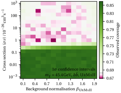
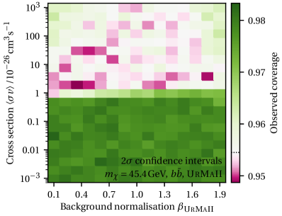
Figure 1: Simulated data for Ursa Major II, demonstrating the coverage of our frequentist intervals for $\left\langle\sigma\!v\right\rangle$ as a function of the true cross section $\left\langle\sigma\!v\right\rangle$ and true background normalisation parameter $\beta_{\textsc{UrMaII}}$. Left: Coverage of nominal “$1\sigma$” confidence intervals, which ideally should contain the true $\left\langle\sigma\!v\right\rangle$ 68.3% of the time (white colour, value denoted by a dotted line in the colour bar). Right: Coverage of nominal “$2\sigma$” intervals, which ideally should contain the true $\left\langle\sigma\!v\right\rangle$ 95.4% of the time. Green parameter values overcover (i.e., confidence intervals are conservative), while pink parameter values undercover, albeit very slightly (less than 1% under-coverage everywhere).

We choose 21 cross sections between $10^{-29}$ and ${10}^{-23}\text{\,}\mathrm{c}\mathrm{m}^{3}\mathrm{/}\mathrm{s}$, 15 values of $\beta_{\textsc{UrMaII}}$ between 0.1 and 1.9, and 4 dark masses ($m_{\chi}$= 10.1, 45.4, 209, and 1097 GeV) and perform the coverage test for all 1,260 possible combinations of these parameters (all in all, 12 million mock data sets). Figure 1 shows the resulting coverage for a dark matter mass $m_{\chi}=45.4$ GeV (other choices of mass give a similar picture). Each rectangle in the figure corresponds to $10^{4}$ data sets where the true values of $\left\langle\sigma\!v\right\rangle$ and $\beta_{\textsc{UrMaII}}$ are those at the centre of the rectangle. We observe over-coverage for small values of $\left\langle\sigma\!v\right\rangle$ (i.e. conservative limits), and essentially exact coverage once $\left\langle\sigma\!v\right\rangle$ increases beyond a threshold. Coverage holds for every possible value of $\beta_{\textsc{UrMaII}}$ between 0.1 and 1.9. This test not only establishes coverage for different true values of the cross section, but also for different possibilities for the background normalisation.

This is made clearer in Fig. 2, which shows the observed coverage as a function of $\left\langle\sigma\!v\right\rangle$, averaged over values of the true (simulated) $\beta_{\textsc{UrMaII}}$, for each choice of mass we tested (narrow shaded bands around each line give the standard deviation of our estimate of the coverage). The 15 values of $\beta_{\textsc{UrMaII}}\in[0.1,1.9]$ are weighted equally in the average. Horizontal dashed lines are at 0.683 and 0.954, the values of exact coverage. We can see that the nominal $1\sigma$ limits overcover (i.e., are conservative) for $\left\langle\sigma\!v\right\rangle$ values smaller than $3\text{\times}{10}^{-27}\text{\,}\mathrm{c}\mathrm{m}^{3}\mathrm{/}\mathrm{s}$ (for $m_{\chi}=$10\text{\,}\mathrm{GeV}$$) or smaller than ${10}^{-25}\text{\,}\mathrm{c}\mathrm{m}^{3}\mathrm{/}\mathrm{s}$ (for $m_{\chi}=$1096\text{\,}\mathrm{GeV}$$) (depending on the mass), which is the range of cross section of interest to us. For larger cross sections (which are irrelevant for our purposes), coverage is close to exact, with a possible small amount of undercoverage for the largest mass value we tested.

The picture for the $2\sigma$ limits is similar, exhibiting overcoverage (i.e., conservatism) for $\left\langle\sigma\!v\right\rangle$ values smaller than ${10}^{-26}\text{\,}\mathrm{c}\mathrm{m}^{3}\mathrm{/}\mathrm{s}$ (for $m_{\chi}=$10\text{\,}\mathrm{GeV}$$) and smaller than ${10}^{-24}\text{\,}\mathrm{c}\mathrm{m}^{3}\mathrm{/}\mathrm{s}$ (for $m_{\chi}=$1096\text{\,}\mathrm{GeV}$$), with exact coverage above these values.

In summary, we conclude that the coverage properties of our frequentist intervals are excellent.

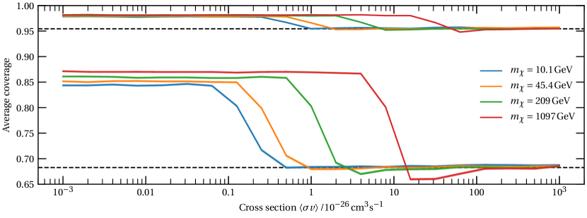
Figure 2: Coverage of confidence intervals for $\left\langle\sigma\!v\right\rangle$, averaged over the true value of the background normalisation parameter $\beta_{\textsc{UrMaII}}$, as a function of true cross section for several values of dark matter mass, $m_{\chi}$. The upper and lower sets of lines show $1\sigma$ and $2\sigma$ confdience intervals. Shaded bands around the lines (barely visible) show the standard deviation of our estimate of the coverage. Horizontal dashed lines are at 0.683 and 0.954, the values of exact coverage.

3 Results and discussion

In this section, we present and discuss the results of the Ret II analysis as well as the global analysis involving all 27 dSphs. We use various algorithms for the different computational tasks (integration, sampling, maximization). We use MultiNest [89, 90, 91] for calculating the Bayesian evidence. MultiNest is a nested sampling algorithm [92], closing in on the regions of highest likelihood in nested shells. In MultiNest, these shells are approximated with an ellipsoidal decomposition, and contain sets of live points that are updated in each iteration step by replacing the point with the lowest likelihood by a new one from the prior distribution under the constraint that is has a larger likelihood value.

We use T-Walk [87] for sampling posterior distributions, which is an ensemble Markov Chain Monte Carlo algorithm based on Ref. [93]. It consists of a fixed number of chains, one of which is advanced at each iteration. This selection is random and the proposal distribution for the advancement, which is selected from a pool of different “moves”, depends on the remaining chains.

Finally, Diver [87] is used to map out the profile likelihood (which requires dedicated tools, since the typical Bayesian sampling of the posterior offers insufficient resolution for profile likelihood mapping [94]). It is a differential evolution algorithm [95] and consists of a “population” of parameter points, whose parameter values are its “genes”. The population evolves over time via mutation and crossover (of “genes”), and selection (of the “fittest individuals”, where fitness is measured by the log-likelihood value), hence mimicking the process of natural selection. This heuristically aims at achieving the highest possible “fitness” amongst some of the parameter points, i.e. the maximum likelihood value.

3.1 Analysis of Reticulum II

First, we investigate the WIMP parameter space of mass, $m_{\chi}$, and thermally-averaged annihilation cross section, $\left\langle\sigma\!v\right\rangle$, using only the Ret II data described in Sec. 2.1. The additional nuisance parameters for Ret II are therefore the background scaling, $\beta_{\text{{Ret\leavevmode\nobreak\ II}}}$, and the $J$-factor, $\log_{10}J_{\text{{Ret\leavevmode\nobreak\ II}}}$. Since this part of the study is mainly to illustrate our methodology and since qualitative conclusions from the $\tau^{+}\!\tau^{-}$ and $b\bar{b}$ channels are similar, we restrict our Ret II analysis to the $\tau^{+}\!\tau^{-}$ channel only.

The non-default settings for Diver (NP: $5\text{\times}{10}^{4}$, convthresh: ${10}^{-5}$, jDE: true, lambdajDE: false), MultiNest (nlive: $2\text{\times}{10}^{4}$, tol: ${10}^{-4}$), and T-Walk (sqrtR: $1.001$ with 528 MPI processes) were informed by a previous study using these algorithms [87].

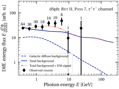
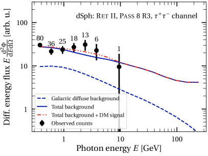
Figure 3: Spectra for 6.5 years of Pass 7 (left) and Pass 8 (right) data for Ret II. We show the observed counts (black circles and numbers) with Poisson error bars, as well as the backgrounds (blue lines) and background plus DM signal (red lines), according to the best-fit parameters in the $\tau^{+}\!\tau^{-}$ channel. The best-fit DM mass is $m_{\chi}=$13.3\text{\,}\mathrm{GeV}$$ (left panel) and $m_{\chi}=$14.2\text{\,}\mathrm{GeV}$$ (right panel).

Since the number of weeks for our data selection is the same as in Ref. [16], we expect to find an indication for a signal using Pass 7 data. This indeed is confirmed by Fig. 3, which shows Pass 7 and Pass 8 (R3) data for Ret II together with the best-fit spectra from the fit that will be discussed later in this section (red lines). In the energy region around a few GeV, there appears to be an excess above the fitted background (blue lines) for Pass 7, which is less prominent for Pass 8. This energy region is therefore able to accommodate an additional signal contribution from DM annihilation. The number of “excess photons” amounts to about 26 photons in Pass 7 and 7 photons in Pass 8 across the whole energy range considered.

The lowest energy bins, on the other hand, place the strongest constraints on the background normalisation, due to the high number of observed counts in them. This is an important consideration for any analysis that simultaneously fits background and signal contributions. The lowest energy bin, i.e. photons with energies around $0.4\text{\,}\mathrm{GeV}$, is more important in Pass 8 than in Pass 7, given that there are 16 additional photons in Pass 8. However, the energy bins in the right half of the bump contain fewer photons in Pass 8 compared to Pass 7.

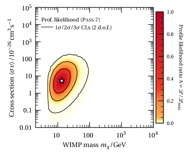
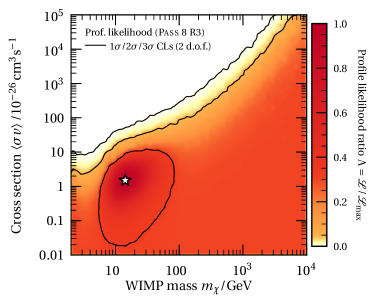
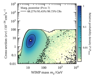
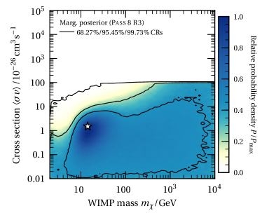
Figure 4: Constraints on WIMP parameters from 6.5 years of Ret II data. We show profile likelihoods (top) and marginal posteriors (bottom), using Pass 7 (left) and Pass 8 (right) data for the $\tau^{+}\!\tau^{-}$ channel and a log-uniform prior on $\left\langle\sigma\!v\right\rangle$. The star denotes the best-fit point. We show two-sided CLs and highest posterior density CRs for profile likelihoods and posteriors, respectively. Note that the posteriors are restricted to the region $\left\langle\sigma\!v\right\rangle_{-26}<100$ due to the prior range on $\left\langle\sigma\!v\right\rangle$.

In Fig. 4, we show profile likelihoods (top panels) and the marginal posteriors (bottom panels) for the WIMP mass and cross section, where the nuisance parameters $\beta_{\text{{Ret\leavevmode\nobreak\ II}}}$ and $\log_{10}J_{\text{{Ret\leavevmode\nobreak\ II}}}$ have been profiled out and marginalised over, respectively. The profile likelihood for Pass 7 (top left panel) shows a stronger than $3\sigma$ preference for a DM signal. Such a preference is reduced to $1\sigma$ when using Pass 8 data (top right panel).

As we saw in Fig. 3, the energy region of the putative excess results in a preferred value for the WIMP mass $m_{\chi}$. The inclusion of the likelihood for $J_{\text{{Ret\leavevmode\nobreak\ II}}}$, on the other hand, allows for a direct inference on $\left\langle\sigma\!v\right\rangle$, which includes both the uncertainty in the $J$-factor measurement and that from the Poisson likelihood.

The best-fit parameters of the WIMP properties for the $\tau^{+}\!\tau^{-}$ channel in Pass 7 (Pass 8) data are $\widehat{m}_{\chi}=$13.3\text{\,}\mathrm{GeV}$$ and $\widehat{\left\langle\sigma\!v\right\rangle}_{-26}=$5.48$$ ($\widehat{m}_{\chi}=$14.2\text{\,}\mathrm{GeV}$$ and $\widehat{\left\langle\sigma\!v\right\rangle}_{-26}=$1.55$$). The best-fit mass values are similar for Pass 7 and Pass 8 because the excess is around the same energy region for both data sets. Since the number of “excess photons” in this region is higher for Pass 7, it is also not surprising that the best-fit parameter for $\left\langle\sigma\!v\right\rangle$ reflects this.

While the statistical interpretation of the posterior credible regions (CRs) in a Bayesian analysis is different from the confidence levels (CLs) in a frequentist understanding, the Bayesian posteriors in the bottom panels of Fig. 4 paint a qualitatively similar picture in terms of the statistical conclusions. The Pass 7 marginal posterior distribution shows a very slight presence of an additional signal to the background; the 68.27% CR (corresponding to $1\sigma$ in the Gaussian case) is a closed contour, but the 95.45% CR (corresponding to $2\sigma$ in the Gaussian case) does not exclude the lower prior cut-off. For Pass 8 data (bottom right panel), the 68.27% CR in the same plot extends to most of the parameter space. This region becomes difficult to sample because the posterior distribution flattens out and thus the sampled posterior looks “patchy” in the plot. Comparing the top (frequentist) and bottom (Bayesian) panels, we notice that the Bayesian inference tends to be more conservative, as the marginalisation over the nuisance parameters typically produces wider CRs when compared to profiled likelihood CLs in cases where there is significant “volume effect” in the hidden dimensions (see e.g. Ref. [97]). In light of this result for the Bayesian parameter inference, we do not expect to find Bayesian evidence for the DM signal hypothesis from either data set when we perform a Bayesian model comparison later in this section.

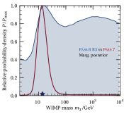
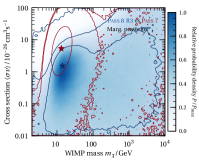
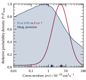
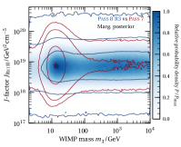
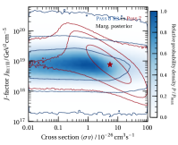
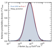
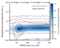
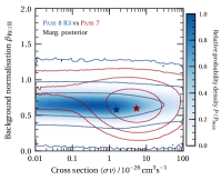
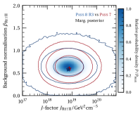
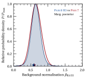
Figure 5: One- and two-dimensional marginal posteriors for Ret II (6.5 years, $\tau^{+}\!\tau^{-}$ channel, log-uniform prior on $\left\langle\sigma\!v\right\rangle$), showing the 68.27%/95.45%/99.73% credible regions from Ret II data. The red colour maps, contours and shaded regions are for Pass 7, while the blue contours are for Pass 8. Red and blue stars indicate the best-fit points for the respective data sets.

In Fig. 5, we show all one- and two-dimensional marginal posteriors for Pass 7 vs Pass 8 data and a log-uniform prior on $\left\langle\sigma\!v\right\rangle$. This illustrates again that, in Pass 7, there is a clearly preferred range for $\left\langle\sigma\!v\right\rangle$, while in Pass 8 there is not. However, the regions of highest posterior density (HPD) in both data sets are roughly in the same regions in parameter space as each other and the highest profile likelihood regions in the frequentist analysis. This means that the priors do not have a large impact on the analysis and the parameter regions singled out by the analysis are mostly data-driven.

Figure 5 is also useful for visualising correlations between parameters, such as the expected anti-correlation between $J_{\text{{Ret\leavevmode\nobreak\ II}}}$ and $\left\langle\sigma\!v\right\rangle$ from Pass 7 data, where a signal is preferred. This is because the DM signal is proportional to the product of both. Furthermore, the one-dimensional marginalised posteriors summarise the constraints that can be put on the individual parameters. Regarding $m_{\chi}$ and $\left\langle\sigma\!v\right\rangle$, they follow the expected behaviours in case of a strong (Pass 7) or weak (Pass 8) preference for a signal, while $J_{\text{{Ret\leavevmode\nobreak\ II}}}$ behaves as expected for a constrained nuisance parameter.

We note an interesting result for the background normalisations: In Pass 7 (Pass 8), we have a best-fit value of $\hat{\beta}_{\text{{Ret\leavevmode\nobreak\ II}}}\approx 0.60$ ($\hat{\beta}_{\text{{Ret\leavevmode\nobreak\ II}}}\approx 0.58$). These values are considerably lower than the all-sky value of $1$, which lies just outside the 95% CRs for the resulting posterior distributions. This implies that the background in the immediate vicinity around Ret II is quite a bit lower than the average in a larger surrounding area. Since we introduced the scaling parameters $\beta_{k}$ to account for the possibility of a local discrepancy of the background with respect to the reference global background model, it will be interesting to compare results for a larger number of dSphs in the next section. The shapes of the marginal posteriors for $\beta_{\text{{Ret\leavevmode\nobreak\ II}}}$ are also similar, with the marginalised posterior using Pass 7 data being slightly broader than in Pass 8.

While the background components’ spectral shapes are slightly different between Pass 7 and Pass 8, Fig. 3 shows that the best-fitting models of the total background are nearly identical in the region of the excess (between about $1$ and $10\text{\,}\mathrm{GeV}$). This points to the conclusion that the Pass 7–Pass 8 difference arises not because of a different background fit, but rather because of a genuine reduction in the number of excess photons in going from Pass 7 to Pass 8.

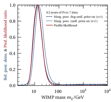
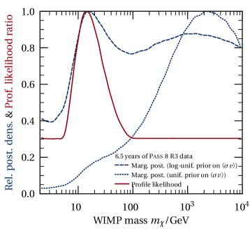
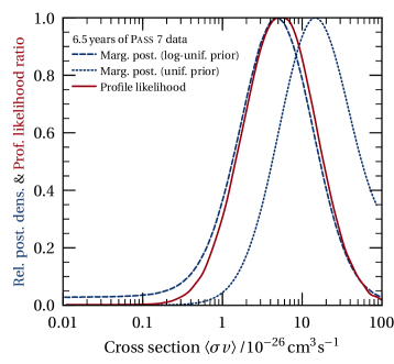
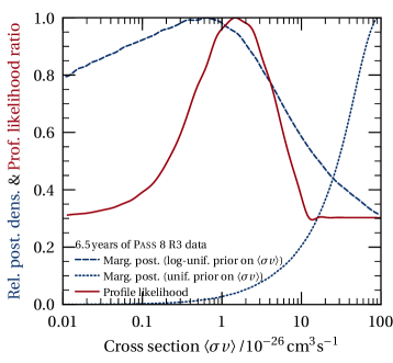
Figure 6: One-dimensional marginal posteriors (blues lines) and profile likelihoods (red lines) for $m_{\chi}$ (top) and $\left\langle\sigma\!v\right\rangle$ (bottom). We show these for 6.5 years of Pass 7 (left) and Pass 8 (right) data (Ret II, $\tau^{+}\!\tau^{-}$ channel).

Figure 6 shows the one-dimensional marginal posterior distributions and profile likelihoods for $m_{\chi}$ and $\left\langle\sigma\!v\right\rangle$ and the two priors on $\left\langle\sigma\!v\right\rangle$ adopted in this study. For a log-uniform prior on $\left\langle\sigma\!v\right\rangle$, the resulting CRs peak at a similar location in both Pass 7 and Pass 8. However, this is not the case when using a uniform prior on $\left\langle\sigma\!v\right\rangle$. In the left panel of Fig. 6 we can see that, for Pass 7, the modes of the profile likelihood and posteriors agree rather well, even though the mode for $\left\langle\sigma\!v\right\rangle$ using a uniform prior on $\left\langle\sigma\!v\right\rangle$ is found at a higher value compared to the other two, reflecting the higher prior density for larger $\left\langle\sigma\!v\right\rangle$ values under the uniform prior on this quantity. For Pass 8 (right panel), on the other hand, the main modes of the marginal posteriors for $m_{\chi}$ and $\left\langle\sigma\!v\right\rangle$ (using a uniform prior on $\left\langle\sigma\!v\right\rangle$) get both shifted to higher values compared to the profile likelihoods and marginal posteriors using a log-uniform prior on $\left\langle\sigma\!v\right\rangle$. Also, the marginal posteriors with the two different priors are quite different from each other, indicating strong prior dependence as a consequence of less constraining data. This is due to the absence of a strong preference for a signal in Pass 8 and the higher prior weight on larger values for the cross section affects the posterior on the WIMP parameters. While a significant part of the posterior density is concentrated around the best-fit points for a log-uniform prior on $\left\langle\sigma\!v\right\rangle$, a uniform prior on $\left\langle\sigma\!v\right\rangle$ dominates the posterior density in Pass 8 and causes the marginal posterior of the cross section (and hence also the mass) to move to higher values.

3.1.1 Model comparison for Reticulum II

Table 2: Bayes factors for comparing a background-only model with a model including an additional DM signal from $\tau^{+}\!\tau^{-}$ channel annihilation (using 6.5 years of Ret II data). A positive (negative) value of $\ln\left(\mathcal{B}_{10}\right)$ indicates evidence in favour of (against) the model with an additional DM signal. The value of $\mathcal{B}_{10}$ gives the posterior odds between the DM model and the background only model if each model has equal prior probability.

	Pass 7		Pass 8
Prior on $\left\langle\sigma\!v\right\rangle$	uniform	log-uniform	uniform	log-uniform
Bayes factor $\ln\left(\mathcal{B}_{10}\right)$	$1.61\pm 0.02$	$1.92\pm 0.02$	$-0.65\pm 0.02$	$-0.12\pm 0.02$
Bayes factor $\ln($$\mathcal{B}_{10}$	5:1	7:1	$-$1:2	$-$1:1

To quantify the preference (or lack thereof) for a DM signal contribution to the gamma-ray spectrum of Ret II, we compute the Bayesian evidence for the background-only and the background-plus-signal model. The conceptual difference between Bayesian model comparison and frequentist hypothesis testing is that the latter can only reject the null hypothesis, while the former can show a preference for a simpler model whenever the added complexity of the more complicated model is not warranted by the data. In other words, the Bayesian model comparison framework includes an automatic Occam’s razor effect.

We define the background-only model via setting $\left\langle\sigma\!v\right\rangle=0$, meaning that the DM mass parameter becomes non-identifiable. The resulting Bayes factor for both data sets, Pass 7 and Pass 8, as well as the two adopted choices of prior on $\left\langle\sigma\!v\right\rangle$ are given in Table 2.

We use a commonly applied scale for categorising how strongly one model is favoured over the other, dating back to Jeffreys [98, 99], with the nomenclature adopted from Ref. [72]. This “Jeffreys’ scale” has thresholds at $\left|\ln\left(\mathcal{B}_{10}\right)\right|=1.0$, $2.5$, and $5.0$, which we call respectively weak, moderate, and strong evidence. From Table 2, we can see that only Pass 7 data gives weak evidence (i.e. a Bayes factor of more than 3:1) for the DM hypothesis regardless of the adopted prior. On the other hand, the model comparisons using Pass 8 neither favour a DM signal, as already anticipated in the previous section, nor do they favour the background-only model. The Pass 8 data are simply insufficiently informative to reach a conclusion either way.

We notice that, as expected, the outcome of the Bayesian model comparison is much more conservative than what would be obtained using a $p$-value frequentist approach [100]: even in the case of Pass 7 data, which gives a more than $3\sigma$ significance for a non-zero $\left\langle\sigma\!v\right\rangle$, the Bayes factor for a log-uniform prior is only 7:1, shy of the threshold for even moderate evidence at 12:1. This is an example of a well known statistical phenomenon called the Lindley paradox: the outcome of hypothesis testing and Bayesian model comparison differs (even asymptotically for large amount of data), because the two approaches ask fundamentally different questions (see Refs [86, 73] for a detailed discussion and further references).

In any case, the model comparison further quantifies the mostly qualitative findings that emerged so far in this section. Confirming previously proposed explanations for the difference in significance for a potential excess in Ret II [17, 32], we find that this is due to the differences in Pass 7 and Pass 8 since the results of the Bayesian and the frequentist analysis agree when using Ret II data based on the same selection criteria.

3.1.2 Posterior predictive distributions for signal strengths in other dwarfs

After having re-visited the purported gamma-ray excess in Ret II, we investigate how our conclusions might change when considering the other dSphs, both in terms of WIMP parameter constraints and model selection outcome. Our starting point is to note that physical consistency requires that the WIMP parameters must be the same across all dSphs. Therefore, given a possible excess from Ret II, it is helpful to quantify the probability that an excess due to the same dark matter candidate will be seen in other dwarfs. One possibility is to use the best-fit WIMP parameters from Ret II to establish the strength of the DM signal in other dSphs. However, this approach neglects the uncertainties in the WIMP parameters as well as the uncertainties arising from the $J$-factor and background rescaling for the dwarf for which the prediction is being made. It also does not quantify the probability of achieving a statistical significant measurement in another dwarf.

In this section, we introduce the posterior predictive distribution (PPD) as a tool to precisely quantify the probability of seeing a DM-related signal in one dSph, conditional on the observation in another one (in this case, Ret II). The same approach can also be used to make predictions for future observations of the same dwarf, i.e. over longer integration times.

The advantage of this approach is three-fold: firstly, the ensuing predicted distribution is a probability distribution for the yet unobserved data, which fully accounts for all relevant sources of uncertainty. Secondly, this approach clarifies that not seeing a DM signal from a dwarf where one would not expect it (e.g. because the $J$-factor is too low) is not an indication against the DM model. Indeed, the contribution to the Bayes factor from such a dwarf is null: if the distribution of data under both the background-only model and the background-plus-signal model are observationally indistinguishable, then making the observation is not going to teach us anything about the relative viability of each model. Finally, PPDs indicate the most promising targets to improve the model comparison result, for example to test the DM model further. A natural extension of PPD is Bayesian decision theory and experimental design, which we do not however pursue further in this work (see Ref. [101] for an example and discussion). More generally, it is important to note that the PPD can be based on posterior samples from any experimental search, not just dSphs.

The PPD for any observable $D$ (which might be future or not-yet-analysed data), given previously analysed data $d$, is

$$p\left(D\,\middle|\,d\right)=\int_{\Theta}\!p(D,\boldsymbol{\theta}|d){\mathrm{d}}\boldsymbol{\theta}=\int_{\Theta}\!p\left(D\,\middle|\,\boldsymbol{\theta},\,d\right)\,p\left(\boldsymbol{\theta}\,\middle|\,d\right)\,\mathrm{d}\boldsymbol{\theta}=\int_{\Theta}\!p\left(D\,\middle|\,\boldsymbol{\theta}\right)\,p\left(\boldsymbol{\theta}\,\middle|\,d\right)\,\mathrm{d}\boldsymbol{\theta}\,,$$ (13)

where $p\left(D\,\middle|\,\boldsymbol{\theta}\right)$ is the likelihood for data $D$ given parameters $\boldsymbol{\theta}$, weighted by the posterior distribution from current data, $p\left(\boldsymbol{\theta}\,\middle|\,d\right)$, and integrated over all values for the parameters, $\boldsymbol{\theta}\in\Theta$. One can easily see that this generalises the “best fit prediction”, obtained directly from the best-fit estimate for $\boldsymbol{\theta}$, which is in particular appropriate if the uncertainty on $\boldsymbol{\theta}$ is relevant. The best-fit prediction is recovered from (13) by setting $p\left(\boldsymbol{\theta}\,\middle|\,d\right)=\delta(\boldsymbol{\theta}-\boldsymbol{\hat{\theta}})$, where $\boldsymbol{\hat{\theta}}$ is the maximum-likelihood estimator of the parameters.

To obtain the PPDs, we select $5\text{\times}{10}^{5}$ random samples out of the equally weighted posterior samples from the analysis of 6.5 years of Pass 7 data using Ret II only. We then generate a realisation of background and DM signal counts for each dSph by drawing them from Poisson distributions with rates given by (3). In order to do so, we require values for the $J$-factor and background normalisation entering the Poisson rate for the dwarf for which the prediction is made. To obtain these, we draw random samples from informative prior distributions: for the $J$-factors, we draw $J$-factor samples directly from the posterior samples supplied in the auxiliary material of Ref. [41].

For the background normalisations, we draw samples from a normal distribution with mean 1, expecting that the background should not need any rescaling on average. The value of the standard deviation, 0.27, was obtained from the posterior obtained by combining all background normalisation parameters $\beta_{k}$ in the global analysis in Sec. 3.2. This represents the observed spread of the background scaling parameter across the 27 dwarfs in the Pass 8 (R3) data set for 11 years of Fermi-LAT observations. As this procedure averages over all dwarfs, it is a more conservative approach than trying to obtain such a prior based on data from each dSph individually.

Figure LABEL:fig:predpost demonstrates how the PPDs conditional on data from one dSph (Ret II) can be used as a diagnostic tool to identify discrepancies between the predicted vs the observed data in the other dSphs and with a larger amount of data, thus identifying the most promising targets for analysis. The figure shows predictions for the spectra (left panel) of the background-only model (filled regions) and for the background-plus-signal model (empty regions) in six different dSphs after 11 years of Pass 8 observations, conditional on the posterior samples from the Pass 7 analysis of Ret II only, adopting a log-uniform prior on $\left\langle\sigma\!v\right\rangle$. We show the PPDs for the three classical and three ultrafaint dSphs with the highest median $J$-factors as examples for the discussion. From a Bayesian model averaging perspective, for each dwarf one could obtain an averaged prediction by summing the two models’ PPDs with weight given by each model’s posterior probability. Given that the outcome of the Bayesian model selection in the previous section was essentially inconclusive, for non-informative priors for each model the models’ posterior probabilities are almost equal. Therefore, a model-averaged prediction would be an approximately equal mixture of the PPDs for each separate model.

We observe in general that, after accounting for all uncertainties, the 68% regions of the PPD predictions for the background-only and for the signal-plus-background model overlap for all energy bins and all dwarfs shown here. This means that a detection of a dark matter signal in these dwarfs would rely on a fortuitous upwards fluctuation of the signal (or downward fluctuation of the background). This is true even for the dSphs with the largest median $J$-factors, Ursa Major II and Segue 1, which exhibit the more prominent “bump” in the background-plus-signal model in the region of the putative excess between $1\text{\,}\mathrm{GeV}$ and $10\text{\,}\mathrm{GeV}$. We also see some downward fluctuations of the observed counts in some energy bins when compared to the background-only predictions, in case of Ursa Minor even outside the 95% predicted probability band. This indicates that the prior on the background parameter disagrees with the data for this particular dSph. In fact, the global analysis revealed that e.g. the best-fit parameter is $\hat{\beta}_{\textsc{UrMi}}=0.47$, i.e. noticeably lower than the reference value of 1.

A more quantitative way of assessing how promising a dSph is in terms of detecting a dark matter signal is the predicted distribution for the signal-to-noise ratio (SNR) in the background-plus-signal model. The SNR for the new dwarf, conditioned on Ret II data, is computed according to the prescription in Ref. [31, Eq. 18]. That study introduces a test statistic $T$ which is shown to have more power than any other at distinguishing a dark matter signal from background. The SNR is a measure of expected detection significance when using this test statistic to search for a signal. It is defined as

$$\text{SNR}\equiv\frac{\mathrm{E}[T\mid H_{1}]-\mathrm{E}[T\mid H_{0}]}{\mathrm{Std}[T\mid H_{0}]}\,,$$ (14)

where $\mathrm{E}[T\mid H_{1}]$ is the expected value of the test statistic under the signal-plus-background hypothesis, while $\mathrm{E}[T\mid H_{0}]$ and $\mathrm{Std}[T\mid H_{0}]$ are the expected value and standard deviation of the test statistic under the background-only hypothesis. Following Ref. [31, Eq. 18], the SNR for a dSph is computed using $\text{SNR}^{2}=\sum_{i,j}(s^{\text{DM}}_{i,j})^{2}\left/b_{i,j}\right.$, where the sum is over spatial and energy bins for the dSph and $b_{i,j}\equiv\lambda_{i,j}-s^{\text{DM}}_{i,j}$ (see Sec. 2).

The resulting distributions and highest-posterior density CRs for the SNRs are shown in the right panel of Fig. LABEL:fig:predpost in order of decreasing predicted median SNR (from top to bottom). Notice that given our definition of SNR, a value of $\text{SNR}>5$ would correspond to a $5\sigma$ detection (assuming a Gaussian distribution of $T$ under the background-only hypothesis). While the maximum of the predictive distribution is in all cases above unity (and often above a value of 5, corresponding to a $5\sigma$ detection), the predictive distribution has very long tails as a consequence of the uncertainties in the $J$-factor and background normalisation, which are fully accounted for in the prediction. There is hence a large fractional probability that the SNR will be smaller than unity and that any signal will be undetectable. We can thus classify each dwarf in terms of the probability to obtain a detection (defined as an SNR value larger than 5), which we call the “discovery probability”. This is simply the integrated posterior predictive probability density for $\text{SNR}>5$. Another measure of the chance of a dark matter detection is the 95% lower limit from the PPD for the SNR. This gives the value of the SNR above which lies 95% of the predicted probability density.

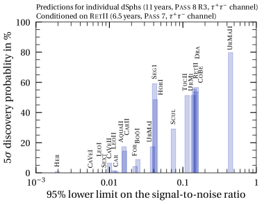
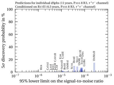
Figure 7: Posterior predictive probability of making a detection of a DM signal at more than $5\sigma$ significance in another dwarf, including all relevant sources of uncertainty, conditional on Ret II data. We show the results, sorted by their lower SNR limit, conditioned on 6.5 years of Pass 7 (left) and Pass 8 (right) Ret II data ($\tau^{+}\!\tau^{-}$ channel, log-uniform prior on $\left\langle\sigma\!v\right\rangle$). The probability of detection drops dramatically from Pass 7 to Pass 8 data.

We show these values in Fig. 7, conditioned on 6.5 years of Ret II data in Pass 7 (left panel) and Pass 8 (right panel) for the $\tau^{+}\!\tau^{-}$ channel and a log-uniform prior on $\left\langle\sigma\!v\right\rangle$. The individual dSphs are sorted by the 95% lower limit on the SNR. Conditional on Pass 7 data, the probability of a discovery in an individual dSph is larger than 50% in seven of them. The highest individual discovery probability occurs for Ursa Major II with a value of about 80%. Note that the six  Sphs with long tails (cf. Sec. 2.3) do not appear in the plot because they have much lower limits with vanishingly low $\text{SNR}<10^{-12}$. However, Pegasus III and Draco II still show a fairly reasonable discovery probability of 17% and 18%, respectively.

We can also evaluate the probability that at least one of the dSphs yields a $5\sigma$ or higher detection. If each dwarf were independent, the probability of a detection in any one of the $N=27$  dwarfs (ignoring the “look-elsewhere effect”) would simply be given by

$$P_{\text{det}}=1-\prod_{k=1}^{N}\,\Big{(}1-\int_{5}^{\infty}\!p\left(\text{SNR}_{k}\,\middle|\,d\right)\,\mathrm{d}(\text{SNR}_{k})\Big{)}\,,$$ (15)

where $d$ are the data that the PPD is conditioned upon, and $p$ is the PPD for the SNR in dwarf $k$. However, the signal is of course fully correlated in all dSphs since, in the presence of dark matter, the WIMP mass and cross section are exactly the same for all dSphs. Therefore, we must instead estimate the probability of making a detection in at least one dwarf numerically, as the fraction of posterior samples for which $\text{SNR}>5$ in at least one dwarf, i.e. the SNR surpasses the detection threshold. Doing so using the Pass 7 posterior samples results in a probability of 90%. This means that, conditional on Pass 7 Ret II data, there is a 90% probability that at least one of the other dwarfs yields a $5\sigma$ detection.

Conditional on 6.5 years of Pass 8 data from Ret II, on the other hand, there is no strong preference for a DM signal and it is therefore not surprising that the predicted SNR in the other dSphs will generally not yield a detection (right panel of Fig. 7). However, a few of the dwarfs, such as Ursa Major II, Horologium I or Segue 1, still have a sizeable probability for an individual detection. Still, the probability to make a detection in at least one dSph, conditional on 6.5 years of Ret II data in Pass 8, drops to 24%. The six dwarfs with long tail have again a much lower limit on the SNR than the others, with Pegasus III and Draco II showing comparable discovery probabilities to other dSphs (2.4% and 5.3%, respectively).

PPDs can therefore be used as a tool to determine which dSphs are likely to result in a detection (or rule out a model, depending on the statistical question being asked). While a full global analysis is always desirable, it can become computationally very expensive as more dSphs are added to the likelihood, perhaps with additional nuisance parameters. In this case, a potential solution is to include only the “most promising” dSphs such that the outcome of the analysis is ideally approximately as strong as the result of a global, complete analysis. While the relevance of a dSph might be determined by, e.g., the highest $J$-factor or their likelihood contribution, PPDs can help identify these systems in a more statistically principled way, while at the same time accounting for all relevant uncertainties in the prediction. We use the findings of this section to inform our choices for the Bayesian model comparison in the global analysis.

3.2 Global analysis of 27 dwarfs

We now turn to our findings from a global analysis, using 11 years of Pass 8 (R3) data for 27 dwarfs in the likelihood function. Our analysis has a total of 56 parameters: the background normalisations and $J$-factors for each of the dSphs, plus $m_{\chi}$ and $\left\langle\sigma\!v\right\rangle$. For parameter estimation, we increase the number of parallel chains for T-Walk (sqrtR: $1.01$ with 2016 MPI processes), resulting in around 200 million equally weighted samples for each channel, and use more demanding settings for Diver (NP: ${10}^{5}$, convthresh: ${10}^{-7}$, jDE: true, lambdajDE: false).

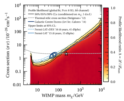
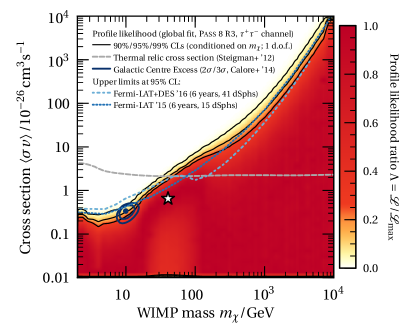
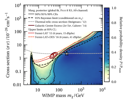
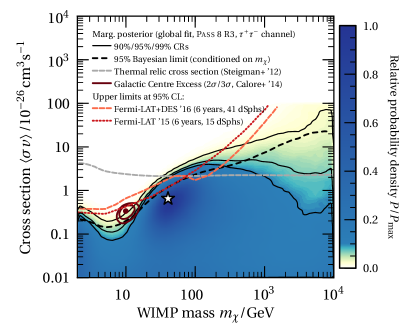
Figure 8: Global analyses using 11 years of Pass 8 data for 27 dwarfs. We show profile likelihoods (top) and marginalised posteriors (bottom) for the $\tau^{+}\!\tau^{-}$ (left) and $b\bar{b}$ (right) channels. The star denotes the best-fit point for a given channel. We compare our results with the thermal relic cross section [83], previous limits [18, 23], and parameters associated with the purported Galactic Centre excess [39]. Note that the posteriors are restricted to the region $\left\langle\sigma\!v\right\rangle_{-26}<100$ due to the prior range on $\left\langle\sigma\!v\right\rangle$ for the Bayesian analysis.

The DM parameter constraints from the global analysis, separately considering the $\tau^{+}\!\tau^{-}$ and $b\bar{b}$ channels, are shown in Fig. 8. The top row shows results from the profile likelihood (where the likelihood has been maximised over the nuisance parameters), while the bottom row shows the Bayesian posterior (where nuisance parameters have been marginalised over). We also display for reference the thermal relic cross section [83] and limits from previous analyses at 95% CL. In the top panels, the confidence limits have been obtained conditional on the value of the mass, in order to make them exactly comparable to those obtained by the Fermi-LAT Collaboration [18, 23]. The best-fit WIMP parameters in the global fit for the $\tau^{+}\!\tau^{-}$ ($b\bar{b}$) channel are $\widehat{m}_{\chi}=$40.5\text{\,}\mathrm{GeV}$$ and $\widehat{\left\langle\sigma\!v\right\rangle}_{-26}=$0.67$$ ($\widehat{m}_{\chi}=$210\text{\,}\mathrm{GeV}$$ and $\widehat{\left\langle\sigma\!v\right\rangle}_{-26}=$2.23$$).

For WIMP masses below about $100\text{\,}\mathrm{GeV}$, we obtain stronger limits compared to previous frequentist analyses. As a consequence, we can exclude the best-fit DM parameter values for the $b\bar{b}$ channel DM interpretation of the Galactic Centre (GC) excess [102, 103, 104, 105, 39] at more than 99% CL. For the $\tau^{+}\!\tau^{-}$ channel, the GC excess best fit point can be excluded at the 95% CL. This improves the exclusion strength of dSphs compared to previous studies [e.g. 106, 23, 107].

The Bayesian analysis (bottom panels of Fig. 8) disfavours the GC excess DM interpretation even more strongly. Indeed, we notice that for low WIMP mass the Bayesian credible region is noticeably more constraining than the profile likelihood. The best-fit point and part of the associated confidence regions for the DM interpretation of the GC excess from Ref. [39] is outside the 99% credible regions in the Bayesian analyses for both channels (bottom panel of Fig. 8). Recall that our choice of prior lower boundary for the Baysian analysis is conservative, i.e. yields looser upper limits than would be obtained by increasing the prior range at the low end. Notice that the Bayesian contours in the bottom panels are two-dimensional credible regions, which cannot be directly compared with the one-dimensional profile likelihood limits in the upper panels (which instead condition on the value of the mass). To facilitate a direct comparison, we also compute a “Bayesian 95% limit” on the cross section (shown as black dashed line in the bottom panel of Fig. 8). This is obtained by integrating the posterior conditional on the given value of $m_{\chi}$, in order to mimic the procedure used for the frequentist conditional CL. This Bayesian limit is somewhat closer to the frequentist 95% CL than the corresponding CR for lower WIMP masses, but still overall stronger than the frequentist result.

In our analysis of Ret II, we observed that the best-fit value for the background normalisation, $\hat{\beta}_{\text{{Ret\leavevmode\nobreak\ II}}}=0.58$ (for Pass 8 data), was noticeably lower than the reference value of $\beta_{\text{{Ret\leavevmode\nobreak\ II}}}=1$ in both Pass 7 and Pass 8. In the global analysis, we find again that $\hat{\beta}_{\text{{Ret\leavevmode\nobreak\ II}}}\approx 0.67<1$. There seems to be a slight re-absorption of the excess photons in Ret II by the higher background component as non-detections in other dwarfs force the value of $\left\langle\sigma\!v\right\rangle$ ($m_{\chi}$) to lower (higher) values than in the Ret II-only analysis. These WIMP parameters require a slightly higher background normalisation to provide a good fit the shape of the Ret II spectrum. Regarding the other dSphs, the 95% HPD region 11 of them contains $\beta_{k}=1$, for 15 of them it lies below $\beta_{k}=1$, and only for Leo V is lies above $\beta_{k}=1$.

Combining the posteriors for all $\beta_{k}$ into one set results in a distribution that allows us to estimate the mean and spread of the $\beta_{k}$. We find that the samples of all dwarfs combined have a posterior mean and standard deviation of 0.76 and 0.27, respectively. Similar to how we used this information in Sec. 3.1.2, the mean, standard deviation, or both may be used to inform prior choices in future studies with comparable background modelling.

Tabulated exclusion limits, profile likelihood and marginal posterior density maps for Fig. 8 and the limits presented in Appendix A are freely available on Zenodo [108].

Table 3: Bayes factors for comparing a background-only model with a model including an additional DM signal (11 years of Pass 8 data; we use the most promising 10 dSphs, selected using the PPD of their SNR). A positive (negative) value of $\ln\left(\mathcal{B}_{10}\right)$ indicates evidence in favour of (against) the model with an additional DM signal. The value of $\mathcal{B}_{10}$ gives the posterior odds between the DM model and the background only model if each model has equal prior probability.

Prior on $\left\langle\sigma\!v\right\rangle$	$\tau^{+}\!\tau^{-}$ channel		$b\bar{b}$ channel
	uniform	log-uniform	uniform	log-uniform
Bayes factor $\ln\left(\mathcal{B}_{10}\right)$	$-0.88\pm 0.05$	$-$$0.01\pm 0.05$	$-1.09\pm 0.05$	$-$$0.02\pm 0.05$
Bayes factor $\ln($$\mathcal{B}_{10}$	$-$1:2	$-$1:1	$-$1:3	$-$1:1

Finally, we also performed a model comparison by calculating Bayes factors for the two hypotheses with MultiNest. Obtaining reliable estimates for the Bayesian evidence proved difficult due to the relatively large dimensionality of the parameter space (the efficiency of MultiNest drops quickly above about 30 dimensions [109]). We therefore reduced the dimensionality of the parameter space by making a smaller selection of dSphs, choosing those with a median predicted SNR greater than unity when conditioned on Pass 7 data using the PPD approach in the previous section. These are the following ten dSphs: Coma Berenices, Draco, Horologium I, Reticulum II, Sculptor, Segue 1, Tucana II, Ursa Major I, Ursa Major II, and Ursa Minor. We also use slightly less demanding settings for MultiNest (nlive: $2\text{\times}{10}^{4}$, tol: ${10}^{-3}$). The resulting Bayes factors from this analysis can be found in Table 3. Since we have adopted the most constraining (in terms of predicted SNR) dwarfs in this analysis, we expect it to be close to what would have been obtained by including all of the 27 dwarfs.

Since we found no preference for a signal in the parameter estimation part of the global analysis, it is not surprising that the model comparison finds no evidence for an additional signal either. On the other hand, we obtain only weak evidence against the signal-plus-background model in the $b\bar{b}$ channel (using a uniform prior on $\left\langle\sigma\!v\right\rangle$).

The outcome of the model comparison is inconclusive, as there is only weak evidence against the signal-plus-background model for the $b\bar{b}$ channel and a uniform prior. Compared the Ret II section, the trend that a uniform prior on $\left\langle\sigma\!v\right\rangle$ gives lower Bayes factors continues also in the global analysis. Indeed, since the WIMP parameter space always allows for the possibility of having an essentially irrelevant gamma-ray signal, the signal-plus-background model can only be disfavoured compared to the background-only model due to the Occam’s razor effect. This happens when the region of WIMP parameter space resulting in a negligible gamma-ray signal from DM is only a small fraction of the prior volume – the Occam’s razor effect penalising models with “wasted” parameter space. The size of the prior volume of the WIMP parameters is therefore the most important ingredient that would allow the odds to swing in favour of the background-only model. This also explains the trend we observe with the two adopted priors since this fraction is smaller for a prior uniform in $\left\langle\sigma\!v\right\rangle$ than for a prior uniform in the log of $\left\langle\sigma\!v\right\rangle$.

4 Conclusions

We have revisited dark matter searches in dSphs in a systematic way, comparing Bayesian and frequentist methods in the largest dSph sample and highest-exposure search performed to date. When looking for a signal while only having imperfect knowledge of background, relevant sources of uncertainties should be accounted for in the analysis in order to obtain robust results. We therefore included scaling factors for the Galactic diffuse background component. Since $J$-factors can only be approximated via fitting formulæ or determined from stellar data, it is also important to account for their theoretical and statistical uncertainties. For this analysis, we relied on dwarf spheroidal galaxies with posteriors for their $J$-factors as determined by spectroscopic data. To properly account for uncertainties we adopted these posteriors as priors for the gamma-ray analysis, without resorting to the usual log-normal approximation that can be inaccurate.

Using Ret II as an example, we illustrated our methodology and investigated the differences between Bayesian and frequentist analyses as well as between Pass 7 and Pass 8 (R3) data. We showed that the putative excess is not significant in Pass 8 data in neither Bayesian nor frequentist analyses, while there is evidence in Pass 7 data for a non-zero signal contribution. In line with previous literature, we conclude that the differences in significance of the excess are due to the data sets rather than details of the analysis, since we applied the identical methodology and equivalent data selection criteria. We also introduced the posterior predictive distribution into gamma-ray signal searches as a useful tool to determine the consistency of a potential signal amongst a sample of dwarf spheroidal galaxies. The posterior predictive distribution combines the posterior uncertainties in model parameters with the Poisson fluctuations expected in observations to create predicted data set distributions, clearly highlighting the difference between the background-only and signal-plus-background hypotheses in different dSphs. These can be used to easily and robustly quantify the probability of a future dark matter detection. Our predictive formalism has wide applicability in dark matter searches beyond gamma-ray and dwarf spheroidal galaxy analyses.

In the global analysis of Pass 8 data, which includes 27 dwarfs with measured $J$-factors and 11 years of observations, we did not find any indication for an excess and hence derived upper limits on the dark matter cross section as a function of the WIMP mass. The best-fit parameters associated with a dark matter interpretation of the Galactic Centre excess that remained previously viable are ruled out by the frequentist analysis at 95% confidence level for the $\tau^{+}\!\tau^{-}$ and $b\bar{b}$ channels. The Bayesian analysis excludes the entirety of the $3\sigma$ confidence region for the Galactic Centre excess at more than 99% probability.

The global analysis comprises a total of 56 parameters, which is a fairly high number of dimensions for sampling algorithms. Thanks to using Diver and T-Walk, two dedicated algorithms for profile likelihood mapping and posterior sampling, we could perform parameter estimation without major problems. However, we also saw that calculating the Bayesian evidence for the global analysis with many dwarf spheroidal galaxies can present a challenge that can make a full global analysis prohibitive. We overcame this problem by using information from posterior predictive distributions of the signal-to-noise ratio to select a subset of the most relevant dwarf spheroidal galaxies.

Appendix A Limits on other annihilation channels

In addition to the $b\bar{b}$ and $\tau^{+}\!\tau^{-}$ channels considered in the main text, we provide limits for seven other channels in Fig. 9. Calculation and implementation of each model’s signal prediction is equivalent to Sec. 2.1 (using sqrtR < $1.05$ in T-Walk). We choose $2\text{\,}\mathrm{GeV}$ as the lower edge of the prior on the WIMP mass for final states with masses lower than that value ($e$, $\mu$, $\tau$, $c$, $g$), or at the mass of the particle for the others ($W$, $Z$). Similar to the $b\bar{b}$ and $\tau^{+}\!\tau^{-}$ channels investigated in the main text, both Bayesian and frequentist limits rule out the best-fit points of the DM interpretations of the GC excess.

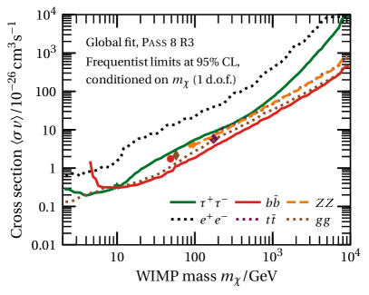
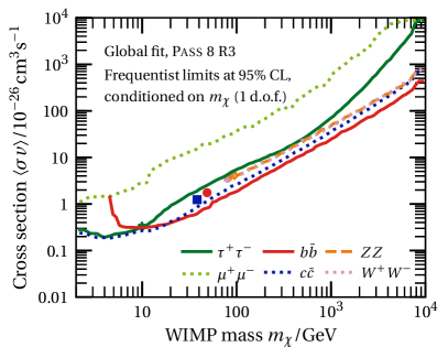
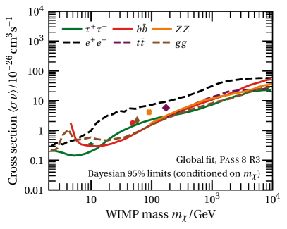
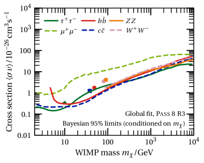
Figure 9: Limits on the cross section $\left\langle\sigma\!v\right\rangle$ for nine different annihilation channels. Top: Frequentist limits at 95% CL (conditioned on $m_{\chi}$; 1 d.o.f.). Bottom: Bayesian 95% limits (conditioned on $m_{\chi}$). Where available, markers with matching colours indicate the best-fit points for the corresponding dark matter interpretation of the Galactic Centre excess in Ref. [39].

All corresponding Bayesian and frequentist limits, profile likelihood maps and marginal posterior density maps corresponding to Fig. 9 are freely available on Zenodo [108], together with a description of the data set and format.

References

- Planck Collaboration et al. [2018] Planck Collaboration, N. Aghanim, Y. Akrami, et al., “Planck 2018 results. VI. Cosmological parameters,” ArXiv e-prints (2018), arXiv:1807.06209.
- Jungman et al. [1996] G. Jungman, M. Kamionkowski, and K. Griest, “Supersymmetric dark matter,” Phys. Rep. 267, 195 (1996), hep-ph/9506380.
- Gaskins [2016] J. M. Gaskins, “A review of indirect searches for particle dark matter,” Contemporary Physics 57, 496 (2016), arXiv:1604.00014 [astro-ph.HE].
- Conrad and Reimer [2017] J. Conrad and O. Reimer, “Indirect dark matter searches in gamma and cosmic rays,” Nature Physics 13, 224 (2017), arXiv:1705.11165 [astro-ph.HE].
- Strigari et al. [2008] L. E. Strigari, S. M. Koushiappas, J. S. Bullock, et al., “The Most Dark-Matter-dominated Galaxies: Predicted Gamma-Ray Signals from the Faintest Milky Way Dwarfs,” ApJ 678, 614-620 (2008), arXiv:0709.1510.
- Atwood et al. [2009] W. B. Atwood, A. A. Abdo, M. Ackermann, et al., “The Large Area Telescope on the Fermi Gamma-Ray Space Telescope Mission,” ApJ 697, 1071 (2009), arXiv:0902.1089 [astro-ph.IM].
- Scott et al. [2010] P. Scott, J. Conrad, J. Edsjö, et al., “Direct constraints on minimal supersymmetry from Fermi-LAT observations of the dwarf galaxy Segue 1,” JCAP 1, 031 (2010), arXiv:0909.3300.
- Abdo et al. [2010] A. A. Abdo, M. Ackermann, M. Ajello, et al., “Observations of Milky Way Dwarf Spheroidal Galaxies with the Fermi-Large Area Telescope Detector and Constraints on Dark Matter Models,” ApJ 712, 147 (2010), arXiv:1001.4531 [astro-ph.CO].
- Essig et al. [2010] R. Essig, N. Sehgal, L. E. Strigari, et al., “Indirect dark matter detection limits from the ultrafaint Milky Way satellite Segue 1,” Phys. Rev. D 82, 123503 (2010), arXiv:1007.4199 [astro-ph.CO].
- Geringer-Sameth and Koushiappas [2011] A. Geringer-Sameth and S. M. Koushiappas, “Exclusion of Canonical Weakly Interacting Massive Particles by Joint Analysis of Milky Way Dwarf Galaxies with Data from the Fermi Gamma-Ray Space Telescope,” Physical Review Letters 107, 241303 (2011), arXiv:1108.2914 [astro-ph.CO].
- Ackermann et al. [2011] M. Ackermann, M. Ajello, A. Albert, et al., “Constraining Dark Matter Models from a Combined Analysis of Milky Way Satellites with the Fermi Large Area Telescope,” Physical Review Letters 107, 241302 (2011), arXiv:1108.3546 [astro-ph.HE].
- Cotta et al. [2012] R. C. Cotta, A. Drlica-Wagner, S. Murgia, et al., “Constraints on the pMSSM from LAT observations of dwarf spheroidal galaxies,” JCAP 4, 016 (2012), arXiv:1111.2604 [hep-ph].
- Mazziotta et al. [2012] M. N. Mazziotta, F. Loparco, F. de Palma, and N. Giglietto, “A model-independent analysis of the Fermi Large Area Telescope gamma-ray data from the Milky Way dwarf galaxies and halo to constrain dark matter scenarios,” Astroparticle Physics 37, 26 (2012), arXiv:1203.6731 [astro-ph.IM].
- Baushev et al. [2012] A. N. Baushev, S. Federici, and M. Pohl, “Spectral analysis of the gamma-ray background near the dwarf Milky Way satellite Segue 1: Improved limits on the cross section of neutralino dark matter annihilation,” Phys. Rev. D 86, 063521 (2012), arXiv:1205.3620 [astro-ph.HE].
- Ackermann et al. [2014] M. Ackermann, A. Albert, B. Anderson, et al., “Dark matter constraints from observations of 25 Milky Way satellite galaxies with the Fermi Large Area Telescope,” Phys. Rev. D 89, 042001 (2014), arXiv:1310.0828 [astro-ph.HE].
- Geringer-Sameth et al. [2015a] A. Geringer-Sameth, M. G. Walker, S. M. Koushiappas, et al., “Indication of Gamma-Ray Emission from the Newly Discovered Dwarf Galaxy Reticulum II,” Physical Review Letters 115, 081101 (2015a), arXiv:1503.02320 [astro-ph.HE].
- Drlica-Wagner et al. [2015] A. Drlica-Wagner, A. Albert, K. Bechtol, et al., “Search for Gamma-Ray Emission from DES Dwarf Spheroidal Galaxy Candidates with Fermi-LAT Data,” ApJ 809, L4 (2015), arXiv:1503.02632 [astro-ph.HE].
- Ackermann et al. [2015] M. Ackermann, A. Albert, B. Anderson, et al., “Searching for Dark Matter Annihilation from Milky Way Dwarf Spheroidal Galaxies with Six Years of Fermi Large Area Telescope Data,” Physical Review Letters 115, 231301 (2015), arXiv:1503.02641 [astro-ph.HE].
- Hooper and Linden [2015] D. Hooper and T. Linden, “On The gamma-ray emission from Reticulum II and other dwarf galaxies,” JCAP 9, 016 (2015), arXiv:1503.06209 [astro-ph.HE].
- Baring et al. [2016] M. G. Baring, T. Ghosh, F. S. Queiroz, and K. Sinha, “New limits on the dark matter lifetime from dwarf spheroidal galaxies using Fermi-LAT,” Phys. Rev. D 93, 103009 (2016), arXiv:1510.00389 [hep-ph].
- Li et al. [2016] S. Li, Y.-F. Liang, K.-K. Duan, et al., “Search for gamma-ray emission from eight dwarf spheroidal galaxy candidates discovered in year two of Dark Energy Survey with Fermi-LAT data,” Phys. Rev. D 93, 043518 (2016), arXiv:1511.09252 [astro-ph.HE].
- MAGIC Collaboration [2016] MAGIC Collaboration, “Limits to dark matter annihilation cross-section from a combined analysis of MAGIC and Fermi-LAT observations of dwarf satellite galaxies,” JCAP 2, 039 (2016), arXiv:1601.06590 [astro-ph.HE].
- Albert et al. [2017] A. Albert, B. Anderson, K. Bechtol, et al., “Searching for Dark Matter Annihilation in Recently Discovered Milky Way Satellites with Fermi-Lat,” ApJ 834, 110 (2017), arXiv:1611.03184 [astro-ph.HE].
- Zhao et al. [2018a] Y. Zhao, X.-J. Bi, P.-F. Yin, and X. Zhang, “Searching for -ray emission from Reticulum II by Fermi-LAT,” Chinese Physics C 42, 025102 (2018a), arXiv:1702.05266 [astro-ph.HE].
- Biswas et al. [2017] S. Biswas, P. Bhattacharjee, P. Majumdar, et al., “Constraints on dark matter models from the observation of Triangulum-II with the Fermi Large Area Telescope,” JCAP 11, 003 (2017), arXiv:1705.00426 [astro-ph.HE].
- Zhao et al. [2018b] Y. Zhao, X.-J. Bi, P.-F. Yin, and X. Zhang, “Constraint on the velocity dependent dark matter annihilation cross section from gamma-ray and kinematic observations of ultrafaint dwarf galaxies,” Phys. Rev. D 97, 063013 (2018b), arXiv:1711.04696 [astro-ph.HE].
- Calore et al. [2018] F. Calore, P. D. Serpico, and B. Zaldivar, “Dark matter constraints from dwarf galaxies: a data-driven analysis,” JCAP 10, 029 (2018), arXiv:1803.05508 [astro-ph.HE].
- Bhattacharjee et al. [2019] P. Bhattacharjee, P. Majumdar, S. Biswas, and P. S. Joarder, “Analysis of Fermi-LAT data from Tucana-II: possible constraints on the Dark Matter models with an intriguing hint of a signal,” JCAP 2019, 028 (2019), arXiv:1804.07542 [astro-ph.HE].
- Koposov et al. [2015] S. E. Koposov, V. Belokurov, G. Torrealba, and N. W. Evans, “Beasts of the Southern Wild: Discovery of Nine Ultra Faint Satellites in the Vicinity of the Magellanic Clouds.” ApJ 805, 130 (2015), arXiv:1503.02079.
- Bechtol et al. [2015] K. Bechtol, A. Drlica-Wagner, E. Balbinot, et al., “Eight New Milky Way Companions Discovered in First-year Dark Energy Survey Data,” ApJ 807, 50 (2015), arXiv:1503.02584.
- Geringer-Sameth et al. [2015b] A. Geringer-Sameth, S. M. Koushiappas, and M. G. Walker, “Comprehensive search for dark matter annihilation in dwarf galaxies,” Phys. Rev. D 91, 083535 (2015b), arXiv:1410.2242.
- Geringer-Sameth et al. [2018] A. Geringer-Sameth, S. M. Koushiappas, M. G. Walker, et al., “Astrophysical explanations of suspected dark matter signals in dwarf galaxies,” ArXiv e-prints (2018), arXiv:1807.08740 [astro-ph.HE].
- Li et al. [2018] S. Li, K.-K. Duan, Y.-F. Liang, et al., “Search for gamma-ray emission from the nearby dwarf spheroidal galaxies with 9 years of Fermi-LAT data,” Phys. Rev. D 97, 122001 (2018), arXiv:1805.06612 [astro-ph.HE].
- Cousins [1995] R. D. Cousins, “Why isn’t every physicist a Bayesian?” American Journal of Physics 63, 398 (1995).
- Biller and Oser [2015] S. D. Biller and S. M. Oser, “Another look at confidence intervals: Proposal for a more relevant and transparent approach,” Nuclear Instruments and Methods in Physics Research A 774, 103 (2015), arXiv:1405.5010 [physics.data-an].
- Bergström et al. [1998] L. Bergström, P. Ullio, and J. H. Buckley, “Observability of rays from dark matter neutralino annihilations in the Milky Way halo,” Astroparticle Physics 9, 137 (1998), astro-ph/9712318.
- Cesarini et al. [2004] A. Cesarini, F. Fucito, A. Lionetto, et al., “The Galactic center as a dark matter gamma-ray source,” Astroparticle Physics 21, 267 (2004), astro-ph/0305075.
- Jeltema and Profumo [2008] T. E. Jeltema and S. Profumo, “Fitting the gamma-ray spectrum from dark matter with DMFIT: GLAST and the galactic center region,” JCAP 11, 003 (2008), arXiv:0808.2641.
- Calore et al. [2015] F. Calore, I. Cholis, C. McCabe, and C. Weniger, “A tale of tails: Dark matter interpretations of the Fermi GeV excess in light of background model systematics,” Phys. Rev. D 91, 063003 (2015), arXiv:1411.4647 [hep-ph].
- Goldberg [1983] H. Goldberg, “Constraint on the photino mass from cosmology,” Physical Review Letters 50, 1419 (1983).
- Pace and Strigari [2019] A. B. Pace and L. E. Strigari, “Scaling relations for dark matter annihilation and decay profiles in dwarf spheroidal galaxies,” MNRAS 482, 3480 (2019), arXiv:1802.06811.
- Ibata et al. [1997] R. A. Ibata, R. F. G. Wyse, G. Gilmore, et al., “The Kinematics, Orbit, and Survival of the Sagittarius Dwarf Spheroidal Galaxy,” AJ 113, 634 (1997), astro-ph/9612025.
- Willman et al. [2011] B. Willman, M. Geha, J. Strader, et al., “Willman 1—A Probable Dwarf Galaxy with an Irregular Kinematic Distribution,” AJ 142, 128 (2011), arXiv:1007.3499.
- Geringer-Sameth et al. [2015c] A. Geringer-Sameth, S. M. Koushiappas, and M. Walker, “Dwarf Galaxy Annihilation and Decay Emission Profiles for Dark Matter Experiments,” ApJ 801, 74 (2015c), arXiv:1408.0002.
- Sjöstrand et al. [2006] T. Sjöstrand, S. Mrenna, and P. Skands, “PYTHIA 6.4 physics and manual,” Journal of High Energy Physics 5, 026 (2006), hep-ph/0603175.
- Sjöstrand et al. [2008] T. Sjöstrand, S. Mrenna, and P. Skands, “A brief introduction to PYTHIA 8.1,” Computer Physics Communications 178, 852 (2008), arXiv:0710.3820 [hep-ph].
- Acero et al. [2016] F. Acero, M. Ackermann, M. Ajello, et al., “Development of the Model of Galactic Interstellar Emission for Standard Point-source Analysis of Fermi Large Area Telescope Data,” ApJS 223, 26 (2016), arXiv:1602.07246 [astro-ph.HE].
- Vladimirov et al. [2011] A. E. Vladimirov, S. W. Digel, G. Jóhannesson, et al., “GALPROP WebRun: An internet-based service for calculating galactic cosmic ray propagation and associated photon emissions,” Computer Physics Communications 182, 1156 (2011), arXiv:1008.3642 [astro-ph.HE].
- Linden [2017] T. Linden, “Star-forming galaxies significantly contribute to the isotropic gamma-ray background,” Phys. Rev. D 96, 083001 (2017), arXiv:1612.03175 [astro-ph.HE].
- Carlson et al. [2015] E. Carlson, D. Hooper, and T. Linden, “Improving the sensitivity of gamma-ray telescopes to dark matter annihilation in dwarf spheroidal galaxies,” Phys. Rev. D 91, 061302 (2015), arXiv:1409.1572 [astro-ph.HE].
- Acero et al. [2015] F. Acero, M. Ackermann, M. Ajello, et al., “Fermi Large Area Telescope Third Source Catalog,” ApJS 218, 23 (2015), arXiv:1501.02003 [astro-ph.HE].
- The Fermi-LAT collaboration [2019] The Fermi-LAT collaboration, “Fermi Large Area Telescope Fourth Source Catalog,” arXiv e-prints , arXiv:1902.10045 (2019), arXiv:1902.10045 [astro-ph.HE].
- Charbonnier et al. [2011] A. Charbonnier, C. Combet, M. Daniel, et al., “Dark matter profiles and annihilation in dwarf spheroidal galaxies: prospectives for present and future -ray observatories - I. The classical dwarf spheroidal galaxies,” MNRAS 418, 1526 (2011), arXiv:1104.0412 [astro-ph.HE].
- Martinez [2015] G. D. Martinez, “A robust determination of Milky Way satellite properties using hierarchical mass modelling,” MNRAS 451, 2524 (2015), arXiv:1309.2641.
- Bonnivard et al. [2015a] V. Bonnivard, C. Combet, M. Daniel, et al., “Dark matter annihilation and decay in dwarf spheroidal galaxies: the classical and ultrafaint dSphs,” MNRAS 453, 849 (2015a), arXiv:1504.02048 [astro-ph.HE].
- Simon et al. [2015] J. D. Simon, A. Drlica-Wagner, T. S. Li, et al., “Stellar Kinematics and Metallicities in the Ultra-faint Dwarf Galaxy Reticulum II,” ApJ 808, 95 (2015), arXiv:1504.02889.
- Bonnivard et al. [2015b] V. Bonnivard, C. Combet, D. Maurin, et al., “Dark Matter Annihilation and Decay Profiles for the Reticulum II Dwarf Spheroidal Galaxy,” ApJ 808, L36 (2015b), arXiv:1504.03309 [astro-ph.HE].
- Ullio and Valli [2016] P. Ullio and M. Valli, “A critical reassessment of particle Dark Matter limits from dwarf satellites,” JCAP 7, 025 (2016), arXiv:1603.07721.
- Hayashi et al. [2016] K. Hayashi, K. Ichikawa, S. Matsumoto, et al., “Dark matter annihilation and decay from non-spherical dark halos in galactic dwarf satellites,” MNRAS 461, 2914 (2016), arXiv:1603.08046.
- Evans et al. [2016] N. W. Evans, J. L. Sanders, and A. Geringer-Sameth, “Simple J-factors and D-factors for indirect dark matter detection,” Phys. Rev. D 93, 103512 (2016), arXiv:1604.05599.
- Chiappo et al. [2017] A. Chiappo, J. Cohen-Tanugi, J. Conrad, et al., “Dwarf spheroidal J-factors without priors: A likelihood-based analysis for indirect dark matter searches,” MNRAS 466, 669 (2017), arXiv:1608.07111.
- Boddy et al. [2017] K. K. Boddy, J. Kumar, L. E. Strigari, and M.-Y. Wang, “Sommerfeld-enhanced J -factors for dwarf spheroidal galaxies,” Phys. Rev. D 95, 123008 (2017), arXiv:1702.00408.
- Bergström et al. [2018] S. Bergström, R. Catena, A. Chiappo, et al., “J -factors for self-interacting dark matter in 20 dwarf spheroidal galaxies,” Phys. Rev. D 98, 043017 (2018), arXiv:1712.03188.
- Chiappo et al. [2018] A. Chiappo, J. Cohen-Tanugi, J. Conrad, and L. E. Strigari, “Dwarf spheroidal -factors without priors: approximate likelihoods for generalised NFW profiles,” ArXiv e-prints (2018), arXiv:1810.09917.
- Boddy et al. [2019] K. K. Boddy, J. Kumar, A. B. Pace, et al., “Effective -factors for Milky Way dwarf spheroidal galaxies with velocity-dependent annihilation,” arXiv e-prints (2019), arXiv:1909.13197.
- Strigari et al. [2007] L. E. Strigari, S. M. Koushiappas, J. S. Bullock, and M. Kaplinghat, “Precise constraints on the dark matter content of MilkyWay dwarf galaxies for gamma-ray experiments,” Phys. Rev. D 75, 083526 (2007), astro-ph/0611925.
- Parzen [1962] E. Parzen, “On estimation of a probability density function and mode,” Ann. Math. Statist. 33, 1065 (1962).
- Rosenblatt [1956] M. Rosenblatt, “Remarks on some nonparametric estimates of a density function,” Ann. Math. Statist. 27, 832 (1956).
- Scott, D. W. [1992] Scott, D. W., Multivariate Density Estimation: Theory, Practice, and Visualization, Wiley Series in Probability and Statistics (John Wiley & Sons, 1992).
- Bonnivard et al. [2015c] V. Bonnivard, C. Combet, D. Maurin, and M. G. Walker, “Spherical Jeans analysis for dark matter indirect detection in dwarf spheroidal galaxies - impact of physical parameters and triaxiality,” MNRAS 446, 3002 (2015c), arXiv:1407.7822 [astro-ph.HE].
- Bayes and Price [1763] T. Bayes and R. Price, “An Essay towards solving a Problem in the Doctrine of Chances,” Philosophical Transactions of the Royal Society 35, 370 (1763).
- Trotta [2017] R. Trotta, “Bayesian Methods in Cosmology,” ArXiv e-prints (2017), arXiv:1701.01467.
- Trotta [2008] R. Trotta, “Bayes in the sky: Bayesian inference and model selection in cosmology,” Contemporary Physics 49, 71 (2008), arXiv:0803.4089.
- Neyman and Pearson [1933] J. Neyman and E. S. Pearson, “Ix. on the problem of the most efficient tests of statistical hypotheses,” Philosophical Transactions of the Royal Society of London A: Mathematical, Physical and Engineering Sciences 231, 289 (1933).
- Wilks [1938] S. S. Wilks, “The Large-Sample Distribution of the Likelihood Ratio for Testing Composite Hypotheses,” Annals Math. Statist. 9, 60 (1938).
- Chernoff [1954] H. Chernoff, “On the distribution of the likelihood ratio,” The Annals of Mathematical Statistics 25, 573 (1954).
- Algeri et al. [2016] S. Algeri, J. Conrad, and D. A. van Dyk, “A method for comparing non-nested models with application to astrophysical searches for new physics,” MNRAS 458, L84 (2016), arXiv:1509.01010 [physics.data-an].
- Allanach [2006] B. C. Allanach, “Naturalness priors and fits to the constrained minimal supersymmetric Standard Model,” Physics Letters B 635, 123 (2006), hep-ph/0601089.
- Cabrera et al. [2009] M. E. Cabrera, A. Casas, and R. Ruiz de Austri, “Bayesian approach and naturalness in MSSM analyses for the LHC,” Journal of High Energy Physics 3, 075 (2009), arXiv:0812.0536 [hep-ph].
- Feng [2013] J. L. Feng, “Naturalness and the Status of Supersymmetry,” Annual Review of Nuclear and Particle Science 63, 351 (2013), arXiv:1302.6587 [hep-ph].
- Jeffreys [1946] H. Jeffreys, “An invariant form for the prior probability in estimation problems,” Proceedings of the Royal Society of London. Series A, Mathematical and Physical Sciences 186, 453 (1946).
- Loredo [1992] T. J. Loredo, “Promise of Bayesian inference for astrophysics.” in Statistical Challenges in Modern Astronomy, edited by E. D. Feigelson and G. J. Babu (1992) pp. 275–297.
- Steigman et al. [2012] G. Steigman, B. Dasgupta, and J. F. Beacom, “Precise relic WIMP abundance and its impact on searches for dark matter annihilation,” Phys. Rev. D 86, 023506 (2012), arXiv:1204.3622 [hep-ph].
- Athron et al. [2017a] P. Athron, C. Balázs, T. Bringmann, et al., “A global fit of the MSSM with GAMBIT,” European Physical Journal C 77, 879 (2017a), arXiv:1705.07917 [hep-ph].
- Athron et al. [2017b] P. Athron, C. Balázs, T. Bringmann, et al., “Global fits of GUT-scale SUSY models with GAMBIT,” European Physical Journal C 77, 824 (2017b), arXiv:1705.07935 [hep-ph].
- Trotta [2007] R. Trotta, “Applications of Bayesian model selection to cosmological parameters,” MNRAS 378, 72 (2007), astro-ph/0504022.
- Martinez et al. [2017] G. D. Martinez, J. McKay, B. Farmer, et al., “Comparison of statistical sampling methods with ScannerBit, the GAMBIT scanning module,” European Physical Journal C 77, 761 (2017), arXiv:1705.07959 [hep-ph].
- Athron et al. [2017c] P. Athron, C. Balázs, T. Bringmann, et al. (Gambit Collaboration), “GAMBIT: The Global and Modular Beyond-the-Standard-Model Inference Tool,” Eur. Phys. J. C 77, 784 (2017c), arXiv:1705.07908 [hep-ph].
- Feroz and Hobson [2008] F. Feroz and M. P. Hobson, “Multimodal nested sampling: an efficient and robust alternative to Markov Chain Monte Carlo methods for astronomical data analyses,” MNRAS 384, 449 (2008), arXiv:0704.3704.
- Feroz et al. [2009] F. Feroz, M. P. Hobson, and M. Bridges, “MULTINEST: an efficient and robust Bayesian inference tool for cosmology and particle physics,” MNRAS 398, 1601 (2009), arXiv:0809.3437.
- Feroz et al. [2013] F. Feroz, M. P. Hobson, E. Cameron, and A. N. Pettitt, “Importance Nested Sampling and the MultiNest Algorithm,” ArXiv e-prints (2013), arXiv:1306.2144 [astro-ph.IM].
- Skilling [2004] J. Skilling, “Nested Sampling,” in American Institute of Physics Conference Series, American Institute of Physics Conference Series, Vol. 735, edited by R. Fischer, R. Preuss, and U. V. Toussaint (2004) pp. 395–405.
- Christen and Fox [2010] J. A. Christen and C. Fox, “A general purpose sampling algorithm for continuous distributions (the t -walk),” Bayesian Analysis 5, 263 (2010).
- Feroz et al. [2011] F. Feroz, K. Cranmer, M. Hobson, et al., “Challenges of profile likelihood evaluation in multi-dimensional SUSY scans,” Journal of High Energy Physics 6, 42 (2011), arXiv:1101.3296 [hep-ph].
- Storn and Price [1997] R. Storn and K. Price, “Differential evolution: A simple and efficient heuristic for global optimization over continuous spaces,” Journal of Global Optimization 11, 341 (1997).
- Scott [2012] P. Scott, “Pippi – Painless parsing, post-processing and plotting of posterior and likelihood samples,” European Physical Journal Plus 127, 138 (2012), arXiv:1206.2245 [physics.data-an].
- Trotta et al. [2008] R. Trotta, F. Feroz, M. Hobson, et al., “The impact of priors and observables on parameter inferences in the constrained MSSM,” Journal of High Energy Physics 12, 024 (2008), arXiv:0809.3792 [hep-ph].
- Jeffreys [1939] H. Jeffreys, The Theory of Probability, Oxford Classic Texts in the Physical Sciences (1939).
- Kass and Raftery [1995] R. E. Kass and A. E. Raftery, “Bayes Factors,” Journal of the American Statistical Association 90, 773 (1995).
- Sellke et al. [2001] T. Sellke, M. J. Bayarri, and J. O. Berger, “Calibration of p values for testing precise null hypotheses,” The American Statistician 55, 62 (2001).
- Trotta et al. [2009] R. Trotta, D. Parkinson, M. Kunz, and P. Mukherjee, “Bayesian experimental design and model selection forecasting,” in Bayesian Methods in Cosmology, edited by Hobson, Jaffe, Liddle, et al. (Cambridge University Press, 2009).
- Goodenough and Hooper [2009] L. Goodenough and D. Hooper, “Possible Evidence For Dark Matter Annihilation In The Inner Milky Way From The Fermi Gamma Ray Space Telescope,” ArXiv e-prints (2009), arXiv:0910.2998 [hep-ph].
- Gordon and Macías [2013] C. Gordon and O. Macías, “Dark matter and pulsar model constraints from Galactic Center Fermi-LAT gamma-ray observations,” Phys. Rev. D 88, 083521 (2013), arXiv:1306.5725 [astro-ph.HE].
- Abazajian et al. [2014] K. N. Abazajian, N. Canac, S. Horiuchi, and M. Kaplinghat, “Astrophysical and dark matter interpretations of extended gamma-ray emission from the Galactic Center,” Phys. Rev. D 90, 023526 (2014), arXiv:1402.4090 [astro-ph.HE].
- Daylan et al. [2016] T. Daylan, D. P. Finkbeiner, D. Hooper, et al., “The characterization of the gamma-ray signal from the central Milky Way: A case for annihilating dark matter,” Physics of the Dark Universe 12, 1 (2016), arXiv:1402.6703 [astro-ph.HE].
- Abazajian and Keeley [2016] K. N. Abazajian and R. E. Keeley, “Bright gamma-ray Galactic Center excess and dark dwarfs: Strong tension for dark matter annihilation despite Milky Way halo profile and diffuse emission uncertainties,” Phys. Rev. D 93, 083514 (2016), arXiv:1510.06424 [hep-ph].
- Keeley et al. [2018] R. E. Keeley, K. N. Abazajian, A. Kwa, et al., “What the Milky Way’s dwarfs tell us about the Galactic Center extended gamma-ray excess,” Phys. Rev. D 97, 103007 (2018), arXiv:1710.03215 [astro-ph.HE].
- Hoof et al. [2019] S. Hoof, A. Geringer-Sameth, and R. Trotta, “Supplementary Material for A Global Analysis of Dark Matter Signals from 27 Dwarf Spheroidal Galaxies using 11 Years of Fermi-LAT Observations,” (2019), available on Zenodo at https://doi.org/10.5281/zenodo.2612268.
- Handley et al. [2015] W. J. Handley, M. P. Hobson, and A. N. Lasenby, “POLYCHORD: nested sampling for cosmology,” MNRAS 450, L61 (2015), arXiv:1502.01856.