Massive Dead Galaxies at z∼2 with HST Grism Spectroscopy. I. Star Formation Histories and Metallicity Enrichment

Abstract

Observations have revealed massive ($\log M_{*}/M_{\odot}\,\hbox to0.0pt{\lower 3.5pt\hbox{$\mathchar 0\relax\sim$}\hss}\raise 1.0pt\hbox{$>$}\,11$) galaxies that were already dead when the universe was only $\sim 2$ Gyr. Given the short time before these galaxies were quenched, their past histories and quenching mechanism(s) are of particular interest. In this paper, we study star formation histories (SFHs) of 24 massive galaxies at $1.6<z<2.5$. A deep slitless spectroscopy + imaging data set collected from multiple Hubble Space Telescope surveys allows robust determination of their spectral energy distributions and SFHs with no functional assumption on their forms. We find that most of our massive galaxies had formed $>50\%$ of their extant masses by $\sim 1.5$ Gyr before the time of observed redshifts, with a trend where more massive galaxies form earlier. Their stellar-phase metallicities are already compatible with those of local early-type galaxies, with a median value of $\log Z_{*}/Z_{\odot}=0.25$ and scatter of $\sim 0.15$ dex. In combination with the reconstructed SFHs, we reveal their rapid metallicity evolution from $z\sim 5.5$ to $\sim 2.2$ at a rate of $\sim 0.2$ dex Gyr${}^{-1}$ in $\log Z_{*}/Z_{\odot}$. Interestingly, the inferred stellar-phase metallicities are, when compared at half-mass time, $\sim 0.25$ dex higher than observed gas-phase metallicities of star forming galaxies. While systematic uncertainties remain, this may imply that these quenched galaxies have continued low-level star formation, rather than abruptly terminating their star formation activity, and kept enhancing their metallicity until recently.

[0.5em]0em1em 

1. Introduction

In the local universe, early-type galaxies dominate the massive end of the galaxy mass function, $\log M_{*}/M_{\odot}\,\hbox to0.0pt{\lower 3.5pt\hbox{$\mathchar 0\relax\sim$}\hss}\raise 1.0pt\hbox{$>$}\,11.5$ (Cole et al., 2001; Bell et al., 2003). Those galaxies consist of old and chemically enriched stellar populations, indicating that most of their star formation activities ended $\,\hbox to0.0pt{\lower 3.5pt\hbox{$\mathchar 0\relax\sim$}\hss}\raise 1.0pt\hbox{$>$}\,10$ Gyr (Kauffmann et al., 2003; Thomas et al., 2003, 2010; Gallazzi et al., 2005; Treu et al., 2005a). In fact, observations have revealed that some galaxies are already massive and passively evolving at $z\gtrsim 2$ (Cimatti et al., 2004; Daddi et al., 2005; van Dokkum et al., 2008; Kriek et al., 2009; Straatman et al., 2014; Belli et al., 2014; Marsan et al., 2015; Glazebrook et al., 2017). Given the short time since the big bang and their stellar mass, their earlier star formation must be extremely intense, followed by a rapid cessation of their star formation activity, which we here refer to as quenching.

However, these episodes still remain observationally indirect. What were their star formation histories (SFHs) like? How and why did they stop forming stars, especially at the peak time of the cosmic star formation? Are they already enriched in metallicity as local counterparts, or do any post-quenching processes play key roles over the following 10 Gyr? These are the central questions we aim to answer in this series of papers. In this first paper, we focus on their SFHs.

A number of studies have investigated SFHs of massive galaxies in different approaches. For example, observations of high-redshift galaxies provide an analogy to their past properties, especially when they were actively forming stars. While sufficient valuable information can be obtained from high-$z$ populations (e.g., star formation rate (SFR), number density, metallicity; e.g., Hamann & Ferland, 1999; Tacconi et al., 2008; Toft et al., 2014), it is limited by its rather indirect aspect, where connecting different objects at different epochs may introduce systematic uncertainties (e.g., Wellons et al., 2015; Torrey et al., 2017).

Another approach is based on the archeological information of local galaxies, or fossil record (Thomas et al., 2003, 2010; Heavens et al., 2004; McDermid et al., 2015). Detailed information about their stellar population (e.g., age and chemical abundances) provides their past histories, characterizing their formation redshift to $\,\hbox to0.0pt{\lower 3.5pt\hbox{$\mathchar 0\relax\sim$}\hss}\raise 1.0pt\hbox{$>$}\,2$. This information from the local galaxies is, however, limited up to several Gyr with current observing facilities (e.g., Worthey, 1994, see also Conroy 2013), which is short for exploring the SFHs of galaxies that are already dead at $z\sim 2$.

To explore evolution histories in the earlier epoch, we need a method that combines some of the virtues of both approaches, that is, the archeological study of high-$z$ galaxies. For example, Kelson et al. (2014) performed spectral energy distribution (SED) modeling of galaxies at $z\sim 1$ by using low-resolution spectra and broadband photometry and reconstructed their SFHs back to $z\sim 1.5$ (also Dressler et al., 2016, 2018). Chauke et al. (2018) recently attempted a similar approach to galaxies at $z\,\hbox to0.0pt{\lower 3.5pt\hbox{$\mathchar 0\relax\sim$}\hss}\raise 1.0pt\hbox{$<$}\,1$ but with higher-resolution spectra taken with a ground-based spectrograph and successfully revealed their formation histories back to $z\sim 2.5$. In the current study, we target galaxies at higher redshift, aiming at earlier evolution histories up to their formation redshift from the fossil record obtained with the low-spectral resolution yet high-sensitivity Hubble Space Telescope (HST) spectrophotometric data set.

Stellar metallicity is another key parameter that provides further details of physical mechanisms. In particular, since both the cosmic metallicity and individual gas-phase metallicity are still pristine at these redshifts (e.g., Erb et al., 2006; Maiolino et al., 2008; Lehner et al., 2016), the enrichment process within such massive systems has to be substantial to explain the observed solar/supersolar metallicity of lower-redshift galaxies (Onodera et al., 2012; Gallazzi et al., 2014; Choi et al., 2014; Lonoce et al., 2015), whereas the process is highly dependent on SFHs (e.g., Peng et al., 2015).

With such demands, we here improve our previous methodology of SED modeling, which is free from functional forms of SFHs, by increasing the flexibility in metallicity. We collect 24 massive quenched galaxies at $z\sim 2$ that have deep WFC3/G102 and G141 grism spectra coverage in their rest-frame 4000 Å. The combination of grism spectra and wide broadband photometry ($0.2$–$8.0\,\mu{\rm m}$ by HST and Spitzer) provides a unique opportunity to constrain not only age but also metallicity from the entire SED shape.

We proceed as follows. In Section 2, we describe the data used in this study and their reduction process. In Section 3, we introduce our method for the SED modeling. In Section 4, we show the results. We discuss our results and interpretation in Section 5 and close in Section 6. Further details, including intensive simulation tests of SED modeling and comparison with functional SFHs, are also presented in the Appendices. Throughout the text, magnitudes are quoted in the AB system (Oke & Gunn, 1983; Fukugita et al., 1996); $\Omega_{m}=0.27$, $\Omega_{\Lambda}=0.73$, $H_{0}=72\,{\rm km~{}s^{-1}}\,{\rm Mpc}^{-1}$ for the cosmological parameters; and $Z_{\odot}=0.0142$ (Asplund et al., 2009) for the solar metallicity.

2. Data

To achieve our goal of constraining galaxy SFHs, it is essential to cover the wavelength range surrounding 4000 Å, where the spectral features are most age-sensitive, with sufficiently deep spectra and rest-frame NUV-optical-NIR wavelength with broad band photometry. Therefore, we limit ourselves to only fields where deep HST grism data are available, which are MACS1149.6+2223 (hereafter M1149) and the GOODS-North/South (GDN/GDS). To collect the initial photometric sample galaxies, we use publicly available photometric catalogs. We use HST/WFC3 G102 and G141 grism data (that covers $\lambda_{\rm obs}\sim 8000$ Å to 17000 Å) taken in various surveys in these fields.

2.1. Initial Photometric Sample

M1149 is a sightline of a massive cluster of galaxies at $z=0.544$. The data were taken in CLASH (Postman et al., 2012), Hubble Frontier Fields (Lotz et al., 2017), GLASS (Schmidt et al., 2014; Treu et al., 2015), and the SN Refsdal follow-up campaigns (Kelly et al., 2015, 2016). The combination of its gravitational magnification power and those very deep observations provides a unique opportunity among other clusters of GLASS. We use the photometric catalog used in Morishita et al. (2017, 2018), which consists of HST photometry taken in all HST surveys above, as well as Spitzer IRAC ($3.6+4.5\,\mu$m; PIs: T. Soifer and P. Capak) and ground-based $K_{S}$-band imaging (Brammer et al., 2016) and publicly available spectroscopic redshifts by GLASS (Schmidt et al., 2014).

For GDN and GDS, we use the publicly available catalog by 3DHST (Skelton et al., 2014). The photometric catalog consists of fluxes, spectroscopic/photometric redshifts, rest-frame colors, and stellar mass, based on data taken in CANDELS and 3DHST (Grogin et al., 2011; Koekemoer et al., 2011; van Dokkum et al., 2013a; Skelton et al., 2014; Momcheva et al., 2016), as well as photometric fluxes obtained in ground-based surveys. We use HST photometry for optical/near-IR range, ground-based $K_{S}$-band photometry, and Spitzer IRAC photometry in this study. Other ground-based fluxes listed in the 3DHST catalog, most of which are in the optical range, are not used, as the deep HST photometry is sufficient to constrain optical SEDs.

Broadband fluxes of HST are measured in a fixed aperture ($r=0.7$ ″) and then scaled to the total flux by multiplying $C=f_{\rm AUTO}/f_{\rm aper}$, where $f_{\rm AUTO}$ is AUTO flux of SExtractor (Bertin & Arnouts, 1996), as in Skelton et al. (2014) and Morishita et al. (2017).

From these photometric catalogs, we choose those satisfy $m_{140}<24$, $1.6<z<3.3$, $\log M_{*}/M_{\odot}>10.8$. We also apply $(U-V)_{\rm rest}>1$ mag to select quiescent galaxies. By setting slightly bluer color for $U-V$ than literature ($\sim 1.4$ mag), our sample also contains quenching galaxies. With the criteria, we found 17, 51, and 73 galaxies in M1149, GDN, and GDS, respectively, as an initial photometric sample (Figure 1).

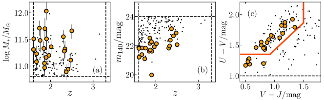
Figure 1.— Physical properties of the initial photometric sample galaxies (dots) and final 24 galaxies (orange circles). The criteria used for the initial photometric selection are shown with dashed lines. (a) Stellar-mass distribution as a function of redshift. (b) The F140W magnitude distribution as a function of redshift. (c) The UVJ-color diagram. Our sample consists of both quenched (left-top region bounded by solid lines) and quenching (those $U-V>1$ but outside the boundary) galaxies.

2.2. HST Grism Spectrum

In M1149, the grism data were taken through GLASS (Schmidt et al., 2014; Treu et al., 2015). GLASS is a spectroscopic survey with HST/WFC3 G102 and G141 grisms (10 and 4 orbits, respectively). In addition, we supplement with the follow-up HST-GO/DDT campaign (Proposal ID 14041, PI: P. Kelly) of the multiply imaged supernova, SN Refsdal (Kelly et al., 2015, 2016), which adds another 30 orbits of G141 data to the original GLASS observation.

In GDN/GDS, we retrieve the public data through MAST. In addition to the 3DHST data (van Dokkum et al., 2013b; Momcheva et al., 2016) that cover entire CANDELS’s GDN/GDS fields, we add those taken in FIGS (13779; PI: S. Malhotra Pirzkal et al., 2017), CLEAR (14227; PI: C. Papovich, also Estrada-Carpenter et al., 2018), and other follow-ups (12099&12461; PI: A. Riess, 12190; A. Koekemoer, 13420; PI: G. Barro, 13871; PI: P. Oesch).

We extract 1D spectra from all fields in a consistent way, by using the latest version of Grizli (Brammer, 2018). During the extraction, the code automatically models neighboring objects, which are flagged in pre-provided SExtractor segmentation maps, and produces clean spectra for a target galaxy. The clean, optimal extracted spectra from each position angle (PA) is then stacked in a refined wavelength grid of $45$ Å/ pixel. The pixel scale is slightly finer than the Nyquist sampling of G141 grism, since we have many sampling over different orbits, each of which slightly shifts in the dispersion direction. Each spectrum is convolved with the image of the source to match the morphological difference in different PAs.

For the aperture correction of broadband photometry, we match the pseudo-broadband flux extracted from grism spectra by convolving with the corresponding filters (F140W/F105W) to the observed broadband flux (Section 3.2).

In addition to the random uncertainty in flux, we also estimate the uncertainty associated with the stacking of different PAs by following Onodera et al. (2015), and we integrate this to the random noise in quadrature for conservative estimates. The uncertainty accounts of $\sim 20\%$ of the random uncertainty. Signal-to-noise rations (S/Ns) of the final 1D spectrum range up to $\sim 50$. Median values of each spectral element are ${\rm S/N}\sim 18$ at $4200$–$5000$ Å and $\sim 4$ at $3400$–$3800$ Å (Table Appendix C: Simulation with Realistic SFHs).

2.3. Additional Photometric Data

In addition to photometric fluxes collected in 3DHST, we add WFC3/UVIS photometry. The rest frame UV coverage is important to constrain SEDs with/without the UV upturn, which depends on metallicity (e.g., Yi et al., 1997; Treu et al., 2005b). We use WFC3/UVIS images from HDUV legacy survey (Oesch et al., 2018), that cover parts of GDN/GDS fields with F275W and F336W filters. The UVIS images in GDS consist of the previous data taken in the UDF by the UVUDF team (Teplitz et al., 2013). We run SExtractor on the public imaging data to conduct photometry and use the flux measured in a fixed aperture of 0.​″72 diameter.

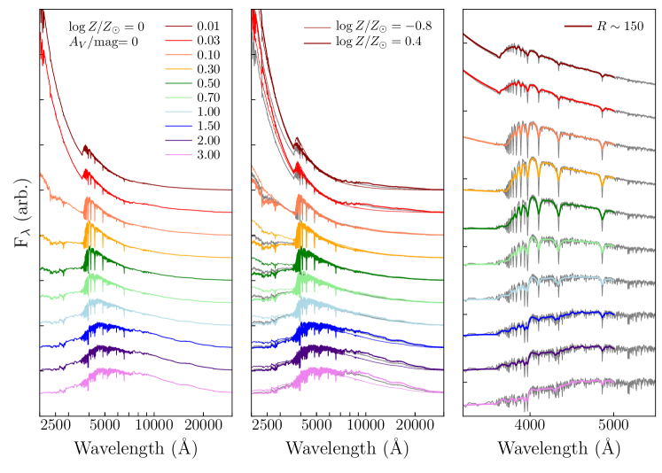
Figure 2.— Left: Original spectral templates used in fitting. Only those with $\log Z_{*}/Z_{\odot}=0$ without dust attenuation ($A_{V}=0$) are shown here, with arbitral shifts in flux. Left: Same as left panel (gray solid lines) but also showing templates with different metallicities for comparison (thin lines for $\log Z_{*}/Z_{\odot}=-0.8$; thick lines for $\log Z_{*}/Z_{\odot}=0.4$). Templates are normalized at $5000$ Å. Right: Same as left panel (gray solid lines) but also showing spectra that are degraded to match the observation, that accounts for the G102/G141 resolutions and source morphology ($R\sim 150$; colored lines).

3. Spectrophotometric SED fitting

3.1. Basic Templates

Our SED fitting method (Grism SED Fitter, or gsf; Morishita, in prep.) is based on the canonical template fitting, where the best-fit parameters are determined by minimizing the residuals of observed and model SEDs. One major difference from most of other works is the way we construct the model templates. SED templates are often constructed with a functional form for SFHs, such as the exponential declining model, $\psi\propto A\exp[-(t-T_{0})/\tau]$, where $A$, $T_{0}$, and $\tau$ are free parameters. However, it is known that such a simplification may not represent real galaxy SFHs by observations (e.g., Pacifici et al., 2016; Iyer & Gawiser, 2017) and simulations (e.g., Diemer et al., 2017). As such, we here avoid any functional forms and adopt an alternative method to generate model templates. The core of the method is to find the best combination of amplitudes, $\{a_{i}\}$, for a set of composite stellar population (CSP) templates of different ages, $\{t_{i}\}$, that matches the data, as previously performed by Morishita et al. (2018). This type of SED modeling has been used in previous studies (Heavens et al., 2004; Cid Fernandes et al., 2005; Panter et al., 2007; Tojeiro et al., 2007; Kelson et al., 2014; Dressler et al., 2018), some of which demonstrated its strength and validity with intensive simulation tests.

To generate the template with different parameters, we use the flexible stellar population synthesis code (FSPS; Conroy et al., 2009; Conroy & Gunn, 2010; Foreman-Mackey et al., 2014) to generate $i$th templates with ages of $t_{i}$, based on MIST isochrones (Choi et al., 2016) and the MILES stellar library. As found by Morishita et al. (2018), different isochrones may return different results, in addition to a systematic difference in assumed metallicities.

We set the number of age “pixels” to 10, with [0.01, 0.03, 0.1, 0.3, 0.5, 0.7, 1.0, 1.5, 2.0, 3.0] Gyr (Figure 2), doubling the number from those adopted in Morishita et al. (2018). While we set the equal width of template in log normal space ($\sim 0.5$) following previous studies (e.g., Cid Fernandes et al., 2005), we added extra bins at intermediate age, where most of our galaxies are located, to increase the flexibility of SFHs.

The template is generated by assuming a short constant star formation rate within each bin width ($\sim 30$ Myr), rather than a simple stellar population (SSP). The reason we do not adopt the SSP model is that, while it is simple, it is unrealistic for real galaxies. Changing the width of constant star formation in each bin would result in a minor but systematic shift in reconstructed SFHs. The uncertainty in bin width is considered in calculation of parameters (e.g., age), by randomly fluctuating values within the width.

We also set metallicity of each age pixel as a free parameter in a range of $\log Z_{*}/Z_{\odot}\in[-0.8:0.6]$, as opposed to one global value in Morishita et al. (2018). While determination of metallicity at each age pixel (i.e. metallicity histories of individual galaxies) is more challenging (see Appendix A), this gives extra flexibility in fitting templates, and allows reasonable estimate of uncertainty in SFHs (Section 5.3).

It is noted that metallicity sensitive lines (such as Fe and Mg) are not measured at our spectral resolution. Our method rather relies on the entire spectral shape with grism spectra and wide broadband photometry, that spans from NUV, optical (that are sensitive to age), to NIR (to metallicity) wavelength range (see Figure 2).

Templates generated with MIST are uniformly set to the solar-scaled abundance (Asplund et al. 2009; i.e. $[\alpha/{\rm Fe}]=0$). It is noted that galaxies at high $z$ may have an $\alpha$-enhanced chemical composition (e.g., Onodera et al., 2015; Kriek et al., 2016), as found in local early-type galaxies (e.g., Thomas et al., 2005; Walcher et al., 2015). In fact, enhancement of $\alpha$-element has a similar effect as that of iron in UV and NIR continuum slopes (e.g., Vazdekis et al., 2015), while our low-resolution spectra cannot capture a detailed difference in each absorption line (i.e. Lick indices), and both abundances are degenerated in our total metallicity measurement, $\log Z_{*}/Z_{\odot}$. As such, our total metallicity should remain similar to those with, e.g., $\alpha$-enhanced templates (see also Walcher et al., 2009).

We assume a Salpeter (1955) initial mass function and Calzetti et al. (2000) dust law, where the dust attenuation, $A_{V}$, is a global parameter that is applied to all age templates equally. Redshift is set as a free parameter at this step but within the $3\,\sigma$ range estimated in the previous step. In sum, the fits have $10\times 2+1+1=22$ free parameters.

The degree of freedom of our fitting is worth noting. The number of spectral data points for each of our galaxies is $>200$ (with $\sim 16$ for broadband photometric data points), where the spectral element is set to $45$ Å in this study. Considering the correlation due to morphology (which is $\sim 104$ Å for the mean size of our galaxies, $r\sim 0.3\arcsec$), and the large number of parameters, our spectra still have $\sim 100$ independent data points.

Our updated method here has a few advantages over Morishita et al. (2018). First, it is more flexible than an a priori assumption of the SFH, and robust to systematic bias in derived parameters (e.g., Wuyts et al., 2012). Second, it is flexible to a complex shape of SFHs, such as those with multiple bursts and sudden declines (e.g., Boquien et al., 2014). A SFH with multiple peaks cannot be reproduced by the exponential declining model (see Section 4). Third, it is flexible to the metallicity evolution. Methods with functional forms often have a fixed metallicity over the entire history. In our method, each template at a different age has a flexibility in metallicity as a free parameter that also provides metallicity enrichment histories, though the uncertainty in each age is typically large for most of our data sets in this study (Appendix A).

3.2. SED parameter exploration

The combination of templates is controlled by changing each amplitude, $a_{i}$, as free parameters during the fit. A challenging part is the large number of parameters (over a dozen, compared to $\,\hbox to0.0pt{\lower 3.5pt\hbox{$\mathchar 0\relax\sim$}\hss}\raise 1.0pt\hbox{$<$}\,5$ parameters with functional SFHs), which could be trapped in local minima. To sufficiently, yet efficiently, explore the parameter space, we adopt the Markov chain Monte Carlo (MCMC) method.

The fitting process of gsf is twofold: (1) initial redshift determination based on visual inspection of absorption lines, and (2) MCMC realization to estimate the probability distribution for all parameters.

First, gsf determines the redshift by fitting the model templates to the observed grism spectra. At this point, it only generates model templates in the wavelength range of grism spectra, to minimize the computational cost. The templates are convolved to the resolution of the spectra with a Moffat function derived from the observed source morphology for spectra. It searches the best-fit redshift by minimizing $\chi^{2}$, as well as visual inspection, to avoid catastrophic errors. During the visual inspection, we rely on the major absorption lines in the observed range (i.e. H$\delta$, H$\gamma$, H$\beta$), and thus those without clear absorption features (i.e. low S/N) are discarded here. At this step, gsf also determines the scale of the G102/G141 spectra so that each matches to the broadband photometry in F105W and F140W at a given template. The added scale for our sample is small ($\,\hbox to0.0pt{\lower 3.5pt\hbox{$\mathchar 0\relax\sim$}\hss}\raise 1.0pt\hbox{$<$}\,10\%$) thanks to the accurate sky-background estimation in Grizli.

Then, gsf generates a template library at the redshift determined in the previous step and fits SEDs at the entire wavelength range. gsf fits the observed spectra and broadband photometry simultaneously by using emcee (Foreman-Mackey et al., 2013) as in Morishita et al. (2018). Redshift is also explored at this step by shifting and refining the template wavelength grid at a proposed redshift of each MCMC step. Emission lines, if detected, are masked during the fit. Those lines are modeled with a gaussian function after subtracting the best-fit SED template to estimate the line flux and equivalent width (EW; Section 4.2).

We set the number of walkers to 100 and the number of realization, $N_{\rm mc}$, to $10^{5}$. We adopt an uniform prior for each parameter over the parameter ranges, $a_{i}\in[0:1000]$, $\log Z_{*}/Z_{\odot}\in[-0.8:0.6]$, and $A_{V}/$mag$\in[0:4]$. The effect by the amplitude prior (i.e. SFH; see Figure 12) should be minimal due to the wide constrain range, as seen in the simulation in Appendix A. While some of previous studies set a prior in metallicity histories from the local mass metallicity relation (e.g., Pacifici et al., 2016; Leja et al., 2018) (i.e. increasing metallicity as a function of time), we find that our result reproduces this behavior without such priors. However, the age-metallicity degeneracy could also mimic this trend. Our test with a mock data set (Appendix A) revealed, while the trend is fairly reproduced, nonnegligible scatters in derived metallicity at each age pixel, and that metallicity histories of individual galaxies remain less promising (see also below).

During the fit, we let emcee run with the parallel tempering sampling, with $n_{\rm temp}=5$. With this, emcee samples the parameter spaces but with $n_{\rm temp}$ samplers in parallel. Each sampler has a different value for the temperature parameter in a Metropolis–Hastings step, i.e. a higher temperature makes a larger step in a parameter space. With this, the sampler suffers less from the local minima. We note, however, that a sufficient number of MCMC realizations (which is inferred from a simulation test for our case) is necessary to estimate reliable uncertainties. Otherwise, derived uncertainties would become inappropriately small, with possible biases in the best-fit values (see Cid Fernandes, 2018).

The first half realization of the sampled chain is discarded to avoid biased results from initial input values. We take the 50th and 16th/84th percentiles of marginalized distributions as the best-fit and uncertainty range.

To check the reliability of SED parameters and reconstructed histories, we conducted a simulation test with mock data set (Appendix A). From the test, we found that the scatter in the reproduced amplitude and metallicity at each age bin is $\sim 0.5$ dex and $\sim 0.25$ dex, respectively. To account for this, we add the estimated scatter to the reconstructed star formation and metallicity histories, which are also propagated to other SED parameters (Section 4.3).

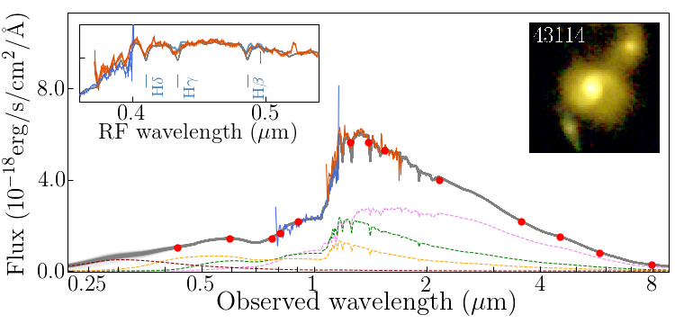
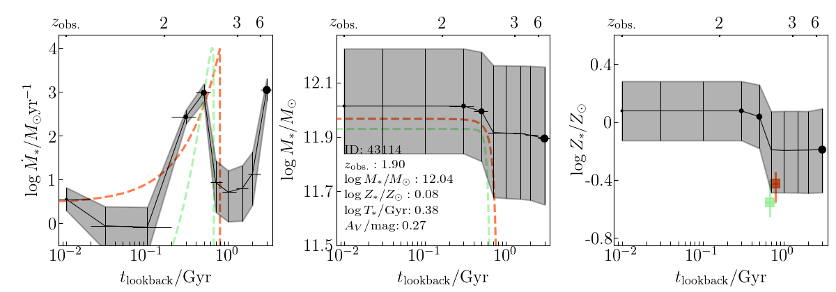
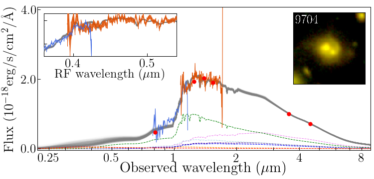
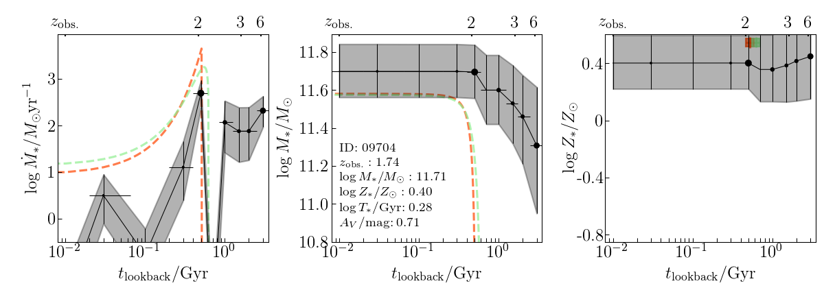
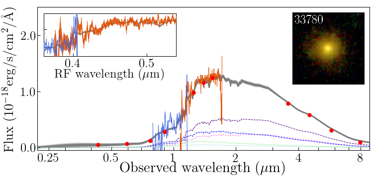
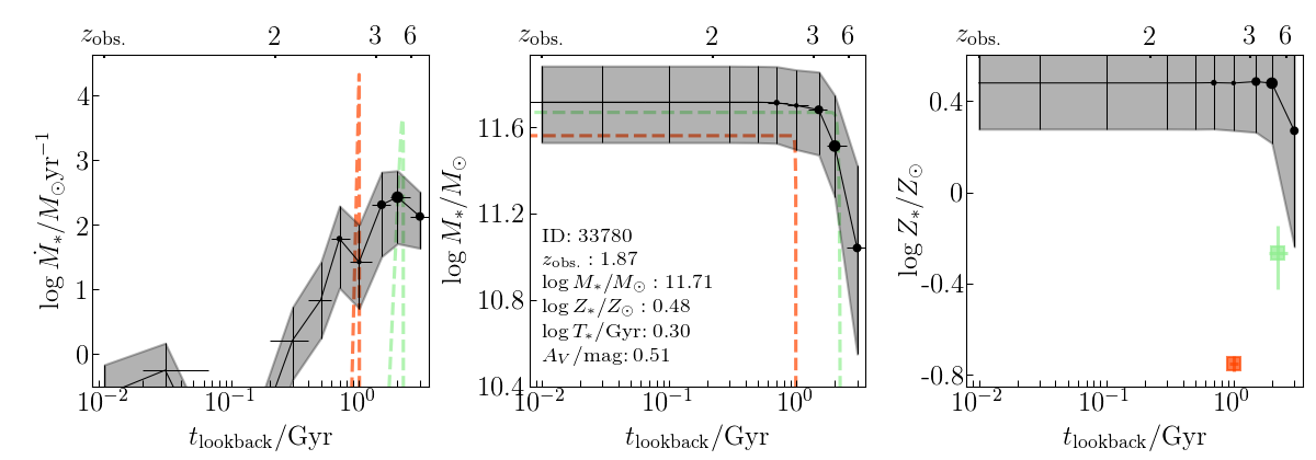
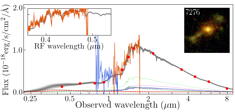
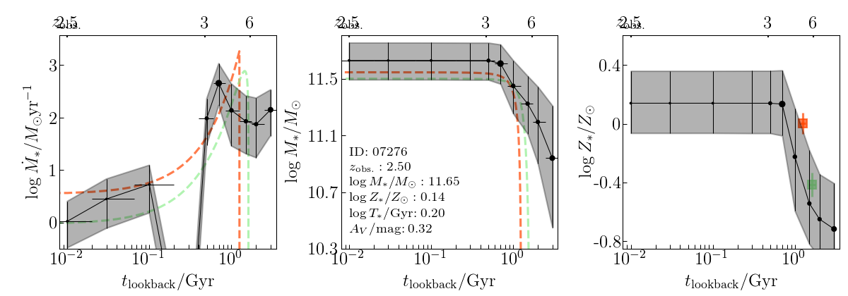
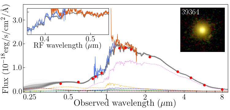
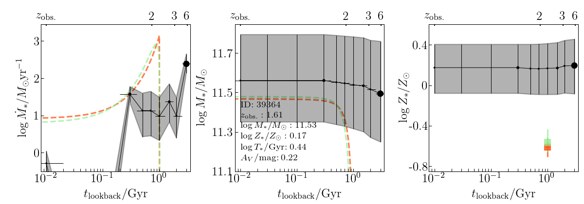
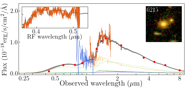
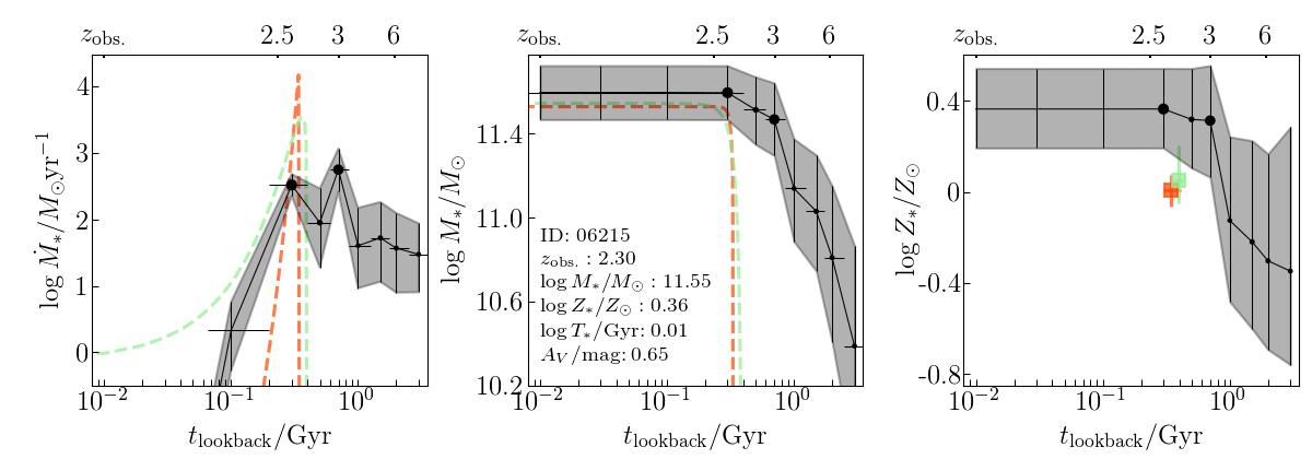
Figure 3.— Results of SED fitting for the final 24 galaxies sorted in order of stellar mass. First column: observed spectra (blue and red lines with error bars for G102 and G141) and photometric data points (red circles with black error bars). The best-fit templates of each age bin (dashed lines, colored as in Figure 2) and the sum (gray dashed lines) are shown. Different total templates randomly reproduced from the MCMC chain are also shown. Pseudo-color stamps (F160/125/814W for R/G/B; $4.8\times 4.8$ arcsec${}^{2}$) are shown. Emission lines, when detected, are shown with fitted Gaussian curves in the inset (blues solid lines). Second column: reconstructed star formation histories, with the 50th (black circles) and 16th/84th percentile ranges (gray hatched region) shown. The size of the symbols at each age bin (black circles) represents the amplitude. The best-fit SFHs with functional forms ($\tau$ and delayed-$\tau$ models) are also shown for comparison (red and green dashed lines). Third column: same as second column, but for stellar-mass accumulation histories. Fourth column: same as second column, but for mass-weighted stellar metallicity. The best-fit metallicities derived by the two functional models are shown at the best-fit age (red/green squares with error bars).

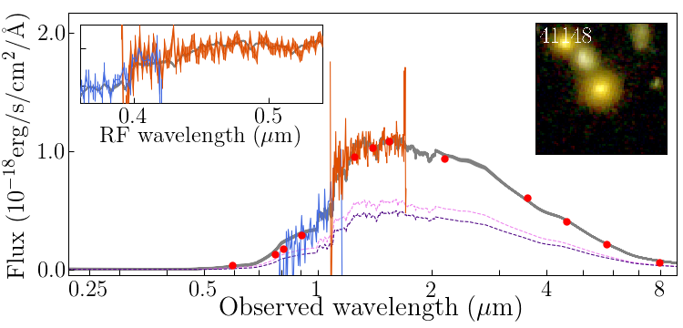
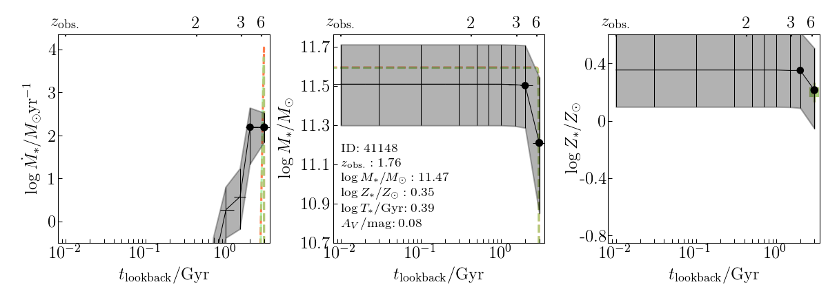
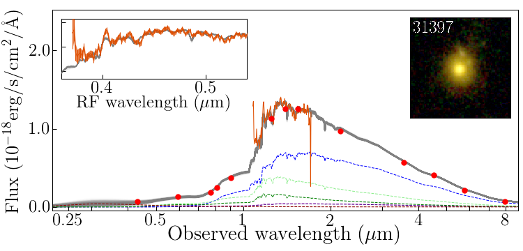
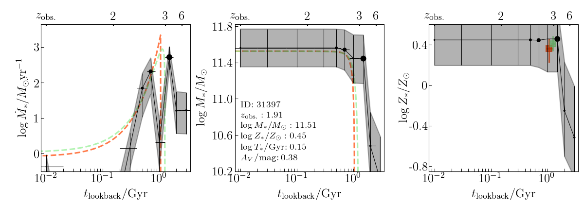
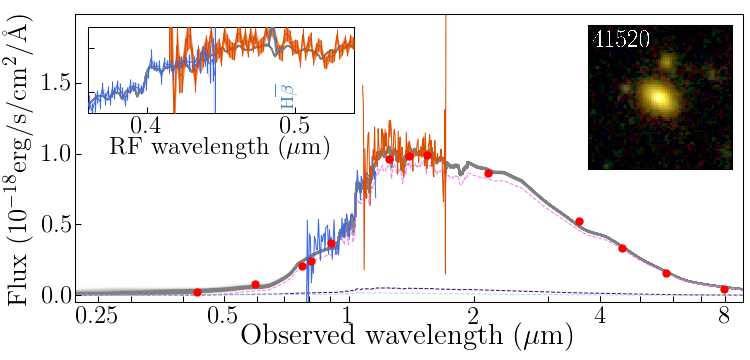
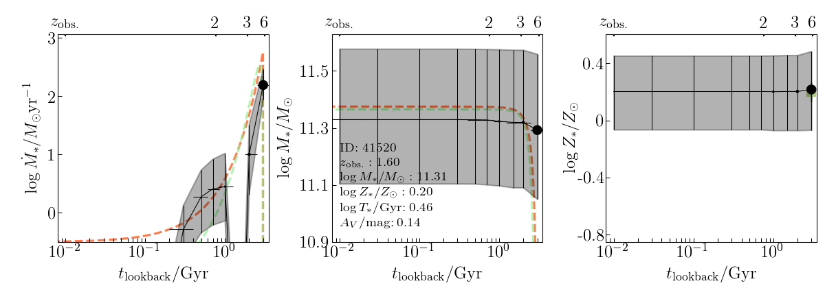
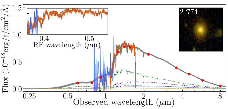
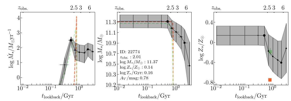
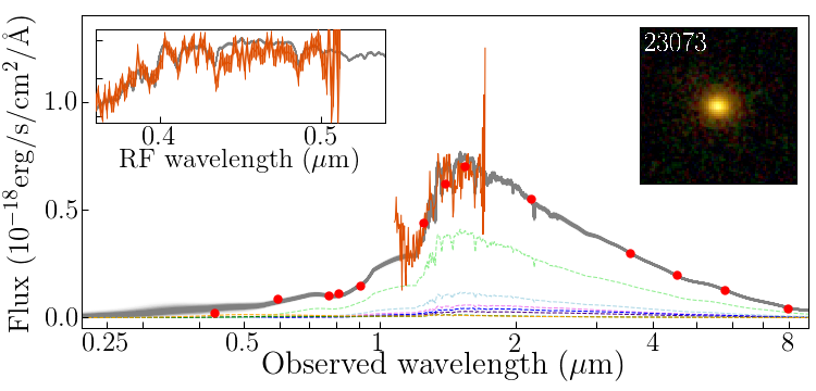
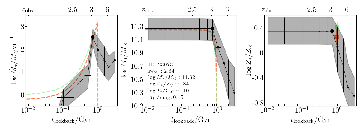
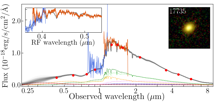
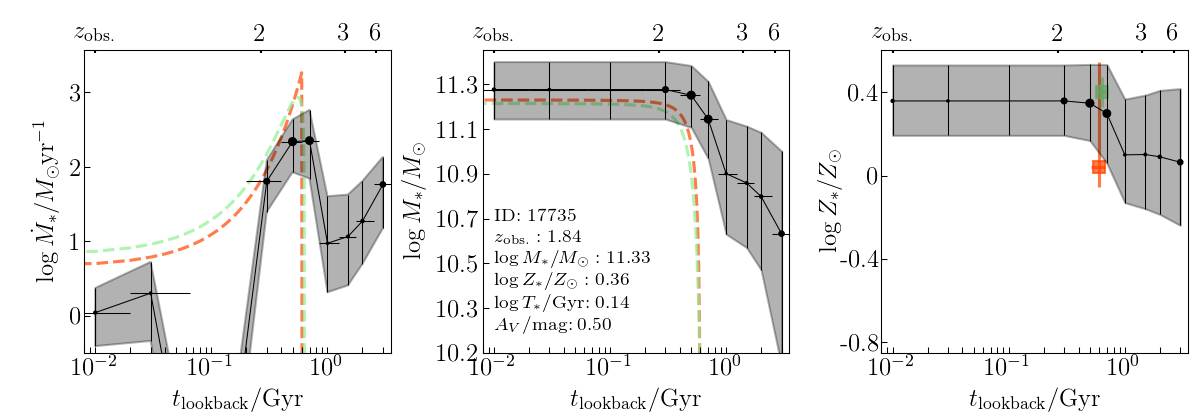
Figure 3.— Continued.

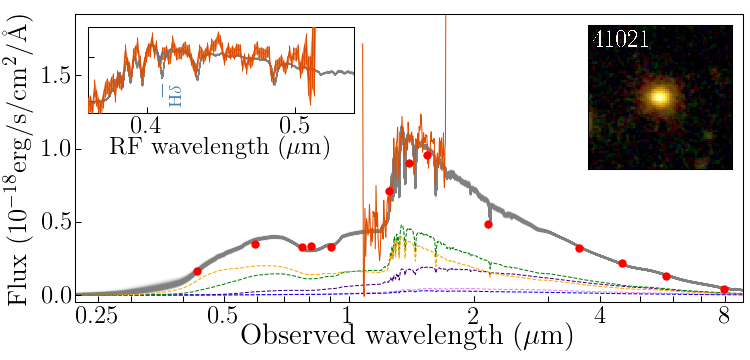
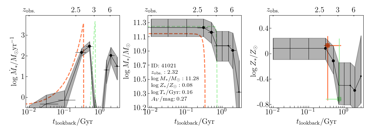
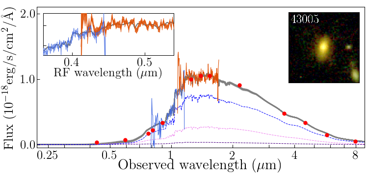
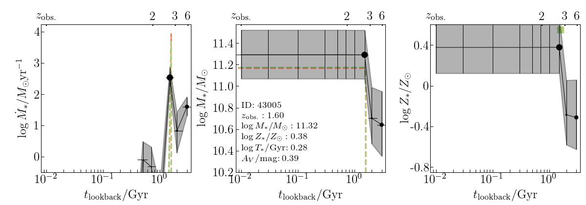
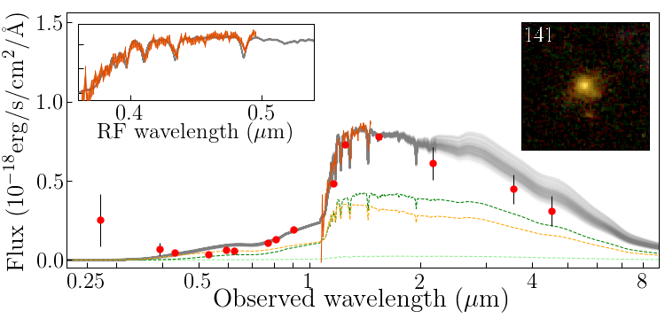
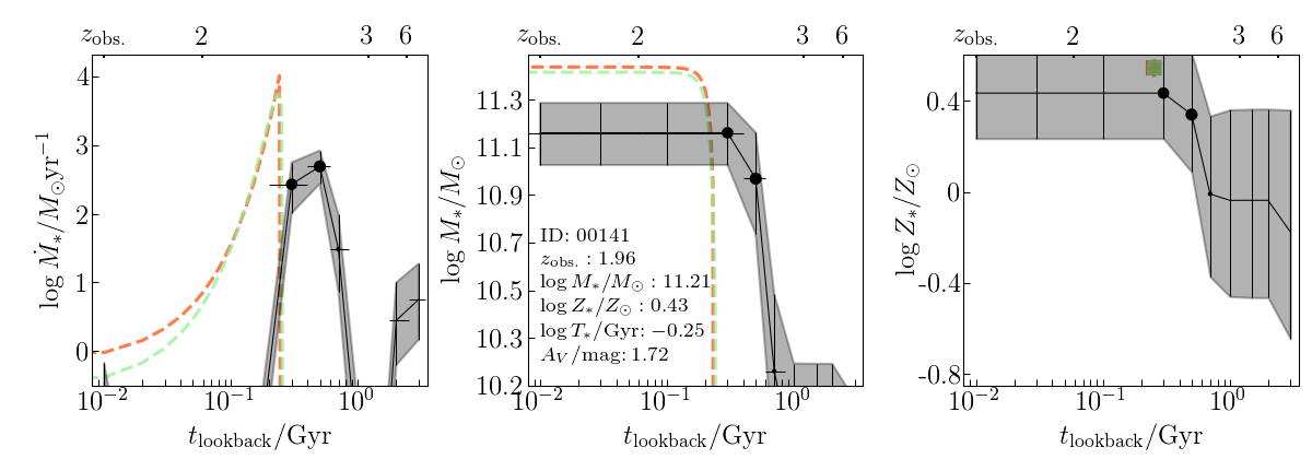
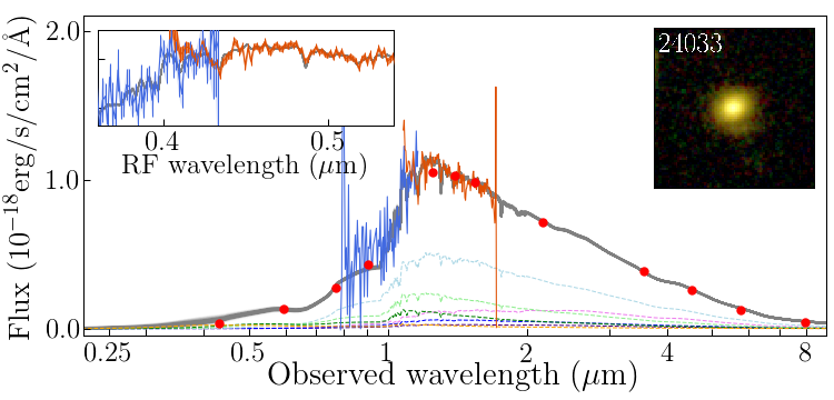
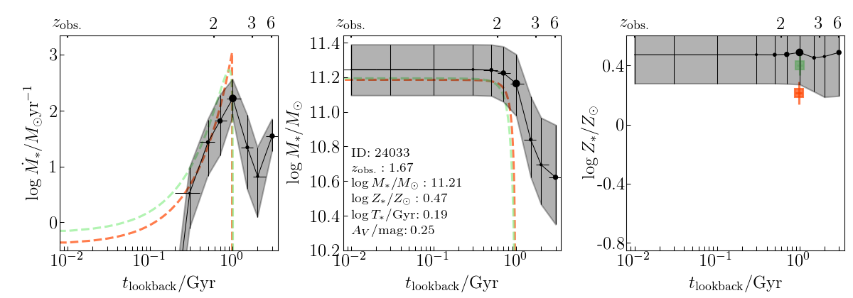
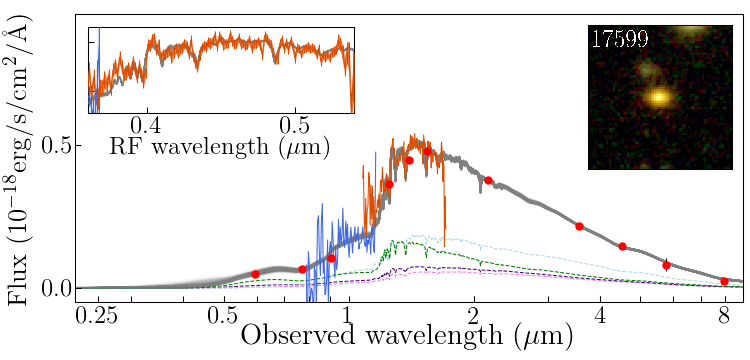
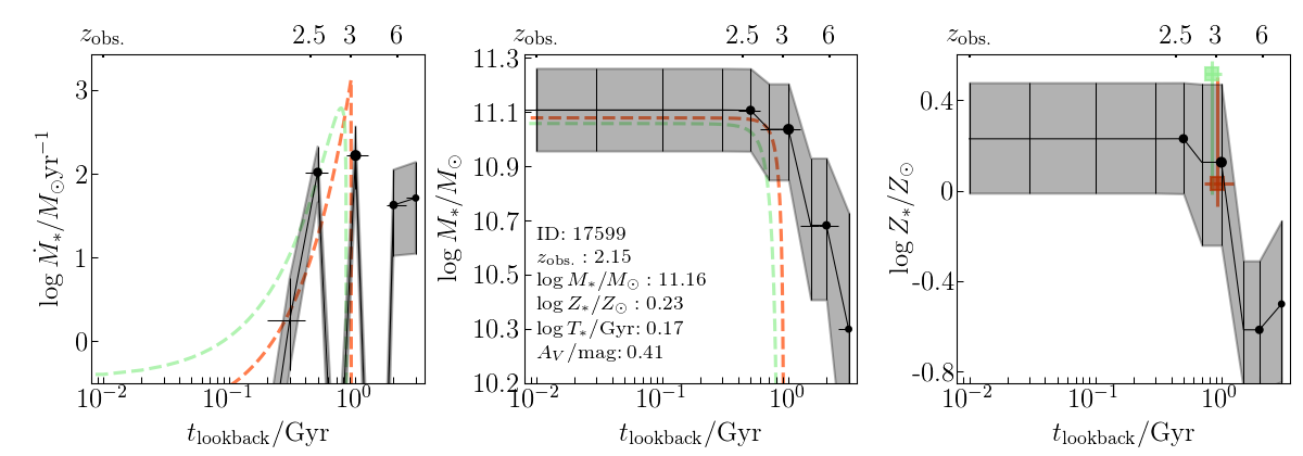
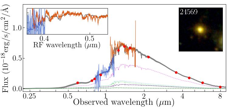
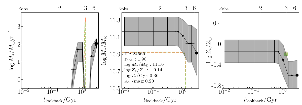
Figure 3.— Continued.

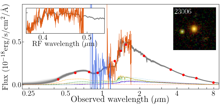
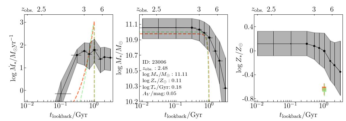
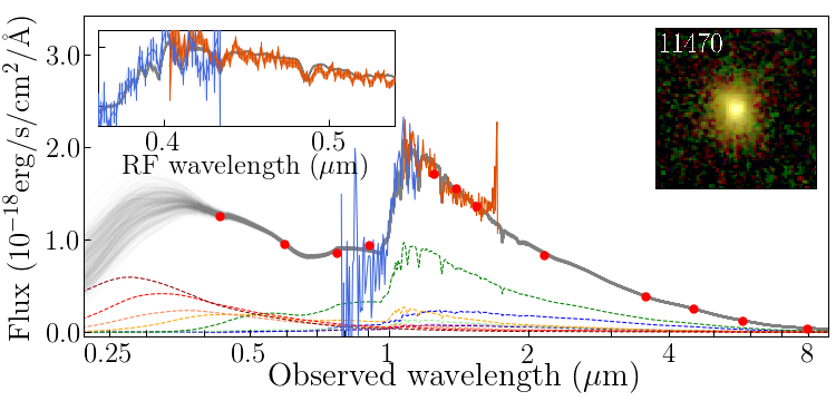
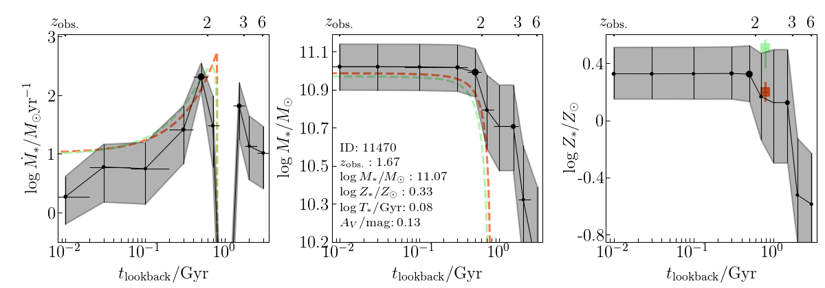
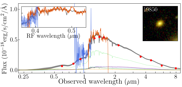
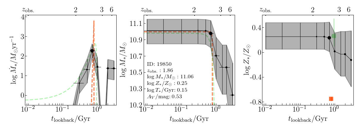
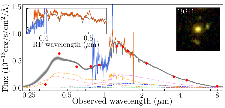
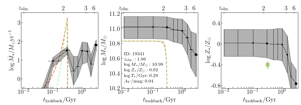
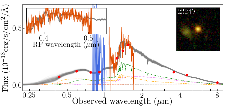
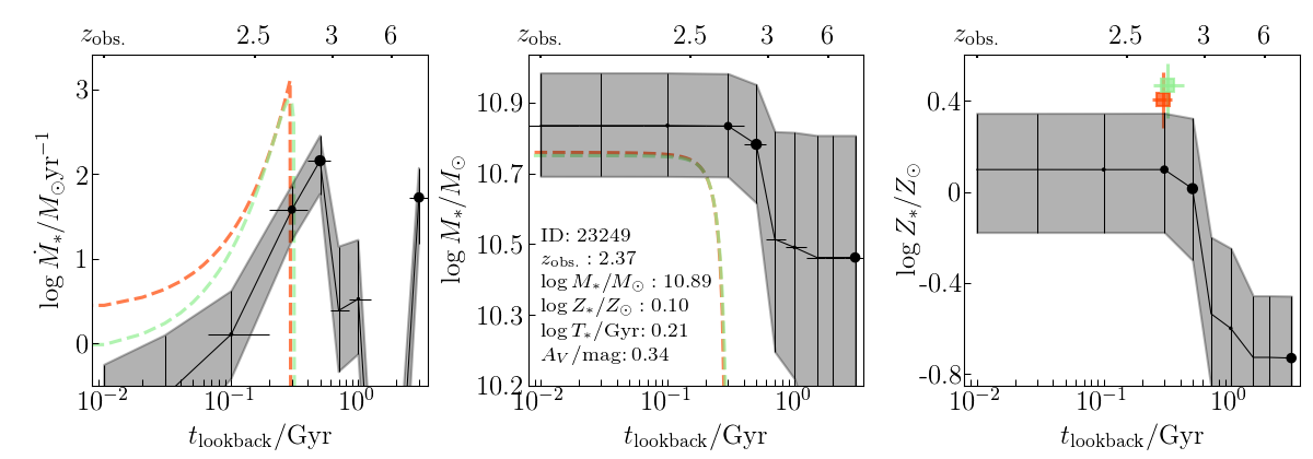
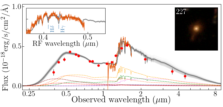
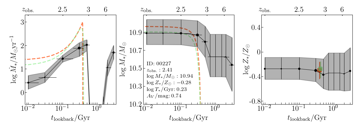
Figure 3.— Continued.

4. Results

4.1. Twenty-Four Galaxies as the Final Sample

In Figure 1, we summarize basic parameters of final sample galaxies. The final sample consists of 2, 12, and 10 galaxies from M1149, GDN, and GDS, after the rest of initial samples are visually discarded because of poor redshift fitting quality (Section 3.2). Due to the partial coverage of the grism observations, and also random contamination from neighboring galaxies, our samples have nonuniform exposure time in the grism observation and signal to noise ratio (S/N; Table Appendix C: Simulation with Realistic SFHs). The two galaxies in M1149 are those previously reported by Morishita et al. (2018).

In panels (a) and (b) of Figure 1, we plot the distribution of our sample galaxies in redshift–stellar mass/F140W–magnitude spaces, respectively. Due to the increasing sensitivity of G141 grism with wavelength, galaxies at higher redshift are fainter in F140W than those at lower redshift. In (c), we show the UVJ color-color diagram for diagnosing galaxy quiescence (e.g., Williams et al., 2009). While most of the sample locates within the passive category, there are six galaxies that fall below the passive/star forming boundary in $U-V$. These galaxies are in transition between star forming ($U-V\,\hbox to0.0pt{\lower 3.5pt\hbox{$\mathchar 0\relax\sim$}\hss}\raise 1.0pt\hbox{$<$}\,1$) and passive ($\,\hbox to0.0pt{\lower 3.5pt\hbox{$\mathchar 0\relax\sim$}\hss}\raise 1.0pt\hbox{$>$}\,1.4$), akin to the green valley (or “quenching”) galaxies in the local universe (Kauffmann et al., 2003; Schawinski et al., 2014).

The characteristic age, which is about the time since a system reached its half-mass, of each galaxy represents the mass-weighted value from the reconstructed SFH,

$$T_{*}=\sum_{i}t_{i}a_{i}\Psi_{i}/\sum_{i}a_{i}\Psi_{i}$$ (1)

where $t_{i}$ is the median age, $a_{i}$ best-fit amplitude, and $\Psi_{i}$ mass-to-light ratio of $i$-th template. An estimated error for each amplitude from the simulation test (Appendix A) is added in quadrature. The typical error in mass-weighted age is $\sim 0.2$ dex.

The derived parameters are summarized in Table Appendix C: Simulation with Realistic SFHs. It is noted that estimated errors in stellar mass are larger ($\sim 0.2$ dex) than those listed in original catalogs ($\,\hbox to0.0pt{\lower 3.5pt\hbox{$\mathchar 0\relax\sim$}\hss}\raise 1.0pt\hbox{$<$}\,0.1$ dex; Skelton et al., 2014). This is due to the fact that our fitting accounts for an additional uncertainty originated in the flexibility of SFHs. While one can implement this by e.g., repeating a SED fitting analysis with different SFHs (Wuyts et al., 2012; Morishita et al., 2015), the stellar mass measurement in the original catalog (as well as many others) is based on one functional form for SFHs, and thus the quoted errors are solely from photometric error and redshift (see also Appendix B).

4.2. Diagnostics from the SED shape

In the left panels of Figure 3, we show SEDs of the sample galaxies with the best-fit templates. Our galaxies are well characterized with $k+a$ (Dressler & Gunn, 1983) and quiescent spectra, as is expected from the sample selection and redshift range. Deep spectra successfully capture spectral features of these types of galaxies, such as absorption lines and $4000\,{\rm\AA}$/Balmer break. The wide broadband coverage well captures spectral features, such as a blue UV slope from a young population ($\sim 1$ Gyr) and near-IR excess from an old population ($\,\hbox to0.0pt{\lower 3.5pt\hbox{$\mathchar 0\relax\sim$}\hss}\raise 1.0pt\hbox{$>$}\,2$ Gyr), that is consistent with the derived mass-weighted age ($T_{*}$; see Table Appendix C: Simulation with Realistic SFHs).

Six galaxies have moderately detected ($\sim 1.5\sigma$) weak emission lines, such as [O ii], H$\delta$, H$\gamma$, and H$\beta$, which is a signature of ongoing star formation. We first fit each emission line with a Gaussian after subtracting the best-fit spectrum. The EW is then measured with the total flux from the Gaussian fit and the best-fit template as a continuum. For [O ii] line, we use Eq.3 in Kennicutt (1998) to estimate the star formation rates. For H$\beta$ line, we use assume a recombination coefficient in the Case B (Osterbrock, 1989) and then Eq.2 in Kennicutt (1998). These weak emission lines indicate specific star formation rate (SFR/$M_{*}$) of $\,\hbox to0.0pt{\lower 3.5pt\hbox{$\mathchar 0\relax\sim$}\hss}\raise 1.0pt\hbox{$<$}\,10^{-10}$ yr${}^{-1}$. While the detection is tentative, the low level of star formation activity is also observed in previous findings (e.g., Belli et al., 2017), possibly providing more detailed pictures of quenching mechanisms (Section 5). Two of the emission detected galaxies (IDs 19341 and 19850) have strong [O iii] lines ($4959+5007\,{\rm\AA}$) with a relatively weak H$\beta$ line, suggesting existence of active galactic nuclei (AGNs). While H$\alpha$ and $[\textrm{N}~{}\textsc{ii}]$ are beyond our wavelength coverage, the line ratio of H$\beta$ and $[\textrm{O}~{}\textsc{iii}]$ lines ($\log\textrm{H}\textsc{$\beta$}/[\textrm{O}~{}\textsc{iii}]\ =0.15\pm 0.03$ and $0.13\pm 0.05$) implies that these galaxies as AGNs in the mass-excitation diagram (Juneau et al., 2014).

On the other hand, we find six galaxies that consist of very old populations with mass-weighted ages $\,\hbox to0.0pt{\lower 3.5pt\hbox{$\mathchar 0\relax\sim$}\hss}\raise 1.0pt\hbox{$>$}\,2$ Gyr, and dominate high-mass end among our sample. While such massive galaxies are rare ($n\sim 3\times 10^{-5}$ Mpc${}^{-3}$; Muzzin et al., 2013; Tomczak et al., 2014), it is also true that some of ancient galaxies, that formed a long time ago, have more chance to experience ex-situ processes, e.g., merger and gas accretion, especially at this high redshift. Such ancient galaxies would be smuggled into younger population and become indistinguishable when seen with e.g., light-weighted age. Our reconstructed SFHs have ability to investigate this.

4.3. SFHs

In the right three columns of Figure 3, we show the reconstructed SFHs, mass accumulation histories, and metallicity enrichment histories for our sample galaxies. We reconstruct SFRs in each time bin by dividing the amount of stellar mass formed (including the lost mass by the time of observation) by the bin length. Thus, SFRs at each bin represent its average values over the time ($\sim 30$ Myr for the youngest template to $\sim 1$ Gyr for the oldest one). It is also noted that the derived SFR cannot distinguish between to in-situ (stars formed in the system) or ex situ (those obtained via mergers).

Some galaxies are worth highlighting. For example, ID 43114, the most massive galaxy among our sample ($\log M_{*}/M_{\odot}\sim 12$; also van Dokkum et al. 2010 and Ferreras et al. 2012), formed about 50% of the final mass already at $z\,\hbox to0.0pt{\lower 3.5pt\hbox{$\mathchar 0\relax\sim$}\hss}\raise 1.0pt\hbox{$>$}\,5$ ($\sim 2$ Gyr ago). The galaxy was at low star formation activity for $\sim 1.5$ Gyr, and then started active star formation ($\sim 1000\,M_{\odot}$/yr) at $z\sim 2.5$, $\sim 300$ Myr ago. The significant star formation is comparably high as those of sub-millimeter galaxies at this redshift (Younger et al., 2007; Tacconi et al., 2008). In fact, its morphology shows a tidal feature with two close objects at the outer part, suggesting a recent (major) merger. Its star formation activity seen in the reconstructed SFH is consistent with a typical merger time scale at this redshift (Lotz et al., 2011; Snyder et al., 2017). Interestingly, the dust attenuation of this galaxy is relatively low ($A_{V}\sim 0.3$ mag) compared typical sub-millimeter galaxies and starburst galaxies at this redshift ($A_{V}>3$ mag; Riechers et al., 2013; Toft et al., 2014), suggesting post processes might have cleared a large amount of dust.

Other galaxies with clearly disturbed morphology (e.g., IDs 09701 and 00141) also show recent intense star formation at $\,\hbox to0.0pt{\lower 3.5pt\hbox{$\mathchar 0\relax\sim$}\hss}\raise 1.0pt\hbox{$<$}\,1$ Gyr before $t_{\rm obs}$, that may provide independent constraint in merger time scale and induced star formation activity from follow-up kinematical studies.

Interestingly, many of our galaxies show extended star formation activity to $\sim 0.3$ Gyr before their observed redshifts. This differs from previous understanding of massive early-type galaxies, whose star formation activity was believed to decline rapidly or truncated after forming the bulk of stars in a very short time. While our sample size here is too small to generalize this (see also Ferreras et al., 2019), and is also possibly biased to a high-surface density population, it is curious to investigate how previously adopted functional form SFHs behave to such extended feature, as well as other features like dual-peak SFHs.

We repeat the same analysis but with functional forms of SFHs to compare with our SFHs. In Figure 3, we show the best-fit SFHs obtained with a functional form for the SFH, $\tau$-model with $\propto A\exp[-(t-t_{0})/\tau]$. In addition to $\tau$ and $t_{0}$, we allocate one parameter for metallicity, and one for dust attenuation. In most cases, it is clear that SFHs derived from gsf cannon be reproduced by the $\tau$-model. For example, the $\tau$-model cannot capture the dual peaks observed in some of our galaxies (e.g., ID43114). The $\tau$-model also fails to capture extended star formation, both at young and old age sides. This is due to the fact that the functional SFH is light-weighted, where the best-fit parameters are more sensitive to differential amounts of light. Such qualitative discrepancy in fact results in quantitative discrepancy in the best-fit parameters, with $\chi^{2}/\nu$ systematically larger than gsf (see also Carnall et al. 2018, who argue limitation by a functionally defined SFH). Appendix B summarize the comparison of the $\tau$-model, and also results with the delayed $\tau$-model.

Metallicity histories shown in Figure 3 represent mass-weighted accumulated metallicity,

$$Z_{j}=\sum_{i}^{i\leq j}Z_{i}a_{i}\Psi_{i}/\sum_{i}^{i\leq j}a_{i}\Psi_{i},$$ (2)

where $i$ covers older age pixels than $j$. Individual metallicity values at each age pixel often suffer from large uncertainty ($\sim 0.25$ dex; Appendix A), while this is partially attributed to small amount of light in those age pixels (i.e. small $a_{i}$). We therefore avoid discussing metallicity enrichment histories of individual galaxies, but rather focus on (more robust) total metallicity in this study (Section 5.3). It is noted, however, that having parameters for metallicity at each age bin allows flexibility in fitting, and more reasonable estimate (i.e. larger error bars) in SFHs and SED parameters.

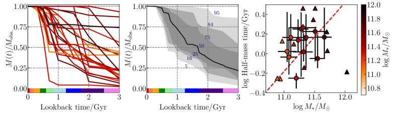
Figure 7.— SFHs as a function of lookback time from the observed redshift. Left: cumulative stellar mass evolution of individual galaxies. Color corresponds to the final stellar mass. Ages that correspond to the SED templates are indicated with color bars at the bottom (colored as in Figure 2). Middle: summary of individual cumulative stellar mass evolution, where contour boundaries and line correspond to the 5/16/25/75/84/95th percentiles and median. Right: half-mass time (lookback time from $t_{\rm obs}$; $t_{50}$ in the main text) as a function of observed stellar mass. Those with lower limits are shown with triangles. Symbol color corresponds to the final stellar mass. A positive correlation, $\log t_{50}$ /Gyr $\propto 0.5\log M_{*}/M_{\odot}$, is seen (red dashed line; i.e. downsizing).

5. Discussion

5.1. Time scale of star formation

In Figure 7, we summarize the mass accumulation histories as a function of lookback time from the observed redshift. Most of our sample galaxies formed $>50\%$ of their extant mass by $\sim 1.5$ Gyr prior to the observation ($z\sim 2.5$ to 5, depending on the observed redshift), which is quantitatively consistent with recent studies at similar and higher redshift (Domínguez Sánchez et al., 2016; Schreiber et al., 2018; Estrada-Carpenter et al., 2018; Belli et al., 2019).

We estimate the half-mass time, $t_{50}$ (lookback time from the observed redshift), from individual SFHs in the right panel of Figure 7. $t_{50}$ is estimated in each step of MCMC, and thus its uncertainty represents those in SFHs and also individual age bin widths. For some galaxies, we only estimate the lower limit, as $>50\%$ of stellar mass is in the oldest template. Higher resolution spectra by e.g., JWST are required to reveal ancient histories at a higher time resolution.

Still, we see a trend where more massive galaxies form earlier, known as downsizing (Cowie et al., 1996; Heavens et al., 2004; Treu et al., 2005a), with a linear fit of $\log t_{50}$ / Gyr $\propto 0.5\log M_{*}/M_{\odot}$. The measured standard deviation ($\sim 0.16$ Gyr) is comparable to the redshift range of our galaxies ($\Delta\log T\sim 0.14$ Gyr). The fact that the downsizing trend exists in the early time of the universe provides hints to the galaxy evolution at even earlier epochs, when they were star forming galaxies, and how observed luminous galaxies form (Zitrin et al., 2015; Oesch et al., 2016) in relation to, e.g., their environments (Harikane et al., 2019).

Figure 8.— Stellar mass-metallicity relation of 24 galaxies in this study (circles). The symbols are color-coded by formation redshift, $z_{\rm form}$. Running median ($\sim 0.25$) is shown with 16-84th percentile range (red line with hatched region; $\sigma_{\log Z}\sim 0.15$). Most of our galaxies at $z\sim 2$ already have consistent values to the local metallicity value (gray hatched region represents 16-84th percentile range from Gallazzi et al. 2005, with a calibration shift for $+0.15$ dex; Section 5.2).

5.2. Stellar Mass–Metallicity Relation at $z\sim 2$

The stellar mass-metallicity relation is a key diagnostic of galaxies’ chemical and mass maturation histories. The relation encodes the coevolution of stellar mass and chemical enrichment among galaxies, and provides an independent clue to the past evolution than SFHs. The relation is known to hold from the local universe (Gallazzi et al., 2005; Panter et al., 2008; González Delgado et al., 2014), in a wide range of mass (Kirby et al., 2013), up to $z\sim 1$ (Gallazzi et al., 2014; Choi et al., 2014; Leethochawalit et al., 2018). Beyond the redshift, however, it is still studied with a small sample of galaxies and not clear (Onodera et al., 2012, 2015; Kriek et al., 2016; Morishita et al., 2018). While the relation in gas-phase metallicity at $z\,\hbox to0.0pt{\lower 3.5pt\hbox{$\mathchar 0\relax\sim$}\hss}\raise 1.0pt\hbox{$>$}\,1$ may suggest the relation may remain universal to higher redshift (Tremonti et al., 2004; Mannucci et al., 2010; Kewley & Ellison, 2008; Maiolino et al., 2008; Yabe et al., 2014; Zahid et al., 2014; Onodera et al., 2016; Wang et al., 2017), the observed scatter is still large, due to both a selection bias, different tracer of metallicity, and different physical state of gas phase metallicity (e.g., Andrews & Martini, 2013). We here overview the relation at $z>1.6$ for the first time.

In Figure 8, we show the distribution of our galaxies in the stellar mass-metallicity plane. The metallicity here is a mass-weighted value as for the age (Equation 1). While no significant mass dependency of the metallicity is observed, this is because our galaxies occupy the high-mass end and do not span a wide mass range. In fact, the flattening behavior at a high-mass range is consistent with the relation at lower redshift (Gallazzi et al., 2005, 2014). The observed metallicity is significantly high (median of $\log Z_{*}/Z_{\odot}\sim 0.25$) and tight (scatter of $\sim 0.15$-0.25 dex around the median), which is comparable to the observed scatter in the local relation.

While challenging, it is still of particular interest to compare our metallicity measurement with the local relation. To do this, we need to calibrate the absolute value of metallicity. Although Gallazzi et al. (2005)’s stellar-phase metallicity measurement is based on the total metallicity as in this study (as opposed to an element abundance-based measurement), there is a systematic difference due to the adopted isochrones (MIST versus Padova), each of which has a different definition of solar metallicity ($Z_{\odot}=0.0142$ vs. 0.0190). We correct this by applying a $+0.15$ dex offset to the Gallazzi et al. (2005)’s measurement.

Another systematics is the $\alpha$-abundance of the template. While the templates used in this studies are set to the solar composition (Choi et al., 2016), it is not clear, due to the low-resolution of our spectra, if these metallicity is enhanced by $\alpha$-elements, despite its completely different origin from iron (e.g., Thomas et al., 2005). In fact, Leethochawalit et al. (2018) recently found that $\sim 0.16$ dex decrease in iron abundance of massive galaxies at $z\sim 0.4$ compared to the local value. Given the time of universe (when iron was relatively deficient) and short time scale of star formation for our galaxies (where $\alpha$-elements are enhanced), the high $\log Z_{*}/Z_{\odot}$ values may represent the $\alpha$-enhancement, as is the case for $z\,\hbox to0.0pt{\lower 3.5pt\hbox{$\mathchar 0\relax\sim$}\hss}\raise 1.0pt\hbox{$>$}\,1$ galaxy (Onodera et al., 2015; Kriek et al., 2016). However, due to the definition of the total metallicity used here and Gallazzi et al. (2005), [Z/H] $\sim$ [Fe/H] + 0.94 [$\alpha$/Fe] (Thomas et al., 2003), changing the template to the alpha-enhanced ones should result in minor differences in this comparison.

While keeping these systematics in mind, we find that most of our galaxies are already on the local relation, with a median measured for the entire mass range of ${\log Z}\sim 0.25$. The scatter around the median is revealed to be small ($\sigma_{\log Z}\sim 0.15$). This implies that chemical enrichment of this class of massive galaxies, if not all, has already been completed, within the first $\sim 3$ Gyr of the universe. We revisit this in the following section.

Two galaxies fall below the median relation (IDs 00227 and 24569). The former, which was reported and discussed in Morishita et al. (2018), shows rather extended SFHs with small metallicity values over the entire history. According to its undisturbed morphology and gradual mass increase, seen in Figure 3, accretion of low-mass satellites (i.e. metal-poor) or late-time star formation triggered by the infall of pristine gas may explain the observed properties, rather than more dramatic episode involving, e.g., major merger. Detailed investigation of its inner structure and chemical composition at a higher angular resolution would provide further insight into its enrichment evolution (e.g., Abramson et al., 2018; Wang et al., 2018).

The other galaxy, on the other hand, shows a rapid assembly of mass. Since the galaxy formed a large fraction ($\sim 50\%$) of its current mass at $z\,\hbox to0.0pt{\lower 3.5pt\hbox{$\mathchar 0\relax\sim$}\hss}\raise 1.0pt\hbox{$>$}\,6$, its low metallicity is consistent with the cosmic metal enrichment (e.g., Lehner et al., 2016) as well as an observed rapid decrease in gas-phase metallicity at a given mass (Troncoso et al., 2014; Onodera et al., 2016). Given the time left to $z\sim 0$, metal-poor galaxies like ID24569 would possibly be enriched in metallicity by, e.g., mergers and recycled gas and may sneak into the local average population (see discussion in Morishita et al., 2018).

It is noted that the systematic uncertainty in $\alpha$-enhancement would not explain the small value in $\log Z_{*}/Z_{\odot}$, as both iron and $\alpha$-abundances need to be significantly low.

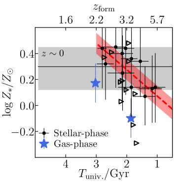
Figure 9.— Observed stellar metallicity as a function of the formation time, or $z_{\rm form}$ (black circles/triangles for those with an upper limit in age estimate). The linear fit with a slope ($0.20\pm 0.08$ dex/Gyr) and standard deviation ($\sigma\sim 0.16$ dex) is shown (red dashed line and shaded region). The local metallicity value of massive galaxies ($\log M_{*}/M_{\odot}\sim 11.5$; Gallazzi et al., 2005) is shown for comparison (gray shaded region). Gas-phase metallicity measurements of massive galaxies ($\log M_{*}/M_{\odot}=11.5$) at similar redshifts (Maiolino et al., 2008) are shown (blue stars), after being calibrated to the local $Z_{*}$ measurement (Section 5.3).

5.3. Redshift Evolution of Stellar-phase Metallicity

While our mass-metallicity relation indicates that galaxies are already enriched to the value at present day (Figure 8), their origin and observed scatter, especially those with small metallicity, is yet to be investigated. We investigate the redshift evolution of total metallicity as a population by considering the formation time ($z_{\rm form}$), which is derived with the mass-weighted age and observed redshift, $T_{\rm form}=T(z_{\rm form})=T(z_{\rm obs})-T_{*}$ (i.e. lookback time to the half-mass time).

In Figure 9, we show the distribution of metallicity as a function of $T_{\rm form}$. A clear correlation between $T_{\rm form}$ and observed metallicity is observed. A linear regression reveals a slope of $\log Z_{*}/dt\sim 0.20\pm{0.08}$ dex/Gyr, with a standard deviation of $\sim 0.15$ dex. Our result shows the metallicity enrichment happening in this class of massive galaxies, whose metallicity already reaches the local value at $z\sim 3$, for the first time.

One may suspect that this is an artifact from the age-metallicity degeneracy. While some galaxies show a weak correlation between the two parameters, the degree of correlation is much smaller than the quoted error bars in Figure 9. Our simulation test also revealed that the total metallicity/age are reproduced reliably enough for the observe trend (see Appendix A).

Interestingly, the linear regression suggests that the metallicity even exceeds the local value of the most massive galaxies in Gallazzi et al. (2005) by $\sim 0.1$ dex. As noted before, our sample galaxies are biased to compact, high density galaxies due to high S/N requirement for the SED fitting. While compact massive galaxies are rare at $z\sim 0$ (Taylor et al., 2010, but see also Poggianti et al. 2013), following events such as minor mergers/second bursts in the following $\sim 10$ Gyr would resolve the tension. We discuss this in the following section.

In Figure 9, we also plot gas-phase metallicity measurements of star forming galaxies in a similar redshift range for comparison. We use the formula derived in Maiolino et al. (2008) at the same mass ($\log M_{*}/M_{\odot}=11.5$). We match the gas-phase metallicity measurement to the stellar metallicity at $z\sim 0$. While comparing absolute values of two different metallicities is extremely challenging due to a number of uncertainties in each measurement (e.g., Sánchez et al., 2017; Bian et al., 2018), the matching process is reasonable for our purpose here, i.e. comparison of relative differences at $z\sim 0$ and $2$.

It is interesting to find an offset of $\sim 0.2$-0.3 dex between those metallicity measurements in our redshift range, that may give us a clue to how massive quenched galaxies enrich metallicity in this redshift. Assuming those star forming galaxies are star forming counterparts of our passive galaxies, the observed gap has to be resolved between half-mass time (i.e. $T_{*}$ ago) and time when they are observed as quenched galaxies.

One possible explanation is the continuation of a low-level star formation activity in a closed box, or “strangulation” (Larson et al., 1980; Peng et al., 2015). Peng et al. (2015) demonstrated in their chemical evolution model that the observed offset in metallicity of local massive star forming and passive galaxies ($\sim 0.1$ dex) can be explained by strangulation. Rapid cessation of star formation by AGN/stellar feedback would instead reproduce a similar metallicity for the two populations. Recent observations in fact revealed low star formation activity (e.g., Gobat et al., 2017; Belli et al., 2017), as well as remaining gas (Gobat et al., 2018, but also Sargent et al. 2015; Bezanson et al. 2019), in massive quiescent galaxies at $z\sim 2$, implying the continuation of star formation after they have formed a large amount of stars, or quenched. In addition, the closed-box enrichment seems to be a good agreement with the observed individual SFHs (Figure 3), independently supporting our speculation here.

However, more detailed chemical modelings would be required to reach a conclusion. For example, the observed gap may also be attributed to the dilution of gas-phase metallicity by infalling pristine gas, while there is no gas infall in quenched galaxies due to virial shock heating (e.g., Birnboim & Dekel, 2003). If this is the case, it is suggested that galaxy quenching may be largely caused by termination of gas infall (e.g., Feldmann & Mayer, 2015), while it is not likely that cutting the gas supply would result in extended SFHs as we observe here. A sophisticated chemical modeling with a panchromatic data set, including gas-mass measurements, would be required for further understanding.

5.4. Following Evolution to $z\sim 0$

We have found that our galaxies are already enriched in metallicity, located on the local mass-metallicity relation. Given the amount of mass and its quiescence, it is within our interests to investigate how these galaxies will evolve to the local population. While there is a large uncertainty to expect their descendant (as described in the Introduction), it is still worth describing their possible paths and mechanisms.

In particular, many members of our sample are compact, high-density galaxies ($\langle r_{\rm eff}\rangle\sim 2$ kpc; possibly due to the selection bias toward high S/Ns). Compact galaxies at these redshifts are often debated in terms of size evolution, where observed size is $\sim 3$–5 times smaller than galaxies at $z\sim 0$ with similar masses (Trujillo et al., 2007; van der Wel et al., 2014; Morishita et al., 2014). While there is still much debate as to whether (all of) these galaxies would follow such a significant size evolution (Nipoti et al., 2012; Newman et al., 2012; Poggianti et al., 2013; Belli et al., 2017), minor merger is a popular mechanism that can efficiently increase their sizes (e.g., Naab et al., 2009; Hopkins et al., 2009; Oser et al., 2010; van Dokkum et al., 2015; Morishita & Ichikawa, 2016).

The scenario appears to consistently work for our result of metallicity, where accretion of low-mass galaxies (which are less-metal-enriched, expected from the mass metallicity relation) would dilute the system’s metallicity to the consistent value. For example, approximately 5 minor mergers, with 1/10 the mass of the host and metallicity inferred from the relation at $z\sim 2$, would lower the host metallicity by $\sim 0.1$ dex, being consistent with the local value. The metallicity gradient observed at $z\sim 0$ (e.g., González Delgado et al., 2014; Martín-Navarro et al., 2018) is independent evidence that such high-$z$ metal-rich galaxies would become cores while the accreted component locates the outer part of local massive galaxies. The integrated metallicity is instead an average value of the whole system; thus, metallicities observed in the local relation should be lower than those observed at higher redshifts.

Infall of metal poor gas associated with minor merging satellites (e.g., Torrey et al., 2012) or direct infall from the cosmic web (Dekel & Birnboim, 2006) would also dilute the system’s total metallicity by inducing the second burst. While it is not clear if the scenario reproduces the observed metallicity gradient at $z\sim 0$, there is a large fraction of early-type galaxies that show an evidence of ongoing star formation at the intermediate redshift (e.g., Treu et al., 2005b; Kaviraj et al., 2011). Spatially resolved studies of such second burst galaxies will shed light on how these different scenarios contribute to the evolutionary path of massive galaxies at high redshift to the local counterpart.

6. Summary

We reconstructed SFHs of 24 massive, passively evolving galaxies at $z\sim 2$. Our new SED modeling with gsf simultaneously fit slitless spectroscopic and photometric data taken from multiple surveys, with no functional assumption for SFHs. Our main findings are as follows.

1. Our massive galaxies have already formed $>50\%$ of their current mass by $\sim 1.5$ Gyr prior to the epoch of observation, with a downsizing trend where more massive galaxies evolve earlier.

2. The SFHs reconstructed by gsf show a more extended feature than what is obtained with a $\tau$-model fitting for most of the sample galaxies, indicating a low-level star formation activity until recently, rather a than abrupt cessation.

3. The stellar-phase metallicities of most of our galaxies are already compatible with local values, indicating a rapid metallicity enrichment being associated with the early stellar-mass formation.

4. By using the reconstructed SFHs and inferred metallicity, we revealed a rapid metallicity enrichment of this class of massive galaxies at a rate of $\sim 0.2$ dex/Gyr in $\log Z_{*}/Z_{\odot}$ from $z\sim 5.5$ to $2.2$.

5. While systematic uncertainties remain, the observed gap between the stellar- and gas-phase metallicities can be explained by continuation of a low-level of star formation in quiescent galaxies and/or dilution of gas-phase metallicity due to the inflow of pristine gas to star forming galaxies. The former scenario is consistent with the finding from individual SFHs.

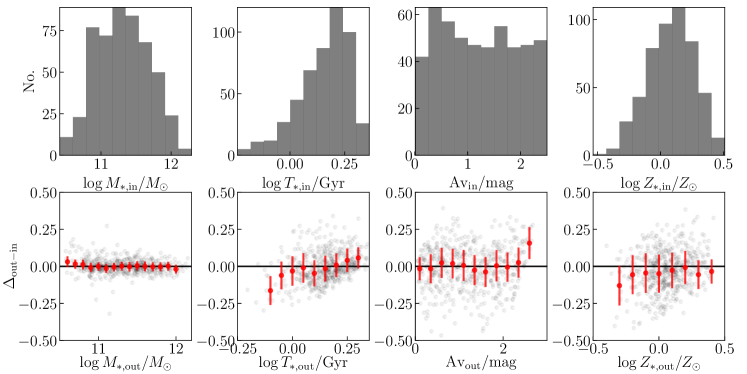
Figure 10.— Top: Parameter distributions of 600 mock galaxies. Noted that age is distributed in a linear scale (peaked at $\sim 1.5$ Gyr), but shown in a log scale here. Bottom: offsets of input and output values ($\Delta_{\rm out-in}$; solid lines represent zero point). Median offsets and 16/84th percentiles range at each output bin are shown (red circles and error bars). Stellar mass, dust attenuation, and mass-weighted metallicity show good agreement for the parameter ranges of our galaxies. While a weak positive correlation is seen in mass-weighted age, the measurement is not biased and scatters are small ($\sigma\sim 0.1$) at the median value of our sample ($\log T_{*}/\,$Gyr$\sim 0.2$).

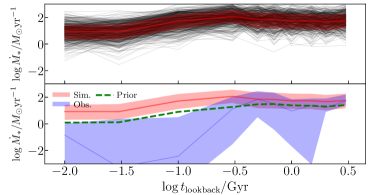
Figure 11.— (Top) Input SFHs (thin lines) used for a simulation in Appendix A, with 16/50/84th percentiles (red hatched region). (Bottom) Median input SFH is compared with the median of observed SFH (blue). Since the simulated SFHs are randomly generated, it does not follow the observed decline at $<0.3$ Gyr. The flat prior used in gsf is shown (dashed line). Its effect should be minimal due to the wide constrain range set in this study ($\pm 3$ dex), as seen in the posterior SFHs deviating from the prior.

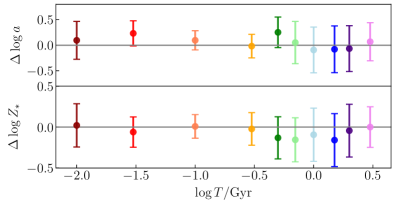
Figure 12.— Mean offsets for amplitude ($\log a_{i,{\rm out}}-\log a_{i,{\rm in}}$; top panels) and metallicity ($\log Z_{i,{\rm out}}-\log Z_{i,{\rm in}}$; bottom panels) with standard deviation at each age pixel from the mock test. The measured standard deviation is added in quadrature to observed uncertainty (i.e. star formation and metallicity histories).

Appendix

Appendix A: Mock Simulation of SED Fitting

We test the fidelity of galaxy SFHs and other parameters with our SED fitting method.

A1: Simulation Setup

To explore parameter spaces we are interested in this study (i.e. quenched galaxies at $z\sim 2$), we set parameters as follows: redshift $z\in[1.6:2.5]$; mass-weighted age $T_{*}/$ Gyr $\in[0.6:2.2]$ peaked at $\sim 1.5$ Gyr; dust attenuation $A_{V}/$mag$\in[0:2.5]$ with a flat distribution; and metallicity $\log Z_{*}/Z_{\odot}\in[-0.5:0.5]$, peaked at $\log Z_{*}/Z_{\odot}=0.15$ dex (top panels of Figure 10). The amplitudes of each template ($a_{i}$; i.e. SFHs) are randomly assigned. The input SFHs are shown in Figure 11.

The mock SEDs are generated via FSPS (Conroy et al., 2009; Conroy & Gunn, 2010) with the assigned parameters. While we provide SFHs at the same time resolution as the fitting templates, this turns out only a small effect, thanks to a sufficient number of age bin (see also Appendix C for the result with higher-resolution SFHs).

Broadband photometry is then extracted by convolving the mock SEDs with filter response curves. For grism spectra, we convolve the mock template with observed line spread function (modeled with a gaussian), which takes into account morphology/instrumental convolution. The error of each spectral element and broadband photometry is randomly assigned based on the observed uncertainty of 24 galaxies in this study ($\sim 5$-20/ pixel at $3700<\lambda_{\rm rest}/{\rm\AA}<4200$; Table Appendix C: Simulation with Realistic SFHs).

No emission lines are added since our focus is the quenched/old galaxy population. In total, 600 mock sets of G102/G141 spectra+broadband photometry are prepared from the template generated with random sets of parameters. We follow the same fitting method as in the main text.

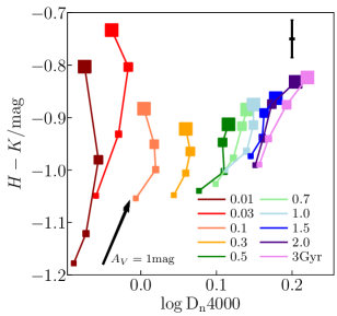
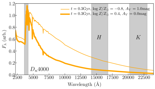
Figure 13.— (Left) Rest-frame NIR color ($H-K$) as a function of ${\rm D_{n}4000}$, for each age (lines with different colors) and metallicity ($\log Z_{*}/Z_{\odot}=-0.8,-0.4,0,0.4$ for small to large symbols). Both parameters are derived from templates that are convolved to a comparable resolution of retrieved grism data ($R\sim 150$), though this is a minimal effect here. Age and metallicity are nearly orthogonal in most of the parameter space, except for the old and solar/supersolar metallicity population at the top right. Typical uncertainties in $H-K$ color and ${\rm D_{n}4000}$ are shown at top right. (Right) example of two spectral templates with similar color and ${\rm D_{n}4000}$ as in the left panel. Despite the similarity, these two templates are distinguishable with photometric data at the optical-to-NIR wavelength range.

A2: Result of Global Parameters

Figure 10 shows the offset of output and input values ($\Delta y=y_{out}-y_{in}$) as a function of output value for major parameters—stellar mass, mass-weighted age, dust attenuation, and metallicity of the mock galaxies. By taking output values (rather than input ones) in $x$-axis, it is possible to infer the false-positive fraction at a given output (i.e. observed) value, and also implement the scatter to observed values for more comprehensive estimate of uncertainty.

We find excellent agreement in stellar mass with scatter of $\sim 0.05$ dex, and moderate agreement in mass-weighted age, dust attenuation, and mass-weighted metallicity with scatters of $\sim 0.11$, $0.14$, and $0.13$ around median values. Median offsets are small for most of parameter ranges. Mass-weighted age shows a negative slope, underestimating for $\sim 0.15$ dex at $\log T\,\hbox to0.0pt{\lower 3.5pt\hbox{$\mathchar 0\relax\sim$}\hss}\raise 1.0pt\hbox{$<$}\,-0.05$. However, most of our sample galaxies dominate higher values, with a median of $\log T_{*}$/ Gyr $\sim 0.2$ (Figure 7), where the bias in parameters is small, and thus we do not correct the offset for our galaxies in the main text.

A3: Result of SFHs

In Figure 12, we summarize offsets of output and input values for amplitude and metallicity at each age pixel to show the fidelity of SFHs and metallicity enrichment histories from all mock galaxies used here. While the offset and scatter may depend on parameter sets with different combinations, this suggests that SFHs can be determined in $\sim 0.5$ dex accuracy.

Metallicity shows a large scatter in reproduced values, with standard deviation of $\sim 0.3$ dex. Given the parameter range assigned for metallicity ($\in[-0.8:0.6]$), we conclude that determination of metallicity at each age pixel is challenging with the current data set. It is noted that this does not mean that reproduced total metallicity has comparable uncertainty, since part of the scatter can be attributed to the age pixel where the total contribution of light is small. Total metallicity, which is light or mass-weighted, should remain less scattered ($\,\hbox to0.0pt{\lower 3.5pt\hbox{$\mathchar 0\relax\sim$}\hss}\raise 1.0pt\hbox{$<$}\,0.2$ dex), as shown in the main text and A2.

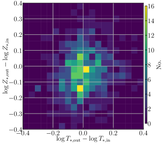
Figure 14.— Distribution of offset of age ($\log T_{*,{\rm out}}-\log T_{*,{\rm in}}$; $x$-axis) and metallicity ($\log Z_{*,{\rm out}}-\log Z_{*,{\rm in}}$; $y$-axis) from our mock test. Color represents the number of galaxies in each grid. The distribution is almost symmetric around the zero point, whereas it would follow a negative slope in case of the age-metallicity degeneracy.

A4: Age-Metallicity Degeneracy

Degeneracy between age and metallicity is notoriously known as one of difficult aspects when modeling accurate SEDs from photometric data (Worthey, 1994). The degeneracy is however resolved once one obtains both information at optical and NIR wavelength range simultaneously (Figure 2; also de Jong, 1996; Smail et al., 2001; Choi et al., 2016).

To see if this is the case for our data set, we first show in the left panel of Figure 13 a rest frame NIR color-${\rm D_{n}4000}$ diagram, both of which are available with our data in this study. Rest frame NIR color ($H-K$) and the strength of 4000 Å (${\rm D_{n}4000}$ Balogh et al., 1999) are calculated with templates used for fitting, which are convolved to a comparable resolution of grism data ($R\sim 150$), including the convolution effect by source morphology. As we see in the figure, age and metallicity are nearly orthogonal in most of the parameter range, meaning the age and metallicity can be well separated from those measurement. The only exception is for old ($\,\hbox to0.0pt{\lower 3.5pt\hbox{$\mathchar 0\relax\sim$}\hss}\raise 1.0pt\hbox{$>$}\,1.5$ Gyr) and solar/super-solar metallicity, where the relation of the two measurements becomes less orthogonal. Due to this, metallicities of our fitting typically have larger uncertainties for old populations.

One may notice that some parameters are not distinguished, especially by the reddening effect by dust (e.g., $t=0.3$ Gyr with $\log Z_{*}/Z_{\odot}=0.4$, $A_{V}=0$ vs. $t=0.3$ Gyr with $\log Z_{*}/Z_{\odot}=-0.8$, $A_{V}=1.0$ mag). However, we stress that to our SED fitting is not relying on any specific colors or indicators, but on all spectrophotometric information over the wide wavelength range. As an example, we show two spectral templates in the right panel of Figure 13, that locate at a similar position in the ${\rm D_{n}4000}$-color space. Despite this, the two templates are clearly distinguishable at rest frame optical to near infrared wavelength range, where sufficient photometric data points are available in this study. Also, photometric error of each flux measurement may affect the SED parameters, but the uncertainty is properly implemented in our fitting framework using MCMC and reflected in the uncertainty range of posterior.

We also investigate the age-metallicity degeneracy with our mock data set. In Figure 14, we show the distribution of offset in total mass-weighted age and metallicity for our mock galaxies. The distribution is symmetric in both axes, whereas the distribution would follow a negative slope if these parameters are degenerated. The distribution is scattered for $\sim 0.2$ dex, which is consistent with those found in A2.

From both tests here, we conclude that the data set used in this study can resolve the age-metallicity degeneracy for our moderately old galaxies ($\,\hbox to0.0pt{\lower 3.5pt\hbox{$\mathchar 0\relax\sim$}\hss}\raise 1.0pt\hbox{$<$}\,2$ Gyr), but star formation and metallicity histories become less certain beyond $T_{\rm lookback}\,\hbox to0.0pt{\lower 3.5pt\hbox{$\mathchar 0\relax\sim$}\hss}\raise 1.0pt\hbox{$>$}\,2$ Gyr.

Appendix B: Comparison of SED Parameters Obtained with Functional SFHs

In Section 4.3, we see that our reconstructed SFHs capture the detail features of individual galaxy SFHs, that are often missed with functional forms. While the deviation is clear in these comparison, it is yet to be investigate how different assumption of SFH results in SED parameters. We here compare the best-fit parameters between two types of SFHs.

In Figure 15, we compare the goodness of fit, $\chi^{2}/\nu$, and major parameters from SED fitting, i.e. stellar mass, light-weighted age and metallicity, and dust attenuation. These values are compared between those reproduced by gsf (main text) and functional ones. Firstly, the goodness of fit is better with gsf for most of our galaxies, which is reasonable given the flexibility of its modeling. We also find that the $\tau$-model ($\propto\exp[-t/\tau]$) is more sensitive to the light from young stellar populations, where the model systematically underestimates system’s ages for $\sim 0.3$ Gyr on average (top panels). The discrepancy propagates to other parameters, where we find over estimated dust attenuation ($\sim 0.3$ mag) and largely underestimated metallicity.

The discrepancy in age and dust becomes slightly smaller when the delayed-$\tau$ model ($\propto t\exp[-t/\tau]$) is used (bottom panels of Figure 15). This is shown in the goodness of fit, where the delayed-$\tau$ model results in smaller values of $\chi^{2}/\,\nu$ (see also Pacifici et al., 2016). This is partly attributed to its rising slope in SFHs, which makes the age slightly older and cancel out discrepancy in other parameters. A large discrepancy in metallicity, however, still remains.

Despite this, it is interesting that the reproduced stellar mass is very consistent with each other, with only $\sim 0.1$ dex scatter in $\log M_{*}$ among our sample. While it is challenging to comprehensively understand this agreement because of a large number of parameters here, this is partly due to the sufficient wavelength coverage to the rest-frame near-IR region, where the light from low-mass stars dominates and less sensitive to other parameters (e.g., Bell et al., 2003). The contribution from other parameters (i.e. age/metallicity/dust) are cancelled out within partial degeneracy at a given form of star formation history. However, this does not necessarily mean that the typical error in stellar mass remains comparably small. As shown in the main text and Appendix A, the stellar mass measurement with gsf accompanies with $\sim 0.2$ dex uncertainty, that is mainly originated from systematics in estimating accurate star formation and metallicity enrichment histories (cf. smaller uncertainties in stellar mass with functional form SFHs estimated here). For this reason, we conclude that stellar mass measurement remains, at least, $\sim 0.15$ dex accuracy for our galaxies, and perhaps for other types of galaxies. The best-fit parameters derived with the two functional SFHs are summarized in Table 2 Summary of physical parameters with different SFHs..

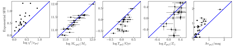
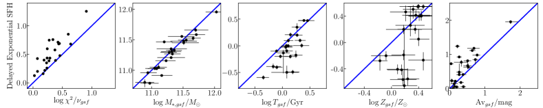
Figure 15.— Comparison of $\chi^{2}/\nu$, and SED parameters for 24 galaxies in this study derived from different SFHs, with gsf ($x$-axis) and with functional forms for SFHs ($y$-axis). The exponential model (top) and delayed (bottom) models are examined. The goodness of fit is better with gsf for most of our sample. While both SFHs reproduce the stellar mass in a good agreement, the functional SFHs overestimate dust attenuation and underestimate age and metallicity. It is noted that age and metallicity of gsf are light-weighted values to match those derived with functional form SFHs, while those in the main text are mass-weighted values.

Appendix C: Simulation with Realistic SFHs

While our test with randomly generated SFHs provides an general idea of the goodness of gsf, there is still concern of how a specific type of SFHs affects output results. In particular, the random SFHs do not fully investigate SFHs of quenched galaxies, i.e. target galaxies of our studies. Upon such a demand, we here repeat a similar fitting analysis as in Appendix A, but with SFHs taken from a cosmological simulation, that gives us an idea how well quenched galaxies are reconstructed within our framework.

In Figure 16, we compare the input and output histories for 10 galaxies. The set of galaxies is selected from the Illustris simulation (Nelson et al., 2015), with a similar mass to our galaxies ($\log M_{*}/M_{\odot}\sim 11$) and quenched at the time of observation (SFR$<1\,M_{\odot}$ / yr at $z\sim 2$). The SFHs, and metallicity enrichment histories, are provided to FSPS, to synthesize SEDs. From the generated SEDs, we extract fluxes corresponding to our grism elements (convolved with morphology of one of our sources) and broadband filters. We then add noise with a conservative value of $\langle{\rm S/N}\rangle=10$ at 4200-5000 Å(and 15 as a supplemental test). We set the observed redshift to $z=2$ and $A_{V}=0.5$ mag uniformly for the sake of simplicity, but this hardly affects the conclusion here.

In general, the posterior captures the feature of SFHs—the peak time of SFR and its length—, and gives fairly good estimates of SED parameters: stellar mass, mass-weight age and metallicity, and dust attenuation (bottom panel of Figure 16). There is a trend that gsf underestimates the star formation in the oldest bin. This leads to underestimation in the mass-weight age for old galaxies with $\log T_{*,\rm input}/{\rm Gyr}>0.2$, but this is only for a small amount ($<0.1$ dex). The offset seen in output metallicity is also small ($\sim 0.1$ dex), and hardly change our conclusion in the main text, as the measurements in the main text quote much larger uncertainties from the analysis in Appendix A.

One caveat is that dust attenuation is overestimated for $\sim 0.2$ mag (and stellar mass is overestimated for $\sim 0.1$ dex accordingly). However, this should be considered as a result of this specific type of SFHs (and SEDs), as we see fairly good reproduction of the parameter for random SFHs in Figure 10. The offset becomes smaller by increasing the input S/N to 15, but is not completely dismissed.

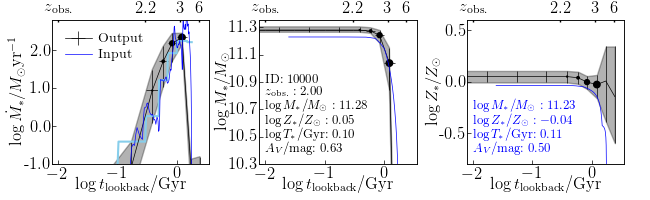
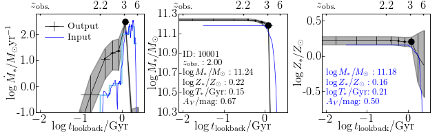
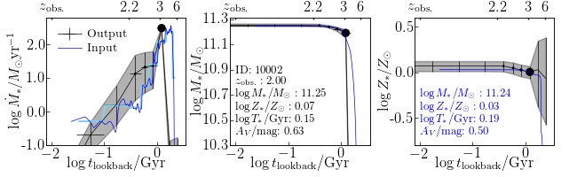
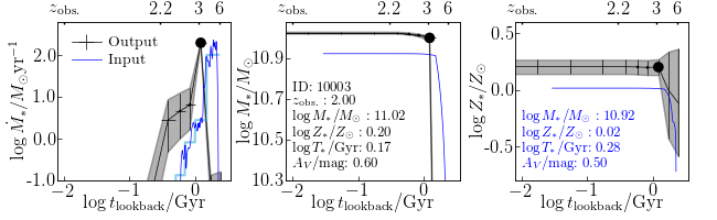
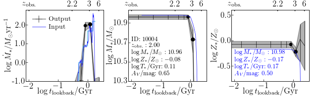
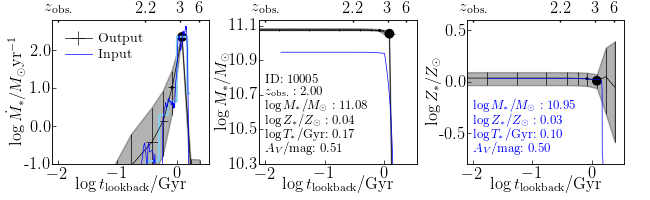
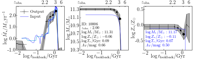
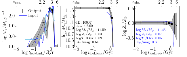
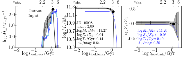
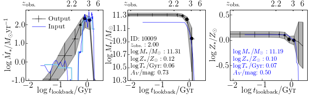
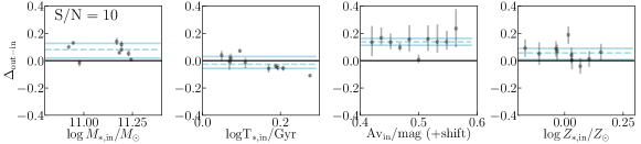
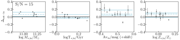
Figure 16.— (Top) Results of the star formation reconstruction with gsf for 10 quenching galaxies. The input star formation and metallicity histories (blue lines) are selected from the Illustris simulation within our observed mass range ($\log M_{*}/M_{\odot}\sim 11$) and quenched (${\rm SFR}<1\,M_{\odot}$/yr) at $z\sim 2$. The SFHs binned to the fitting template resolution are also shown (light blue) for the comparison with output SFHs. The input and output values for each parameters are shown in the inset (blue and black text, respectively). (Bottom) Summary results of output parameters (${\rm\langle S/N\rangle}=10$ and 15). There is a negative trend in mass-weighted age. This is caused by underestimation of star formation in the oldest bin, but the net effect is small ($\Delta T\sim 0.1$ Gyr). The dust attenuation shows an offset ($\Delta\sim 0.2$ mag), but this is rather dependent on a specific type of SFHs (cf. Figure 10).

Table 1Summary of physical parameters.

Obj. ID	R.A.	Decl.	$z_{\rm grism}$	$\log M_{*}$	$\log Z_{*}$	$\log T_{*}$	$A_{V}$	$U-V$	$V-J$	S/N${}^{\rm a}$		${t_{\rm G102}}^{\rm b}$	${t_{\rm G141}}^{\rm b}$
	(deg)	(deg)		($M_{\odot}$)	$(Z_{\odot})^{\rm c}$	(Gyr)	(mag)	(mag)	(mag)	Blue	Red	(s)	(s)
MACS J1149.6$+$2223${}^{\rm d}$
00141	1.77403e$+02$	2.24185e$+01$	$1.96_{-0.01}^{+0.01}$	$11.21_{-0.14}^{+0.13}$	$0.43_{-0.20}^{+0.18}$	$-0.25_{-0.12}^{+0.11}$	$1.72_{-0.15}^{+0.20}$	$1.79_{-0.01}^{+0.01}$	$1.35_{-0.07}^{+0.10}$	4.2	24.5	9529	75987
00227	1.77407e$+02$	2.24162e$+01$	$2.41_{-0.01}^{+0.01}$	$10.94_{-0.13}^{+0.15}$	$-0.28_{-0.17}^{+0.19}$	$0.23_{-0.14}^{+0.14}$	$0.74_{-0.08}^{+0.07}$	$1.20_{-0.01}^{+0.01}$	$0.81_{-0.05}^{+0.00}$	6.8	17.4	19758	80399

GOODS-North    06215 1.89029e$+02$ 6.21726e$+01$ $2.30_{-0.02}^{+0.02}$ $11.55_{-0.13}^{+0.13}$ $0.36_{-0.17}^{+0.18}$ $0.01_{-0.09}^{+0.12}$ $0.65_{-0.09}^{+0.08}$ $1.43_{-0.01}^{+0.01}$ $0.83_{-0.01}^{+0.01}$ 2.8 8.5 5011 6117 07276 1.89306e$+02$ 6.21791e$+01$ $2.50_{-0.01}^{+0.01}$ $11.65_{-0.14}^{+0.13}$ $0.14_{-0.20}^{+0.22}$ $0.20_{-0.10}^{+0.11}$ $0.32_{-0.08}^{+0.08}$ $1.50_{-0.01}^{+0.01}$ $0.77_{-0.01}^{+0.01}$ 6.1 14.1 5011 5011 11470 1.89066e$+02$ 6.21987e$+01$ $1.67_{-0.01}^{+0.01}$ $11.07_{-0.12}^{+0.12}$ $0.33_{-0.17}^{+0.19}$ $0.08_{-0.11}^{+0.09}$ $0.13_{-0.09}^{+0.10}$ $1.17_{-0.01}^{+0.01}$ $0.50_{-0.01}^{+0.01}$ 3.0 20.1 10023 8723 17599 1.89121e$+02$ 6.22289e$+01$ $2.15_{-0.01}^{+0.01}$ $11.16_{-0.15}^{+0.15}$ $0.23_{-0.24}^{+0.25}$ $0.17_{-0.10}^{+0.12}$ $0.41_{-0.10}^{+0.10}$ $1.77_{-0.17}^{+0.12}$ $0.86_{-0.03}^{+0.03}$ 3.5 20.6 33482 39394 17735 1.89061e$+02$ 6.22290e$+01$ $1.84_{-0.01}^{+0.01}$ $11.33_{-0.13}^{+0.13}$ $0.36_{-0.17}^{+0.17}$ $0.14_{-0.16}^{+0.14}$ $0.50_{-0.10}^{+0.11}$ $1.46_{-0.01}^{+0.01}$ $0.83_{-0.00}^{+0.00}$ 3.8 23.5 5011 8123 19341 1.89087e$+02$ 6.22367e$+01$ $1.86_{-0.01}^{+0.01}$ $10.98_{-0.16}^{+0.14}$ $0.02_{-0.26}^{+0.26}$ $0.29_{-0.09}^{+0.12}$ $0.04_{-0.04}^{+0.07}$ $1.19_{-0.01}^{+0.01}$ $0.57_{-0.01}^{+0.01}$ 4.1 31.1 5011 38494 19850 1.89090e$+02$ 6.22392e$+01$ $1.86_{-0.01}^{+0.01}$ $11.06_{-0.16}^{+0.14}$ $0.25_{-0.20}^{+0.23}$ $0.15_{-0.14}^{+0.13}$ $0.53_{-0.15}^{+0.13}$ $1.59_{-0.01}^{+0.01}$ $0.90_{-0.01}^{+0.01}$ 2.1 22.2 5011 38494 22774 1.89128e$+02$ 6.22537e$+01$ $2.01_{-0.01}^{+0.01}$ $11.37_{-0.12}^{+0.12}$ $0.14_{-0.19}^{+0.19}$ $0.16_{-0.10}^{+0.12}$ $0.78_{-0.13}^{+0.10}$ $1.64_{-0.01}^{+0.01}$ $0.97_{-0.01}^{+0.01}$ 2.2 18.4 4811 31476 23006 1.89351e$+02$ 6.22547e$+01$ $2.48_{-0.01}^{+0.01}$ $11.11_{-0.14}^{+0.12}$ $0.11_{-0.20}^{+0.21}$ $0.18_{-0.10}^{+0.11}$ $0.05_{-0.05}^{+0.07}$ $1.27_{-0.01}^{+0.01}$ $0.55_{-0.01}^{+0.01}$ 2.8 8.3 5011 4911 23249 1.89064e$+02$ 6.22560e$+01$ $2.37_{-0.01}^{+0.01}$ $10.89_{-0.14}^{+0.15}$ $0.10_{-0.28}^{+0.25}$ $0.21_{-0.27}^{+0.18}$ $0.34_{-0.22}^{+0.18}$ $1.28_{-0.01}^{+0.01}$ $0.56_{-0.03}^{+0.02}$ 2.9 7.7 5011 15841 24033 1.89115e$+02$ 6.22594e$+01$ $1.67_{-0.01}^{+0.01}$ $11.21_{-0.15}^{+0.14}$ $0.47_{-0.19}^{+0.18}$ $0.19_{-0.10}^{+0.12}$ $0.25_{-0.08}^{+0.09}$ $1.54_{-0.01}^{+0.01}$ $0.87_{-0.00}^{+0.00}$ 3.2 29.2 4811 39494 33780 1.89202e$+02$ 6.23172e$+01$ $1.87_{-0.01}^{+0.01}$ $11.71_{-0.19}^{+0.17}$ $0.48_{-0.20}^{+0.22}$ $0.30_{-0.09}^{+0.08}$ $0.51_{-0.12}^{+0.12}$ $1.92_{-0.01}^{+0.01}$ $1.31_{-0.01}^{+0.01}$ 2.9 14.8 33282 14635    GOODS-South    09704 5.32857e$+01$ -2.78641e$+01$ $1.74_{-0.01}^{+0.01}$ $11.71_{-0.14}^{+0.14}$ $0.40_{-0.18}^{+0.19}$ $0.28_{-0.12}^{+0.12}$ $0.71_{-0.21}^{+0.14}$ $1.69_{-0.02}^{+0.02}$ $1.14_{-0.00}^{+0.00}$ 12.5 17.4 98073 4711 23073 5.31231e$+01$ -2.78034e$+01$ $2.34_{-0.01}^{+0.01}$ $11.32_{-0.18}^{+0.15}$ $0.34_{-0.21}^{+0.22}$ $0.10_{-0.10}^{+0.10}$ $0.15_{-0.09}^{+0.09}$ $1.46_{-0.01}^{+0.01}$ $0.68_{-0.01}^{+0.01}$ 5.4 11.9 0 9423 24569 5.31588e$+01$ -2.77972e$+01$ $1.90_{-0.01}^{+0.01}$ $11.17_{-0.18}^{+0.16}$ $-0.14_{-0.23}^{+0.25}$ $0.35_{-0.09}^{+0.09}$ $0.20_{-0.08}^{+0.07}$ $1.55_{-0.01}^{+0.00}$ $0.77_{-0.01}^{+0.01}$ 1.0 22.6 103246 23358 31397 5.31410e$+01$ -2.77667e$+01$ $1.91_{-0.01}^{+0.01}$ $11.51_{-0.21}^{+0.21}$ $0.45_{-0.25}^{+0.26}$ $0.15_{-0.10}^{+0.08}$ $0.38_{-0.08}^{+0.10}$ $1.66_{-0.00}^{+0.00}$ $0.94_{-0.00}^{+0.00}$ 5.9 32.3 0 21552 39364 5.30628e$+01$ -2.77265e$+01$ $1.61_{-0.01}^{+0.01}$ $11.53_{-0.21}^{+0.23}$ $0.17_{-0.25}^{+0.23}$ $0.44_{-0.18}^{+0.12}$ $0.22_{-0.07}^{+0.08}$ $1.62_{-0.01}^{+0.01}$ $1.09_{-0.00}^{+0.00}$ 8.9 23.6 27270 8923 41021 5.31874e$+01$ -2.77192e$+01$ $2.32_{-0.01}^{+0.01}$ $11.28_{-0.13}^{+0.12}$ $0.08_{-0.17}^{+0.16}$ $0.16_{-0.12}^{+0.10}$ $0.27_{-0.09}^{+0.09}$ $1.23_{-0.01}^{+0.01}$ $0.54_{-0.01}^{+0.01}$ 4.9 15.7 0 4711 41148 5.31279e$+01$ -2.77189e$+01$ $1.76_{-0.01}^{+0.01}$ $11.47_{-0.21}^{+0.20}$ $0.35_{-0.26}^{+0.26}$ $0.39_{-0.10}^{+0.10}$ $0.08_{-0.07}^{+0.07}$ $1.87_{-0.02}^{+0.02}$ $1.18_{-0.01}^{+0.01}$ 3.4 10.6 23058 4611 41520 5.31527e$+01$ -2.77163e$+01$ $1.60_{-0.01}^{+0.01}$ $11.31_{-0.22}^{+0.25}$ $0.20_{-0.27}^{+0.25}$ $0.46_{-0.18}^{+0.13}$ $0.14_{-0.07}^{+0.07}$ $1.81_{-0.01}^{+0.01}$ $1.18_{-0.00}^{+0.00}$ 4.7 10.2 27470 4711 43005 5.31085e$+01$ -2.77101e$+01$ $1.60_{-0.01}^{+0.01}$ $11.32_{-0.22}^{+0.23}$ $0.38_{-0.25}^{+0.29}$ $0.28_{-0.09}^{+0.10}$ $0.39_{-0.08}^{+0.08}$ $1.82_{-0.01}^{+0.00}$ $1.12_{-0.00}^{+0.00}$ 3.9 13.1 23058 9323 43114 5.30624e$+01$ -2.77069e$+01$ $1.90_{-0.01}^{+0.01}$ $12.06_{-0.20}^{+0.19}$ $0.07_{-0.19}^{+0.21}$ $0.37_{-0.10}^{+0.10}$ $0.27_{-0.07}^{+0.07}$ $1.45_{-0.00}^{+0.00}$ $0.81_{-0.00}^{+0.00}$ 25.2 49.4 27270 7720

Note. —

${}^{\rm a}$Average S /Ns of grism spectral element measured at blue ($3400$–$3800$ Å) and red ($4200$–$5000$ Å) wavelength ranges.

${}^{\rm b}$ Total exposure time in G102 and G141 observations.

${}^{\rm c}Z_{\odot}=0.0142$ (Asplund et al., 2009).

${}^{\rm d}$Stellar masses are corrected for magnifications by the foreground cluster.

Table 2Summary of physical parameters with different SFHs.

Note. —

${}^{\rm a}$Stellar mass and dust attenuation for gsf are listed in Table Appendix C: Simulation with Realistic SFHs.

${}^{\rm b}$Light-weighted metallicity and age, to match those derived with functional SFHs.

References

- Abramson et al. (2018) Abramson, L. E., Newman, A. B., Treu, T., et al. 2018, AJ, 156, 29
- Andrews & Martini (2013) Andrews, B. H., & Martini, P. 2013, ApJ, 765, 140
- Asplund et al. (2009) Asplund, M., Grevesse, N., Sauval, A. J., & Scott, P. 2009, ARA&A, 47, 481
- Balogh et al. (1999) Balogh, M. L., Morris, S. L., Yee, H. K. C., Carlberg, R. G., & Ellingson, E. 1999, ApJ, 527, 54
- Bell et al. (2003) Bell, E. F., McIntosh, D. H., Katz, N., & Weinberg, M. D. 2003, ApJS, 149, 289
- Belli et al. (2014) Belli, S., Newman, A. B., & Ellis, R. S. 2014, ApJ, 783, 117
- Belli et al. (2017) —. 2017, ApJ, 834, 18
- Belli et al. (2019) —. 2019, ApJ, 874, 17
- Bertin & Arnouts (1996) Bertin, E., & Arnouts, S. 1996, A&AS, 117, 393
- Bezanson et al. (2019) Bezanson, R., Spilker, J., Williams, C. C., et al. 2019, ApJ, 873, L19
- Bian et al. (2018) Bian, F., Kewley, L. J., & Dopita, M. A. 2018, ApJ, 859, 175
- Birnboim & Dekel (2003) Birnboim, Y., & Dekel, A. 2003, MNRAS, 345, 349
- Boquien et al. (2014) Boquien, M., Buat, V., & Perret, V. 2014, A&A, 571, A72
- Brammer (2018) Brammer, G. 2018, gbrammer/grizli: Preliminary release, doi:10.5281/zenodo.1146905
- Brammer et al. (2016) Brammer, G. B., Marchesini, D., Labbé, I., et al. 2016, ApJS, 226, 6
- Calzetti et al. (2000) Calzetti, D., Armus, L., Bohlin, R. C., et al. 2000, ApJ, 533, 682
- Carnall et al. (2018) Carnall, A. C., Leja, J., Johnson, B. D., et al. 2018, ArXiv e-prints, arXiv:1811.03635
- Chauke et al. (2018) Chauke, P., van der Wel, A., Pacifici, C., et al. 2018, ApJ, 861, 13
- Choi et al. (2014) Choi, J., Conroy, C., Moustakas, J., et al. 2014, ApJ, 792, 95
- Choi et al. (2016) Choi, J., Dotter, A., Conroy, C., et al. 2016, ApJ, 823, 102
- Cid Fernandes (2018) Cid Fernandes, R. 2018, ArXiv e-prints, arXiv:1807.10423
- Cid Fernandes et al. (2005) Cid Fernandes, R., Mateus, A., Sodré, L., Stasińska, G., & Gomes, J. M. 2005, MNRAS, 358, 363
- Cimatti et al. (2004) Cimatti, A., Daddi, E., Renzini, A., et al. 2004, Nature, 430, 184
- Cole et al. (2001) Cole, S., Norberg, P., Baugh, C. M., et al. 2001, MNRAS, 326, 255
- Conroy (2013) Conroy, C. 2013, ARA&A, 51, 393
- Conroy & Gunn (2010) Conroy, C., & Gunn, J. E. 2010, ApJ, 712, 833
- Conroy et al. (2009) Conroy, C., Gunn, J. E., & White, M. 2009, ApJ, 699, 486
- Cowie et al. (1996) Cowie, L. L., Songaila, A., Hu, E. M., & Cohen, J. G. 1996, AJ, 112, 839
- Daddi et al. (2005) Daddi, E., Renzini, A., Pirzkal, N., et al. 2005, ApJ, 626, 680
- de Jong (1996) de Jong, R. S. 1996, A&A, 313, 377
- Dekel & Birnboim (2006) Dekel, A., & Birnboim, Y. 2006, MNRAS, 368, 2
- Diemer et al. (2017) Diemer, B., Sparre, M., Abramson, L. E., & Torrey, P. 2017, ApJ, 839, 26
- Domínguez Sánchez et al. (2016) Domínguez Sánchez, H., Pérez-González, P. G., Esquej, P., et al. 2016, MNRAS, 457, 3743
- Dressler & Gunn (1983) Dressler, A., & Gunn, J. E. 1983, ApJ, 270, 7
- Dressler et al. (2018) Dressler, A., Kelson, D. D., & Abramson, L. E. 2018, ArXiv e-prints, arXiv:1805.04110
- Dressler et al. (2016) Dressler, A., Kelson, D. D., Abramson, L. E., et al. 2016, ApJ, 833, 251
- Erb et al. (2006) Erb, D. K., Shapley, A. E., Pettini, M., et al. 2006, ApJ, 644, 813
- Estrada-Carpenter et al. (2018) Estrada-Carpenter, V., Papovich, C., Momcheva, I., et al. 2018, ArXiv e-prints, arXiv:1810.02824
- Feldmann & Mayer (2015) Feldmann, R., & Mayer, L. 2015, MNRAS, 446, 1939
- Ferreras et al. (2012) Ferreras, I., Pasquali, A., Khochfar, S., et al. 2012, AJ, 144, 47
- Ferreras et al. (2019) Ferreras, I., Pasquali, A., Pirzkal, N., et al. 2019, MNRAS, 486, 1358
- Foreman-Mackey et al. (2013) Foreman-Mackey, D., Hogg, D. W., Lang, D., & Goodman, J. 2013, PASP, 125, 306
- Foreman-Mackey et al. (2014) Foreman-Mackey, D., Sick, J., & Johnson, B. 2014, doi:10.5281/zenodo.12157
- Fukugita et al. (1996) Fukugita, M., Ichikawa, T., Gunn, J. E., et al. 1996, AJ, 111, 1748
- Gallazzi et al. (2014) Gallazzi, A., Bell, E. F., Zibetti, S., Brinchmann, J., & Kelson, D. D. 2014, ApJ, 788, 72
- Gallazzi et al. (2005) Gallazzi, A., Charlot, S., Brinchmann, J., White, S. D. M., & Tremonti, C. A. 2005, MNRAS, 362, 41
- Glazebrook et al. (2017) Glazebrook, K., Schreiber, C., Labbé, I., et al. 2017, Nature, 544, 71
- Gobat et al. (2017) Gobat, R., Daddi, E., Strazzullo, V., et al. 2017, A&A, 599, A95
- Gobat et al. (2018) Gobat, R., Daddi, E., Magdis, G., et al. 2018, Nature Astronomy, 2, 239
- González Delgado et al. (2014) González Delgado, R. M., Cid Fernandes, R., García-Benito, R., et al. 2014, ApJ, 791, L16
- Grogin et al. (2011) Grogin, N. A., Kocevski, D. D., Faber, S. M., et al. 2011, ApJS, 197, 35
- Hamann & Ferland (1999) Hamann, F., & Ferland, G. 1999, ARA&A, 37, 487
- Harikane et al. (2019) Harikane, Y., Ouchi, M., Ono, Y., et al. 2019, arXiv e-prints, arXiv:1902.09555
- Heavens et al. (2004) Heavens, A., Panter, B., Jimenez, R., & Dunlop, J. 2004, Nature, 428, 625
- Hopkins et al. (2009) Hopkins, P. F., Hernquist, L., Cox, T. J., Keres, D., & Wuyts, S. 2009, ApJ, 691, 1424
- Iyer & Gawiser (2017) Iyer, K., & Gawiser, E. 2017, ApJ, 838, 127
- Jimenez et al. (2007) Jimenez, R., Bernardi, M., Haiman, Z., Panter, B., & Heavens, A. F. 2007, ApJ, 669, 947
- Juneau et al. (2014) Juneau, S., Bournaud, F., Charlot, S., et al. 2014, ApJ, 788, 88
- Kauffmann et al. (2003) Kauffmann, G., Heckman, T. M., White, S. D. M., et al. 2003, MNRAS, 341, 33
- Kaviraj et al. (2011) Kaviraj, S., Tan, K.-M., Ellis, R. S., & Silk, J. 2011, MNRAS, 411, 2148
- Kelly et al. (2015) Kelly, P. L., Rodney, S. A., Treu, T., et al. 2015, Science, 347, 1123
- Kelly et al. (2016) Kelly, P. L., Brammer, G., Selsing, J., et al. 2016, ApJ, 831, 205
- Kelson et al. (2014) Kelson, D. D., Williams, R. J., Dressler, A., et al. 2014, ApJ, 783, 110
- Kennicutt (1998) Kennicutt, Jr., R. C. 1998, ARA&A, 36, 189
- Kewley & Ellison (2008) Kewley, L. J., & Ellison, S. L. 2008, ApJ, 681, 1183
- Kirby et al. (2013) Kirby, E. N., Cohen, J. G., Guhathakurta, P., et al. 2013, ApJ, 779, 102
- Koekemoer et al. (2011) Koekemoer, A. M., Faber, S. M., Ferguson, H. C., et al. 2011, ApJS, 197, 36
- Kriek et al. (2009) Kriek, M., van Dokkum, P. G., Labbé, I., et al. 2009, ApJ, 700, 221
- Kriek et al. (2016) Kriek, M., Conroy, C., van Dokkum, P. G., et al. 2016, Nature, 540, 248
- Larson et al. (1980) Larson, R. B., Tinsley, B. M., & Caldwell, C. N. 1980, ApJ, 237, 692
- Leethochawalit et al. (2018) Leethochawalit, N., Kirby, E. N., Moran, S. M., Ellis, R. S., & Treu, T. 2018, ApJ, 856, 15
- Lehner et al. (2016) Lehner, N., O’Meara, J. M., Howk, J. C., Prochaska, J. X., & Fumagalli, M. 2016, ApJ, 833, 283
- Leja et al. (2018) Leja, J., Carnall, A. C., Johnson, B. D., Conroy, C., & Speagle, J. S. 2018, ArXiv e-prints, arXiv:1811.03637
- Lonoce et al. (2015) Lonoce, I., Longhetti, M., Maraston, C., et al. 2015, MNRAS, 454, 3912
- Lotz et al. (2011) Lotz, J. M., Jonsson, P., Cox, T. J., et al. 2011, ApJ, 742, 103
- Lotz et al. (2017) Lotz, J. M., Koekemoer, A., Coe, D., et al. 2017, ApJ, 837, 97
- Maiolino et al. (2008) Maiolino, R., Nagao, T., Grazian, A., et al. 2008, A&A, 488, 463
- Man & Belli (2018) Man, A., & Belli, S. 2018, Nature Astronomy, 2, 695
- Mannucci et al. (2010) Mannucci, F., Cresci, G., Maiolino, R., Marconi, A., & Gnerucci, A. 2010, MNRAS, 408, 2115
- Marsan et al. (2015) Marsan, Z. C., Marchesini, D., Brammer, G. B., et al. 2015, ApJ, 801, 133
- Martín-Navarro et al. (2018) Martín-Navarro, I., Vazdekis, A., Falcón-Barroso, J., et al. 2018, MNRAS, 475, 3700
- McDermid et al. (2015) McDermid, R. M., Alatalo, K., Blitz, L., et al. 2015, MNRAS, 448, 3484
- Momcheva et al. (2016) Momcheva, I. G., Brammer, G. B., van Dokkum, P. G., et al. 2016, ApJS, 225, 27
- Morishita & Ichikawa (2016) Morishita, T., & Ichikawa, T. 2016, ApJ, 816, 87
- Morishita et al. (2014) Morishita, T., Ichikawa, T., & Kajisawa, M. 2014, ApJ, 785, 18
- Morishita et al. (2015) Morishita, T., Ichikawa, T., Noguchi, M., et al. 2015, ApJ, 805, 34
- Morishita et al. (2017) Morishita, T., Abramson, L. E., Treu, T., et al. 2017, ApJ, 835, 254
- Morishita et al. (2018) —. 2018, ApJ, 856, L4
- Muna et al. (2016) Muna, D., Alexander, M., Allen, A., et al. 2016, ArXiv e-prints, arXiv:1610.03159
- Muzzin et al. (2013) Muzzin, A., Marchesini, D., Stefanon, M., et al. 2013, ApJ, 777, 18
- Naab et al. (2009) Naab, T., Johansson, P. H., & Ostriker, J. P. 2009, ApJ, 699, L178
- Nelson et al. (2015) Nelson, D., Pillepich, A., Genel, S., et al. 2015, Astronomy and Computing, 13, 12
- Newman et al. (2012) Newman, A. B., Ellis, R. S., Bundy, K., & Treu, T. 2012, ApJ, 746, 162
- Newville et al. (2017) Newville, M., Nelson, A., Ingargiola, A., et al. 2017, doi:10.5281/zenodo.802298
- Nipoti et al. (2012) Nipoti, C., Treu, T., Leauthaud, A., et al. 2012, MNRAS, 422, 1714
- Oesch et al. (2016) Oesch, P. A., Brammer, G., van Dokkum, P. G., et al. 2016, ApJ, 819, 129
- Oesch et al. (2018) Oesch, P. A., Montes, M., Reddy, N., et al. 2018, ArXiv e-prints, arXiv:1806.01853
- Oke & Gunn (1983) Oke, J. B., & Gunn, J. E. 1983, ApJ, 266, 713
- Onodera et al. (2012) Onodera, M., Renzini, A., Carollo, M., et al. 2012, ApJ, 755, 26
- Onodera et al. (2015) Onodera, M., Carollo, C. M., Renzini, A., et al. 2015, The Astrophysical Journal, 808, 161
- Onodera et al. (2016) Onodera, M., Carollo, C. M., Lilly, S., et al. 2016, ApJ, 822, 42
- Oser et al. (2010) Oser, L., Ostriker, J. P., Naab, T., Johansson, P. H., & Burkert, A. 2010, ApJ, 725, 2312
- Osterbrock (1989) Osterbrock, D. E. 1989, Astrophysics of gaseous nebulae and active galactic nuclei
- Pacifici et al. (2016) Pacifici, C., Kassin, S. A., Weiner, B. J., et al. 2016, ApJ, 832, 79
- Panter et al. (2007) Panter, B., Jimenez, R., Heavens, A. F., & Charlot, S. 2007, MNRAS, 378, 1550
- Panter et al. (2008) —. 2008, MNRAS, 391, 1117
- Peng et al. (2015) Peng, Y., Maiolino, R., & Cochrane, R. 2015, Nature, 521, 192
- Pirzkal et al. (2017) Pirzkal, N., Malhotra, S., Ryan, R. E., et al. 2017, ApJ, 846, 84
- Poggianti et al. (2013) Poggianti, B. M., Calvi, R., Bindoni, D., et al. 2013, ApJ, 762, 77
- Postman et al. (2012) Postman, M., Coe, D., Benítez, N., et al. 2012, ApJS, 199, 25
- Riechers et al. (2013) Riechers, D. A., Bradford, C. M., Clements, D. L., et al. 2013, Nature, 496, 329
- Salpeter (1955) Salpeter, E. E. 1955, ApJ, 121, 161
- Sánchez et al. (2017) Sánchez, S. F., Barrera-Ballesteros, J. K., Sánchez-Menguiano, L., et al. 2017, MNRAS, 469, 2121
- Sargent et al. (2015) Sargent, M. T., Daddi, E., Bournaud, F., et al. 2015, ApJ, 806, L20
- Schawinski et al. (2014) Schawinski, K., Urry, C. M., Simmons, B. D., et al. 2014, MNRAS, 440, 889
- Schmidt et al. (2014) Schmidt, K. B., Treu, T., Brammer, G. B., et al. 2014, ApJ, 782, L36
- Schreiber et al. (2018) Schreiber, C., Glazebrook, K., Nanayakkara, T., et al. 2018, ArXiv e-prints, arXiv:1807.02523
- Skelton et al. (2014) Skelton, R. E., Whitaker, K. E., Momcheva, I. G., et al. 2014, ApJS, 214, 24
- Smail et al. (2001) Smail, I., Kuntschner, H., Kodama, T., et al. 2001, MNRAS, 323, 839
- Snyder et al. (2017) Snyder, G. F., Lotz, J. M., Rodriguez-Gomez, V., et al. 2017, MNRAS, 468, 207
- Straatman et al. (2014) Straatman, C. M. S., Labbé, I., Spitler, L. R., et al. 2014, ApJ, 783, L14
- Tacconi et al. (2008) Tacconi, L. J., Genzel, R., Smail, I., et al. 2008, ApJ, 680, 246
- Taylor et al. (2010) Taylor, E. N., Franx, M., Glazebrook, K., et al. 2010, ApJ, 720, 723
- Teplitz et al. (2013) Teplitz, H. I., Rafelski, M., Kurczynski, P., et al. 2013, AJ, 146, 159
- Thomas et al. (2003) Thomas, D., Maraston, C., & Bender, R. 2003, MNRAS, 339, 897
- Thomas et al. (2005) Thomas, D., Maraston, C., Bender, R., & Mendes de Oliveira, C. 2005, ApJ, 621, 673
- Thomas et al. (2010) Thomas, D., Maraston, C., Schawinski, K., Sarzi, M., & Silk, J. 2010, MNRAS, 404, 1775
- Toft et al. (2014) Toft, S., Smolčić, V., Magnelli, B., et al. 2014, ApJ, 782, 68
- Tojeiro et al. (2007) Tojeiro, R., Heavens, A. F., Jimenez, R., & Panter, B. 2007, MNRAS, 381, 1252
- Tomczak et al. (2014) Tomczak, A. R., Quadri, R. F., Tran, K.-V. H., et al. 2014, ApJ, 783, 85
- Torrey et al. (2012) Torrey, P., Cox, T. J., Kewley, L., & Hernquist, L. 2012, ApJ, 746, 108
- Torrey et al. (2017) Torrey, P., Wellons, S., Ma, C.-P., Hopkins, P. F., & Vogelsberger, M. 2017, MNRAS, 467, 4872
- Trager et al. (2000) Trager, S. C., Faber, S. M., Worthey, G., & González, J. J. 2000, AJ, 119, 1645
- Tremonti et al. (2004) Tremonti, C. A., Heckman, T. M., Kauffmann, G., et al. 2004, ApJ, 613, 898
- Treu et al. (2005a) Treu, T., Ellis, R. S., Liao, T. X., & van Dokkum, P. G. 2005a, ApJ, 622, L5
- Treu et al. (2005b) Treu, T., Ellis, R. S., Liao, T. X., et al. 2005b, ApJ, 633, 174
- Treu et al. (2015) Treu, T., Schmidt, K. B., Brammer, G. B., et al. 2015, ApJ, 812, 114
- Troncoso et al. (2014) Troncoso, P., Maiolino, R., Sommariva, V., et al. 2014, A&A, 563, A58
- Trujillo et al. (2007) Trujillo, I., Conselice, C. J., Bundy, K., et al. 2007, MNRAS, 382, 109
- van der Wel et al. (2014) van der Wel, A., Franx, M., van Dokkum, P. G., et al. 2014, ApJ, 788, 28
- van Dokkum et al. (2013a) van Dokkum, P., Brammer, G., Momcheva, I., et al. 2013a, ArXiv e-prints, arXiv:1305.2140
- van Dokkum et al. (2008) van Dokkum, P. G., Franx, M., Kriek, M., et al. 2008, ApJ, 677, L5
- van Dokkum et al. (2010) van Dokkum, P. G., Whitaker, K. E., Brammer, G., et al. 2010, ApJ, 709, 1018
- van Dokkum et al. (2013b) van Dokkum, P. G., Leja, J., Nelson, E. J., et al. 2013b, ApJ, 771, L35
- van Dokkum et al. (2015) van Dokkum, P. G., Nelson, E. J., Franx, M., et al. 2015, ApJ, 813, 23
- Vazdekis et al. (2015) Vazdekis, A., Coelho, P., Cassisi, S., et al. 2015, MNRAS, 449, 1177
- Walcher et al. (2009) Walcher, C. J., Coelho, P., Gallazzi, A., & Charlot, S. 2009, MNRAS, 398, L44
- Walcher et al. (2015) Walcher, C. J., Coelho, P. R. T., Gallazzi, A., et al. 2015, A&A, 582, A46
- Wang et al. (2017) Wang, X., Jones, T. A., Treu, T., et al. 2017, ApJ, 837, 89
- Wang et al. (2018) —. 2018, ArXiv e-prints, arXiv:1808.08800
- Wellons et al. (2015) Wellons, S., Torrey, P., Ma, C.-P., et al. 2015, MNRAS, 449, 361
- Williams et al. (2009) Williams, R. J., Quadri, R. F., Franx, M., van Dokkum, P., & Labbé, I. 2009, ApJ, 691, 1879
- Worthey (1994) Worthey, G. 1994, ApJS, 95, 107
- Wuyts et al. (2012) Wuyts, S., Förster Schreiber, N. M., Genzel, R., et al. 2012, ApJ, 753, 114
- Yabe et al. (2014) Yabe, K., Ohta, K., Iwamuro, F., et al. 2014, MNRAS, 437, 3647
- Yi et al. (1997) Yi, S., Demarque, P., & Oemler, Jr., A. 1997, ApJ, 486, 201
- Younger et al. (2007) Younger, J. D., Fazio, G. G., Huang, J.-S., et al. 2007, ApJ, 671, 1531
- Zahid et al. (2014) Zahid, H. J., Kashino, D., Silverman, J. D., et al. 2014, ApJ, 792, 75
- Zitrin et al. (2015) Zitrin, A., Labbé, I., Belli, S., et al. 2015, ApJ, 810, L12