Stellar ages, masses, and radii from asteroseismic modeling are robust to systematic errors in spectroscopy

Abstract

Context. The search for twins of the Sun and Earth relies on accurate characterization of stellar and the exoplanetary parameters age, mass, and radius. In the modern era of asteroseismology, parameters of solar-like stars are derived by fitting theoretical models to observational data, which include measurements of their oscillation frequencies, metallicity [Fe/H], and effective temperature $T_{\text{eff}}$. Furthermore, combining this information with transit data yields the corresponding parameters for their associated exoplanets.

Aims. While values of [Fe/H] and $T_{\text{eff}}$ are commonly stated to a precision of $\sim$ 0.1 dex and $\sim$ 100 K, the impact of systematic errors in their measurement has not been studied in practice within the context of the parameters derived from them. Here we seek to quantify this.

Methods. We used the Stellar Parameters in an Instant (SPI) pipeline to estimate the parameters of nearly 100 stars observed by Kepler and Gaia, many of which are confirmed planet hosts. We adjusted the reported spectroscopic measurements of these stars by introducing faux systematic errors and, separately, artificially increasing the reported uncertainties of the measurements, and quantified the differences in the resulting parameters.

Results. We find that a systematic error of 0.1 dex in [Fe/H] translates to differences of only 4%, 2%, and 1% on average in the resulting stellar ages, masses, and radii, which are well within their uncertainties ($\sim$ 11%, 3.5%, 1.4%) as derived by SPI. We also find that increasing the uncertainty of [Fe/H] measurements by 0.1 dex increases the uncertainties of the ages, masses, and radii by only 0.01 Gyr, 0.02 $\text{M}_{\odot}$, and 0.01 $\text{R}_{\odot}$, which are again well below their reported uncertainties ($\sim$ 0.5 Gyr, 0.04 $\text{M}_{\odot}$, 0.02 $\text{R}_{\odot}$). The results for $T_{\text{eff}}$ at 100 K are similar.

Conclusions. Stellar parameters from SPI are unchanged within uncertainties by errors of up to 0.14 dex or 175 K. They are even more robust to errors in $T_{\text{eff}}$ than the seismic scaling relations. Consequently, the parameters for their exoplanets are also robust.

1 Introduction

The modern study of cool dwarf stars has been revolutionized in recent years by ultraprecise measurements of low-amplitude global stellar pulsations (for a summary of early results, see Chaplin & Miglio 2013). Traveling through the star before emerging near the surface, pulsations bring information to light about the otherwise opaque conditions of the stellar interior, and thereby provide numerous constraints to the internal structure and composition of stars. Indeed, connecting theoretical stellar models to measurements of pulsation frequencies—as well as other measurements, such as those derived from spectroscopy—yields precise determinations of stellar parameters such as age, mass, and radius (for an overview, see Basu & Chaplin, 2017).

Precisely constrained stellar parameters are broadly useful for a variety of endeavours, such as testing theories of stellar and galactic evolution (e.g., Deheuvels et al., 2016; Hjørringgaard et al., 2017; Nissen et al., 2017; Bellinger et al., 2017) and mapping out history and dynamics of the Galaxy (e.g., Chiappini et al., 2015; Anders et al., 2017; Silva Aguirre et al., 2018; Feuillet et al., 2018). Combining stellar parameters with transit measurements furthermore yields properties of the exoplanets that they harbor, such as their masses, radii, obliquities, eccentricities, and semi-major axes (e.g., Seager & Mallén-Ornelas, 2003; Huber et al., 2013; Van Eylen et al., 2014; Huber, 2016, 2018; Campante et al., 2016; Kamiaka et al., 2018; Adibekyan et al., 2018). This then permits tests to theories of planet formation (e.g., Lin et al., 1996; Watson et al., 2011; Morton & Johnson, 2011; Lai et al., 2011; Guillochon et al., 2011; Thies et al., 2011; Teyssandier et al., 2013; Plavchan & Bilinski, 2013; Matsakos & Königl, 2015, 2017; Li & Winn, 2016; Königl et al., 2017; Gratia & Fabrycky, 2017) and facilitates the search for habitable exoplanets.

From first principles, one may obtain approximate relations to deduce stellar radii ($R$), mean densities ($\rho$), and masses ($M$) from asteroseismic data by scaling the values of the Sun to the observed properties of other stars (“scaling relations,” Ulrich, 1986; Brown et al., 1991; Kjeldsen & Bedding, 1995):

$$\frac{R}{\text{R}_{\odot}} \simeq\left(\frac{\nu_{\max}}{\nu_{\max,\odot}}\right)\left(\frac{\Delta\nu}{\Delta\nu_{\odot}}\right)^{-2}\left(\frac{T_{\text{eff}}}{T_{\text{eff},\odot}}\right)^{\frac{1}{2}}$$ (1)

$$\frac{\rho}{\rho_{\odot}} \simeq\left(\frac{\Delta\nu}{\Delta\nu_{\odot}}\right)^{2}$$ (2)

$$\frac{M}{\text{M}_{\odot}} \simeq\left(\frac{\nu_{\max}}{\nu_{\max,\odot}}\right)^{3}\left(\frac{\Delta\nu}{\Delta\nu_{\odot}}\right)^{-4}\left(\frac{T_{\text{eff}}}{T_{\text{eff},\odot}}\right)^{\frac{3}{2}}.$$ (3)

Here $T_{\text{eff}}$ is the effective temperature of the star, $\nu_{\max}$ is the frequency of maximum oscillation power, and $\Delta\nu$ is the large frequency separation (for detailed definitions, see, e.g., Basu & Chaplin, 2017). The quantities subscripted with the solar symbol ($\odot$) correspond to the solar values: ${\nu_{\max,\odot}=3090\pm 30\leavevmode\nobreak\ \mu\text{Hz}}$, ${\Delta\nu_{\odot}=135.1\pm 0.1\leavevmode\nobreak\ \mu\text{Hz}}$, and ${T_{\text{eff},\odot}=5772.0\pm 0.8\leavevmode\nobreak\ \text{K}}$ (Huber et al., 2011; Prša et al., 2016). This way of estimating stellar parameters is often referred to as the “direct method” (e.g., Lundkvist et al., 2018) because it is independent of stellar models and relies only on physical arguments. We note that there are no such scaling relations for the stellar age.

The mass and radius seismic scaling relations are functions of the stellar effective temperature, which, along with metallicity, can be derived from spectroscopic observations of a star. A variety of factors contribute to the determination of these spectroscopic parameters, such as spectra normalization, corrections for pixel-to-pixel variations, the placement of the continuum, and so on (e.g., Massey & Hanson, 2013; Škoda, 2017). The analysis can be complicated by effects such as line blending and broadening. Uncertainties in atmospheric models and the techniques for obtaining atmospheric parameters such as the measurement of equivalent widths, fitting on synthetic spectra, and degeneracies between spectroscopic parameters can also cause difficulties. Often, parameters for targets in large spectroscopic surveys are extracted automatically without visual inspection, which can lead to poor fits that sometimes go unnoticed. Conversely, analysis based on visual inspection sometimes leads to different practitioners coming to different conclusions about the same star. Thus there are opportunities for systematic errors to be introduced into the determined effective temperatures and metallicities (e.g., Creevey et al., 2013). However, to date, no study has systematically tested in practice the impact of systematic errors in spectroscopic parameters on the determination of stellar parameters for a large sample of stars.

Unlike the effective temperature, the classical scaling relations presented above are not functions of metallicity, and so one would expect metallicity to have little importance in the determination of stellar masses and radii. However, these relations are approximations, and are not perfectly accurate. Several studies (e.g., White et al., 2011; Belkacem et al., 2011; Mathur et al., 2012; Hekker et al., 2013; Mosser et al., 2013; Huber et al., 2014; Guggenberger et al., 2016; Sharma et al., 2016; Gaulme et al., 2016; Huber et al., 2017; Guggenberger et al., 2017; Viani et al., 2017; Themeßl et al., 2018) have sought to quantify the validity of the seismic scaling relations—especially as a function of stellar evolution, when the assumption of solar homology breaks down—for example by comparison with stellar models, or via orbital analyses of binary stars. Viani et al. (2017) have also recently shown theoretically that these relations neglect a term for the mean molecular weight, which implies a previously unaccounted for dependence on metallicity.

To obtain more accurate mass and radius estimates—and stellar ages—one can fit theoretical models to the observations of a star (e.g., Brown et al., 1994; Gai et al., 2011; Metcalfe et al., 2014; Lebreton & Goupil, 2014; Silva Aguirre et al., 2015, 2017; Bellinger et al., 2016). The connection between observations and stellar parameters then becomes much more complex, relying on the details of not only the coupled differential equations governing the structure and evolution of stars, but also the choices and implementations regarding the microphysics of the star, such as the opacities and equation of state of stellar plasma. This motivates the need for numerical studies to determine the relationships between the observations of a star and the resulting fundamental parameters (e.g., Brown et al., 1994; Angelou et al., 2017; Valle et al., 2018). Here we examine one important aspect of these relations: namely, the impact of systematic errors and underestimated uncertainties in spectroscopic parameters on the determination of stellar parameters via asteroseismic modeling.

In order to perform this study, we used the Stellar Parameters in an Instant pipeline (SPI, Bellinger et al., 2016), which uses machine learning to rapidly connect observations of stars to theoretical models. The SPI method involves training an ensemble or “forest” of decision tree regressors (Breiman, 2001; Geurts et al., 2006; Friedman et al., 2001) to learn the relationships between the observable aspects of stars (such as their oscillations) and the unobserved or unobservable aspects (such as their age). We then fed the observations of a particular star into the learned forest, which outputs the desired predicted quantities. In order to propagate the uncertainties of the observations into each of the predicted quantities, we generated random realizations of noise according to the uncertainties of the observations (including their correlations), and ran these random realizations also through the forest. This yields the posterior distribution for each predicted quantity, from which we may obtain, for example, the mean value and its corresponding uncertainty for quantities such as the stellar age, mass, radius, mean density, and luminosity.

Using this approach, one can simultaneously and independently vary multiple free parameters corresponding to uncertain aspects of stellar models, such as the efficiency of convection and the strength of gravitational settling; and therefore propagate many of the uncertainties of the theoretical models into the resulting stellar parameters. To this end, we generated a large grid of stellar models that have been varied in age as well as seven other parameters controlling the physics of the evolution, which is described in more detail in the next section. Since obtaining the parameters of a star with SPI takes less than a minute (rather than hours or days, as is typical with some other methods) we were then able to test the robustness of the final stellar parameters against injections of various amounts of systematic errors.

The question of how systematic errors in spectroscopy impact stellar parameter determinations has direct bearing on exoplanet research. This is due to the fact that the determination of exoplanetary parameters generally depends very strongly on the ability to constrain the parameters of the host star (see Figure 1).

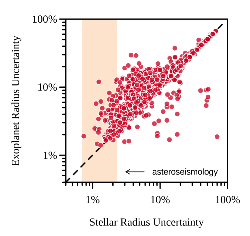
Figure 1: Relative uncertainties of the radii of transiting exoplanets as a function of the relative uncertainty in the radius of their host star. The dashed line shows a one-to-one agreement. The shaded region shows the full range of stellar radii uncertainties determined for the 97 stars examined in this paper. Exoplanet data are taken from the collection by Han et al. (2014).

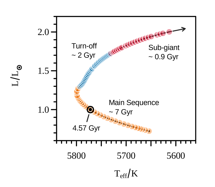
Figure 2: Theoretical evolution of the Sun in the HR diagram. The position of the present-age Sun is given with the solar symbol ($\odot$). The points indicate models that have been selected from the track. They are colored according to their assigned phase of evolution, and the approximate duration of each phase is indicated.

Given the radius of the host star from asteroseismology (e.g., using Equation 1; or using more sophisticated methods, such as SPI), and assuming a uniformly bright stellar disk, the radius of a transiting exoplanet can be found by measuring the transit depth (e.g., Seager & Mallén-Ornelas, 2003). Given the stellar radius and mean density (e.g., Equation 2), and assuming a circular orbit, one can compute the semi-major axis of an exoplanet from its orbital period. Combining that information with the stellar mass (e.g., Equation 3), one can find the mass of an exoplanet using Kepler’s third law. As prevailing theories give that planets form roughly around the same time as the host star, the stellar age that is found is generally then attributed to its companions as well (e.g., Jenkins et al., 2015; Campante et al., 2015; Safonova et al., 2016; Christensen-Dalsgaard & Silva Aguirre, 2018). From this information, the composition of an exoplanet can be determined by connecting these properties to theoretical models of planet structure and formation (e.g., Seager et al., 2007; Weiss & Marcy, 2014; Rogers, 2015; Huber, 2018).

Thus, if the parameters derived for the host star are biased, then so too will be the parameters for its exoplanets. A differential bias—e.g., a bias that affects mass more than radius—would furthermore impact strongly on matters such as empirical mass–radius relations (e.g., Seager et al., 2007; Torres et al., 2010).

2 Methods

We used Modules for Experiments in Stellar Astrophysics (MESA r10108, Paxton et al., 2011, 2013, 2015, 2018) to construct a grid of stellar models following the procedure given by Bellinger et al. (2016). The initial parameters were varied quasi-randomly in the ranges given in Table 1. We introduced an additional free parameter, $\alpha_{uv}$, which controls the efficiency of convective envelope undershooting. As convection is modeled in MESA as a time-dependent diffusive process, under- and over-shooting are achieved by applying convective velocities to zones within a distance of ${\alpha H_{p}}$ beyond the convective boundary, where $\alpha$ is the under- or over-shooting parameter, and $H_{p}$ is the local pressure scale height. The convective velocities that are used are taken from a distance $f_{0}$ before the boundary; here we used ${f_{0}=0.01\leavevmode\nobreak\ H_{p}}$. The remaining aspects of the models are the same as in Bellinger et al. 2016.

Table 1: Parameter ranges for the grid of stellar models. For reference, values corresponding to a solar-calibrated model and also the derived initial spectroscopic parameter ranges are listed as well.

Parameter	Symbol	Range	Solar value
Mass	$M$/M⊙	$(0.7,1.8)$	1
Mixing length	$\alpha_{\text{MLT}}$	$(1,3)$	1.85
Initial helium	$Y_{0}$	$(0.22,0.34)$	0.273
Initial metallicity	$Z_{0}$	$(0.0001,0.04)^{a}$	0.019
Overshoot	$\alpha_{\text{ov}}$	$(0.0001,1)^{a}$	-
Undershoot	$\alpha_{\text{us}}$	$(0.0001,1)^{a}$	$\leq 0.05^{b}$
Diffusion factor	$D$	$(0.0001,3)^{a}$	1
Eff. temperature	$T_{\text{eff}}$	$(4000,14000)$	5772
Metallicity	[Fe/H]	$(-2.2,0.44)$	0

^avaried logarithmically, ^bBasu 1997

We calculated ${N=8\,170}$ evolutionary tracks which we simulated from the zero-age main sequence until either an age of $20\leavevmode\nobreak\ \text{Gyr}$ or an asymptotic period spacing of $150\leavevmode\nobreak\ \text{s}$, which is generally around the base of the red giant branch. Since the initial conditions of the grid are varied quasi-randomly, the resolution in each parameter $x$ is given by ${(x_{\max}-x_{\min})/N}$; e.g., the typical resolution in mass is approximately $0.0001\leavevmode\nobreak\ {\text{M}}_{\odot}$. From each track we obtained 32 models with core hydrogen abundance $X_{c}>0.1$ nearly evenly spaced in age (i.e., main-sequence models), 32 models with $0.1\leq X_{c}\leq 10^{-6}$ nearly evenly spaced in $\log X_{c}$ (turn-off models), and 32 models beyond $X_{c}<10^{-6}$ again nearly evenly spaced in age (sub-giant models). These phases are visualized in Figure 2.

We calculated $p$-mode frequencies for these models using the GYRE oscillation code (Townsend & Teitler, 2013). We obtained frequency separations and ratios (Roxburgh & Vorontsov, 2003) for these models following the procedures given in Bellinger et al. 2016. We removed models where the presence of mixed modes made it impossible to calculate these quantities.

3 Data

We obtained oscillation mode frequencies, $\nu_{\max}$ values, effective temperatures, and metallicities for 97 stars observed by the Kepler spacecraft (Borucki et al., 2010a) from previous studies. Data for 31 of the stars came from the Kepler Ages project (Silva Aguirre et al., 2015; Davies et al., 2016), and 66 were from the Kepler LEGACY project (Lund et al., 2017; Silva Aguirre et al., 2017). The spectroscopic parameters of these stars are visualized in Figure 3. We processed the mode frequencies to obtain asteroseismic frequency separations and ratios in the same way that we processed the theoretical model frequencies in the previous section. These stars are visualized in the so-called CD diagram (Christensen-Dalsgaard, 1984) in Figure 4. The relative uncertainties on the observational constraints for these stars are visualized in Figure 6. This figure furthermore illustrates the observational data we input to SPI.

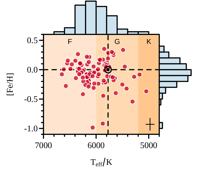
Figure 3: Spectroscopic measurements of 97 solar-like oscillating stars observed by Kepler. Typical uncertainties (0.1 dex, 100 K) are indicated with the cross in the bottom right corner. Histograms are affixed to the top and right side of the figure showing the metallicity and effective temperature distributions for the sample. The values for the Sun are given with the solar symbol ($\odot$). The background colors indicate the spectral type (F, G, K).

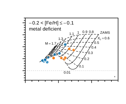
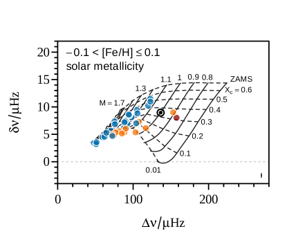
Figure 4: CD diagram showing asteroseismic measurements—the small frequency separation $\delta\nu$ and the the large frequency separation $\Delta\nu$—for the sample of 97 solar-like stars studied here. The panels are arranged by metallicity. The points are colored by spectral type: F (blue, ${T_{\text{eff}}>6000\leavevmode\nobreak\ \text{K}}$), G (orange, ${6000\geq T_{\text{eff}}>5200\leavevmode\nobreak\ \text{K}}$), K (red, ${T_{\text{eff}}\leq 5200\leavevmode\nobreak\ \text{K}}$). The cross in the bottom right corner of each panel shows typical uncertainties (see also Figure 6). The dotted light gray line indicates where ${\delta\nu=0}$. The solid lines trace theoretical tracks of stellar evolution, with each track labeled along the top by its mass (in solar units) and connected by the dashed lines that are spaced in core-hydrogen abundance ($X_{c}$).

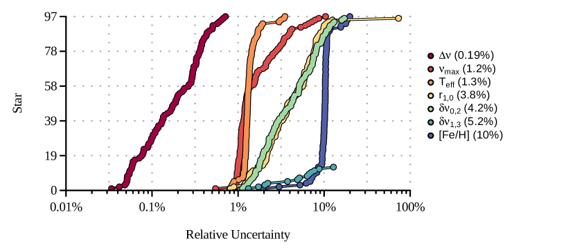
Figure 5: Relative uncertainty of each measurement for each of the 97 stars analyzed here. The uncertainties are given in the sense of $\sigma/\mu$ where $\mu$ is the mean of the estimate and $\sigma$ is the standard deviation—except in the case of [Fe/H], where these quantities are instead given for $\exp($[Fe/H]$)$. For each type of measurement, the order of the stars is given in order of increasing relative uncertainty, so for example Star 1 is not necessarily the same star in all the different types of measurements. We note that $\delta\nu_{1,3}$ measurements are only available for 13 of the stars.

Figure 6: Cumulative distributions showing the relative uncertainty of each estimated stellar parameter for each of the 97 stars, obtained by running the data in Figure 6 through SPI.

For comparison purposes, we additionally obtained luminosity and radius measurements for these stars from the recent Gaia Data Release 2 (DR2, Gaia Collaboration et al., 2018; Andrae et al., 2018). We identified these stars using the 2MASS cross-matched catalog (Marrese et al., 2018) for all except KIC 10514430 and KIC 8379927, which we located using a cone search. We note that these measurements have not been corrected for extinction.

4 Results

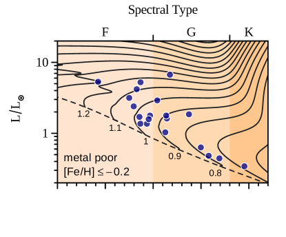
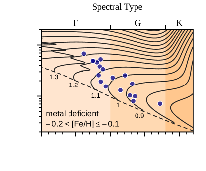
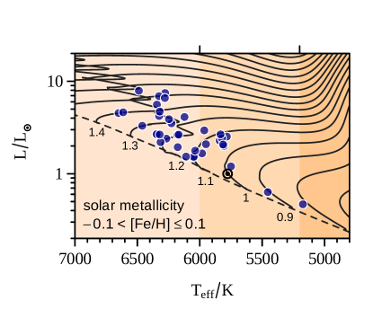
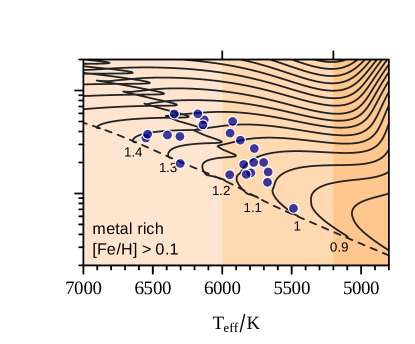
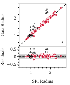
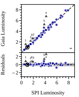
Figure 7: Hertzsprung–Russell diagrams of solar-like stars with temperatures from spectroscopy and predicted luminosities from asteroseismic modeling. The panels are arranged by metallicity, with the lines showing theoretical evolutionary sequences for stars of the corresponding metallicities having the indicated masses (expressed in solar units). The dashed line traces the zero-age main sequence. The background colors indicate the spectral types of the stars (F, G, K). Typical uncertainties are 0.15 $\text{L}_{\odot}$ and 100 K.

Figure 8: Comparison of stellar radii (left) and luminosities (right) in solar units from Gaia observations against those from stellar modeling using the SPI pipeline. Typical uncertainties are shown as error bars in the lower right corners. Each shade of gray in the residual plots represents an average $1\sigma$, ranging from one to three. Stars with estimates significantly different at the ${\sigma>3}$ level are shown as gray triangles. Stars which are outliers in more than one panel are labeled. We note the differences in scale between the left and right panels. The biases in the residuals are consistent with zero ($-0.056\pm 0.091$ $\text{R}_{\odot}$ and $-0.14\pm 0.36$ $\text{L}_{\odot}$)

We applied SPI to the sample of 97 stars using the grid of theoretical models that we generated and the observational constraints shown in Figure 6. Random realizations of the observations that fell outside of the range of the grid of models were dropped. Figure 6 shows the relative uncertainties in the estimated stellar parameters for this sample. The stellar parameters themselves can be found in Table LABEL:tab:parameters in the Appendix. Figure 8 shows the positions of these stars on the Hertzsprung–Russell diagram using effective temperatures from spectroscopy and predicted luminosities from SPI.

4.1 Comparison with Gaia data

The accuracy of SPI can be gauged by comparing its predictions with observations. In Figure 8 we show a comparison of predicted luminosities and radii to those from Gaia DR2. Again we find good agreement, despite the systematic errors that may currently be present in the Gaia data. Sahlholdt & Silva Aguirre (2018) recently compared their predicted radii to Gaia radii for these stars as well and found similar results, although our estimates are in somewhat better agreement, in the sense that we find fewer discrepant stars. Most likely this is due to the fact that our models incorporate a greater variety of mixing length parameters, which is important for determining stellar radii. We furthermore compare the results from SPI to the BASTA models for these stars (Silva Aguirre et al., 2015, 2017) in Figure 10, finding good agreement.

4.2 Testing the seismic scaling relations

The stellar parameters we derive using SPI can be used to check the validity of the seismic scaling relations (Equations 1, 2, 3). Figure 10 shows a comparison between the masses, radii, and mean densities obtained in these two ways. Overall, there is good agreement, albeit with some significant outliers. Only one of the labeled outliers, KIC 8478994 is a confirmed planet host (label 9 in the Figure—see Table LABEL:tab:parameters). We note that two of the discrepant stars—KIC 8760414 and KIC 7106245 (labels 8 and 10 in the Figure)—are two of the lowest mass stars and are by far the most metal poor stars of the sample, with [Fe/H] values of approximately ${-0.9}$ dex and ${-1}$ dex, respectively. In contrast, the next most metal poor star has a metallicity of approximately ${-0.5}$ dex (cf. Figure 3). However, we find no apparent metallicity dependence in the residuals of any of the scaling relations.

4.3 Testing systematic errors in spectroscopy

We performed two sets of tests aimed at gauging the robustness of stellar parameters to unreliable spectroscopic parameters. In the first test, we biased all of the spectroscopic measurements by systematically changing their reported metallicities and effective temperatures (both independently and simultaneously). We then measured the extent to which their estimated radii, masses, mean densities, and ages changed with respect to the unperturbed estimates of the stellar parameter. In the second test, we increased the reported random uncertainties for each star and measured the change to the uncertainties of the resulting stellar parameters.

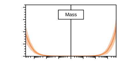
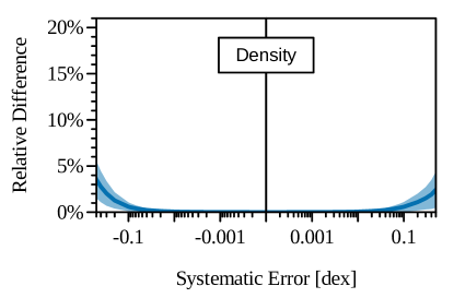
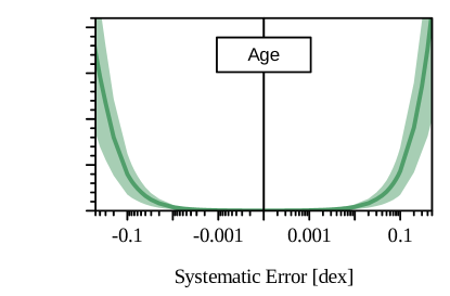
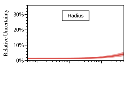
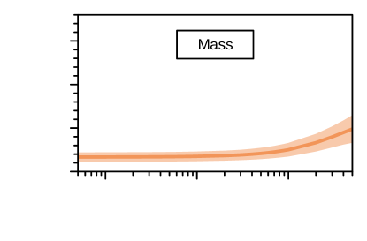
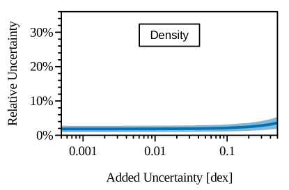
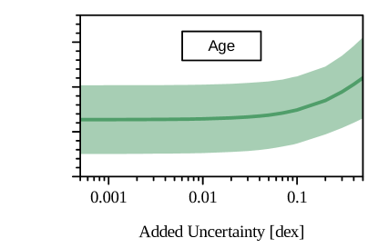
Figure 11: Average relative differences in stellar parameter estimates (radius, mass, density, and stellar age) between estimates made using the reported measurements and estimates made using [Fe/H] values that have been biased with systematic errors ranging from -0.5 dex to 0.5 dex. The lines show the mean values and the shaded regions show the standard deviations across the 97 stars.

Figure 12: Average relative uncertainties in stellar parameter estimates (radius, mass, mean density, and stellar age) as a function of the amount of additional random uncertainty given to [Fe/H] measurements ranging logarithmically from 0.0005 dex to 0.5 dex.

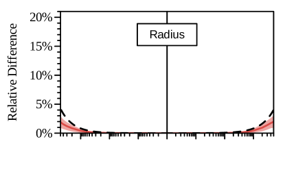
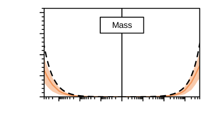
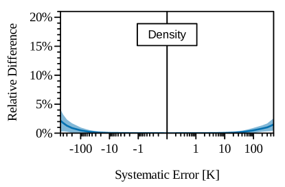
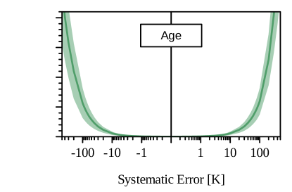
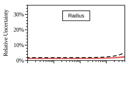
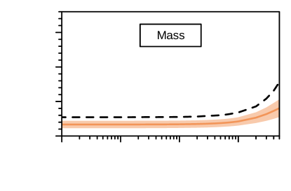
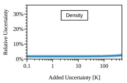
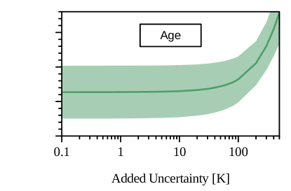
Figure 13: Average relative differences in stellar parameter estimates (radius, mass, mean density, and stellar age) between estimates made using the reported measurements and estimates made using $T_{\text{eff}}$ values that have been biased with systematic errors ranging from -500 K to 500 K. The dashed lines show the relative differences from the seismic scaling relations (Equations 1, 2 and 3).

Figure 14: Average relative uncertainties in stellar parameter estimates (radius, mass, mean density, and stellar age) as a function of the amount of additional random uncertainty given to $T_{\text{eff}}$ measurements ranging logarithmically from 0.1 K to 500 K.

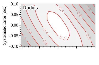
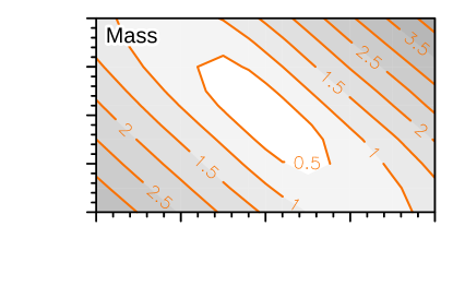
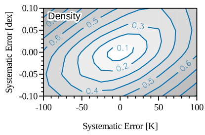
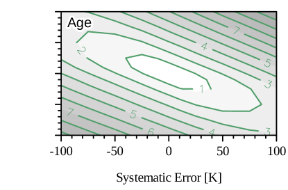
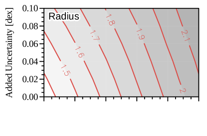
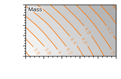
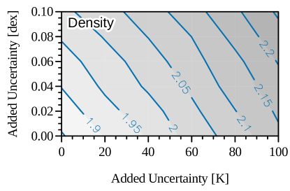
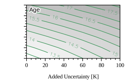
Figure 15: Average relative differences (in percent) in stellar parameter estimates (radius, mass, mean density, and stellar age) between estimates made using the reported measurements and estimates made using (simultaneously) systematically biased [Fe/H] and $T_{\text{eff}}$ values.

Figure 16: Average relative uncertainties (in percent) in stellar parameter estimates (radius, mass, mean density, and stellar age) as a function of the amount of additional random uncertainty given to [Fe/H] and $T_{\text{eff}}$ measurements.

The results of these experiments are shown in Figures 12, 12, 14, 14, 16, and 16. There it can be seen that a systematic error of 0.1 dex in [Fe/H] measurements translates on average to differences of only 4%, 2%, and 1% in the resulting stellar ages, masses, and radii, respectively. These differences are smaller than the reported relative uncertainties for these quantities ($\sim$ 11%, 3.5%, 1.4%). Similarly, a systematic error of 100 K in effective temperature results in relative differences of 6%, 2%, and 0.4%. Furthermore, increasing the reported uncertainty of [Fe/H] measurements by 0.1 dex (100%) increases the uncertainties of stellar ages, masses, and radii on average by only 0.01 Gyr, 0.02 $\text{M}_{\odot}$, and 0.01 $\text{R}_{\odot}$, which are well below the reported uncertainties for these estimates ($\sim$ 0.5 Gyr, 0.04 $\text{M}_{\odot}$, 0.02 $\text{R}_{\odot}$). Similarly, increasing the reported uncertainty of $T_{\text{eff}}$ by 100 K increases the uncertainties of the estimated stellar parameters by 0.2 Gyr, 0.01 $\text{M}_{\odot}$, and 0.003 $\text{R}_{\odot}$. Thus, even relatively large systematic errors and increases to uncertainty result in essentially the same stellar parameters.

When biasing [Fe/H] estimates by more than 0.1 dex (1$\sigma$), some of the stellar metallicities went beyond the grid of models and were dropped. By 0.5 dex (5$\sigma$), only half of the stars remained, and at this point we stopped the experiment. We find that in order for the relative differences in the resulting stellar ages, masses, and radii to be equal to their reported uncertainties, [Fe/H] ($T_{\text{eff}}$) measurements would need to be biased by at least 0.24 dex (175 K), 0.14 dex (200 K), and 0.14 dex (300 K), respectively.

The results regarding the uncertainties are consistent with the theoretical findings of Angelou et al. (2017, their Fig. 7). Though our analysis was done using frequency ratios to account for the surface term, Basu & Kinnane (2018) have similarly shown that how the surface term is accounted for does not affect estimates of the global properties (but see also Aarslev et al. 2017).

The tests regarding effective temperatures also show these biases propagated through the seismic scaling relations (Equations 1, 2, 3). We find that estimates obtained using SPI are even more robust to systematic errors than the scaling relations.

5 Conclusions

We estimated the stellar parameters of 97 main-sequence and early sub-giant stars observed by the Kepler spacecraft using the SPI pipeline. We compared the estimates of stellar mass, radius, and mean density that we obtained from stellar modeling for these stars to the estimates from seismic scaling relations and found good agreement. We found no evidence in the residuals for a trend with metallicity. We similarly compared the estimates of stellar radius and luminosity that we obtained from stellar modeling to the measurements from Gaia DR2, and again found good agreement.

We used these stars to test the impact of systematic errors in metallicity and effective temperature on the determination of stellar age, mass, and radius via asteroseismic stellar modeling. We found that the resulting stellar parameters from SPI are stable with respect to even relatively large systematic errors in the spectroscopic measurements. We emphasize that these results are only valid for asteroseismic modeling performed using SPI; results from other methods may vary. We note that we have not tested the impact on more evolved stars, such as red giants, and there too the results may differ. We note also that there may be other sources of systematic errors in the theoretical models, such as the assumed opacities, nuclear reaction rates, and mixture of metals, which we have not examined here.

These results should not be taken to imply that spectroscopic measurements are unimportant. As was shown by Bellinger et al. (2016) and Angelou et al. (2017), metallicity measurements are consistently rated as being highly important for constraining stellar models, as they provide unique information that is not redundant with the oscillation data. However, measurements of stellar metallicity are most important in constraining aspects of the models related to the initial chemical composition and mixing processes that take place during the evolution. They are, however, comparatively less important in constraining global parameters such as stellar age, mass, and radius from existing stellar models, as these quantities are well-constrained by seismology.

We conclude that asteroseismic modeling is a very reliable technique for obtaining ages, masses, radii, and other parameters of solar-like oscillators on the main sequence. Consequently, the parameters for their exoplanets, being that they are based on these values, are also robust to such systematics.

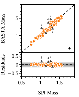
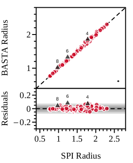
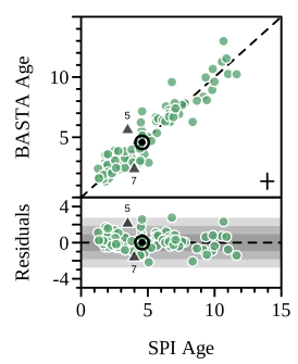
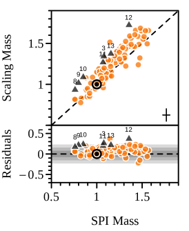
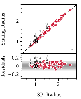
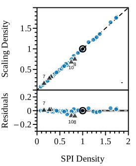
Figure 9: Comparison of stellar masses (in solar units), radii (in solar units), and ages (in Gyr) determined via stellar modeling using BASTA against those from stellar modeling using SPI. The biases in the residuals are all consistent with zero (${0.001\pm 0.061\leavevmode\nobreak\ \text{M}_{\odot}}$, ${-0.001\pm 0.027\leavevmode\nobreak\ \text{R}_{\odot}}$, and ${-0.1\pm 1.0\leavevmode\nobreak\ \text{Gyr}}$).

Figure 10: Comparison of stellar masses, radii, and mean densities (in solar units) determined via the seismic scaling relations (Equations 1, 2, 3) against those from stellar modeling using the SPI pipeline. The biases in the residuals are all consistent with zero ($0.09\pm 0.11$ $\text{M}_{\odot}$, $0.035\pm 0.045$ $\text{R}_{\odot}$, and $-0.004\pm 0.017$ $\rho_{\odot}$).

Appendix A Stellar Parameters

Table 2: Stellar parameters for the Kepler Ages and LEGACY stars from the SPI pipeline: age, mass, radius, mean density, luminosity, and number of confirmed exoplanets. The labels next to some of the KIC numbers refer to the outliers highlighted in Figure 10 and 8. The footnotes in the planets column refer to the publication that announced or confirmed their discovery.

KIC	$\tau/\text{Gyr}$	$M/\text{M}_{\odot}$	$R/\text{R}_{\odot}$	$\rho/\rho_{\odot}$	$L/\text{L}_{\odot}$	Planets
1435467	$2.03\pm 0.37$	$1.396\pm 0.033$	$1.712\pm 0.018$	$0.2789\pm 0.0045$	$4.22\pm 0.21$
2837475	$1.34\pm 0.51$	$1.455\pm 0.061$	$1.638\pm 0.022$	$0.331\pm 0.010$	$4.62\pm 0.30$
3425851	$3.77\pm 0.58$	$1.145\pm 0.049$	$1.354\pm 0.020$	$0.4625\pm 0.0062$	$2.67\pm 0.17$
3427720	$2.34\pm 0.23$	$1.108\pm 0.032$	$1.121\pm 0.010$	$0.7904\pm 0.0079$	$1.527\pm 0.079$
3456181	$2.62\pm 0.37$	$1.428\pm 0.062$	$2.125\pm 0.035$	$0.1489\pm 0.0027$	$6.79\pm 0.38$
3544595	$6.63\pm 0.64$	$0.885\pm 0.038$	$0.924\pm 0.016$	$1.128\pm 0.025$	$0.804\pm 0.058$	2
3632418	$3.40\pm 0.37$	$1.271\pm 0.047$	$1.849\pm 0.026$	$0.2008\pm 0.0020$	$4.59\pm 0.33$	1
3656476	$9.16\pm 0.80$	$1.079\pm 0.027$	$1.318\pm 0.017$	$0.4749\pm 0.0095$	$1.62\pm 0.11$
3735871	$1.81\pm 0.26$	$1.108\pm 0.032$	$1.109\pm 0.010$	$0.816\pm 0.014$	$1.535\pm 0.063$
4141376	$3.48\pm 0.56$	$0.993\pm 0.041$	$1.038\pm 0.013$	$0.897\pm 0.031$	$1.365\pm 0.094$	1
4143755	$10.56\pm 0.52$	$0.898\pm 0.019$	$1.414\pm 0.013$	$0.3211\pm 0.0036$	$1.85\pm 0.11$
4349452	$2.47\pm 0.55$	$1.206\pm 0.055$	$1.312\pm 0.023$	$0.535\pm 0.011$	$2.40\pm 0.15$	3,
4914423	$5.60\pm 0.68$	$1.117\pm 0.059$	$1.468\pm 0.021$	$0.3546\pm 0.0058$	$2.29\pm 0.14$	2
4914923	$6.37\pm 0.33$	$1.123\pm 0.033$	$1.388\pm 0.014$	$0.4207\pm 0.0042$	$2.00\pm 0.11$
5094751	$5.63\pm 0.79$	$1.072\pm 0.041$	$1.353\pm 0.019$	$0.4346\pm 0.0098$	$2.09\pm 0.13$	2
5184732	$4.84\pm 0.35$	$1.205\pm 0.022$	$1.3427\pm 0.0085$	$0.5034\pm 0.0050$	$1.912\pm 0.098$
5773345	$2.24\pm 0.50$	$1.510\pm 0.044$	$2.017\pm 0.021$	$0.1841\pm 0.0026$	$5.19\pm 0.33$
5866724	$2.53\pm 0.42$	$1.273\pm 0.032$	$1.423\pm 0.017$	$0.4434\pm 0.0064$	$2.648\pm 0.098$	3
5950854	$9.8\pm 1.1$	$0.984\pm 0.044$	$1.236\pm 0.023$	$0.524\pm 0.012$	$1.62\pm 0.14$
6106415	$4.98\pm 0.50$	$1.069\pm 0.038$	$1.219\pm 0.018$	$0.596\pm 0.011$	$1.78\pm 0.12$
6116048	$6.80\pm 0.63$	$1.002\pm 0.031$	$1.218\pm 0.014$	$0.5602\pm 0.0080$	$1.78\pm 0.11$
6196457	$4.5\pm 1.0$	$1.268\pm 0.069$	$1.756\pm 0.029$	$0.2359\pm 0.0042$	$3.29\pm 0.25$	3,
6225718${}^{\text{\hyperref@@ii[fig:scaling]{13}}}$	$3.02\pm 0.51$	$1.156\pm 0.043$	$1.234\pm 0.016$	$0.6230\pm 0.0082$	$2.19\pm 0.13$
6278762	$10.90\pm 0.86$	$0.753\pm 0.012$	$0.7588\pm 0.0045$	$1.741\pm 0.023$	$0.343\pm 0.022$	5
6508366	$2.49\pm 0.19$	$1.492\pm 0.052$	$2.177\pm 0.032$	$0.1446\pm 0.0024$	$6.91\pm 0.47$
6521045	$6.44\pm 0.35$	$1.091\pm 0.031$	$1.525\pm 0.011$	$0.3090\pm 0.0034$	$2.43\pm 0.14$	3
6603624	$7.77\pm 0.45$	$1.065\pm 0.023$	$1.173\pm 0.012$	$0.668\pm 0.016$	$1.283\pm 0.059$
6679371	$2.13\pm 0.12$	$1.570\pm 0.030$	$2.222\pm 0.017$	$0.1432\pm 0.0018$	$7.90\pm 0.44$
6933899	$6.61\pm 0.28$	$1.104\pm 0.023$	$1.599\pm 0.012$	$0.2712\pm 0.0020$	$2.67\pm 0.18$
7103006	$2.09\pm 0.45$	$1.482\pm 0.056$	$1.954\pm 0.026$	$0.1985\pm 0.0038$	$5.60\pm 0.38$
7106245${}^{\text{\hyperref@@ii[fig:scaling]{10}}}$	$8.36\pm 0.72$	$0.851\pm 0.025$	$1.048\pm 0.014$	$0.752\pm 0.017$	$1.363\pm 0.098$
7199397	$3.63\pm 0.33$	$1.308\pm 0.034$	$2.526\pm 0.028$	$0.0821\pm 0.0014$	$6.69\pm 0.29$
7206837	$1.80\pm 0.55$	$1.400\pm 0.041$	$1.584\pm 0.016$	$0.3516\pm 0.0052$	$3.58\pm 0.18$
7296438	$6.60\pm 0.40$	$1.158\pm 0.034$	$1.405\pm 0.017$	$0.4187\pm 0.0045$	$2.00\pm 0.11$
7510397${}^{\text{\hyperref@@ii[fig:scaling]{4}}}$	$3.97\pm 0.35$	$1.206\pm 0.030$	$1.784\pm 0.015$	$0.2127\pm 0.0017$	$4.18\pm 0.28$
7670943	$2.36\pm 0.47$	$1.309\pm 0.046$	$1.447\pm 0.019$	$0.4336\pm 0.0055$	$3.31\pm 0.27$
7680114	$7.57\pm 0.85$	$1.108\pm 0.033$	$1.411\pm 0.022$	$0.398\pm 0.011$	$2.07\pm 0.14$
7771282	$3.28\pm 0.56$	$1.353\pm 0.064$	$1.681\pm 0.032$	$0.2866\pm 0.0049$	$3.89\pm 0.23$
7871531	$9.34\pm 0.58$	$0.830\pm 0.022$	$0.870\pm 0.011$	$1.274\pm 0.025$	$0.632\pm 0.040$
7940546	$2.80\pm 0.20$	$1.317\pm 0.026$	$1.899\pm 0.018$	$0.1924\pm 0.0025$	$4.96\pm 0.24$
7970740	$10.67\pm 0.36$	$0.760\pm 0.014$	$0.7819\pm 0.0055$	$1.610\pm 0.013$	$0.444\pm 0.029$
8006161	$4.75\pm 0.25$	$1.004\pm 0.020$	$0.9353\pm 0.0070$	$1.233\pm 0.011$	$0.717\pm 0.040$
8077137	$4.48\pm 0.62$	$1.150\pm 0.043$	$1.638\pm 0.027$	$0.2626\pm 0.0056$	$3.37\pm 0.25$	2
8150065	$3.28\pm 0.55$	$1.196\pm 0.066$	$1.393\pm 0.032$	$0.445\pm 0.011$	$2.57\pm 0.20$
8179536	$1.84\pm 0.37$	$1.248\pm 0.059$	$1.353\pm 0.027$	$0.5039\pm 0.0081$	$2.68\pm 0.20$
8228742	$4.42\pm 0.49$	$1.221\pm 0.069$	$1.791\pm 0.041$	$0.2128\pm 0.0030$	$4.11\pm 0.36$
8292840	$2.79\pm 0.54$	$1.099\pm 0.036$	$1.321\pm 0.015$	$0.4789\pm 0.0060$	$2.40\pm 0.16$	3
8349582	$8.68\pm 0.53$	$1.144\pm 0.015$	$1.4520\pm 0.0066$	$0.3742\pm 0.0072$	$2.003\pm 0.086$	1
8379927${}^{\text{\hyperref@@ii[fig:scaling]{2}}}$	$1.84\pm 0.29$	$1.105\pm 0.049$	$1.122\pm 0.017$	$0.790\pm 0.012$	$1.55\pm 0.13$
8394589	$4.20\pm 0.39$	$1.024\pm 0.037$	$1.153\pm 0.023$	$0.673\pm 0.019$	$1.70\pm 0.11$
8424992	$10.00\pm 0.94$	$0.893\pm 0.038$	$1.033\pm 0.025$	$0.819\pm 0.027$	$1.034\pm 0.083$
8478994${}^{\text{\hyperref@@ii[fig:scaling]{9}}}$	$5.68\pm 0.96$	$0.799\pm 0.017$	$0.776\pm 0.014$	$1.732\pm 0.063$	$0.482\pm 0.032$	4,
8494142	$2.09\pm 0.32$	$1.458\pm 0.056$	$1.893\pm 0.025$	$0.2149\pm 0.0060$	$4.64\pm 0.33$	2
8554498${}^{\text{\hyperref@@ii[fig:scaling]{5}}}$	$3.49\pm 0.41$	$1.320\pm 0.026$	$1.840\pm 0.017$	$0.2126\pm 0.0030$	$3.86\pm 0.17$
8684730	$2.55\pm 0.45$	$1.475\pm 0.039$	$2.105\pm 0.039$	$0.163\pm 0.011$	$5.01\pm 0.25$
8694723${}^{\text{\hyperref@@ii[fig:scaling]{11}}}$	$5.26\pm 0.23$	$1.070\pm 0.023$	$1.515\pm 0.013$	$0.3084\pm 0.0039$	$3.16\pm 0.19$
8760414${}^{\text{\hyperref@@ii[fig:scaling]{8}}}$	$15.78\pm 0.91$	$0.761\pm 0.011$	$0.9755\pm 0.0090$	$0.828\pm 0.015$	$1.032\pm 0.064$
8866102	$1.81\pm 0.27$	$1.223\pm 0.054$	$1.357\pm 0.022$	$0.4902\pm 0.0048$	$2.66\pm 0.16$
8938364	$11.02\pm 0.58$	$0.995\pm 0.023$	$1.363\pm 0.011$	$0.3955\pm 0.0046$	$1.74\pm 0.10$
9025370${}^{\text{\hyperref@@ii[fig:scaling]{1}}}$	$5.77\pm 0.60$	$0.921\pm 0.035$	$0.987\pm 0.019$	$0.965\pm 0.019$	$0.709\pm 0.084$
9098294	$9.42\pm 0.85$	$0.934\pm 0.041$	$1.112\pm 0.027$	$0.682\pm 0.021$	$1.301\pm 0.081$
9139151	$1.82\pm 0.19$	$1.205\pm 0.044$	$1.168\pm 0.016$	$0.7566\pm 0.0097$	$1.96\pm 0.12$
9139163	$2.09\pm 0.28$	$1.378\pm 0.039$	$1.557\pm 0.017$	$0.3653\pm 0.0038$	$3.70\pm 0.22$
9206432${}^{\text{\hyperref@@ii[fig:scaling]{12}}}$	$1.67\pm 0.42$	$1.355\pm 0.047$	$1.505\pm 0.021$	$0.3982\pm 0.0065$	$3.76\pm 0.21$
9353712	$2.44\pm 0.21$	$1.465\pm 0.054$	$2.164\pm 0.032$	$0.1446\pm 0.0019$	$6.60\pm 0.50$
9410862	$7.34\pm 0.75$	$0.954\pm 0.028$	$1.139\pm 0.017$	$0.650\pm 0.019$	$1.580\pm 0.099$
9414417	$2.80\pm 0.22$	$1.319\pm 0.041$	$1.882\pm 0.023$	$0.1978\pm 0.0026$	$4.89\pm 0.29$
9592705	$2.21\pm 0.19$	$1.521\pm 0.044$	$2.118\pm 0.026$	$0.1610\pm 0.0036$	$5.94\pm 0.37$
9812850	$1.99\pm 0.39$	$1.417\pm 0.057$	$1.805\pm 0.025$	$0.2399\pm 0.0067$	$4.71\pm 0.24$
9955598	$6.69\pm 0.48$	$0.921\pm 0.032$	$0.893\pm 0.012$	$1.306\pm 0.015$	$0.634\pm 0.042$	1
9965715${}^{\text{\hyperref@@ii[fig:scaling]{6}}}$	$3.88\pm 0.49$	$1.030\pm 0.023$	$1.244\pm 0.011$	$0.538\pm 0.013$	$1.78\pm 0.17$
10068307${}^{\text{\hyperref@@ii[fig:scaling]{7}}}$	$3.98\pm 0.34$	$1.271\pm 0.045$	$2.024\pm 0.023$	$0.1546\pm 0.0015$	$5.24\pm 0.37$
10079226	$2.56\pm 0.40$	$1.153\pm 0.050$	$1.160\pm 0.016$	$0.744\pm 0.013$	$1.521\pm 0.088$
10162436	$3.29\pm 0.42$	$1.379\pm 0.052$	$2.019\pm 0.026$	$0.1678\pm 0.0017$	$5.25\pm 0.31$
10454113${}^{\text{\hyperref@@ii[fig:scaling]{3}}}$	$5.07\pm 0.91$	$1.078\pm 0.048$	$1.202\pm 0.022$	$0.659\pm 0.018$	$1.94\pm 0.13$
10514430	$7.01\pm 0.61$	$1.042\pm 0.029$	$1.578\pm 0.016$	$0.2664\pm 0.0034$	$2.55\pm 0.16$
10516096	$6.66\pm 0.47$	$1.108\pm 0.035$	$1.422\pm 0.017$	$0.3861\pm 0.0029$	$2.30\pm 0.17$
10586004	$6.13\pm 0.89$	$1.154\pm 0.041$	$1.643\pm 0.029$	$0.2605\pm 0.0056$	$2.73\pm 0.20$	2
10644253	$1.28\pm 0.25$	$1.128\pm 0.027$	$1.1204\pm 0.0085$	$0.804\pm 0.012$	$1.525\pm 0.060$
10666592	$2.02\pm 0.25$	$1.556\pm 0.046$	$2.009\pm 0.023$	$0.1918\pm 0.0027$	$5.92\pm 0.42$	1
10730618	$4.4\pm 1.1$	$1.249\pm 0.085$	$1.716\pm 0.053$	$0.251\pm 0.012$	$3.81\pm 0.52$
10963065	$4.57\pm 0.48$	$1.065\pm 0.043$	$1.225\pm 0.026$	$0.584\pm 0.017$	$1.93\pm 0.13$	1
11081729	$1.66\pm 0.84$	$1.363\pm 0.039$	$1.444\pm 0.018$	$0.4526\pm 0.0082$	$3.46\pm 0.20$
11133306	$4.58\pm 0.74$	$1.081\pm 0.040$	$1.198\pm 0.016$	$0.634\pm 0.015$	$1.66\pm 0.11$
11253226	$1.34\pm 0.50$	$1.420\pm 0.071$	$1.599\pm 0.026$	$0.3468\pm 0.0094$	$4.53\pm 0.29$
11295426	$6.31\pm 0.39$	$1.099\pm 0.031$	$1.251\pm 0.013$	$0.5673\pm 0.0080$	$1.587\pm 0.096$	3
11401755	$6.94\pm 0.78$	$1.043\pm 0.031$	$1.601\pm 0.026$	$0.2552\pm 0.0074$	$2.91\pm 0.21$	2
11772920	$9.9\pm 1.1$	$0.823\pm 0.040$	$0.845\pm 0.018$	$1.373\pm 0.024$	$0.468\pm 0.068$
11807274	$2.01\pm 0.28$	$1.306\pm 0.032$	$1.597\pm 0.013$	$0.3223\pm 0.0052$	$3.51\pm 0.17$	2
11853905	$6.60\pm 0.57$	$1.163\pm 0.046$	$1.588\pm 0.019$	$0.2911\pm 0.0042$	$2.53\pm 0.17$	1
11904151	$11.65\pm 0.93$	$0.880\pm 0.031$	$1.041\pm 0.016$	$0.784\pm 0.022$	$0.995\pm 0.054$	2,
12009504	$3.80\pm 0.29$	$1.197\pm 0.044$	$1.411\pm 0.018$	$0.4266\pm 0.0054$	$2.63\pm 0.16$
12069127	$2.31\pm 0.18$	$1.537\pm 0.051$	$2.297\pm 0.030$	$0.1267\pm 0.0015$	$7.48\pm 0.44$
12069424	$6.92\pm 0.25$	$1.056\pm 0.019$	$1.213\pm 0.011$	$0.5967\pm 0.0085$	$1.531\pm 0.076$
12069449	$7.08\pm 0.22$	$1.0000\pm 0.0086$	$1.101\pm 0.012$	$0.758\pm 0.018$	$1.201\pm 0.024$	1
12258514	$4.40\pm 0.29$	$1.252\pm 0.054$	$1.614\pm 0.023$	$0.2999\pm 0.0024$	$2.95\pm 0.18$
12317678	$2.63\pm 0.28$	$1.288\pm 0.036$	$1.775\pm 0.022$	$0.2301\pm 0.0042$	$5.33\pm 0.25$

References

- Aarslev et al. (2017) Aarslev, M. J., Christensen-Dalsgaard, J., Lund, M. N., Silva Aguirre, V., & Gough, D. 2017, in European Physical Journal Web of Conferences, Vol. 160, European Physical Journal Web of Conferences, 03010
- Adibekyan et al. (2018) Adibekyan, V., Sousa, S. G., & Santos, N. C. 2018, Asteroseismology and Exoplanets: Listening to the Stars and Searching for New Worlds, 49, 225
- Akeson et al. (2013) Akeson, R. L., Chen, X., Ciardi, D., et al. 2013, PASP, 125, 989
- Anders et al. (2017) Anders, F., Chiappini, C., Rodrigues, T. S., et al. 2017, A&A, 597, A30
- Andrae et al. (2018) Andrae, R., Fouesneau, M., Creevey, O., et al. 2018, A&A, 616, A8
- Angelou et al. (2017) Angelou, G. C., Bellinger, E. P., Hekker, S., & Basu, S. 2017, ApJ, 839, 116
- Barclay et al. (2013) Barclay, T., Rowe, J. F., Lissauer, J. J., et al. 2013, Nature, 494, 452
- Basu (1997) Basu, S. 1997, MNRAS, 288, 572
- Basu & Chaplin (2017) Basu, S. & Chaplin, W. 2017, Asteroseismic Data Analysis: Foundations and Techniques, Princeton Series in Modern Obs (Princeton University Press)
- Basu & Kinnane (2018) Basu, S. & Kinnane, A. 2018, ArXiv e-prints [arXiv:1810.07205]
- Batalha et al. (2011) Batalha, N. M., Borucki, W. J., Bryson, S. T., et al. 2011, ApJ, 729, 27
- Belkacem et al. (2011) Belkacem, K., Goupil, M. J., Dupret, M. A., et al. 2011, A&A, 530, A142
- Bellinger et al. (2016) Bellinger, E. P., Angelou, G. C., Hekker, S., et al. 2016, ApJ, 830, 31
- Bellinger et al. (2017) Bellinger, E. P., Basu, S., Hekker, S., & Ball, W. H. 2017, ApJ, 851, 80
- Borucki et al. (2010a) Borucki, W. J., Koch, D., Basri, G., et al. 2010a, Science, 327, 977
- Borucki et al. (2010b) Borucki, W. J., Koch, D. G., Brown, T. M., et al. 2010b, ApJ, 713, L126
- Breiman (2001) Breiman, L. 2001, Machine Learning, 45, 5
- Brown et al. (1994) Brown, T. M., Christensen-Dalsgaard, J., Weibel-Mihalas, B., & Gilliland, R. L. 1994, ApJ, 427, 1013
- Brown et al. (1991) Brown, T. M., Gilliland, R. L., Noyes, R. W., & Ramsey, L. W. 1991, ApJ, 368, 599
- Campante et al. (2015) Campante, T. L., Barclay, T., Swift, J. J., et al. 2015, ApJ, 799, 170
- Campante et al. (2016) Campante, T. L., Lund, M. N., Kuszlewicz, J. S., et al. 2016, ApJ, 819, 85
- Carter et al. (2012) Carter, J. A., Agol, E., Chaplin, W. J., et al. 2012, Science, 337, 556
- Chaplin & Miglio (2013) Chaplin, W. J. & Miglio, A. 2013, ARA&A, 51, 353
- Chaplin et al. (2013) Chaplin, W. J., Sanchis-Ojeda, R., Campante, T. L., et al. 2013, ApJ, 766, 101
- Chiappini et al. (2015) Chiappini, C., Anders, F., Rodrigues, T. S., et al. 2015, A&A, 576, L12
- Christensen-Dalsgaard (1984) Christensen-Dalsgaard, J. 1984, in Space Research in Stellar Activity and Variability, ed. A. Mangeney & F. Praderie, 11
- Christensen-Dalsgaard & Silva Aguirre (2018) Christensen-Dalsgaard, J. & Silva Aguirre, V. 2018, in Handbook of Exoplanets, ed. Deeg, Hans J. and Belmonte, Juan Antonio (Springer), 18
- Cochran et al. (1997) Cochran, W. D., Hatzes, A. P., Butler, R. P., & Marcy, G. W. 1997, ApJ, 483, 457
- Creevey et al. (2013) Creevey, O. L., Thévenin, F., Basu, S., et al. 2013, MNRAS, 431, 2419
- Davies et al. (2016) Davies, G. R., Silva Aguirre, V., Bedding, T. R., et al. 2016, MNRAS, 456, 2183
- Deheuvels et al. (2016) Deheuvels, S., Brandão, I., Silva Aguirre, V., et al. 2016, A&A, 589, A93
- Feuillet et al. (2018) Feuillet, D. K., Bovy, J., Holtzman, J., et al. 2018, MNRAS, 477, 2326
- Fressin et al. (2011) Fressin, F., Torres, G., Désert, J.-M., et al. 2011, ApJS, 197, 5
- Friedman et al. (2001) Friedman, J., Hastie, T., & Tibshirani, R. 2001, The Elements of Statistical Learning, Vol. 1 (Springer New York)
- Gai et al. (2011) Gai, N., Basu, S., Chaplin, W. J., & Elsworth, Y. 2011, ApJ, 730, 63
- Gaia Collaboration et al. (2018) Gaia Collaboration, Brown, A. G. A., Vallenari, A., et al. 2018, A&A, 616, A1
- Gaulme et al. (2016) Gaulme, P., McKeever, J., Jackiewicz, J., et al. 2016, ApJ, 832, 121
- Geurts et al. (2006) Geurts, P., Ernst, D., & Wehenkel, L. 2006, Machine Learning, 63, 3
- Gilliland et al. (2013) Gilliland, R. L., Marcy, G. W., Rowe, J. F., et al. 2013, ApJ, 766, 40
- Ginsburg et al. (2018) Ginsburg, A., Sipocz, B., Parikh, M., et al. 2018, astropy/astroquery: v0.3.7 release
- Gratia & Fabrycky (2017) Gratia, P. & Fabrycky, D. 2017, MNRAS, 464, 1709
- Guggenberger et al. (2017) Guggenberger, E., Hekker, S., Angelou, G. C., Basu, S., & Bellinger, E. P. 2017, MNRAS, 470, 2069
- Guggenberger et al. (2016) Guggenberger, E., Hekker, S., Basu, S., & Bellinger, E. 2016, MNRAS, 460, 4277
- Guillochon et al. (2011) Guillochon, J., Ramirez-Ruiz, E., & Lin, D. 2011, ApJ, 732, 74
- Hadden & Lithwick (2014) Hadden, S. & Lithwick, Y. 2014, ApJ, 787, 80
- Han et al. (2014) Han, E., Wang, S. X., Wright, J. T., et al. 2014, PASP, 126, 827
- Haywood et al. (2018) Haywood, R. D., Vanderburg, A., Mortier, A., et al. 2018, AJ, 155, 203
- Hekker et al. (2013) Hekker, S., Elsworth, Y., Mosser, B., et al. 2013, A&A, 556, A59
- Hjørringgaard et al. (2017) Hjørringgaard, J. G., Silva Aguirre, V., White, T. R., et al. 2017, MNRAS, 464, 3713
- Howell et al. (2012) Howell, S. B., Rowe, J. F., Bryson, S. T., et al. 2012, ApJ, 746, 123
- Huber (2016) Huber, D. 2016, IAU Focus Meeting, 29, 620
- Huber (2018) Huber, D. 2018, Asteroseismology and Exoplanets: Listening to the Stars and Searching for New Worlds, 49, 119
- Huber et al. (2011) Huber, D., Bedding, T. R., Stello, D., et al. 2011, ApJ, 743, 143
- Huber et al. (2013) Huber, D., Carter, J. A., Barbieri, M., et al. 2013, Science, 342, 331
- Huber et al. (2014) Huber, D., Silva Aguirre, V., Matthews, J. M., et al. 2014, ApJS, 211, 2
- Huber et al. (2017) Huber, D., Zinn, J., Bojsen-Hansen, M., et al. 2017, ApJ, 844, 102
- Jenkins et al. (2015) Jenkins, J. M., Twicken, J. D., Batalha, N. M., et al. 2015, AJ, 150, 56
- Kamiaka et al. (2018) Kamiaka, S., Benomar, O., & Suto, Y. 2018, MNRAS, 479, 391
- Kjeldsen & Bedding (1995) Kjeldsen, H. & Bedding, T. R. 1995, A&A, 293, 87
- Königl et al. (2017) Königl, A., Giacalone, S., & Matsakos, T. 2017, ApJ, 846, L13
- Lai et al. (2011) Lai, D., Foucart, F., & Lin, D. N. C. 2011, MNRAS, 412, 2790
- Lebreton & Goupil (2014) Lebreton, Y. & Goupil, M. J. 2014, A&A, 569, A21
- Li & Winn (2016) Li, G. & Winn, J. N. 2016, ApJ, 818, 5
- Lin et al. (1996) Lin, D. N. C., Bodenheimer, P., & Richardson, D. C. 1996, Nature, 380, 606
- Lund et al. (2017) Lund, M. N., Silva Aguirre, V., Davies, G. R., et al. 2017, ApJ, 835, 172
- Lundkvist et al. (2018) Lundkvist, M. S., Huber, D., Silva Aguirre, V., & Chaplin, W. J. 2018, in Handbook of Exoplanets, ed. Deeg, Hans J. and Belmonte, Juan Antonio (Springer), 24
- Marcy et al. (2014) Marcy, G. W., Isaacson, H., Howard, A. W., et al. 2014, ApJS, 210, 20
- Marrese et al. (2018) Marrese, P. M., Marinoni, S., Fabrizio, M., & Altavilla, G. 2018, ArXiv e-prints [arXiv:1808.09151]
- Massey & Hanson (2013) Massey, P. & Hanson, M. M. 2013, Astronomical Spectroscopy (Springer), 35
- Mathur et al. (2012) Mathur, S., Metcalfe, T. S., Woitaszek, M., et al. 2012, ApJ, 749, 152
- Matsakos & Königl (2015) Matsakos, T. & Königl, A. 2015, ApJ, 809, L20
- Matsakos & Königl (2017) Matsakos, T. & Königl, A. 2017, AJ, 153, 60
- Metcalfe et al. (2014) Metcalfe, T. S., Creevey, O. L., Doğan, G., et al. 2014, ApJS, 214, 27
- Morton & Johnson (2011) Morton, T. D. & Johnson, J. A. 2011, ApJ, 729, 138
- Mosser et al. (2013) Mosser, B., Michel, E., Belkacem, K., et al. 2013, A&A, 550, A126
- Nissen et al. (2017) Nissen, P. E., Silva Aguirre, V., Christensen-Dalsgaard, J., et al. 2017, A&A, 608, A112
- Pál et al. (2008) Pál, A., Bakos, G. Á., Torres, G., et al. 2008, ApJ, 680, 1450
- Paxton et al. (2011) Paxton, B., Bildsten, L., Dotter, A., et al. 2011, ApJS, 192, 3
- Paxton et al. (2013) Paxton, B., Cantiello, M., Arras, P., et al. 2013, ApJS, 208, 4
- Paxton et al. (2015) Paxton, B., Marchant, P., Schwab, J., et al. 2015, ApJS, 220, 15
- Paxton et al. (2018) Paxton, B., Schwab, J., Bauer, E. B., et al. 2018, ApJS, 234, 34
- Plavchan & Bilinski (2013) Plavchan, P. & Bilinski, C. 2013, ApJ, 769, 86
- Prša et al. (2016) Prša, A., Harmanec, P., Torres, G., et al. 2016, AJ, 152, 41
- Rogers (2015) Rogers, L. A. 2015, ApJ, 801, 41
- Rowe et al. (2014) Rowe, J. F., Bryson, S. T., Marcy, G. W., et al. 2014, ApJ, 784, 45
- Roxburgh & Vorontsov (2003) Roxburgh, I. W. & Vorontsov, S. V. 2003, A&A, 411, 215
- Safonova et al. (2016) Safonova, M., Murthy, J., & Shchekinov, Y. A. 2016, International Journal of Astrobiology, 15, 93
- Sahlholdt & Silva Aguirre (2018) Sahlholdt, C. L. & Silva Aguirre, V. 2018, MNRAS, 481, L125
- Seager et al. (2007) Seager, S., Kuchner, M., Hier-Majumder, C. A., & Militzer, B. 2007, ApJ, 669, 1279
- Seager & Mallén-Ornelas (2003) Seager, S. & Mallén-Ornelas, G. 2003, ApJ, 585, 1038
- Sharma et al. (2016) Sharma, S., Stello, D., Bland-Hawthorn, J., Huber, D., & Bedding, T. R. 2016, ApJ, 822, 15
- Silva Aguirre et al. (2018) Silva Aguirre, V., Bojsen-Hansen, M., Slumstrup, D., et al. 2018, MNRAS, 475, 5487
- Silva Aguirre et al. (2015) Silva Aguirre, V., Davies, G. R., Basu, S., et al. 2015, MNRAS, 452, 2127
- Silva Aguirre et al. (2017) Silva Aguirre, V., Lund, M. N., Antia, H. M., et al. 2017, ApJ, 835, 173
- Steffen et al. (2013) Steffen, J. H., Fabrycky, D. C., Agol, E., et al. 2013, MNRAS, 428, 1077
- Steffen et al. (2012) Steffen, J. H., Fabrycky, D. C., Ford, E. B., et al. 2012, MNRAS, 421, 2342
- Teyssandier et al. (2013) Teyssandier, J., Terquem, C., & Papaloizou, J. C. B. 2013, MNRAS, 428, 658
- Themeßl et al. (2018) Themeßl, N., Hekker, S., Southworth, J., et al. 2018, MNRAS, 478, 4669
- Thies et al. (2011) Thies, I., Kroupa, P., Goodwin, S. P., Stamatellos, D., & Whitworth, A. P. 2011, MNRAS, 417, 1817
- Torres et al. (2010) Torres, G., Andersen, J., & Giménez, A. 2010, A&A Rev., 18, 67
- Townsend & Teitler (2013) Townsend, R. H. D. & Teitler, S. A. 2013, MNRAS, 435, 3406
- Ulrich (1986) Ulrich, R. K. 1986, ApJ, 306, L37
- Škoda (2017) Škoda, P. 2017, in Proceedings of EURO-VO Workshop Astronomical Spectroscopy and Virtual Observatory
- Valle et al. (2018) Valle, G., Dell’Omodarme, M., Prada Moroni, P. G., & Degl’Innocenti, S. 2018, ArXiv e-prints [arXiv:1810.06997]
- Van Eylen & Albrecht (2015) Van Eylen, V. & Albrecht, S. 2015, ApJ, 808, 126
- Van Eylen et al. (2014) Van Eylen, V., Lund, M. N., Silva Aguirre, V., et al. 2014, ApJ, 782, 14
- Viani et al. (2017) Viani, L. S., Basu, S., Chaplin, W. J., Davies, G. R., & Elsworth, Y. 2017, ApJ, 843, 11
- Watson et al. (2011) Watson, C. A., Littlefair, S. P., Diamond, C., et al. 2011, MNRAS, 413, L71
- Weiss & Marcy (2014) Weiss, L. M. & Marcy, G. W. 2014, ApJ, 783, L6
- White et al. (2011) White, T. R., Bedding, T. R., Stello, D., et al. 2011, ApJ, 743, 161
- Xie (2014) Xie, J.-W. 2014, ApJS, 210, 25