Computing the Hausdorff Distance of Two Sets from Their Signed Distance Functions

Abstract

The Hausdorff distance is a measure of (dis-)similarity between two sets which is widely used in various applications. Most of the applied literature is devoted to the computation for sets consisting of a finite number of points. This has applications, for instance, in image processing. However, we would like to apply the Hausdorff distance to control and evaluate optimisation methods in level-set based shape optimisation. In this context, the involved sets are not finite point sets but characterised by level-set or signed distance functions. This paper discusses the computation of the Hausdorff distance between two such sets. We recall fundamental properties of the Hausdorff distance, including a characterisation in terms of distance functions. In numerical applications, this result gives at least an exact lower bound on the Hausdorff distance. We also derive an upper bound, and consequently a precise error estimate. By giving an example, we show that our error estimate cannot be further improved for a general situation. On the other hand, we also show that much better accuracy can be expected for non-pathological situations that are more likely to occur in practice. The resulting error estimate can be improved even further if one assumes that the grid is rotated randomly with respect to the involved sets.

Keywords: Hausdorff Distance, Signed Distance Function, Level-Set Method, Error Estimate, Stochastic Error Analysis

1 Introduction

The Hausdorff distance (also called Pompeiu-Hausdorff distance) is a classical measure for the difference between two sets:

Definition 1.

Let $A,B\subset\mathbb{R}^{n}$. Then the one-sided Hausdorff distance between $A$ and $B$ is defined as

$$d\left(A\to B\right)=\sup_{x\in A}\inf_{y\in B}\left|x-y\right|.$$ (1)

This allows us to introduce the Hausdorff distance:

$$d_{H}(A,B)=\max\left(d\left(A\to B\right),\,d\left(B\to A\right)\right)$$ (2)

While one can, in fact, define the Hausdorff distance between subsets of a general metric space, we are only interested in subsets of $\mathbb{R}^{n}$ in the following. Note that $d\left(A\to B\right)\neq d\left(B\to A\right)$ in general, such that the additional symmetrisation step in (2) is necessary. For instance, if $A\subset B$, then $d\left(A\to B\right)=0$ while $d_{H}(A,B)=d\left(B\to A\right)>0$ unless $\overline{A}=\overline{B}$. Since the Euclidean norm $\left|\cdot\right|$ is continuous, it is easy to see that (1) and thus also $d_{H}$ is not changed if we replace one or both of the sets by their interior or closure. The set of compact subsets of $\mathbb{R}^{n}$ is turned into a metric space by $d_{H}$. For some general discussion about the Hausdorff distance, see Subsection 6.2.2 of [3]. The main theoretical properties that we need will be discussed in Section 2 in more detail.

Historically, the Hausdorff distance is a relatively old concept. It was already introduced by Hausdorff in 1914, with a similar concept for the reciprocal distance between two sets dating back to Pompeiu in 1905. In recent decades, the Hausdorff distance has found plenty of applications in various fields. For instance, it has been applied in image processing [6], object matching [16], face detection [7] and for evolutionary optimisation [14], to name just a few selected areas. In most of these applications, the sets whose distance is computed are finite point sets. Those sets may come, for instance, from filtering a digital image or a related process. Consequently, there exists a lot of literature that deals with the computation of the Hausdorff distance for point sets, such as [11]. Methods exist also for sets of other structure, for instance, convex polygons [1].

We are specifically interested in applying the Hausdorff distance to measure and control the progress of level-set based shape optimisation algorithms such as the methods employed in [8] and [9]. In particular, the Hausdorff distance between successive iterates produced by some descent method may be useful to implement a stopping criterion or to detect when a descent run is getting stuck in a local minimum. For these applications, the sets $A$ and $B$ are typically open domains that are described by the sub-zero level sets of some functions. To the best of our knowledge, no analysis has been done so far on the computation of the Hausdorff distance for sets given in this way. A special choice for the level-set function of a domain is its signed distance function:

Definition 2.

Let $\Omega\subset\mathbb{R}^{n}$ be bounded. We define the distance function of $\Omega$ as

$$d_{\Omega}(x)=\inf_{y\in\Omega}\left|x-y\right|.$$

Note that $d_{\Omega}(x)=0$ for all $x\in\overline{\Omega}$. To capture also information about the interior of $\Omega$, we introduce the signed (or oriented) distance function as well:

$$\mathrm{sd}_{\Omega}(x)=\left\{\begin{array}[]{rl}d_{\Omega}(x)&x\not\in\Omega,\\ -d_{\mathbb{R}^{n}\setminus\Omega}(x)&x\in\Omega\\ \end{array}\right.$$

See also chapters 6 and 7 of [3]. Both $d_{\Omega}$ and $\mathrm{sd}_{\Omega}$ are Lipschitz continuous with constant one.

If the signed distance function of $\Omega$ is not known, it can be calculated very efficiently from an arbitrary level-set function using the Fast Marching Method [15]. Conveniently, the Hausdorff distance can be characterised in terms of distance functions. It should not come as a big surprise that this is possible, considering that the distance function $d_{B}(x)$ appears on the right-hand side of (1). This is a classical result, which we will recall and discuss in Section 2. For numerical calculations, though, the distance functions are known only on a finite number of grid points. In this case, the classical characterisation only yields an exact lower bound for $d_{H}(A,B)$. The main result of this paper is the derivation of upper bounds as well, such that the approximation error can be estimated. These results will be presented in Section 3. We also give an example to show that our estimates of Subsection 3.1 are sharp in the general case. In addition, we will see that much better estimates can be achieved for (a little) more specific situations. Since these situations still cover a wide range of sets that may occur in practical applications, this result is also useful. Subsection 3.3 gives a comparison of the actual numerical error for some situations in which $d_{H}(A,B)$ is known exactly. We will see that these results match the theoretical conclusions quite well. In Section 4, finally, we show that further improvements are possible if we assume that the orientation of the grid is not related to the sets $A$ and $B$. This can be achieved, for instance, by a random rotation of the grid, and is usually justified if the data comes from a measurement process.

Note that our code for the computation of (signed) distance functions as well as the Hausdorff distance following the method suggested here has been released as free software. It is included in the level-set package [10] for GNU Octave [5].

2 Characterising $d_{H}$ in Terms of Distance Functions

Let $A,B\subset\mathbb{R}^{n}$ be two compact sets throughout the remainder of the paper. In this case, it is easy to see that compactness implies that the various suprema and infima in Definition 1 and Definition 2 are actually attained:

Lemma 1.

For each $x\in\mathbb{R}^{n}$ there exist $y_{1},y_{2}\in A$ such that $d_{A}(x)=\left|x-y_{1}\right|$ and $\left|\mathrm{sd}_{A}(x)\right|=\left|x-y_{2}\right|$. Furthermore, there also exist $x\in A$ and $y\in B$ such that $d\left(A\to B\right)=\left|x-y\right|$. This, of course, implies that $d_{H}(A,B)$ can also be expressed in a similar form.

Let us now, for the rest of this section, turn our attention to the relation between the Hausdorff distance and distance functions. While most of this content is well-known and not new, we believe that it makes sense to give a comprehensive discussion. This is particularly true because the Hausdorff distance is a concept that can be quite unintuitive. Thus, we try to clearly explain potential pitfalls and give counterexamples where appropriate. This discussion forms the basis for the later sections, in which we present our new results.

2.1 Distance Functions

One may have the idea to “characterise” the sets $A$ and $B$ via their distance functions $d_{A}$ and $d_{B}$ from Definition 2. Since the distance functions are part of the Banach space $C(\mathbb{R}^{n})$ of continuous functions, the norm on this space can be used to define a distance between $A$ and $B$ as $\left\|d_{A}-d_{B}\right\|_{\infty}$. We will now see that this distance is equal to the Hausdorff distance defined in Definition 1:

Theorem 1.

For each $x\in\mathbb{R}^{n}$, the inequality

$$\left|d_{A}(x)-d_{B}(x)\right|\leq d_{H}(A,B)$$ (3)

holds. More precisely, one even has

$$d_{H}(A,B)=\left\|d_{A}-d_{B}\right\|_{\infty}=\sup_{x\in\mathbb{R}^{n}}\left|d_{A}(x)-d_{B}(x)\right|.$$ (4)

Proof.

This is a classical result, which is, for instance, given also on page 270 of [3]. Since the argumentation there contains a small gap, we provide a proof here nevertheless for convenience.

Assume first that $x\in A$. In this case, $d_{A}(x)=0$ such that $\left|d_{A}(x)-d_{B}(x)\right|=d_{B}(x)$. Since

$$d_{H}(A,B)\geq d\left(A\to B\right)=\sup_{y\in A}d_{B}(y)\geq d_{B}(x),$$

the estimate (3) follows. A similar argument can be applied if $x\in B$. Thus, it remains to consider the case $x\in\mathbb{R}^{n}\setminus(A\cup B)$. According to Lemma 1, we can choose $y\in B$ with $d_{B}(x)=\left|x-y\right|$. There also exists $z\in A$ such that $d_{A}(y)=\left|z-y\right|$. Then (3) follows, since

$$d_{A}(x)-d_{B}(x)\leq\left|x-z\right|-\left|x-y\right|\leq\left|z-y\right|=d_{A}(y)\leq d\left(B\to A\right)\leq d_{H}(A,B).$$

To show also (4), let us assume, without loss of generality, that $d_{H}(A,B)=d\left(A\to B\right)$. But since

$$d\left(A\to B\right)=\sup_{x\in A}d_{B}(x)=\sup_{x\in A}\left|d_{A}(x)-d_{B}(x)\right|\leq\left\|d_{A}-d_{B}\right\|_{\infty},$$ (5)

the claim follows. ∎

Theorem 1 forms the foundation for the remainder of our paper: It gives a representation of the Hausdorff distance in terms of the distance functions. Furthermore, it is also easy to actually evaluate this representation in practice. In particular, if $d_{A}$ and $d_{B}$ are given numerically on a grid, one can just consider $\left|d_{A}(x_{i})-d_{B}(x_{i})\right|$ for all grid points $x_{i}$. The largest difference obtained in this way is guaranteed to be at least a lower bound for $d_{H}(A,B)$. If the maximising point for (4) is not a grid point, however, we can not expect to get equality with the Hausdorff distance. Section 3 will be devoted to a discussion of the possible error introduced in this way.

It is sometimes convenient to use not the Hausdorff distance itself, but the so-called complementary Hausdorff distance $d_{H}(\mathbb{R}^{n}\setminus A,\,\mathbb{R}^{n}\setminus B)$ instead. (Particularly when dealing with open domains in applications.) See, for instance, [2]. In this case, our assumption of compact sets is not fulfilled any more, since the complements are unbounded if the sets themselves are bounded. However, one can verify that Lemma 1 and Theorem 1 are still valid also for this situation.

2.2 Signed Distances

We turn our focus now to signed distance functions: Since $\mathrm{sd}_{A}$ and $\mathrm{sd}_{B}$ are in $C(\mathbb{R}^{n})$ as well, also $\left\|\mathrm{sd}_{A}-\mathrm{sd}_{B}\right\|_{\infty}$ can be used as a distance measure between $A$ and $B$. See also Subsection 7.2.2 of [3]. This distance is, however, not equal to $d_{H}(A,B)$:

Example 1.

Let $0<r<R$ be given, and define $A=\overline{B_{R}\left(0\right)}$, $B=A\setminus B_{r}\left(0\right)$. This situation is depicted in Figure 1. Then $d_{H}(A,B)=d\left(A\to B\right)=r$, as highlighted in the sketch with the red line. On the other hand, $\mathrm{sd}_{A}(0)=-R$ while $\mathrm{sd}_{B}(0)=r$. Hence,

$$\left\|\mathrm{sd}_{A}-\mathrm{sd}_{B}\right\|_{\infty}\geq\left|\mathrm{sd}_{A}(0)-\mathrm{sd}_{B}(0)\right|=R+r>r=d_{H}(A,B).$$

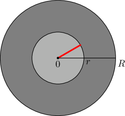
Figure 1: Sketch for the situation of Example 1. The dark ring is $B=A\cap B$, while the inner circle is $A\setminus B$. The red line shows the Hausdorff distance between $A$ and $B$.

In fact, one can show that $\left\|\mathrm{sd}_{A}-\mathrm{sd}_{B}\right\|_{\infty}$ induces a stronger metric between the sets than either the complementary or the ordinary Hausdorff distance alone:

Theorem 2.

Let $x\in\mathbb{R}^{n}$. Then

$$\left|\mathrm{sd}_{A}(x)-\mathrm{sd}_{B}(x)\right|=\left|d_{A}(x)-d_{B}(x)\right|+\left|d_{\mathbb{R}^{n}\setminus A}(x)-d_{\mathbb{R}^{n}\setminus B}(x)\right|.$$ (6)

Consequently, also

$$\max\left(d_{H}(A,B),\,d_{H}(\mathbb{R}^{n}\setminus A,\,\mathbb{R}^{n}\setminus B)\right)\leq\left\|\mathrm{sd}_{A}-\mathrm{sd}_{B}\right\|_{\infty}\leq d_{H}(A,B)+d_{H}(\mathbb{R}^{n}\setminus A,\,\mathbb{R}^{n}\setminus B).$$ (7)

Proof.

Choose $x\in\mathbb{R}^{n}$ arbitrary. If $x\in A\cap B$, then

$$\left|d_{A}(x)-d_{B}(x)\right|=0,\;\;\left|d_{\mathbb{R}^{n}\setminus A}(x)-d_{\mathbb{R}^{n}\setminus B}(x)\right|=\left|\mathrm{sd}_{A}(x)-\mathrm{sd}_{B}(x)\right|.$$

This implies the claim. For $x\in A\setminus B$ instead, we get

$$\left|d_{A}(x)-d_{B}(x)\right|=d_{B}(x),\;\;\left|d_{\mathbb{R}^{n}\setminus A}(x)-d_{\mathbb{R}^{n}\setminus B}(x)\right|=d_{\mathbb{R}^{n}\setminus A}(x),\;\;\left|\mathrm{sd}_{A}(x)-\mathrm{sd}_{B}(x)\right|=d_{\mathbb{R}^{n}\setminus A}(x)+d_{B}(x).$$

Taking these together, we see that the claim is satisfied also in this case. The two remaining cases can be handled with analogous arguments. The relation (7) follows by taking the supremum over $x\in\mathbb{R}^{n}$ in (6). ∎

Unfortunately, equality does not hold in general for the right part of (7). This is due to the fact that taking the supremum in (6) may yield different maximisers for $\left|d_{A}(x)-d_{B}(x)\right|$ and $\left|d_{\mathbb{R}^{n}\setminus A}(x)-d_{\mathbb{R}^{n}\setminus B}(x)\right|$. One can also construct a simple example where this is, indeed, the case:

Example 2.

Choose $A=[0,1]$ and $B=[0,3]$. Then $d_{H}(A,B)=2$, while $d_{H}(\mathbb{R}\setminus A,\,\mathbb{R}\setminus B)=3/2$. For the signed distance functions, we have $\left\|\mathrm{sd}_{A}-\mathrm{sd}_{B}\right\|_{\infty}=2$. See also Figure 2, which sketches this situation.

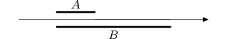
(a) $A$ and $B$ themselves.

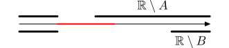
(b) $\mathbb{R}\setminus A$ and $\mathbb{R}\setminus B$.

Figure 2: The situation of Example 2. The red line highlights the Hausdorff distance between $A$ and $B$ (left), as well as their complements (right).

That $\left\|\mathrm{sd}_{A}-\mathrm{sd}_{B}\right\|_{\infty}$ is strictly stronger than $d_{H}(A,B)$ also manifests itself in the induced topology on the space of compact subsets of $\mathbb{R}^{n}$:

Example 3.

Let $A=[-1,1]$. For $k\in\mathbb{N}$, we define

$$A_{k}=A\setminus\left(-\frac{1}{k},\frac{1}{k}\right).$$

This defines a compact set $A_{k}\subset A$ for each $k$. Furthermore, $d_{H}(A,A_{k})=1/k\to 0$ as $k\to\infty$. In other words, $A_{k}\to A$ in the Hausdorff distance. However, $\mathrm{sd}_{A}(0)=-1$ while $\mathrm{sd}_{A_{k}}(0)=1/k$. In particular, $\mathrm{sd}_{A_{k}}\not\to\mathrm{sd}_{A}$.

Example 3 implies also that the reverse of (7),

$$\left\|\mathrm{sd}_{A}-\mathrm{sd}_{B}\right\|_{\infty}\leq C\cdot d_{H}(A,B),$$

can not hold for any constant $C$. Thus, one really needs both the ordinary and the complementary Hausdorff distance to get an upper bound on $\left\|\mathrm{sd}_{A}-\mathrm{sd}_{B}\right\|_{\infty}$. In other words, $d_{H}(A,B)$ and $\left\|\mathrm{sd}_{A}-\mathrm{sd}_{B}\right\|_{\infty}$ are not equivalent metrics. Compare also Example 2 in [2]: There, it is shown that the topologies induced by the ordinary and the complementary Hausdorff distance are not the same. This is done with a construction similar to Example 3.

2.3 The Maximum Distance Function

In the final part of this section, we would like to introduce another lower bound for $d_{H}(A,B)$. This additional bound may improve the approximation of $d_{H}(A,B)$ if we are not able to maximise over all $x\in\mathbb{R}^{n}$ but only, for instance, grid points. However, we ultimately come to the conclusion that this bound is probably not very useful for a practical computation of $d_{H}(A,B)$. This will be discussed further at the end of the current subsection. Hence, we will not make use of the results here in the later Section 3. Since the concepts are, nevertheless, interesting at least from a theoretical point of view, we still give a brief presentation here. As far as we are aware, these results have not been discussed in the literature before.

Our initial motivation is the following: We have seen in Theorem 1 that the Hausdorff distance $d_{H}(A,B)$ can be expressed as $\left\|d_{A}-d_{B}\right\|_{\infty}$. On the other hand, $\left\|\mathrm{sd}_{A}-\mathrm{sd}_{B}\right\|_{\infty}$ gives not the Hausdorff distance. If we are given $\mathrm{sd}_{A}$ and $\mathrm{sd}_{B}$ for the computation, this is unfortunate. While it is, of course, trivial to get $d_{A}$ and $d_{B}$ from the signed distance functions, this process throws away valuable information. In particular, the information from the signed distance functions at points inside the sets can not be used. By defining yet another type of “distance function”, which now gives the maximal distance to any point in a set, we get rid of this qualitative difference between interior and exterior points:

Definition 3.

Let $\Omega\subset\mathbb{R}^{n}$ be bounded. The maximum distance function of $\Omega$ is then

$$\mathrm{md}_{\Omega}(x)=\sup_{y\in\Omega}\left|x-y\right|.$$ (8)

Since $\Omega$ is bounded, this is well-defined for any $x\in\mathbb{R}^{n}$. If $\Omega$ is compact in addition, an analogous result to Lemma 1 holds.

Indeed, $\mathrm{md}_{\Omega}$ is always non-negative (assuming $\Omega\neq\emptyset$). For $\mathrm{md}_{\Omega}(x)$, it does not immediately matter whether $x\in\Omega$ or not. Furthermore, also the maximum distance function gives a lower bound on the Hausdorff distance, similar to (3):

Theorem 3.

Let $A,B\subset\mathbb{R}^{n}$ be compact and choose $x\in\mathbb{R}^{n}$ arbitrarily. Then

$$\left|\mathrm{md}_{A}(x)-\mathrm{md}_{B}(x)\right|\leq d_{H}(A,B).$$

Proof.

The proof is similar to the proof of Theorem 1: Let $x\in\mathbb{R}^{n}$ be given. There exist $y\in B$ with $\mathrm{md}_{B}(x)=\left|x-y\right|$ and $z\in A$ with $d_{A}(y)=\left|y-z\right|$. Note that $d_{H}(A,B)\geq\left|y-z\right|$ and $\mathrm{md}_{A}(x)\geq\left|x-z\right|$. Thus

$$\mathrm{md}_{B}(x)-\mathrm{md}_{A}(x)\leq\left|x-y\right|-\left|x-z\right|\leq\left|y-z\right|\leq d_{H}(A,B).$$

This completes the proof if we apply the same argument also with the roles of $A$ and $B$ exchanged. ∎

Unfortunately, the analogue of (4) does not hold. In fact, it is possible that $\mathrm{md}_{A}=\mathrm{md}_{B}$ everywhere on $\mathbb{R}^{n}$ but the sets $A$ and $B$ are quite dissimilar. Such a situation is depicted in Figure 3. Due to the “outer ring”, which is part of $A\cap B$, the maximum in (8) is always achieved with some $y$ from this ring. A typical situation is shown with the point $x$ and the red line, which highlights its maximum distance to both $A$ and $B$. Consequently, $\mathrm{md}_{A}=\mathrm{md}_{B}$ and the differences between $A$ and $B$ inside the ring are not “seen” by the maximum distance functions at all. Thus, we have to accept that $\left\|\mathrm{md}_{A}-\mathrm{md}_{B}\right\|_{\infty}<d_{H}(A,B)$ can be the case.

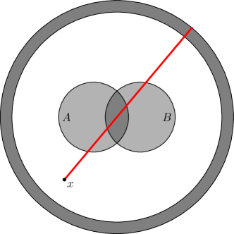
Figure 3: In the shown situation, $\mathrm{md}_{A}=\mathrm{md}_{B}$ while $A$ and $B$ are clearly not the same sets. Dark regions are $A\cap B$, while lighter regions are $A$ or $B$ alone. The red line highlights the maximum distance $\mathrm{md}_{A}(x)=\mathrm{md}_{B}(x)$ for some generic point $x$.

The situations where the maximum distance functions actually carry valuable information (as opposed to Figure 3) are actually similar to those characterised in Definition 5. For such situations, the additional information in $\mathrm{md}_{A}$ and $\mathrm{md}_{B}$ could, indeed, be used to improve the approximation of $d_{H}(A,B)$. However, as we will see below in Theorem 5, those are also the situations where (4) alone already gives a very close estimate of $d_{H}(A,B)$. In these cases, we are not really in need of additional information. On the other hand, for situations like Figure 3 also the approximation of $d_{H}(A,B)$ from grid points is actually difficult and extra data would be very desirable. But particularly for those situations, the maximum distance functions do not provide any extra data! Furthermore, it is not clear how $\mathrm{md}_{A}$ and $\mathrm{md}_{B}$ can actually be computed from, say, the level-set functions of $A$ and $B$. It seems plausible that those functions are the viscosity solutions of an equation similar to the Eikonal equation, and so it may be possible to develop either a Fast Marching scheme or some other numerical method. However, since we have just argued that we do not expect a real benefit from the usage of the maximum distance functions in practice, the effort involved seems not worthwhile. For the remainder of this paper, we will thus concentrate on Theorem 1 as the sole basis for our numerical computation of $d_{H}(A,B)$.

3 Estimation of the Error on a Grid

With the basic theoretical background of Section 2, let us now consider the situation on a grid. In particular, we assume that we have a rectangular, bounded grid in $\mathbb{R}^{n}$ with uniform spacing $h$ in each dimension. (While it is possible to generalise some of the results to non-uniform grids in a straight-forward way, we assume a uniform spacing for simplicity.) We denote the finite set of all grid points by $N$, and the set of all grid cells by $C$. For each cell $c\in C$, $N(c)$ is the set of all grid points that span the cell (i. e., its corners). For example, for a $k\times k$ grid in $\mathbb{R}^{2}$ that extends from the origin into the first quadrant, we have

$$\begin{split}N&=\left\{x_{ij}\;|\;i,j=0,\ldots,k-1,\;x_{ij}=(i,j)h\right\},\\ C&=\left\{c_{ij}\;|\;i,j=1,\ldots,k-1\right\},\;\;N(c_{ij})=\left\{x_{i-1,j-1},\,x_{i,j-1},\,x_{ij},\,x_{i-1,j}\right\}.\end{split}$$

Let us assume that we know the distance functions of $A$ and $B$ on each grid point, i. e., $d_{A}(x)$ and $d_{B}(x)$ for all $x\in N$. We furthermore assume that these values are known without approximation error. This is, of course, not realistic in practice. However, the approximation error in describing the geometries and computing their distance functions is a matter outside the scope of this paper. Finally, let us also assume that the grid is large enough to cover the sets. In particular: For each $y\in A\cup B$, there should exist a grid cell $c\in C$ such that $y$ is contained in the convex hull $\mathrm{co}\left(N(c)\right)$ of the corners of $c$. If this is not the case, the grid is simply inadequate to capture the geometrical situation.

3.1 Worst-Case Estimates

In order to approximate $d_{H}(A,B)$ from the distance functions on our grid, we make use of (4). In particular, we propose the following straight-forward approximation:

$$d_{H}(A,B)\approx\tilde{d}(A,B)=\max_{x\in N}\left|d_{A}(x)-d_{B}(x)\right|$$ (9)

From (3), we know that this is, at least, an exact lower bound. However, in the general case, an approximation error

$$0\leq\delta=\left|d_{H}(A,B)-\tilde{d}(A,B)\right|=d_{H}(A,B)-\tilde{d}(A,B)$$

will be introduced by using (9). This is due to the fact that we only maximise over grid points. The real maximiser of the supremum in (4), on the other hand, may not be a grid point.

Let us now analyse the approximation error $\delta$. We have seen in the proof of Theorem 1 that

$$d_{H}(A,B)=\sup_{y\in A\cup B}\left|d_{A}(y)-d_{B}(y)\right|=\max_{c\in C}\sup_{y\in\mathrm{co}\left(N(c)\right)}\left|d_{A}(y)-d_{B}(y)\right|.$$

Note that this is still an exact representation, with no approximation error introduced so far. We have just split up the supremum over $A\cup B$ into grid cells, but we still take into account all points contained in a grid cell, not just its corners. This is achieved by using the convex hull $\mathrm{co}\left(N(c)\right)$ instead of the finite set $N(c)$ alone. On the other hand, the approximation (9) can be formulated as

$$\tilde{d}(A,B)=\max_{c\in C}\max_{x\in N(c)}\left|d_{A}(x)-d_{B}(x)\right|.$$

Comparing both equations, we see that the approximation error $\delta$ is introduced precisely by the step from $\mathrm{co}\left(N(c)\right)$ to $N(c)$. We can now formulate and prove a very general upper bound on $d_{H}(A,B)$:

Theorem 4.

Let $x\in N$ be a grid point and $y\in\mathbb{R}^{n}$ be arbitrary. We set

$$t(x,y)=\left\{\begin{array}[]{rl}\left|x-y\right|&x\in A,\\ 2\left|x-y\right|&x\not\in A.\\ \end{array}\right.$$

For a cell $c\in C$, we define furthermore

$$\overline{d}(c)=\sup_{y\in\mathrm{co}\left(N(c)\right)}\min_{x\in N(c)}\left(\left|d_{A}(x)-d_{B}(x)\right|+t(x,y)\right).$$ (10)

Then

$$d\left(A\to B\right)\leq\max_{c\in C^{\prime}(A)}\overline{d}(c).$$

Here, $C^{\prime}(A)=\left\{c\in C\;|\;\mathrm{co}\left(N(c)\right)\cap A\neq\emptyset\right\}$ is the set of all grid cells which contain some part of $A$.

Similarly, $d\left(B\to A\right)$ and thus $d_{H}(A,B)$ can be estimated.

Proof.

We will show that

$$\sup_{y\in A\cap\mathrm{co}\left(N(c)\right)}\left|d_{A}(y)-d_{B}(y)\right|\leq\overline{d}(c)$$

for each $c\in C$. The claim then follows from (5). So choose $c\in C$, $y\in A\cap\mathrm{co}\left(N(c)\right)$ and $x\in N(c)$. It remains to verify that

$$\left|d_{A}(y)-d_{B}(y)\right|=d_{B}(y)\leq\left|d_{A}(x)-d_{B}(x)\right|+t(x,y).$$

Assume first that $x\in A$. Since $d_{B}$ has Lipschitz constant one, we really get

$$\left|d_{A}(x)-d_{B}(x)\right|+t(x,y)=d_{B}(x)+\left|x-y\right|\geq d_{B}(y)$$

in this case. Assume now $x\not\in A$. Since $y\in A$ and thus $d_{A}(y)=0$, Lipschitz continuity of $d_{A}$ implies that $d_{A}(x)\leq\left|x-y\right|$. Using this auxiliary result, we get that also in this case

$$\left|d_{A}(x)-d_{B}(x)\right|+t(x,y)\geq d_{B}(x)-d_{A}(x)+2\left|x-y\right|\geq d_{B}(x)+\left|x-y\right|\geq d_{B}(y).$$

Hence, the claim is shown. ∎

Even though the formulation of Theorem 4 is complicated, the idea behind it is quite simple: Since the distance functions are Lipschitz continuous, also the function $\left|d_{A}-d_{B}\right|$, which we have to maximise over $\mathrm{co}\left(N(c)\right)$ for each grid cell, is Lipschitz continuous. This allows us to estimate the maximum in terms of the function’s values at the corners (which are known). We are even allowed to try all corners and use the smallest resulting upper bound. This is what happens in (10). Furthermore, the Lipschitz constant depends on whether or not the corner is in $A$. (If it is, $d_{A}$ vanishes, which reduces the Lipschitz constant to just that of $d_{B}$. Otherwise, we have to use two as the full Lipschitz constant of $\left|d_{A}-d_{B}\right|$.) This is the role that $t(x,y)$ plays. It gives the “distance” between $x$ and $y$ based on the applicable Lipschitz constant.

Coupled with the fact that $\tilde{d}(A,B)$ is a lower bound for the exact Hausdorff distance, the upper bound in Theorem 4 allows us now to estimate $\delta$. However, evaluating (10) is difficult and expensive in practice (although it can be done in theory). Hence, we will now draw some conclusions that simplify the upper bound. As a first result, let us consider the worst case where $x\not\in A$ for all corners $x\in N(c)$ of some cell:

Corollary 1.

Theorem 4 implies for the error estimate:

$$\delta\leq\sqrt{n}\cdot h$$

Proof.

Let $c\in C$ be some grid cell and $y\in\mathrm{co}\left(N(c)\right)$. Then there exists $x\in N(c)$ such that

$$t(x,y)\leq 2\left|x-y\right|\leq 2\cdot\frac{\sqrt{n}\cdot h}{2}=\sqrt{n}\cdot h.$$

This is simply due to the fact that the grid cell’s longest diagonal has length $\sqrt{n}\cdot h$. Consequently, in the worst case the nearest corner $x$ has half that distance to $y$. Hence also

$$\begin{split}\min_{x\in N(c)}\left(\left|d_{A}(x)-d_{B}(x)\right|+t(x,y)\right)&\leq\max_{x\in N(c)}\left|d_{A}(x)-d_{B}(x)\right|+\min_{x\in N(c)}t(x,y)\\ &\leq\max_{x\in N(c)}\left|d_{A}(x)-d_{B}(x)\right|+\sqrt{n}\cdot h.\end{split}$$

This estimate can be used for $\overline{d}(c)$ from (10). Consequently, Theorem 4 implies

$$d\left(A\to B\right)\leq\max_{c\in C}\max_{x\in N(c)}\left|d_{A}(x)-d_{B}(x)\right|+\sqrt{n}\cdot h=\tilde{d}(A,B)+\sqrt{n}\cdot h.$$

Since the same estimate also works for $d\left(B\to A\right)$, the claim follows. ∎

Taking a closer look, though, the worst-case situation considered above is quite strange. In principle, it can happen that there is some cell $c$ with $A\cap\mathrm{co}\left(N(c)\right)\neq\emptyset$ but for which all corners are not in $A$. Such a situation is depicted in Figure 4. However, in practice such a case is very unlikely to occur. In particular, assume that we describe the set $A$ by a level-set function $\phi$, and that $\phi(x)>0$ for all corners $x\in N(c)$ of some grid cell $c$. In that case, there is no way of knowing whether, in reality, there is some part of $A$ inside the cell or not. The grid is simply too coarse to “see” such geometric details. Consequently, it makes sense to assume the simplest possible situation, namely that $A\cap\mathrm{co}\left(N(c)\right)=\emptyset$ for all such cells $c$. Thus, we make the following additional assumption:

Definition 4.

Consider grid cells $c\in C$ such that $x\not\in A$ for all corners $x\in N(c)$. If $\mathrm{co}\left(N(c)\right)\cap A=\emptyset$ for all those $c$, the grid is said to be suitable for $A$.

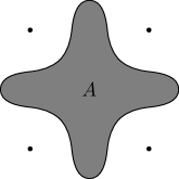
Figure 4: A possible pathological situation where the grid is not suitable for $A$.

In the case of a suitable grid (for both $A$ and $B$), we get the “reduced Lipschitz constant” in (10) for at least one corner per relevant cell. This allows us to lower the error estimate:

Corollary 2.

Let the grid be suitable for $A$ and $B$. Furthermore, we introduce the dimensional constant

$$\Delta_{n}=\sup_{y\in Q}\min\left(\left|y\right|,\,\min_{x\in N^{\prime}}2\left|x-y\right|\right).$$ (11)

Here, $Q=\left\{y\in\mathbb{R}^{n}\;|\;0\leq y_{i}\leq 1\text{ for all $i=1,\ldots,n$}\right\}$ is the unit square, and

$$N^{\prime}=\left\{x\in\mathbb{R}^{n}\;|\;x_{i}\in\left\{0,1\right\}\text{ for all $i=1,\ldots,n$}\right\}\setminus\left\{0\right\}$$

is the set of its corners except for the origin. Then,

$$\delta\leq\Delta_{n}\cdot h.$$

Proof.

Let $c\in C$ be a cell with $\mathrm{co}\left(N(c)\right)\cap A\neq\emptyset$. Since the grid is assumed to be suitable, we know that there exists at least one corner $x_{0}\in N(c)$ with $x_{0}\in A$. Hence, for arbitrary $y\in\mathrm{co}\left(N(c)\right)$,

$$\min_{x\in N(c)}t(x,y)\leq\min\left(\left|y-x_{0}\right|,\,\min_{x\in N(c)\setminus\left\{x_{0}\right\}}2\left|y-x\right|\right)\leq\Delta_{n}\cdot h.$$

With this, the claim follows as in the proof of Corollary 1. ∎

The most difficult part of Corollary 2 is probably the strange dimensional constant $\Delta_{n}$ defined in (11). This constant replaces the functions $t(x,\cdot)$ for $x\in N(c)$. It can be interpreted like this: Let spherical fronts propagate starting from all corners of the unit square $Q$. The front starting at the origin has speed one, while the other fronts have speed $1/2$. Over time, the fronts will hit each other, and will reach all parts of $Q$. The value of $\Delta_{n}$ is precisely the time it takes until all points in $Q$ have been hit by at least one front. For the case $n=2$, these arrival times are shown in Figure 5a. The correct value of $\Delta_{2}$ is the maximum attained at both spots with the darkest red (one in the north and one in the east). Figure 5b shows the maximising points (red and black) over the unit cube for $n=3$. Since the expression that is maximised in (11) is symmetric with respect to permutation of the coordinates, there are six maximisers. The highlighted one sits at the intersection of the spheres originating from the three corners marked in blue. Based on these observations and some purely geometrical arguments, one can calculate

$$\Delta_{1}=\frac{2}{3}\approx\numprint{0.67},\;\;\Delta_{2}=\frac{2}{3}\sqrt{5-\sqrt{7}}\approx\numprint{1.02},\;\;\Delta_{3}=\frac{2}{3}\sqrt{8-\sqrt{19}}\approx\numprint{1.27}.$$

These constants are a clear improvement over the estimate of Corollary 1. In fact, the bound in Corollary 2 is actually sharp. To demonstrate this, we will conclude this subsection with an example in two dimensions that really attains the maximal error $\delta=\Delta_{2}\cdot h$:

(a) Arrival times for $\Delta_{2}$.

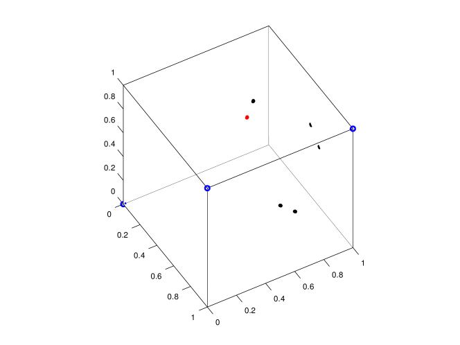
(b) Maximising points for $\Delta_{3}$.

Figure 5: The computation of $\Delta_{2}$ and $\Delta_{3}$ from the maximisation of the arrival times over $Q$.

Example 4.

For simplicity, assume $h=1$. We consider the situation sketched in Figure 6. Observe first that all grid points except $a$, $b$, $c$ and $d$ are part of $A\cap B$, and thus $d_{A}=d_{B}=0$ for them. Consequently, we only have to consider these four points in order to find $\tilde{d}(A,B)$. For symmetry reasons, it is actually enough to concentrate only on $a$ and $b$. The point $p$ corresponds to the position with maximal arrival time, as seen also in Figure 5a. It is characterised by requiring

$$\left|a-p\right|=\left|d-p\right|=\frac{r}{2},\;\;\left|b-p\right|=\left|c-p\right|=r.$$ (12)

Solving these equations for the coordinates of $p$ and the radius $r$ yields

$$p=\left(\frac{8-\sqrt{7}}{6},\;\frac{1}{2}\right),\;\;r=\frac{2}{3}\sqrt{5-\sqrt{7}}.$$

Note specifically that $r=\Delta_{2}$. (In fact, a construction similar to this one can be used to calculate $\Delta_{2}$ in the first place.) The relations (12) can also be seen in the sketch: The dotted circle has radius $r$ and centre $p$. The points $b$ and $c$ lie on it. The two smaller circles (which define the exclusion from $A$) have centres $a$ and $d$ with radius $r/2$, and $p$ lies on both of them.

$B$ is chosen in such a way that $p$ is also at the centre of its hole. Consequently, $p$ is the point in $A$ that achieves $d_{H}(A,B)=d\left(A\to B\right)=d_{B}(p)$. This is indicated by the red line. Let us also introduce $\rho$ as the width of the small ring between the dotted circle and the dark region. Then $\rho=d_{B}(b)$ and $d_{H}(A,B)=r+\rho$. Furthermore, note that

$$d_{A}(a)=\frac{r}{2},\;\;d_{B}(a)=\frac{r}{2}+\rho.$$

Hence,

$$\tilde{d}(A,B)=\left|d_{A}(a)-d_{B}(a)\right|=\left|d_{A}(b)-d_{B}(b)\right|=\rho.$$

This also implies that $\delta=r=\Delta_{2}\cdot h$, which is, indeed, the largest possible bound permitted by Corollary 2.

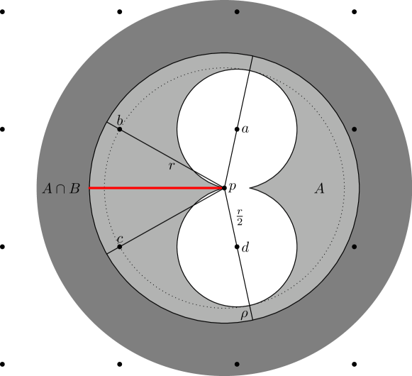
Figure 6: The situation considered in Example 4. The dark region is $A\cap B$, the lighter part inside the circle is $A\setminus B$. The red line indicates the Hausdorff distance $d_{H}(A,B)=d\left(A\to B\right)$.

3.2 External Hausdorff Distances

As we have promised, the situation from Example 4 shows that one can not, in general, expect a better error estimate than Corollary 2. However, considering Figure 6, we also observe that the situation there is quite strange. Thus, there is hope that we can get stronger estimates if we add some more assumptions on the geometrical situation. This is the goal of the current subsection. It will turn out in Theorem 5 that this is, indeed, possible. Consider, for example, Figure 7a: There, $d_{H}(A,B)=d\left(A\to B\right)=\left|x-y\right|$. Furthermore, all points $z$ along the external black line satisfy $\left|d_{A}(z)-d_{B}(z)\right|=\left|x-y\right|$. Consequently, all those points are maximisers of (4). If a grid point happens to lie somewhere on this line, $\tilde{d}(A,B)$ is exact. But even if this is not the case (as shown in the figure), $\left|d_{A}-d_{B}\right|$ will be very close to $\left|x-y\right|$ for grid points that are far away from the sets and close to the line. In all of these cases, we can expect $\tilde{d}(A,B)$ to be much closer to $d_{H}(A,B)$ than the bounds from the previous Subsection 3.1 tell us. Furthermore, the estimate will be more precise the further away we can go on the external line. Two conditions determine how far that really is: First, of course, the size of our finite grid is a clear restriction. Second, we need that $d_{A}(z)=\left|z-x\right|$ and $d_{B}(z)=\left|z-y\right|$ for the points $z$ on the external line that we consider. This means that $x$ and $y$ must be the closest points to $z$ of the sets $A$ and $B$, respectively. The latter is a purely geometrical condition on $A$ and $B$, and is not related to the grid. Let us formalise it:

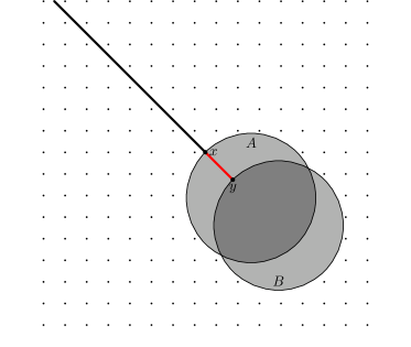
(a) The external line with $d_{H}(A,B)=\left|d_{A}-d_{B}\right|$.

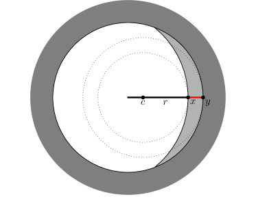
(b) External Hausdorff distance with a restricted $r$.

Figure 7: The situation of an external Hausdorff distance from Definition 5. The red lines indicate the Hausdorff distances $d_{H}(A,B)=d\left(A\to B\right)$. The dark regions are, as always, $A\cap B$, while the lighter parts are $A$ or $B$ alone.

Definition 5.

Assume that $d_{H}(A,B)=d\left(A\to B\right)=\left|x-y\right|>0$ with $x\in A$ and $y\in B$. Let $r>0$ and set $d=(x-y)/\left|x-y\right|$ as well as $c=x+rd$ and $R=r+d_{H}(A,B)$. We say that $A$ and $B$ admit an external Hausdorff distance with radius $r$ if

$$\overline{B_{r}\left(c\right)}\cap A=\left\{x\right\},\;\;\overline{B_{R}\left(c\right)}\cap B=\left\{y\right\}.$$ (13)

The condition in Definition 5 is quite technical, but it is relatively easy to understand and verify for concrete situations (as long as it is known where the Hausdorff distance is attained). It is related to the skeleton of the sets $A$ and $B$, for which we refer to Section 3.3 of [3]. We will see later in Corollary 3 that, for instance, convex sets admit an external Hausdorff distance for arbitrary radius $r$, and that Definition 5 applies in a lot of additional practical situations. Even for non-convex sets, an external Hausdorff distance with some restriction on the possible $r$ may be admissible. See, for instance, the situation in Figure 7b. A possible choice for $r$ and $c$ is shown there. (The furthest possible $c$ is at the end of the black line.) The dotted circles are $\overline{B_{r}\left(c\right)}$ and $\overline{B_{R}\left(c\right)}$. One can see that the inner one only touches $A$ at $x$, and the outer one does the same with $B$ at $y$. This is the geometrical meaning of (13). Due to this property, we know that $d_{A}(c)=\left|c-x\right|$ and $d_{B}(c)=\left|c-y\right|$. One can also verify that the condition (13) gets strictly stronger if we increase $r$. In other words, if an external Hausdorff distance with $r$ is admissible, this is automatically also the case for all radii $s<r$.

Based on this concept of external Hausdorff distances, we can now formalise the motivating argument about better error bounds for this situation:

Theorem 5.

Let $A$ and $B$ admit an external Hausdorff distance with $r>0$. Let $h$ be the grid spacing, and assume that the grid is chosen large enough. Then, for $h\to 0$,

$$\delta\leq\frac{n}{2}\frac{h^{2}}{r}+O\left(h^{3}\right).$$ (14)

Proof.

We use the same notation as in Definition 5. In particular, let $d_{H}(A,B)=d\left(A\to B\right)=\left|x-y\right|$ with $x\in A$ and $y\in B$. We also use $c$ and $R$ as in the definition. If $z$ is a point next to the straight line $x$–$c$, we can project it onto this line. Let the resulting point be called $c^{\prime}$, then $c$–$c^{\prime}$–$z$ and $x$–$c^{\prime}$–$z$ are right triangles. This situation is shown in Figure 8. According to the sketch, we set

$$\rho=R-\left|z-c\right|=R-\sqrt{a^{2}+b^{2}}.$$

Note that the dotted circle $B_{\rho}\left(z\right)$ is entirely contained in $B_{R}\left(c\right)$. By (13), this implies that $d_{B}(z)\geq\rho$. Since $x\in A$, we also know $d_{A}(z)\leq\left|z-x\right|=\sqrt{b^{2}+(r-a)^{2}}$. Both inequalities together yield

$$\tilde{d}(A,B)\geq\left|d_{A}(z)-d_{B}(z)\right|\geq d_{B}(z)-d_{A}(z)\geq R-\sqrt{a^{2}+b^{2}}-\sqrt{b^{2}+(r-a)^{2}}.$$

(Assuming that $z$ is a grid point.) On the other hand, since we have an external Hausdorff distance, also

$$d_{H}(A,B)=\left|d_{A}(c^{\prime})-d_{B}(c^{\prime})\right|=d_{B}(c^{\prime})-d_{A}(c^{\prime})=(R-a)-(r-a)$$

holds. Hence,

$$\delta=d_{H}(A,B)-\tilde{d}(A,B)\leq\sqrt{b^{2}+a^{2}}-a+\sqrt{b^{2}+(r-a)^{2}}-(r-a).$$ (15)

So far, $z$ was just an (almost) arbitrary grid point. We will now try to choose it in a way that reduces the bound on $\delta$ as much as possible. For this, observe that (15) contains two terms of the form $s\mapsto(\sqrt{b^{2}+s^{2}}-s)$ and that this function is decreasing in $s$. Thus, in order to get a small bound, we would like to choose both values of $s$, namely $a$ and $r-a$, as large as possible. Consequently, we want $a\approx r/2$. Let $m=(c+x)/2$ be the precise midpoint between $c$ and $x$. Since $\sqrt{n}\cdot h$ is the longest diagonal of the grid cells, there exists a grid point $z\in N$ with $\left|m-z\right|\leq\sqrt{n}/2\cdot h$. Choosing $c^{\prime}$ as the projection of $z$ onto the line $x$–$c$ as before, this implies that

$$a\geq\frac{r}{2}-\left|m-c^{\prime}\right|\geq\frac{r-\sqrt{n}\cdot h}{2},\;\;r-a\geq\frac{r-\sqrt{n}\cdot h}{2},\;\;b=\left|z-c^{\prime}\right|\leq\frac{\sqrt{n}}{2}h.$$

(Since $\left|m-z\right|^{2}=\left|m-c^{\prime}\right|^{2}+\left|z-c^{\prime}\right|^{2}$, not all of these estimates can be sharp at the same time. It may be possible to refine them and get smaller bounds below, but we do not attempt to do that for simplicity.) Substituting in (15) yields

$$\delta\leq\sqrt{nh^{2}+(r-\sqrt{n}\cdot h)^{2}}-(r-\sqrt{n}\cdot h).$$

Series expansion of this result for $h\to 0$ finally implies the claimed estimate (14).

Figure 8: Deriving the bound (15) in the proof of Theorem 5.

∎

A particular situation in which Definition 5 is satisfied is that of convex sets (see Figure 7a). For them, (14) holds with arbitrary $r$ as long as the grid is large enough to accommodate for the far-away points:

Corollary 3.

Let $A$ and $B$ be compact and convex. Then $A$ and $B$ admit an external Hausdorff distance for arbitrary $r>0$. Consequently, (14) applies for all $r$ for which the grid is large enough.

Proof.

We exclude the trivial case $A=B$, since (14) is obviously fulfilled for that situation anyway. Assume, without loss of generality, that $d_{H}(A,B)=d\left(A\to B\right)$. Let $x\in A$ and $y\in B$ be given with $d\left(A\to B\right)=\left|x-y\right|>0$ according to Lemma 1. Choose $r>0$ arbitrarily and let $c$ be as in Definition 5.

The assumption $d\left(A\to B\right)=d_{B}(x)=\left|x-y\right|$ means that $y$ is the closest point in $B$ to $x$. In other words, $B_{s}\left(x\right)\cap B=\emptyset$, where we have set $s=\left|x-y\right|$ for simplicity. This is depicted with the dotted circle (which is outside of $B$) in Figure 9. The dotted lines indicate half-planes perpendicular to the line $x$–$y$ and through $x$ and $y$, respectively. Assume for a moment that we have some point $z\in B$ that is “above” the “lower” half-plane. Due to convexity of $B$, this would imply that the whole line $z$–$y$ must be inside of $B$. This, however, contradicts $B_{s}\left(x\right)\cap B=\emptyset$ as indicated by the red part of $z$–$y$. Hence, the half-plane through $y$ separates $B$ and $x$. Similarly, we can show that the half-plane through $x$ separates $A$ and $c$: Assume that $z^{\prime}\in A$ is “above” this half-plane. Then $d_{B}(z^{\prime})>s$ must be the case, as shown by the blue line. But this is a contradiction, since $d_{B}(z^{\prime})\leq d\left(A\to B\right)=s$ for all $z^{\prime}\in A$. These separation properties of the half-planes, however, in turn imply (13). Thus, everything is shown.

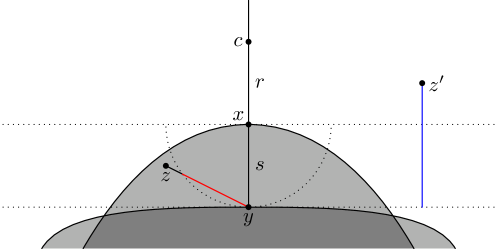
Figure 9: Sketch for the proof of Corollary 3.

∎

Let us also remark that the proof of Corollary 3 stays valid as long as the sets $A$ and $B$ are “locally convex” in a neighbourhood of $x$ and $y$. This is an important situation for a lot of potential applications: We already mentioned above that our own motivation for computing the Hausdorff distance is to measure convergence during shape optimisation. In this case, it is often the case that the Hausdorff distance is already quite small in relation to the sets. For a lot of these situations, the largest difference between the sets is attained in a way similar to Figure 9, even if the sets themselves need not necessarily be convex.

3.3 Numerical Demonstration

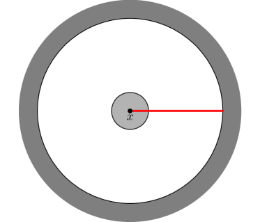
(a) Inner circle at the origin.

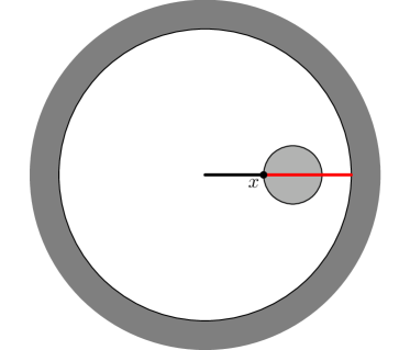
(b) Displaced inner circle.

Figure 10: The example situation (schematically) used for Subsection 3.3. We have a dark “outer ring” $A\cap B$ and a smaller circle $A\setminus B$ that is inside. The Hausdorff distance $d_{H}(A,B)=d\left(A\to B\right)$ is indicated with the red line. In right plot, the external line with $\left|d_{A}-d_{B}\right|=d_{H}(A,B)$ is also indicated.

To conclude this section, let us give a numerical demonstration of the results presented so far. The situation that we consider is depicted schematically in Figure 10: We have an “outer ring” which is part of both $A$ and $B$, and an inner circle (corresponding to $A\setminus B$) is placed within. Note that this is already a situation where we have non-convex sets. For the inner circle at the origin as in Figure 10a, no external Hausdorff distance is admissible. This is due to the fact that the point $x\in A$ that achieves $d_{H}(A,B)=d\left(A\to B\right)=d_{B}(x)$ is in the interior of $A$. If we displace the inner circle, the point $x$ will be on the boundary as soon as the origin is no longer part of $A$. In these situations, we have an external Hausdorff distance with a restricted maximal radius $r$. This is indicated in Figure 10b. In our calculations, the outer circle has a radius of nine and the inner circle’s radius is one. Figure 10 shows other proportions since this makes the figure clearer. However, qualitatively, the situations shown are exactly those that will be used in the following.

Let us first fix the grid spacing $h$ and consider the effect of moving the inner circle. The approximation error $\delta$ of the exact Hausdorff distance is shown (in units of $h$) in Figure 11. The blue curve shows $\delta$ under the assumption that $\mathrm{sd}_{A}$ and $\mathrm{sd}_{B}$ are known on the grid points without any approximation error. This is the situation we have discussed theoretically above. The red curve shows the error if we also compute the signed distance functions themselves using the Fast Marching code in [10]. This is a situation that is more typical in practice, where often only some level-set functions are known for $A$ and $B$. They are, most of the time, not already signed distance functions. Note that the grid was chosen such that the origin (and thus the optimal $x$ for small displacements) is at the centre of a grid cell and can not be resolved exactly by the grid. This yields the “plateau” in the error for small displacements. However, as soon as external Hausdorff distances are admitted, the observed error falls rapidly in accordance to Theorem 5. The “steps” in the blue and red lines are caused by the discrete nature of the grid. The black curve shows the expected upper bound, which is given by $\Delta_{2}$ for small displacements and by (14) for larger ones. (For our example situation, the maximum allowed radius $r$ in Definition 5 can be computed exactly.) One can clearly see that the theoretical and numerical results match very well in their qualitative behaviour.

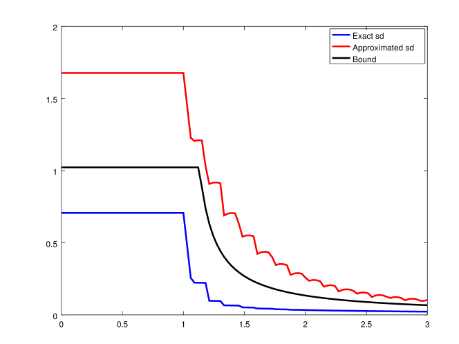
Figure 11: Error $\delta$ (relative to $h$) for a situation similar to Figure 10. The blue curve is based on exact signed distance functions. For the red curve, $\mathrm{sd}_{A}$ and $\mathrm{sd}_{B}$ were approximated as well. Black shows a combination of the error estimates from Corollary 2 (small displacement) and (14) (where applicable for larger displacements). The $x$-axis shows how far the inner circle is moved away from the origin.

Figure 12 shows how the error depends on the grid spacing $h$. The blue and red data is as before. In the upper Figure 12a, the inner circle is at the origin. This is the situation of Figure 10a, and corresponds to the very left of the curves in Figure 11. Here, the upper bound of Corollary 2 applies and is shown with the black curve. The convergence rate corresponds to $O\left(h\right)$, which can be seen clearly in the plot. On the other hand, the lower Figure 12b shows how $\delta$ behaves if we have an external Hausdorff distance. It corresponds to the very right in Figure 11, with the inner circle displaced from the origin similarly to Figure 10b. Here, Theorem 5 implies $O\left(h^{2}\right)$ convergence. Also this is, indeed, confirmed nicely by the numerical calculations. (While both plots look similar, note the difference in the scaling of the $y$-axes!)

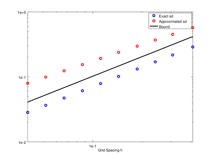
(a) Inner circle at the centre, as in Figure 10a.

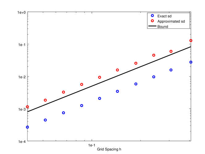
(b) Displaced inner circle, like Figure 10b.

Figure 12: Dependence of the error $\delta$ on the grid spacing $h$. The three data series are as in Figure 11.

4 Improvements by Randomising the Grid

Let us now take a closer look at the concept of external Hausdorff distances and, in particular, the error estimate in the proof of Theorem 5. An important ingredient for the resulting estimate (and the actual error) is how close grid points come to lie to the external line. We can emphasise this even more by reformulating the error estimate in the following way:

Lemma 2.

Let $A$ and $B$ admit an external Hausdorff distance with $r>0$. Choose $x\in A$, $y\in B$ and $d=(x-y)/\left|x-y\right|$ as in Definition 5. We denote by $\beta>0$ the minimum distance any grid point has to the part $L$ of the external line between $x+3/8\cdot rd$ and $x+5/8\cdot rd$, i. e.,

$$L=\left\{x+\tau\cdot rd\;|\;\tau\in\left[\frac{3}{8},\frac{5}{8}\right]\right\},\;\;\beta=\min_{z\in N}d_{L}(z)=\min_{z\in N}\min_{y\in L}\left|y-z\right|.$$ (16)

If the grid is large enough, then the error estimate

$$\delta\leq\frac{3}{r}\cdot\beta^{2}$$

holds for all grid spacings $h$ that are small enough.

Proof.

We base the proof on (15). Using the notation of Figure 8, let us consider points $c^{\prime}$ on the middle third $M$ of the external line. For them, $\min(a,\,r-a)\geq r/3$. Consequently, (15) implies

$$\delta\leq\sqrt{b^{2}+a^{2}}-a+\sqrt{b^{2}+(r-a)^{2}}-(r-a)\leq 2\cdot\left(\sqrt{b^{2}+\frac{r^{2}}{9}}-\frac{r}{3}\right)\leq\frac{3}{r}\cdot b^{2}.$$

The last estimate can be seen with a series expansion. This holds for $b$ being any distance (in normal direction) of a grid point $z$ to $M$. Furthermore, note that the interval $[3/8,\,5/8]$ is a strict subset of $[1/3,\,2/3]$, which implies that also $L$ is a strict subset of $M$. As long as $h$ is small enough, this means that we can find a suitable grid point such that $b\leq\beta$ holds. This finishes the proof. ∎

Of course, the distance $\beta$ between grid points and the line segment $L$ can always be estimated trivially by $\sqrt{n}/2\cdot h$. We did this in the proof of Theorem 5, and this leads precisely to the upper bound given in (14). The only difference to Lemma 2 is the smaller constant in (14). This is due to the very generous estimation we used in Lemma 2 for simplicity. We can now make an important observation: This is the absolutely worst-case estimate, which matches a situation as shown in Figure 7a. If the external line is not running “parallel” to the grid, we can expect that some of the grid points lie much closer to it (see Figure 13). Such a situation occurs, in particular, almost surely if the grid is placed “randomly” with respect to the geometry. This usually happens, for instance, if the original input data for a computation stems from real-world measurements in one way or another.

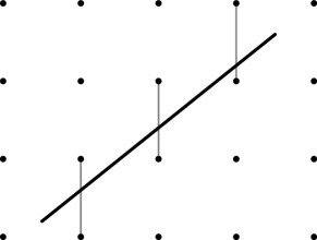
Figure 13: Random placement of a line segment in a grid and the corresponding estimation of the distance $\beta$ to the closed grid point.

In this section, we analyse the effect that such a random grid placement has on the resulting error bounds. We will see that we can show even stronger convergence than in Theorem 5 in this case. These estimates are based on Lemma 2. The crucial additional ingredient is a suitable upper bound for the minimum distance $\beta$. The idea we employ for that is illustrated in Figure 13: We look for edges of the grid that are intersected by the line segment $L$, and use the distance along such an edge to the next grid point as an upper bound for $\beta$. The finer the grid, the more such intersection edges appear. Each one of them gives us an additional “chance” to find a particularly short distance, and thus improve $\beta$. Consequently, it is interesting to know how many such edges are there for a particular line segment:

Lemma 3.

Let $L\subset\mathbb{R}^{n}$ be an arbitrary line segment with length $\lambda$, placed in a grid as shown in Figure 13. Then $L$ intersects at least $\left\lfloor\lambda/(\sqrt{n}\cdot h)\right\rfloor$ edges (or faces in 3D, cells in 4D and so on) of the grid, where $h>0$ is the grid spacing as usual. In particular, the line $L$ of (16) intersects at least $r/(5\sqrt{n})\cdot 1/h$ edges if $h$ is small enough.

Proof.

Since $\sqrt{n}\cdot h$ is the longest diagonal of a grid cell, every line segment of at least this length must intersect some edge. Our line $L$ of length $\lambda$ is made up of $\left\lfloor\lambda/(\sqrt{n}\cdot h)\right\rfloor$ such pieces, which shows the claim. The additional statement follows by noting that $\lambda=r/4$ for $L$ in (16) and that the estimate

$$\left\lfloor\frac{r}{4\sqrt{n}}\cdot\frac{1}{h}\right\rfloor\geq\frac{r}{5\sqrt{n}}\cdot\frac{1}{h}$$

is true if $h$ is sufficiently small. ∎

To further motivate this idea, let us continue Subsection 3.3 with more numerical examples. We use the same basic situation (that is shown schematically in Figure 10b), but add two randomised changes: First, the grid is randomly shifted in $x$- and $y$-direction up to a grid cell. This prevents any bias due to the placement of the coordinate system relative to the outer circle. Second, the inner circle is displaced in a random direction, which has the same effect as a random rotation of the grid. The resulting errors $\delta$ between the exact and approximated Hausdorff distances are plotted in Figure 14. These figures show the results of 1,000 runs with different randomisations. The bound of Theorem 5 is shown again with the black line, and it clearly holds true for all runs. Another observation, however, is that the error really decreases much faster on average: The red dots indicate the geometric mean over all runs; while not rigorously justified, this gives a rough first indication of the average convergence behaviour. A more representative analysis can be based on Figure 15: There, we show histograms of the approximated convergence orders for each of the individual runs. One can clearly see that most of the runs have, indeed, a stronger order than $O\left(h^{2}\right)$. For 2D, the median order is almost $O\left(h^{4}\right)$. For 3D, it is “only” about $O\left(h^{3}\right)$, but that is still a drastic improvement over Theorem 5. Also note that a tiny fraction of runs shows an order worse than $O\left(h^{2}\right)$. This is, however, not in contradiction to our theory and rather a numerical artefact: For them, the error is (due to good luck) already very small for coarse grids, so that the corresponding decrease seems slower for the grid sizes we considered. The error bound of (14) is, nevertheless, still true.

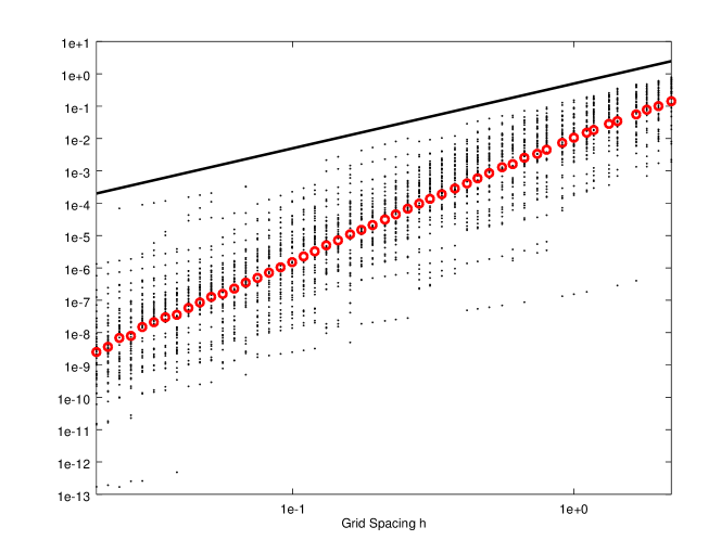
(a) 2D

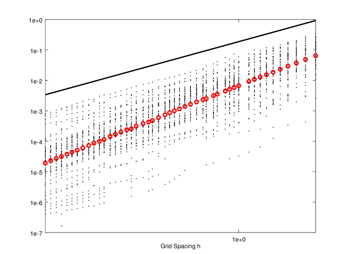
(b) 3D

Figure 14: The errors $\delta$ between the exact and approximated Hausdorff distances for the situation of Figure 10b with randomisation applied. The black line shows the bound of Theorem 5, the dots correspond to the results of individual runs. Their geometric mean is shown with red circles.

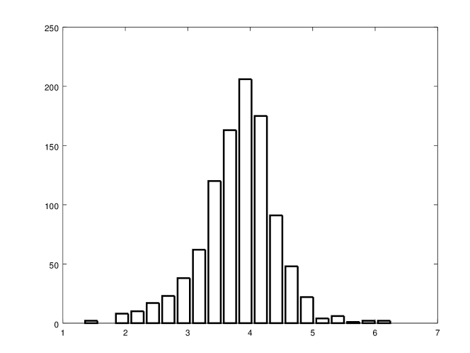
(a) 2D

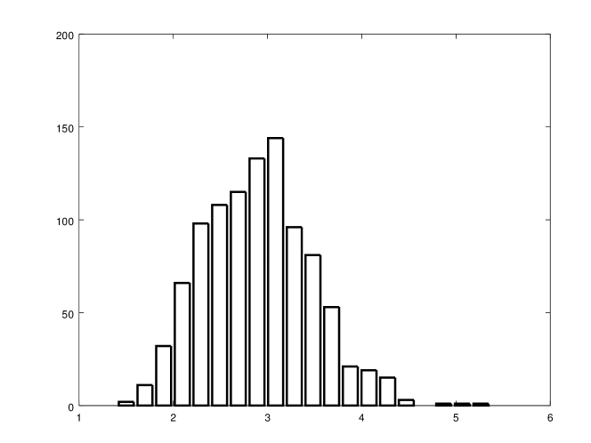
(b) 3D

Figure 15: Histogram of the approximated convergence orders for the runs in Figure 14.

4.1 Super-Quadratic Convergence in 2D

Let us now consider the randomised situation more thoroughly. In this subsection, we concentrate on the 2D case and will be able to show improved error bounds that hold almost surely if a randomisation is applied. These results will be complemented by a heuristic argument given in Subsection 4.2 that yields even better convergence rates for the “average case” and works in arbitrary dimension.

The main thing to do now is to find a bound on $\beta$ of (16). For this, consider Figure 13 again and assume $h=1$ for the moment. The distance between the line segment $L$ and the grid point below it along each intersected edge behaves then like $\left\lfloor x_{0}+ik\right\rfloor$, where $x_{0},k\in\mathbb{R}$ depend on the particular line in question and $i\in\mathbb{N}$ numbers the intersected grid edges. The analysis of such a sequence of numbers lies at the heart of the error bound shown later in this subsection:

Lemma 4.

Let $x_{0}\in\mathbb{R}$ and $k\in\mathbb{R}\setminus\mathbb{Q}$ be given. For $i\in\mathbb{N}$, we define $x_{i}=\left\lfloor x_{0}+ik\right\rfloor\in[0,1)$. Then, for arbitrary $N\in\mathbb{N}$, there are $i_{0},j_{0}\in\left\{0,\ldots,N\right\}$ such that $0<\epsilon=\left|x_{i_{0}}-x_{j_{0}}\right|\leq 1/N$. Furthermore, there is $m\in\left\{0,\ldots,K\right\}$ with $\left|x_{m}\right|\leq\epsilon$, where the maximum number $K$ of iterates necessary for achieving this condition satisfies

$$K\leq N\left\lceil\frac{1}{\epsilon}\right\rceil\leq\frac{2}{\epsilon^{2}}.$$

Proof.

Assume for a moment that $\left|x_{i}-x_{j}\right|>1/N$ for all $i,j=0,\ldots,N$ with $i\neq j$. This also implies that all intervals $I_{i}=[x_{i}-1/N,\,x_{i}+1/N]$ are disjoint. Since $\left|I_{i}\cap(0,1)\right|\geq 1/N$ and there are $N+1$ of the intervals, this is not possible. Thus, there exist $i_{0},j_{0}\in\left\{0,\ldots,N\right\}$ with $i_{0}\neq j_{0}$ and $\epsilon=\left|x_{i_{0}}-x_{j_{0}}\right|\leq 1/N$. It remains to show that $\epsilon>0$. Assume to the contrary that $\left|x_{i_{0}}-x_{j_{0}}\right|=0$. This means $\left|i_{0}-j_{0}\right|k\in\mathbb{N}$. But since $i_{0}\neq j_{0}$, this contradicts the assumption that $k\not\in\mathbb{Q}$. Thus, the first statement is shown.

Without loss of generality, let us now assume that $i_{0}<j_{0}$ and that $x_{i_{0}}<x_{j_{0}}$. Setting $p=j_{0}-i_{0}\in\mathbb{N}$, note that $p\in\left\{1,\ldots,N\right\}$ and $\left\lfloor pk\right\rfloor=\left|x_{i_{0}}-x_{j_{0}}\right|=\epsilon$. In other words, advancing $p$ iterates in the sequence increases the value of $x_{i}$ by $\epsilon$. With a similar argument to before, this implies that we cover the whole interval $[0,1]$ in at most $p\left\lceil 1/\epsilon\right\rceil$ iterations. This implies that $\left|x_{m}\right|\leq\epsilon$ for some $m\in\left\{0,\ldots,K\right\}$ with

$$K\leq p\left\lceil\frac{1}{\epsilon}\right\rceil\leq N\left\lceil\frac{1}{\epsilon}\right\rceil\leq\frac{1}{\epsilon}\left(\frac{1}{\epsilon}+1\right)\leq\frac{2}{\epsilon^{2}}.$$

∎

There are a few things to remark about the proof of Lemma 4: Note that we do not directly get an upper bound for the number of iterates required to get close to zero within a certain threshold. Instead, the sequence itself yields a distance $\epsilon$, and the number of iterates required is then defined in terms of $\epsilon$. If $\epsilon$ happens to be much smaller than $1/N$, we also need a lot more iterates. On the other hand, however, this larger number of iterates also brings us much closer to zero than $1/N$. There is a balance between closeness to zero and the number of iterates we need, but we have no direct control over either quantity. This also shows why it is crucial that $k$ is an irrational number: If it is not, it may happen that $\epsilon=0$. In this case, we are not guaranteed to ever come close to zero in a finite number of iterations since the sequence becomes periodic. In terms of our error analysis, this corresponds to the situation that the external line is parallel to the grid as depicted, for instance, in Figure 7a. Fortunately for us, however, the rational numbers have measure zero. This means that a randomly rotated grid will almost surely yield an irrational $k$ so that our analysis applies.

Another interesting observation is the following: The important first part of the proof establishes an estimate on the number of steps necessary before a pair of iterates occurs that are close to each other. On the first thought, this may sound as if the birthday paradox is applicable in this situation. This would improve the number of iterates necessary to $O\left(\sqrt{N}\right)$. Unfortunately for us, however, this is not true: In our case, the actual question is when $\left\lfloor pk\right\rfloor$ comes close to zero. It is only formulated in terms of a pair of iterates because this seems like the more natural formulation for the proof.

Finally, let us briefly discuss what happens if we try to use the same approach for the Hausdorff distance in $\mathbb{R}^{3}$: In this case, we consider a sequence of points on the unit square $[0,1)^{2}$. With the same argument as in the proof of Lemma 4, we can still show that a pair of iterates is within $1/N$ of each other if we perform $O\left(N^{2}\right)$ steps. (Note that the estimate gets drastically worse here!) It is not so clear, however, whether the second part of the proof can be adapted: On the one-dimensional interval $[0,1)$, repeatedly adding $\epsilon$ to an arbitrary point will eventually wrap around and yield an iterate close to zero. On the square in 2D, however, there is much more freedom for the sequence to iterate without ever getting close to the origin.

With the technical result of Lemma 4 in place, we can now use it to derive an estimate for $\beta$. Combining this with Lemma 2, we obtain an improved error estimate $\delta$ for the approximate Hausdorff distance:

Corollary 4.

Let $n=2$ and $A,B\subset\mathbb{R}^{2}$ admit an external Hausdorff distance with $r>0$. Assume that the grid is rotated randomly with respect to the external line. Then, with probability one, there exists a sequence $\left(h_{m}\right)_{m\in\mathbb{N}}\to 0$ of grid spacings tending to zero such that

$$\delta\leq\frac{45}{r^{2}}\cdot h_{m}h^{2}$$ (17)

for all $m\in\mathbb{N}$ and grids with $h<h_{m}$. In particular, the approximation error $\delta$ vanishes super-quadratically in the grid spacing.

Proof.

For $m\in\mathbb{N}$, choose $\epsilon_{m}\in(0,\,1/m]$ according to Lemma 4 and define

$$h_{m}=\frac{\epsilon^{2}r}{10\sqrt{n}}\;\;\Leftrightarrow\;\;\epsilon_{m}=\sqrt{\frac{10\sqrt{n}}{r}}\cdot\sqrt{h_{m}}.$$

Then clearly $h_{m}\to 0$ as $m\to\infty$. Furthermore, this definition ensures that the line segment $L$ of (16) intersects at least $2/\epsilon_{m}^{2}$ edges of any grid with $h\leq h_{m}$ according to Lemma 3.

As discussed above, the intersections of the line segment $L$ with grid edges (see Figure 13) can be described by a sequence like $\left\lfloor x_{0}+ik\right\rfloor$ after scaling the grid cells to size one. Note that a random rotation of the grid ensures $k\in\mathbb{R}\setminus\mathbb{Q}$ with probability one. Thus, Lemma 4 is applicable and yields that $\beta\leq\epsilon_{m}h$, where the additional factor $h$ can be added since our grid has cells of size $h\times h$ instead of unit size. Thus, Lemma 2 yields

$$\delta\leq\frac{3}{r}\cdot\epsilon_{m}^{2}h^{2}=\frac{30\sqrt{2}}{r^{2}}\cdot h_{m}h^{2}\leq\frac{45}{r^{2}}\cdot h_{m}h^{2}.$$

∎

Let us emphasise again that Corollary 4 only shows super-quadratic convergence and $O\left(h^{3}\right)$ along a particular sequence of grids, not cubic convergence in general. Since Lemma 4 does not give us any control over $\epsilon$, we also do not have any knowledge about the resulting sequence $\left(h_{m}\right)_{m\in\mathbb{N}}$ along which third-order convergence occurs. In practice, however, the bound in (17) seems to be quite conservative and usually an overestimation of the error. This matches also the behaviour seen in Figure 15a, which suggests that most of the runs show an empirical convergence order stronger than $O\left(h^{3}\right)$.

4.2 A Heuristic, Statistically-Motivated Estimate

While Corollary 4 gives a rigorously proven estimate, it is not clear how to extend the result to situations in more than two dimensions. Furthermore, the result is rather a conservative worst-case estimate than a practical bound on the expected average error. In this subsection, we give a different argument leading to stronger estimates that match the empirical results of Figure 15 more closely. This argument works in arbitrary space dimension, although the statement gets weaker the higher the dimension is. Also note that the main idea is only heuristically motivated and cannot be recovered in a formal proof. Consequently, all of this subsection will be written in an informal way without rigorously proving any statements.

We still base our estimate on Lemma 2, but replace Lemma 4 by the following heuristic idea: If the line segment $L$ intersects a large enough number of grid edges and is not parallel to the grid in any way, it seems plausible to assume that the intersection distances $\left\lfloor x_{0}+ik\right\rfloor$ follow roughly a uniform distribution on $[0,1)$. In a rigorous setting, this is of course not true—we do not consider independent random numbers at all, but correlated iterates of a deterministic sequence. Empirically, however, this assumption seems to be justified relatively well: The sequence can be compared to the well-known linear congruential generators for pseudo-random numbers (see, for instance, Section 3.1 of [13]). They are among the simplest and statistically weakest PRNGs, but their weaknesses seem to be irrelevant for our situation. See also Figure 16: This plot shows a histogram of 10,000 iterates of such a sequence. One can clearly see that while the distribution seems not to be perfectly uniform, it is quite close. The more iterates we use, the more uniform the distribution gets. Since we are interested in the limit of fine grids, i. e., $h\to 0$, this corresponds to a large number of intersected edges. Thus, it seems reasonable to assume that the intersections between the line segment $L$ and grid edges follow such a uniform distribution.

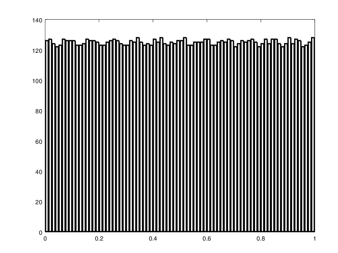
Figure 16: Histogram of 10,000 iterates in a sequence $\left\lfloor x_{0}+ik\right\rfloor$ with randomly chosen $x_{0},k\in[0,1]$.

This idea can be applied also in three and more dimensions: Instead of intersections along grid edges, we consider intersections of $L$ with faces of the grid cells in 3D. For them, we may (with the same heuristic justification) assume that they follow a uniform distribution on the square $[0,1)^{2}$. In even higher dimensions, this approach can be generalised further. Thus, let us assume that $X_{1},\ldots,X_{N}$ is a sequence of independent random variables that follow a uniform distribution on $[0,1)^{n-1}$. To replace Lemma 4 and find an estimate on $\beta$ for Lemma 2, we have to analyse the statistical properties of their minimum distance to the origin, i. e., of the derived random variable

$$X=\min(\left|X_{1}\right|,\,\ldots,\,\left|X_{N}\right|).$$

For simplicity, we will not analyse $X$ directly. Instead, we base our computations on random variables $Y_{i}$ that are uniformly distributed on the set

$$Q_{n}=\left\{x\in[0,\infty)^{n-1}\;|\;\left|x\right|<\sqrt{n-1}\right\}\subset\mathbb{R}^{n-1}.$$ (18)

This is a superset of $[0,1)^{n-1}$ and a spherical sector. For 3D, the set $Q_{3}$ is illustrated in Figure 17. Since the additional regions of $Q_{n}$ with respect to $[0,1)^{n-1}$ are far away from the origin, the corresponding minimum $Y$ is “larger than” $X$ with respect to important properties such as the expectation value or quantiles. Furthermore, with an appropriate scaling, one can also produce a subset of $[0,1)^{n-1}$ from $Q_{n}$. This implies that $X$ and $Y$ differ, roughly speaking, at most by a dimensional constant. Thus, we can use $Y$ for our analysis of the resulting convergence order.

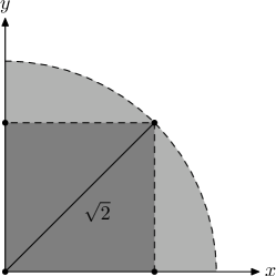
Figure 17: Relation between the quarter circle $Q_{3}$ of (18) and the square $[0,1)^{2}$. The latter is filled dark grey, with the additional regions of $Q_{3}$ light grey.

Next, we compute the density function for a random variable $\left|Y_{i}\right|$. For this, we are interested in the question what distance a uniformly placed point on $Q_{n}$ has from the origin. For $n\in\mathbb{N}$, let us denote the volume of the $n$-dimensional unit ball $B_{1}\left(0\right)\subset\mathbb{R}^{n}$ by $\omega_{n}$. For a general derivation of these constants, see Theorem 26.13 in [17]. Furthermore, note that the surface measure of a spherical shell with radius one is given by $n\omega_{n}$ according to Observation 26.24 in [17]. It is then straight-forward to express the density function $f(r)$ for a particular distance $r=\left|Y_{i}\right|$ with these constants as

$$f(r)=\frac{r^{n-2}\cdot(n-1)\omega_{n-1}}{\left(\sqrt{n-1}\right)^{n-1}\cdot\omega_{n-1}}=(n-1)^{\frac{3-n}{2}}\cdot r^{n-2}.$$

Note that it is trivial to check that this density function is normalised, i. e.,

$$\int_{0}^{\sqrt{n-1}}f(r)\,dr=(n-1)^{\frac{3-n}{2}}\int_{0}^{\sqrt{n-1}}r^{n-2}\,dr=1.$$

Building on $\left|Y_{i}\right|$, it remains to find the distribution of the minimum $Y$ of $N$ such random variables. In the case $Y=\left|Y_{1}\right|$, we know that $Y$ takes the norm of $Y_{1}$ and that all other points $Y_{2},\ldots,Y_{N}$ must have a norm at least as large. The probability density for this to happen is consequently

$$\tilde{g}(r)=f(r)\left(\int_{r}^{\sqrt{n-1}}f(\rho)\,d\rho\right)^{N-1}=(n-1)^{N\frac{3-n}{2}}\cdot r^{n-2}\cdot\left((n-1)^{\frac{n-3}{2}}-\frac{r^{n-1}}{n-1}\right)^{N-1}.$$

Since any of the $N$ variables could be the minimum, the density function of $Y$ is given by

$$g(r)=N\cdot\tilde{g}(r)=N\cdot f(r)\left(\int_{r}^{\sqrt{n-1}}f(\rho)\,d\rho\right)^{N-1}.$$

Again, one can show that $g$ is normalised by integrating over $r\in[0,\sqrt{n-1})$.

Let us now compute the expectation value $\mathbb{E}\left(Y\right)$. This quantity tells us how close the minimum distance of a grid point is on average to the line segment $L$. Again, the computation is straight-forward but technical. One finds

$$\mathbb{E}\left(Y\right)=\int_{0}^{\sqrt{n-1}}r\cdot g(r)\,dr=N\sqrt{n-1}\cdot\mathrm{B}\left(\frac{n}{n-1},\,N\right)=N\sqrt{n-1}\cdot\Gamma\left(\frac{n}{n-1}\right)\cdot\frac{\Gamma\left(N\right)}{\Gamma\left(N+\frac{n}{n-1}\right)},$$

where $\mathrm{B}\left(\cdot,\,\cdot\right)$ and $\Gamma\left(\cdot\right)$ are the beta and gamma functions, respectively. See Chapter 5 of [4] for more details about these special functions. We are particularly interested in the limit of fine grids, corresponding to $N\to\infty$. The asymptotic behaviour in this limit can be derived from 5.11.12 in [4], yielding

$$\mathbb{E}\left(Y\right)\sim N\cdot\frac{\Gamma\left(N\right)}{\Gamma\left(N+\frac{n}{n-1}\right)}\sim N\cdot N^{-\frac{n}{n-1}}\sim N^{-\frac{1}{n-1}}.$$ (19)

For $n=2$, one can also compute the percentiles of $Y$ exactly. They show precisely the same asymptotic behaviour.

Finally, let us discuss what (19) implies for the convergence order of $\delta$. For this, note first that $N\sim 1/h$ according to Lemma 3. The minimum distance $\beta$ of (16) is given by $hX$ after scaling the grid cells to unit size (matching the definition of $X$). As discussed above, we approximate this value by

$$\beta\approx h\cdot\mathbb{E}\left(Y\right)\sim h\cdot h^{\frac{1}{n-1}}.$$

Thus, Lemma 2 implies that we can expect the approximation error to behave like

$$\delta\sim\beta^{2}\sim h^{2}\cdot h^{\frac{2}{n-1}}=h^{\frac{2n}{n-1}}.$$

In other words, we get, indeed, a stronger average convergence order than $O\left(h^{2}\right)$ of Theorem 5. The additional factor shrinks with increasing space dimension. For $n=2$, we get $O\left(h^{4}\right)$. With $n=3$, the expected order is $h^{3}$. Note that this matches precisely the empirical results found in Figure 15.

5 Conclusion and Outlook

In this paper, we have discussed the relation between the Hausdorff distance $d_{H}(A,B)$ of two sets and their (signed) distance functions. This allowed us to state a method for computing $d_{H}(A,B)$ based on these distance functions $d_{A}$ and $d_{B}$. They can be easily computed, for instance, if the sets themselves are described in a level-set framework. Furthermore, we were able to analyse the approximation error made if the distance functions are only known on a finite grid (which is mostly the case in applications). To the best of our knowledge, such an error analysis has not been carried out before. We were able to derive a general and sharp estimate in Corollary 2. For the more regular situation characterised in Definition 5, our result of Theorem 5 implies an even lower error bound: In this case, the error is at most $O\left(h^{2}\right)$, where $h$ is the grid spacing. With a random rotation of the grid, even better convergence rates can be achieved. We have rigorously shown super-quadratic convergence for geometries in $\mathbb{R}^{2}$ in this case, and given a heuristic derivation of the average convergence order. All of our results are confirmed by numerical experiments. Nevertheless, there remain a lot of areas open for further investigations. In particular, we believe that the following open questions would be interesting targets of further research:

• We have not given a general formula for the constants $\Delta_{n}$ in arbitrary space dimensions. While cases with $n>3$ are, arguably, not so important, it could still be interesting to consider a general dimension $n$. It is probably not too hard to devise a method of assembling the system of equations that characterises $\Delta_{n}$ similarly to (12).

• Going even further, is it possible to find an efficient algorithm to evaluate (10) in a general situation? If this was possible, one could exploit Theorem 4 directly instead of resorting to approximations like Corollary 2. This is particularly interesting, since it would allow to couple information about $\left|d_{A}(x)-d_{B}(x)\right|$ on the corners $x$ of a grid cell with the corresponding Lipschitz constants in $t(x,\cdot)$. Doing this on a per-cell basis could improve the error bounds even further for an actual computation.

• Our definition of external Hausdorff distances in Definition 5 is straight-forward to verify for concrete situations and we argued why we believe that a lot of practical shapes fall into this category. It would, nevertheless, be interesting to further analyse the class of geometries that admit such an external Hausdorff distance.

• While we believe that our discussion of the effect of randomisation in Section 4 forms a sound basis both theoretically and for practical applications, the stochastic error analysis started there opens up a lot of possibilities for further refinement.

References

- [1] Mikhail J. Atallah. A Linear Time Algorithm for the Hausdorff Distance Between Convex Polygons. Computer Science Technical Reports, Paper 363, 1983. http://docs.lib.purdue.edu/cstech/363/.
- [2] D. Chenais and Enrique Zuazua. Finite-Element Approximation of 2D Elliptic Optimal Design. Journal de Mathématiques Pures at Appliquées, 85(2):225–249, 2006.
- [3] Michel C. Delfour and Jean-Paul Zolésio. Shapes and Geometries: Metrics, Analysis, Differential Calculus, and Optimization. Advances in Design and Control. SIAM, second edition, 2011.
- [4] NIST Digital Library of Mathematical Functions. http://dlmf.nist.gov/, Release 1.0.9 of 2014-08-29. Online companion to [12].
- [5] John W. Eaton, David Bateman, Søren Hauberg, and Rik Wehbring. GNU Octave version 4.0.0 manual: a high-level interactive language for numerical computations, 2015. https://www.gnu.org/software/octave/doc/interpreter/.
- [6] Daniel P. Huttenlocher, Gregory A. Klanderman, and William J. Rucklidge. Comparing Images Using the Hausdorff Distance. IEEE Transactions on Pattern Analysis and Machine Intelligence, 15(5):850–863, September 1993.
- [7] Oliver Jesorsky, Klaus J. Kirchberg, and Robert W. Frischholz. Robust Face Detection Using the Hausdorff Distance. In Proceedings of the Third International Conference on Audio- and Video-based Biometric Person Authentication, Lecture Notes in Computer Science, pages 90–95. Springer, 2001.
- [8] Moritz Keuthen and Daniel Kraft. Shape Optimization of a Breakwater. Inverse Problems in Science and Engineering, 24(6):936–956, 2016. http://dx.doi.org/10.1080/17415977.2015.1077522.
- [9] Daniel Kraft. A Hopf-Lax Formula for the Level-Set Equation and Applications to PDE-Constrained Shape Optimisation. In Proceedings of the 19th International Conference on Methods and Models in Automation and Robotics, pages 498–503. IEEE Xplore, 2014.
- [10] Daniel Kraft. The level-set Package for GNU Octave. Octave Forge, 2014–2015. http://octave.sourceforge.net/level-set/.
- [11] Sarana Nutanong, Edwin H. Jacox, and Hanan Samet. An Incremental Hausdorff Distance Calculation Algorithm. In Proceedings of the VLDB Endowment, volume 4, pages 506–517, 2011.
- [12] F. W. J. Olver, D. W. Lozier, R. F. Boisvert, and C. W. Clark, editors. NIST Handbook of Mathematical Functions. Cambridge University Press, New York, NY, 2010. Print companion to [4].
- [13] Sheldon M. Ross. Simulation. Academic Press, fifth edition, 2013.
- [14] Oliver Schütze, Xavier Esquivel, Adriana Lara, and Carlos A. Coello Coello. Using the Averaged Hausdorff Distance as a Performance Measure in Evolutionary Multiobjective Optimization. IEEE Transactions on Evolutionary Computation, 16(4):504–522, 2012.
- [15] James A. Sethian. A Fast Marching Level Set Method for Monotonically Advancing Fronts. Proceedings of the National Academy of Sciences, 93(4):1591–1595, 1996.
- [16] Dong-Gyu Sim, Oh-Kyu Kwon, and Rae-Hong Park. Object Matching Algorithms Using Robust Hausdorff Distance Measures. IEEE Transactions on Image Processing, 8(3):425–429, March 1999.
- [17] James Yeh. Real Analysis: Theory of Measure and Integration. World Scientific, second edition, 2006.