Isochrone fitting of Galactic globular clusters – I. NGC 5904

Abstract

We present new isochrone fits to colour-magnitude diagrams of the Galactic globular cluster NGC 5904 (M5). We utilise 29 photometric bands from the ultraviolet to mid-infrared by use of the data from the Hubble Space Telescope, Gaia DR2, Wide-field Infrared Survey Explorer, Sloan Digital Sky Survey (SDSS), and other photometric data. In our isochrone fitting we use the PAdova and TRieste Stellar Evolution Code, the MESA Isochrones and Stellar Tracks, the Dartmouth Stellar Evolution Program, and a Bag of Stellar Tracks and Isochrones both for the solar-scaled and enhanced He and $\alpha$ abundances with a metallicity about [Fe/H]$=-1.33$ adopted from the literature. All tools provide us with estimates of the distance, age, and extinction law to the cluster. The best-fit distance, true distance modulus, and age are $7.4\pm 0.3$ kpc, $14.34\pm 0.09$ mag, and $12.15\pm 1.00$ Gyr, respectively. The derived distance agrees with the literature, including the Gaia DR2 parallax with its known global zero-point correction. All the data and models, except some UV and SDSS data, agree with the extinction law of Cardelli-Clayton-Mathis with $R_{\mathrm{V}}=3.60\pm 0.05$ and $A_{\mathrm{V}}=0.20\pm 0.02$ mag. This extinction is twice as high as generally accepted due to a rather high extinction between 625 and 2000 nm. An offset of the model colours instead of the high extinction in this range is a less likely, yet possible explanation of the discovered large deviations of the isochrones from the data.

1 Introduction

Galactic globular clusters (GCs) have been considered as an ideal laboratory to verify and calibrate the stellar evolution theory and to study the evolution of the Galaxy in general. Despite the fact that during the last two decades some evidence for multiple populations in most GCs became available (Gratton et al., 2004), many GCs have a dominant stellar population which is convenient for isochrone modelling and deriving some information about the cluster.

Theoretical stellar evolution models allow one to determine the age, distance, metallicity, and reddening to the cluster. Modern observations have given rise to an abundance of new results regarding the reliable isochrone fitting simultaneously in all possible ultraviolet (UV), optical and infrared (IR) bands for all stages of the stellar evolution, such as the main sequence (MS), its turn-off (TO), the subgiant branch (SGB), red giant branch (RGB), horizontal branch (HB), and asymptotic giant branch (AGB). On the one hand, new accurate photometry of individual stars in many GCs has been provided recently by the Hubble Space Telescope (HST) from the Wide Field and Planetary Camera 2 (WFPC2) (Layden et al., 2005), Wide Field Camera 3 (WFC3) UV Legacy Survey of Galactic Globular Clusters (Piotto et al., 2015; Soto et al., 2017) and Advanced Camera for Surveys (ACS) survey of Galactic globular clusters (Sarajedini et al., 2007), the Wide-field Infrared Survey Explorer (WISE) (Wright et al., 2010), the Gaia DR2 (Gaia Collaboration et al., 2018a), the Sloan Digital Sky Survey (SDSS) (York et al., 2000), the United Kingdom Infrared Telescope Infrared Deep Sky Survey (UKIDSS) (Hewett et al., 2006; Hambly et al., 2008; Hodgkin et al., 2009), the Panoramic Survey Telescope and Rapid Response System (Pan-STARRS) (Bernard et al., 2014), and other projects. On the other hand, modern theoretical models of the stellar evolution have been adopting to non-scaled-solar abundances, with enhanced helium and $\alpha$-elements which are typical for GCs.

As a result, new, more accurate isochrone fitting in many photometric bands has revealed new issues. For example, Barker & Paust (2018, hereafter BP18) have shown that ‘three stellar evolution models available with HST/WFC3 and HST/ACS bandpasses all produce good fits in visible and IR bands. However, all of them fail to match GC color-magnitude diagram (CMD) morphology in the UV.’ BP18 used extinction values for each of the filters, i.e. the wavelength-extintion dependance (or the extinction law, or the reddening curve) from Schlafly & Finkbeiner (2011). In this case, a precise theoretical model with a precise extinction law would provide the same dereddened distance modulus, metallicity, He abundance, $\alpha$-enhancement, and age, but different extinction for each band. However, the results of BP18 do not confirm this. BP18 attributed the discrepancies of their results to some imperfection of the models used. Yet, this may manifest that some real extinction laws to the GCs, which were considered by BP18, may differ from the law of Schlafly & Finkbeiner (2011). We note that the ‘standard’ extinction law of Cardelli, Clayton & Mathis (1989, hereafter CCM89) with the extinction-to-reddening ratio $A_{\mathrm{V}}/E(B-V)\equiv R_{\mathrm{V}}=3.1$, which is typically engaged in the calculation of isochrones, may also be far from reality in some cases.

Thus, isochrone fitting of a multi-band photometry based on some accurate estimates of metallicity, He abundance and $\alpha$-enhancement from spectroscopy and providing some convergent values of distance and age, as well as some extinction values for a set of wavelengths, seems to be a good method to verify the theoretical stellar evolution models and to find the best extinction laws in the lines of sights to GCs. For example, Hendricks et al. (2012) have used a combination of broadband near-infrared and optical Johnson-Cousins photometry to study the extinction law along the line of sight to the GC M4, assuming the validity of the CCM89 extinction law with $R_{\mathrm{V}}$ as a derived parameter. The five-band photometry, which they used in their study, provides enough information to derive $R_{\mathrm{V}}$. However, these data seem to be not enough to reveal a difference between a real extinction law to M4 and the one from CCM89. In this paper our ambition is to derive an extinction law to a GC as real as possible, using a much more extended set of photometric bands than before.

The aim of our study is to fit CMDs for the GC NGC 5904 (M5), for which a photometry in different bands (UV, optical, near-IR, and mid-IR) is available. With a fixed metallicity, He abundance, $\alpha$-enhancement, we are about to derive the most probable estimates of the age and distance to this GC and draw a realistic extinction law to it. Also, we will estimate the accuracy of the isochrones under consideration.

NGC 5904 is a GC at RA(2000)$=15^{h}18^{m}33^{s}$ and DEC(2000)$=+2\degr 04\arcmin 52\arcsec$ or $l=3.859\degr$ and $b=+46.796\degr$. The most comprehensive database of GCs by Harris (1996), revision of 2010, provides a distance to it of 7.5 kpc, reddening $E(B-V)=0.03$ mag, [Fe/H]$=-1.29$, and apparent visual distance modulus $(m-M)_{\mathrm{V}}=14.46$. Besides the wealth of available photometry, NGC 5904 is selected by us as a GC with no strong evidence for multiple CMD sequences, with accurate spectroscopic estimates of its metallicity, He abundance, and $\alpha$-enhancement, with low foreground and differential reddening, but with quite discrepant estimates of the foreground reddening from various data sources.

Rather different estimates of $E(B-V)$ for NGC 5904 include:

• $0.00\pm 0.02$ (Green et al., 2015),

• $0.02\pm 0.04$ (Arenou, Grenon & Gomez, 1992),

• $0.03\pm 0.02$ (Meisner & Finkbeiner, 2015),

• $0.03\pm 0.02$ (Schlafly & Finkbeiner, 2011),

• $0.04\pm 0.03$ (Drimmel, Cabrera-Lavers & López-Corredoira, 2003),

• $0.04\pm 0.03$ (Lallement et al., 2018),

• $0.04\pm 0.03$ (Schlegel, Finkbeiner & Davis, 1998, hereafter SFD),

• $0.07\pm 0.02$ (Green et al., 2018),

• $0.10\pm 0.04$ (Gontcharov, 2009, 2012b), and

• $0.12\pm 0.04$ (Gontcharov, 2017).

These estimates are not independent. For example, Meisner & Finkbeiner (2015), Schlafly & Finkbeiner (2011), Drimmel, Cabrera-Lavers & López-Corredoira (2003), and Lallement et al. (2018) have similar reddening zero points by use of the same data from SFD or by use of SFD as the prior for a poor dataset at such a high latitude ($b\approx 47\degr$). More details on this topic are presented by Gontcharov & Mosenkov (2017b, 2018, 2019).

These reddening estimates originate from observational results for very different wavelengths, which were inter- or extrapolated to $E(B-V)$ mostly by use of the CCM89 extinction law with $R_{\mathrm{V}}=3.1$. In the case of other extinction law for the dust medium between us and NGC 5904, this inter- or extrapolation may give such discrepant estimates of $E(B-V)$. For example, we calculate here the values $E(B-V)$ for Gontcharov (2012b) and Gontcharov (2017) from their original estimates $E(J-K_{s})=0.056\pm 0.02$ and $0.066\pm 0.02$ mag, respectively, assuming the extinction coefficient $E(J-K_{s})/E(B-V)=0.533$ for our stars (mostly with $5000<T_{\mathrm{eff}}<7000$ K) from Casagrande & VandenBerg (2014). However, an increase of this extinction coefficient with another extinction law would decrease the $E(B-V)$ estimates of Gontcharov (2012b) and Gontcharov (2017) and make them closer to the others.

Yet, a deviation of the extinction law is not the only possible reason of this diversity of the reddening estimates. In addition, we refer the reader to Gontcharov & Mosenkov (2018) who discuss some other reasons: some systematic errors of the estimates from SFD, Meisner & Finkbeiner (2015) and their followers, as well as a low accuracy of the estimates from Arenou, Grenon & Gomez (1992) due to a lack of high latitude stars in their sample.

Thus, these reddening data sources may be more or less reliable for describing the dust medium between us and NGC 5904. These data sources, except Schlafly & Finkbeiner (2011) and Green et al. (2018), have been verified by Gontcharov & Mosenkov (2017a, b, 2018) in their ability to put stars with the best Gaia DR1 Tycho–Gaia Astrometric Solution parallaxes (Michalik, Lindegren & Hobbs, 2015) among the isochrones in the Hertzsprung–Russell diagram. It has been found that the mean $E(B-V)$ at high Galactic latitudes behind the Galactic dust layer seems to be underestimated by Green et al. (2015), Meisner & Finkbeiner (2015), Drimmel, Cabrera-Lavers & López-Corredoira (2003) and SFD, while best estimated by Gontcharov (2012b) and Gontcharov (2017). For NGC 5904, we see the same lineup of the estimates. Therefore, the case of NGC 5904 seems to be suitable for further testing, whether lower or higher reddening estimates at such a high latitude are more reliable. Anyway, such a large diversity of the reddening estimates should be explained. It is important not only for exploring the nature of GCs, but also for improving the reddening/extinction estimates.

An attention to the large uncertainty (30 per cent at best) of these estimates should be paid. Up to now, this issue has not been considered thoroughly. For example, An et al. (2009, hereafter APM) in their tables 6, 8 and 10 provided systematic errors of an isochrone fitting for NGC 5904. They suggested a 20 per cent error in $E(B-V)$ from SFD. Consequently, they stated that the distance uncertainty dominates in the uncertainty of the resulting model colour, distance modulus, and age. However, the error of the emission-to-reddening calibration of SFD is 0.028 mag (SFD). Hence, this error appears to be 70 per cent instead of 20 per cent. With this estimate it is evident from tables 6, 8 and 10 of APM that the uncertainty of the reddening (and, consequently, of the extinction law) dominates.

The deviation of the extinction law is not the only explanation of the systematic colour offset of the isochrones from the observations in CMDs. It can also be explained by some errors associated with the detailed bandpass shape, absolute flux calibration, accepted colour-$T_{\mathrm{eff}}$ relation, and with other colour-dependent imperfections of the model isochrones, providing some inherent offsets of the model colours (see Clem et al. (2004); Kucinskas et al. (2006); Casagrande & VandenBerg (2014, 2018a); Choi et al. (2018); VandenBerg & Denissenkov (2018).

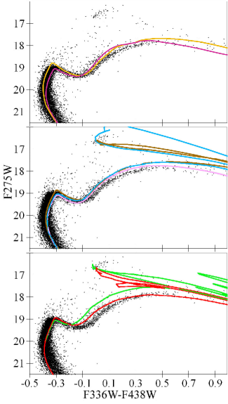
Figure 6: $F336W-F438W$ versus $F275W$ CMD of NGC 5904 with the best-fit parameters from Table 3 and the isochrones from DSEP solar-scaled (yellow) and DSEP He and $\alpha$ enhanced (magenta) – upper plot, old BaSTI solar-scaled (brown), old BaSTI He and $\alpha$ enhanced (light purple), and new BaSTI solar-scaled (blue) – middle plot, PARSEC solar-scaled (green) and MIST solar-scaled (red) – lower plot.

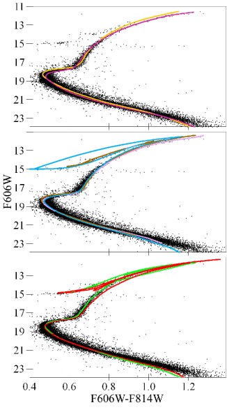
Figure 7: The same as Fig. 6 but for $F606W-F814W$ versus $F606W$.

However, these reasons would lead to some similar offsets for different GCs. Yet, figures 5–8 in APM for the isochrone fitting of the CMDs show quite different offsets for different GCs. Hence, these discrepancies are mostly due to an inaccurate representation of some properties of these GCs. Among such properties, the metallicity is well-estimated for these GCs, while some reasonable variations of age, He and $\alpha$ abundance could not shift the isochrones considerably. Therefore, only the extinction law, which they used in their study, seems to be responsible for the observed offsets.

Nevertheless, the systematic accuracy of the models and isochrones used should be estimated. Our approach may be fruitful in this way, since ‘the consistency of predicted colour-T_eff relations can be tested by determining if the same interpretation of the data (including discrepancies between theory and observations) is found on many different CMDs’ (Casagrande & VandenBerg, 2018a). Hereafter, we refer any systematic colour offset of an isochrone from observations as the corresponding reddening, though it can be partially or completely due to an imperfection of the isochrone.

This paper is organised as follows. We discuss the metallicity of NGC 5904 in Sect. 2. In Sect. 3 we describe the photometry used. In Sect. 4 we describe different theoretical models of the stellar evolution and consequent isochrones. We also draw some immediate conclusions from their application to the CMDs with the ‘canonical’ distance and reddening from Harris (1996). The results of our isochrone fitting are presented in Sect. 5 and discussed in Sect. 6. We summarise our main findings and conclusions in Sect. 7.

2 Metallicity

We adopt the spectroscopic estimate of metallicity [Fe/H]$=-1.33\pm 0.06$ derived for NGC 5904 by Carretta et al. (2009c) within an abundance scale well-defined from a large, precise and homogeneous data-set of [Fe/H] abundances of GCs. This estimate seems to obsolete the spectroscopic ones of Gratton, Quarta & Ortolani (1986) ($-1.42\pm 0.05$) and Carretta & Gratton (1997) ($-1.11\pm 0.11$). Another spectroscopic estimate [Fe/H]$=-1.36\pm 0.07$ (Kraft & Ivans, 2003), based on a different abundance scale, seems to obsolete the estimate $-1.17\pm 0.01$ by Sneden et al. (1992). Other spectroscopic estimates, such as $-1.40\pm 0.06$ (Zinn & West, 1984), even being on different abundance scales, tend to be within [Fe/H]$=-1.33\pm 0.10$. This uncertainty of $\pm 0.1$ dex corresponds to the uncertainty of colours of $<\pm 0.01$ mag at the TO, MS, SGB, HB, and fainter halves of the RGB and AGB, while up to $0.03$ mag at brighter halves of the RGB and AGB. The latter uncertainty is still lower than some uncertainties of the models dominating at the brighter halves of the RGB and AGB. It is seen in CMDs, for example, from Fig. 1–2 and 6–15 in the Appendix, where different models with the same [Fe/H]$\approx-1.33$ provide isochrones several hundredths magnitudes as bluer, as redder the fiducial sequence at the brighter halves of the RGB and AGB. This is a reason to pay more attention to the TO, SGB, MS than to the RGB and AGB in our isochrone fitting.

Carretta et al. (2009a) and Carretta et al. (2009b) found large star-to-star abundance variations for NGC 5904. For example, for the majority of investigated stars they found $-0.2<$[O/Fe]$<+0.4$. The average values are [O/Fe]$=+0.08\pm 0.23$, [Na/Fe]$=+0.25\pm 0.24$, [Mg/Fe]$=+0.41\pm 0.07$, [Al/Fe]$=+0.27\pm 0.29$, and [Si/Fe]$=+0.30\pm 0.05$. This suggests an enhanced average $\alpha$ abundance with its large variations from star to star. Moreover, Dell’Agli et al. (2018) have provided some evidence for an enhanced He abundance of $0.25<Y<0.31$ for the stars which they considered in NGC 5904. Hence, hereafter we consider both the scaled-solar and He-$\alpha$-enhanced isochrones for the same [Fe/H], age, reddening, and distance (except for the models with the scaled-solar abundances only) to bracket the observed scatter of the cluster abundances. We test the difference between the scaled-solar and He-$\alpha$-enhanced isochrones and, consequently, the importance of taking into account the He-$\alpha$-enhancement. In the case of a large difference, we fit the isochrones to the CMD so that the bulk of stars appear between the scaled-solar and non-scaled-solar isochrones of the same [Fe/H], age, and distance.

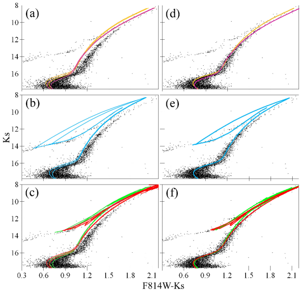
Figure 1: $F814W-K_{s}$ versus $K_{s}$ CMD of NGC 5904 with the isochrones from (a) and (d) DSEP solar-scaled (yellow), DSEP He and $\alpha$ enhanced (magenta), (b) and (e) new BaSTI solar-scaled (blue), (c) and (f) PARSEC solar-scaled (green) and MIST solar-scaled (red). The left column of the plots shows the pairs of the isochrones for 11 (left in the pair) and 13 Gyr (right in the pair) for the distance and reddening from Harris (1996) (7.5 kpc and $E(B-V)=0.03$ mag) and the CCM89 extinction law with $R_{V}=3.1$. The right column of the plots shows the best fit isochrones for the age, distance and reddening from Table 3.

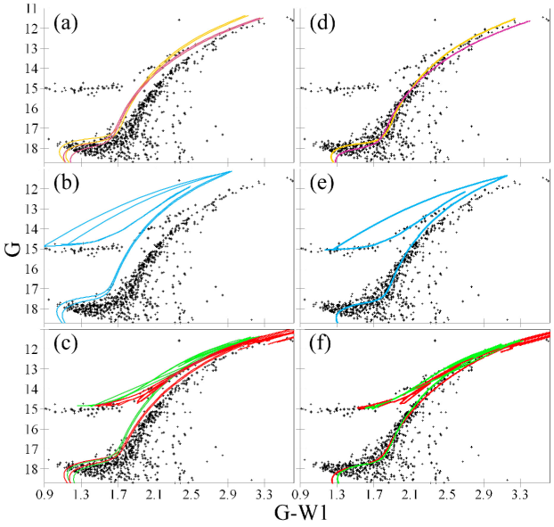
Figure 2: The same as Fig. 1 but for $G-W1$ versus $G$.

3 Photometry

To create CMDs for NGC 5904, we use the following photometry in 29 filters:

• 11472 stars with the photometry in the $F275W$, $F336W$ and $F438W$ filters from the HST WFC3 UV Legacy Survey of GCs (Piotto et al., 2015; Soto et al., 2017),

• 48860 stars with the photometry in the $F606W$ and $F814W$ filters from the HST ACS GC Survey (Sarajedini et al., 2007),

• 7582 stars with the HST WFPC2 photometry in the $F555W$ and $F814W$ filters (Layden et al., 2005),

• 6136 stars with the Gaia DR2 photometry in the $G$, $G_{\mathrm{BP}}$ and $G_{\mathrm{RP}}$ filters for the stars identified as NGC 5904 members by Gaia Collaboration et al. (2018c),

• 877 stars with the WISE photometry in the $W1$ band among the Gaia DR2 stars identified as NGC 5904 members by Gaia Collaboration et al. (2018c),

• 3493 stars with the UKIDSS LAS photometry in the $H$ filter among the Gaia DR2 stars identified as NGC 5904 members by Gaia Collaboration et al. (2018c),

• from 50925 to 58591 stars (depending on the filter) with the $UBVRI$ photometry (Viaux et al., 2013),

• 14379 stars with the $J$ and $K_{s}$ photometry obtained with SOFI at the New Technology Telescope (NTT) and with NICS at the National Telescope Galileo (TNG) (Coppola et al., 2011),

• from 9088 to 27803 stars (depending on the filter) with the SDSS photometry in the $ugriz$ filters (An et al., 2008, 2009).

• 17250 stars with both the Pan-STARRS and $UBVRI$ photometry, 2157 stars common to Pan-STARRS and Gaia, 1510 stars common to Pan-STARRS and WISE, as well as the fiducial sequences derived by Bernard et al. (2014) in the five bands of the Pan-STARRS1 photometric system ($g_{\mathrm{P1}}$, $r_{\mathrm{P1}}$, $i_{\mathrm{P1}}$, $z_{\mathrm{P1}}$, and $y_{\mathrm{P1}}$).

The effective wavelengths $\lambda_{\mathrm{eff}}$ in nm and the median precision of the photometry before eliminating stars with poor photometry are given for each filter in Table 1. Each star has a photometry in some, not necessarily in all filters.

Table 1: The effective wavelength (nm) and median precision of the photometry (mag) for the filters under consideration.

Telescope Filter $$\lambda_{\mathrm{eff}}$$ Median precision

HST/WFC3 274 0.02

HST/WFC3 329 0.02

Various 354 0.03

SDSS 360 0.08

Various 437 0.02

HST/WFC3 437 0.01

SDSS 471 0.04

Pan-STARRS1 480 0.01

Gaia DR2 514 0.04

HST/WFPC2 541 0.03

Various 547 0.01

HST/ACS 588 0.01

Pan-STARRS1 620 0.01

SDSS 621 0.04

Gaia DR2 625 0.01

Various 667 0.03

SDSS 743 0.05

Pan-STARRS1 746 0.01

Gaia DR2 762 0.03

HST/ACS 794 0.01

Various 812 0.01

HST/WFPC2 837 0.02

Pan-STARRS1 860 0.01

SDSS 885 0.10

Pan-STARRS1 960 0.01

NTT/TNG 1229 0.03

UKIDSS 1629 0.02

NTT/TNG 2147 0.04

WISE 3316 0.05

Based on the distribution of stars by the precision of their photometry, we select only stars with errors of less than 0.05 mag in the WFC3 and ACS colours, 0.055 mag in the WFPC2 colour, 0.05 mag in the $UBVRI$ colours, 0.06 mag in the Gaia and Gaia – UKIDSS colours, 0.10 mag in the Gaia – WISE colours, 0.05 mag in the $J-K_{s}$ colour, 0.06 mag in the SDSS colours, and 0.05 mag in Pan-STARRS colours.

Finally, we have 5 multicolour series in the optical range: HST (WFC3 and ACS), Gaia, $UBVRI$, SDSS, and Pan-STARRS. We have cross-identified them with each other and with the IR photometry, either with NTT/TNG $J$ and $K_{s}$, or UKIDSS $H$, or WISE $W1$. Only the HST WFPC2 photometry from Layden et al. (2005) is not cross-identified to the remaining data. It covers only the MS and partially the SGB, thus, providing a lower accuracy of the derived age and distance (they are, thus, taken fixed as 12 Gyr and 7.4 kpc, respectively), yet, a fairly high accuracy of the derived reddening. Therefore, the WFPC2 data are used for independent control only.

These photometric data allow us to consider and fit isochrones to more than 100 CMDs with different colours between the UV and middle IR. Each of the five multicolour series provides us with independent results. Additional results are derived for several IR colours.

4 Theoretical models and isochrones

To fit the CMDs of NGC 5904, we use the following theoretical models of the stellar evolution for creating isochrones:

• the PAdova and TRieste Stellar Evolution Code (PARSEC) (Bressan et al., 2012) with [Fe/H]$=-1.35$, $Z=0.00068$, $Y=0.25$, [$\alpha$/Fe]$=0$, mass loss 0.2 and the solar $Z=0.0152$,

• the MESA Isochrones and Stellar Tracks (MIST) (Paxton et al., 2011, 2013; Dotter, 2016; Choi et al., 2016) with [Fe/H]$=-1.35$, $Z=0.00066$, $Y=0.25$, [$\alpha$/Fe]$=0$, rotation $v_{\mathrm{initial}}/v_{\mathrm{critical}}=0.4$ and the solar $Z=0.0142$,

• the Dartmouth Stellar Evolution Program (DSEP) (Dotter et al., 2007, 2008), scaled-solar abundance with [Fe/H]$=-1.35$, $Z=0.00074$, $Y=0.246$, [$\alpha$/Fe]$=0$ and enhanced abundance with [Fe/H]$=-1.35$, $Z=0.0013$, $Y=0.33$, [$\alpha$/Fe]$=+0.40$, both with the solar $Z=0.0189$,

• A Bag of Stellar Tracks and Isochrones (BaSTI) in the two versions: the old version (Pietrinferni et al., 2004, 2006, 2013) , scaled-solar abundance with [Fe/H]$=-1.27$, $Z=0.0010$, $Y=0.246$, [$\alpha$/Fe]$=0$ and enhanced abundance with [Fe/H]$=-1.31$, $Z=0.0019$, $Y=0.30$, [$\alpha$/Fe]$=+0.5$, both with the solar $Z=0.019$; the new version (Hidalgo et al., 2018) with [Fe/H]$=-1.35$, $Z=0.000701$, $Y=0.2478$, [$\alpha$/Fe]$=0$, overshooting, diffusion, mass loss 0.3 and the initial solar $Z=0.0172$ and $Y=0.2695$.

• the isochrones from APM with [Fe/H]$=-1.5$, [$\alpha$/Fe]$=+0.3$ for the SDSS filters are used here only for testing because they draw the MS and TO only, and only for the ages 11.22 and 12.59 Gyr (both ages give the same accuracy of the fits).

Table 2: The fiducial sequence for NGC 5904 $F814W$ (HST ACS) versus $K_{s}$. The complete table is available online.

$$F814W$$

16.20 16.4

16.05 16.2

15.90 16.0

15.75 15.8

15.60 15.6

… …

Unfortunately, the current releases of PARSEC and MIST include the scaled-solar models only.

We note that the rotating and non-rotating MIST models give indistinguishable isochrones.

For every CMD we calculate the cluster fiducial sequence defined as the locus of the number density peaks on the CMD. This sequence represents a colour-magnitude relation for single stars of a dominant population in a cluster. We calculate the fiducial sequence as series of the median points in magnitude bins that have a size which varies as a function of the number of stars and photometric errors from 0.1 to 0.2 mag. This is an usual approach presented, for example, by Layden et al. (2005), An et al. (2008), Hendricks et al. (2012), Bernard et al. (2014), and VandenBerg & Denissenkov (2018). An example fiducial sequence for $F814W$ (HST ACS) versus $K_{s}$ is presented in Table 2. All other fiducial sequences can be provided on request.

We note that the fiducial sequences for NGC 5904 are relatively easily defined due to (i) a high degree of the completeness of the stellar samples under consideration, at least, between the HB and TO, (ii) low differential reddening, (iii) low contamination from foreground/background stars at such a high latitude, and (iv) low percentage of stars with a different age/metallicity.

The colour of the fiducial sequence for the faintest stars depends on their distance from the cluster’s center. This may be due to a contamination of the periphery of the cluster by the field stars or due to a crowding effect in the centre. However, this shift of the fiducial sequence is always $<0.01$ mag, i.e. negligible.

To derive the best reddening, distance, and age, we calculate the isochrones for a grid of some reasonable ages (10–14 Gyr with a step of 0.5 Gyr), distances (6.5–8.5 kpc with a step of 0.1 kpc) and reddenings [between $-0.1$ mag and the value calculated from $E(B-V)=0.12$ (the highest estimate in Sect. 1) and the CCM89 extinction law with $R_{\mathrm{V}}=5$, with a step of 0.005 mag]. Then we select the isochrone with a minimal total offset between the empirical fiducial points and their theoretical equivalents on this isochrone. To pay less attention to the RGB and AGB in our isochrone fitting, as discussed in Sect. 2, we consider only fiducial points at the TO, SGB, HB, the brighter part of the MS (limited by $<21$ mag for the optical bands) and the part of the RGB fainter than the HB, if the isochrone and the data cover these ridges.

The distance is better constrained by the magnitudes of the HB and SGB, the age – by the length and slope of the SGB and by the magnitude difference between the HB and SGB, while the reddening – by the overall colour offset of the isochrone w.r.t. the fiducial sequence.

Some changes in each parameter resulted in noticeably better or worse fits while the other parameters remained constant. These changes vary from colour to colour, but typically are 1 Gyr ($\approx$8 per cent) in age, 200 pc ($\approx$3 per cent) in distance, and 0.005 mag ($\approx$10 per cent) in reddening. We consider these values as preliminary estimates of the uncertainties of the fitting.

4.1 Immediate conclusions

Some immediate conclusions for a further fitting can be made from the fitting of the isochrones with the ‘canonical’ distance 7.5 kpc and reddening $E(B-V)=0.03$ mag from Harris (1996) together with the CCM89 extinction law with $R_{\mathrm{V}}=3.1$. The CMDs $F814W-K_{s}$ versus $K_{s}$ and $G-W1$ versus $G$ appear quite informative. They are presented in the left plots of Fig. 1 and 2, respectively, with the isochrones overimposed. Each isochrone is presented as a pair for the ages 11 (left) and 13 Gyr (right). This covers a range with the most probable estimates of the age for NGC 5904 from the literature. Yet, it is seen that the isochrones in each pair differ only on the TO, SGB and blue HB. This means that, on the one hand, the age is poorly defined by the fitting, while, on the other hand, any reasonable variations of the age could not eliminate the evident isochrone-fiducial offset.

An almost correct vertical position of the isochrones w.r.t. the HB and the SGB shows that the accepted distance of 7.5 kpc is quite close to the truth.

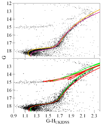
Figure 14: The same as Fig. 6 but for $G-H_{\mathrm{UKIDSS}}$ versus $G$.

Another important immediate conclusion from Fig. 1 and 2 is that DSEP shows quite little (few hundredths of mag) difference between the scaled-solar and He-$\alpha$-enhanced isochrones of the same [Fe/H], age, reddening, and distance. The same is evident from the next figures for all the colours, both for DSEP and old BaSTI. We explain this by the fact that with the same [Fe/H] the $\alpha$-enhancement makes the star cooler, whereas He-enhancement makes it hotter. Finally, they nearly compensate each other: an example is shown by Viaux et al. (2013, their figure 14, (b) and (d)). Thus, we can use the scaled-solar isochrones as an acceptable description for this GC.

The most important immediate conclusion from Fig. 1 and 2 is that the Harris’s $E(B-V)=0.03$ mag gives a noticeable colour offset of all the isochrones from the bulk of the stars. The same is typical for the other CMDs. Naturally, it can be solved by accepting a higher reddening. However, as mentioned in Sect. 1, this colour offset may be due to an offset of the model colours rather than due to the underestimated reddening. Anyway, any reasonable variation of metallicity, abundance, age, and distance cannot eliminate this offset.

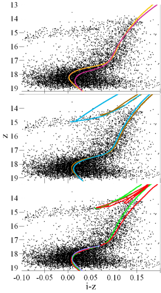
Figure 11: The same as Fig. 6 but for $i-z$ versus $z$. The additional isochrone from APM for the TO and SGB is shown together with the PARSEC and MIST ones as the violet curve.

Indeed, for any model and isochrone an increase of a parameter shifts the isochrone w.r.t. the fiducial sequence as follows [see also figure 11 of Choi et al. (2018)]:

• the increasing He abundance makes the RGB bluer, the SGB shorter, and the SGB less s-shaped;

• the increasing $\alpha$-enhancement makes the isochrone redder and fainter;

• the increasing age makes the SGB shorter and the HB-SGB magnitude difference larger;

• the increasing distance makes the isochrone fainter;

• the increasing reddening makes the isochrone redder and fainter;

• the increasing extinction law parameter, such as $R_{\mathrm{V}}$, makes any optical-IR isochrone redder and fainter.

Hence, for a fixed reddening there are only three ways to shift an isochrone redward: (i) a lower He abundance, or (ii) a higher $\alpha$ abundance, or (iii) a different extinction law, e.g. with a higher $R_{\mathrm{V}}$. Yet, both the abundances are tightly constrained by the spectroscopy. Moreover, the scaled-solar and He-$\alpha$-enhanced isochrones almost coincide. Thus, a higher reddening, or another extinction law, or a model colour improvement are the only solutions.

The right plots of Fig. 1 and 2 present the best fits with the derived age, distance and reddening (more generally, isochrone-fiducial colour offset) given in Table 3.

Table 3: The results of the isochrone fitting for various models and colours in comparison with the same reddenings predicted from Harris (1996). The values used to derive the average age and distance are highlighted with bold. The adopted values of age and distance are highlighted with italic.

PARSEC MIST DSEP Old BaSTI New BaSTI APM Harris

$$E(F275W-F336W)$$ 0.03

age, Gyr 11.5 13.0 11.0 11.5 11.5

distance, kpc 7.5 6.9 8.3 7.1 7.2

0.03

age, Gyr 12.0 12.5 11.0 12.0 12.5

distance, kpc 7.5 7.1 7.5 7.3 7.5

0.04

age, Gyr 11.5 13.5 12.0 12.5 13.0

distance, kpc 7.3 7.0 7.2 6.8 7.2

0.03

age, Gyr 12.0 13.5 12.5 12.5 12.5

distance, kpc 7.5 7.4 7.3 7.3 7.6

0.04

age, Gyr 12.0 12.0 12.0 12.0 12.0

distance, kpc 7.4 7.4 7.4 7.4 7.4

0.04

age, Gyr 11.5 12.5 11.5 12.5

distance, kpc 7.6 7.6 7.4 8.4

0.02

age, Gyr 11.5 12.5 12.0 11.0 12.5

distance, kpc 7.6 7.1 7.0 7.8 7.6

0.03

age, Gyr 12.5 13.5 13.0 12.0 13.5

distance, kpc 7.1 7.0 6.8 7.0 7.2

0.02

age, Gyr 11.5 12.5 11.5 12.0 12.0

distance, kpc 7.9 7.5 7.3 7.4 8.1

0.02

age, Gyr 12.0 14.0 13.5 13.5 14.0

distance, kpc 7.6 7.3 7.0 7.1 7.7

0.03

age, Gyr 11.5 11.5 11.5 11.5 11.5 12.6

distance, kpc 7.0 7.0 6.7 6.9 7.2 7.4

0.03

age, Gyr 11.5 13.5 12.0 13.0 13.0 12.6

distance, kpc 7.7 7.4 7.2 7.2 7.0 7.2

0.02

age, Gyr 11.5 13.0 11.5 12.5 13.0 12.6

distance, kpc 7.2 7.2 6.8 6.7 6.7 7.2

0.02

age, Gyr 12.0 12.5 11.5 12.5 12.0 12.6

distance, kpc 7.8 7.6 7.4 7.0 7.1 7.5

Table 4: continued

PARSEC MIST DSEP Old BaSTI New BaSTI APM Harris

$$E(g_{\mathrm{P1}}-r_{\mathrm{P1}})$$ 0.03

age, Gyr 12.5 14.0 13.0

distance, kpc 7.0 6.8 6.8

0.02

age, Gyr 12.0 14.0 13.0

distance, kpc 7.2 7.2 7.1

0.015

age, Gyr 11.5 14.0 12.0

distance, kpc 7.7 7.2 7.2

0.008

age, Gyr 12.0 13.5 13.0

distance, kpc 7.2 7.0 6.8

0.04

age, Gyr 10.5 12.0 11.0 11.0

distance, kpc 7.7 7.5 7.4 7.6

0.06

age, Gyr 11.5 13.0 12.0

distance, kpc 7.6 7.6 7.2

0.07

age, Gyr 11.5 13.0 12.5 12.0

distance, kpc 7.2 7.0 6.8 7.0

0.075

age, Gyr 11.5 13.0 12.0 12.0

distance, kpc 7.5 7.6 7.5 7.4

0.04

age, Gyr 11.0 12.5 11.5

distance, kpc 7.6 7.6 7.4

0.03

age, Gyr 11.5 13.0 12.0 13.0

distance, kpc 7.5 7.4 7.0 7.2

0.012

age, Gyr 12.0 12.0 12.0

distance, kpc 7.4 7.4 7.4

0.016

age, Gyr 11.5 12.5 12.0 13.0

distance, kpc 7.1 7.2 6.7 7.4

0.035

age, Gyr 11.0 12.0 12.0

distance, kpc 7.4 7.4 7.0

5 Results

Our results for different colours are consistent among themselves within their precision. For example, the fitting of the PARSEC isochrones gives $E(F438W-F606W)=0.101$, $E(F606W-F814W)=0.045$, $E(F814W-K_{s})=0.121$ and $E(F438W-K_{s})=0.267$ with $E(F438W-K_{s})\approx E(F438W-F606W)+E(F606W-F814W)+E(F814W-K_{s})$, as expected. Another example is seen in Table 3: $E(G-H_{\mathrm{UKIDSS}})+E(H_{\mathrm{UKIDSS}}-W1)\approx E(G-W1)$ within their uncertainties. Therefore, to avoid redundancy in this paper, we have chosen to only show the fits for some selected key colours rather than a full possible set of more than 100 colours. Fig. 6 – 15 in the Appendix show the CMDs with the best isochrone fits for the key colours. All other CMDs can be provided on request. The age, distance, and reddening derived from some isochrone fits are presented in Table 3 together with the same reddenings calculated from the Harris’s $E(B-V)=0.03$ mag and the CCM89 extinction law with $R_{\mathrm{V}}=3.1$.

The maximum offset of the isochrone from the fiducial sequence along the reddening direction in the CMD within the RGB, SGB, and a brighter part of the MS is accepted as an accuracy of the determination of the reddening and shown in Table 3 after the values of the reddening. This uncertainty dominates over any random or systematic uncertainty of the photometry.

In the UV there are few cases when the isochrone cannot fit the fiducial sequence better than to 0.1 mag. These cases are seen in Table 3 and Fig. 6: PARSEC almost fails for $F275W-F336W$ and $F336W-F438W$ colours, while DSEP fails as well for $F275W-F336W$ colour. This is a well-known imperfection of the models in the UV (BP18), as mentioned in Sect. 1. Although we present these cases in Table 3 and in the figures, we do not use them for calculating the average distance and age.

Also we do not take into account the offsets of all the isochrones from the data at the lower MS in Fig. 8. This is the well-known poor representation of the physics of red dwarfs by all the models used (Layden et al., 2005).

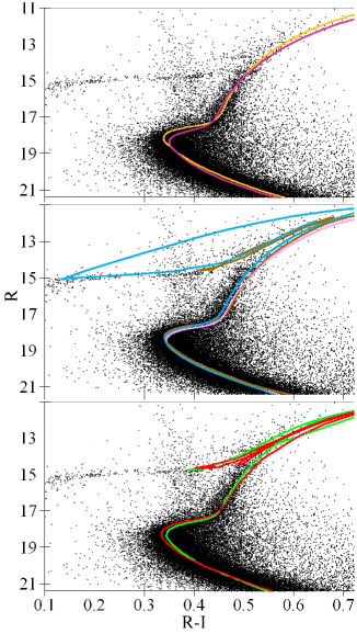
Figure 10: The same as Fig. 6 but for $R-I$ versus $R$.

Some our CMDs can be compared with those presented by Casagrande & VandenBerg (2014, 2018a). They have compared the same HST/ACS, $UBVRI$, Pan-STARRS, and SDSS photometry of NGC 5904 with a set of the Victoria-Regina isochrones. They adopted the reddenings and extinction law from Schlafly & Finkbeiner (2011). In particular, our Fig. 7 can be compared with the figure 10 from Casagrande & VandenBerg (2014), while our Fig. 13 with the figure 7 from Casagrande & VandenBerg (2018a). Usually their isochrones lie about 0.05 mag to the red of the fiducial sequences. In some cases this offset is different for the RGB and MS in the same CMD. To achieve a fully consistent fit (to make the isochrones bluer) one has to adopt an improbable nearly zero reddening, much lower than the adopted estimate $E(B-V)=0.032$ mag from Schlafly & Finkbeiner (2011). Thus, different models/isochrones may be more or less reliable in such a fitting. Consequently, it is clearly advantageous to use different models/isochrones to fit CMDs. Also, it is evident from our results that PARSEC, MIST, DSEP, and BaSTI are quite reliable in this task.

The distance to NGC 5904 is determined better for the models and data for both the HB and TO (PARSEC, MIST, and new BaSTI, which obsoletes old BaSTI). However, we do not use the PARSEC $F275W-F336W$ and $F336W-F438W$ colours with the failed fitting, all the $UBVRI$-WISE colours due to their noisy TO, $H_{\mathrm{UKIDSS}}-W1$ colour due to its poor separation of the HB and TO from the MS, and all SDSS colours due to their large systematic offsets discussed below. The values used to derive the distance are highlighted in Table 3 with bold. By use of them, we calculate the most probable distance to NGC 5904 as $7386\pm 311$ pc, i.e. a true distance modulus of $(m-M)_{0}=14.34\pm 0.09$ mag. The apparent $V$-band distance modulus based on this estimate is compared with the literature in Sect. 5.1.

From our estimate of the distance we calculate the parallax $0.135\pm 0.006$ mas. This agrees with recent estimate of the parallax from the Gaia DR2 $0.113+0.029=0.142\pm 0.040$ mas, where $0.029$ and $0.040$ mas are the parallax global zero-point correction derived from the analysis of the high-precision quasar sample and the median uncertainty in parallax, respectively (Lindegren et al., 2018).

The age might be determined better for models with both the solar-scaled and He-$\alpha$-enhanced abundances (DSEP and old BaSTI) fitted to the data on the SGB. However, we do not use the DSEP $F275W-F336W$ colour with the failed fitting, all the $UBVRI$-WISE colours, the $H_{\mathrm{UKIDSS}}-W1$ colour (its adopted age of 12 Gyr is highlighted in Table 3 with italic), and all the SDSS colours for the same reasons as for the distance. The used values are highlighted in Table 3 with bold. They provide the age $12.15\pm 0.70$ Gyr. This is in line with the age and its uncertainty derived from APM: either 11.2 or 12.6 Gyr. The fitting is almost equally good for both the ages. Therefore, the age can be determined from APM as $11.9\pm 0.7$ Gyr. Yet, we have found in our fitting that the age for NGC 5904 is quite uncertain: its variation by $\pm 1$ Gyr from the best fit gives an almost equally good fitting. Thus, our final estimate of the age is $12.15\pm 1.00$ Gyr. This value agrees well with different estimates from the literature. Few cases outside this range in Table 3 can be explained by an imperfection of the models.

The obtained distance and age values show no dependence on colour. This is not the case for the obtained values of reddening. They must represent a dependence of extinction on wavelength, i.e. an extinction law. Each model and each series of the data gives its own set of extinctions and its own extinction law. Below, we compare them with each other and with the law of CCM89.

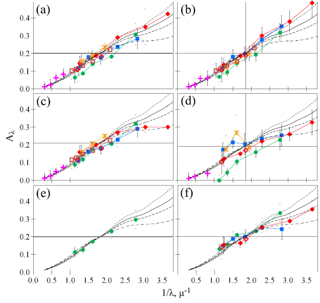
Figure 3: The extinction laws from the isochrone fitting by (a) PARSEC, (b) MIST, (c) DSEP, (d) new BaSTI, (e) APM, and (f) old BaSTI. The HST series – red diamonds (open ones for the WFPC2 data), Gaia series – yellow snowflakes, $UBVRI$ series – blue squares, SDSS series – green circles, Pan-STARRS series – brown squares, and IR series – purple crosses. The black dotted, solid, dashed and dash-dotted black curves show the CCM89 extinction law with $R_{\mathrm{V}}=2.6$, 3.1, 3.6, and 5, respectively.

5.1 Extinction law

PARSEC, MIST, DSEP and new BaSTI, in contrast to APM and old BaSTI, provide us with IR colours. The IR extinction and its variation due to some reasonable variations of the extinction law are very low. For example, $E(B-V)=0.03$ with the CCM89 extinction law with $R_{\mathrm{V}}=3.1$ corresponds to $A_{\mathrm{K_{s}}}=0.012$ and $A_{\mathrm{W1}}=0.006$ mag. Anyway, such values are lower than a typical systematic uncertainty of 0.02 mag for the fitting of the CMDs with the $K_{s}$ and $W1$ colours (see Table 3). Hence, our calculations of the optical and UV extinctions are based on the fact that the IR extinctions used are nearly zero and almost independent of the extinction law.

Namely, given $A_{\mathrm{K_{s}}}=0.012$ and $A_{\mathrm{W1}}=0.006$ mag, we calculate the extinctions for the remaining 27 bands, including $A_{\mathrm{B}}$ and $A_{\mathrm{V}}$, then calculate $R_{\mathrm{V}}=A_{\mathrm{V}}/(A_{\mathrm{B}}-A_{\mathrm{V}})$ and use the CCM89 extinction law with this $R_{\mathrm{V}}$ to re-calculate $A_{\mathrm{K_{s}}}$ and $A_{\mathrm{W1}}$. The iterations of this procedure converge to some extinction values, including $A_{\mathrm{K_{s}}}=0.02$ and $A_{\mathrm{W1}}=0.01$, as well as $A_{\mathrm{V}}=0.20$, 0.20, 0.21 and 0.19 mag for PARSEC, MIST, DSEP, and new BaSTI, respectively, by use of the HST, Gaia, $UBVRI$ and Pan-STARRS data series. These values are shown in Fig. 3 by the black horizontal lines, while the $V$ band – by the black vertical lines. This Figure shows all the derived extinctions as some functions of $1/\lambda$ (i.e. as extinction laws) for the fits by (a) PARSEC, (b) MIST, (c) DSEP, and (d) new BaSTI. The different series of data are shown by different colours. The uncertainties of the extinctions are calculated from the uncertainties of the reddenings and shown in Fig. 3 by the vertical bars. The black curves show the CCM89 extinction law with different $R_{\mathrm{V}}$.

The optical-IR and IR-IR CMDs and the reddenings (isochrone-fiducial colour offsets) derived from them appear the key data in our study. Hence, we note that the extinctions for the five optical data series are based on the derived (i) $E(F814W-K_{s})$, (ii) $E(G-W1)$ and $E(G_{\mathrm{RP}}-W1)$, (iii) $E(I-H_{\mathrm{UKIDSS}})$ and $E(H_{\mathrm{UKIDSS}}-W1)$ [$E(I-W1)$ for new BaSTI], (iv) $E(y_{\mathrm{P1}}-W1)$, and (v) $E(z-K_{s})$ for the HST, Gaia, $UBVRI$, Pan-STARRS, and SDSS series, respectively. Thus, all these extinctions from the five data series by the four models are based on the adopted $A_{\mathrm{K_{s}}}$ or $A_{\mathrm{W1}}$.

Fig. 3 shows a good agreement between the extinction laws from the different models, except the UV bands, as well as between the different data series, except a noticeable negative offset of the SDSS series for all the models. The SDSS photometry may be less accurate than the one from HST, Gaia, $UBVRI$ and Pan-STARRS (see, for example, a discussion on some errors of the SDSS photometry by An et al. 2008; Dotter et al. 2008). Therefore, the SDSS results are not used for calculating the final average values of the extinctions, distance and age.

The average $A_{\mathrm{V}}$ is $0.2$ mag. This is the main result of our study. Its systematic uncertainty is dominated by a systematic uncertainty of about $0.02$ mag of the zero-point IR extinctions $0<A_{\mathrm{K_{s}}}<0.04$ and $0<A_{\mathrm{W1}}<0.02$. These constraints include all possible variations of these extinctions due to any variation of any real or adopted extinction law. Therefore, in fact, $A_{\mathrm{K_{s}}}$, $A_{\mathrm{W1}}$ and all other extinctions, derived by use of PARSEC, MIST, DSEP and new BaSTI, are not tied to the CCM89 or any other extinction law. Therefore they can be used to analyse a real extinction law in the direction of NGC 5904. Fig. 3 shows that all the extinction values, except $A_{\mathrm{F275W}}$ for MIST and some for the SDSS, agree with the CCM89 extinction law with $R_{\mathrm{V}}=3.60\pm 0.05$ (dashed curve) within their precision. Thus, we conclude that the data for NGC 5904 do not need an unusual extinction law.

With the estimate $A_{\mathrm{V}}=0.2$ mag we obtain an apparent $V$-band distance modulus of $(m-M)_{\mathrm{V}}=14.54\pm 0.11$ mag, which includes the additional error inherent in $A_{\mathrm{V}}$. This agrees with $(m-M)_{\mathrm{V}}=14.46$ from Harris (1996) and $14.47\pm 0.07$ from VandenBerg & Denissenkov (2018) obtained as an average of various estimates.

In contrast to PARSEC, MIST, DSEP and new BaSTI, APM and old BaSTI have no IR colour. Hence, their extinctions have to be based on extinction estimates for their reddest bands from CCM89 extinction law with $R_{\mathrm{V}}$ as a free parameter. All their extinction series are reduced to $A_{\mathrm{V}}=0.2$, on average. We derive $R_{\mathrm{V}}=5$ and, hence, $E(B-V)=0.2/5=0.04$ mag for both APM and old BaSTI. Fig. 3 (e), (f) shows the extinctions derived by use of APM and old BaSTI, respectively. Yet, these incomplete results only show that their reddenings in the optical and UV ranges agree with those from PARSEC, MIST, DSEP and new BaSTI, when a zero-point extinction is fixed.

We have found a rather high optical extinction for NGC 5904. It is about twice higher than the ‘canonical’ $A_{\mathrm{V}}=0.09$ mag (as a product of $E(B-V)=0.03$ by $R_{\mathrm{V}}=3.1$) from Harris (1996). This may be related to the well-known issue that a ‘larger reddening than suggested by the adopted reddening curve is needed in some cases [for open and globular clusters]’ (Dotter et al., 2008).

As evident from Fig. 3 and Table 3, this high extinction is due to rather high reddenings between the IR and the optical bands. It is true as for long (such as $G-W1$), as for short (such as $H_{\mathrm{UKIDSS}}-W1$) colour baselines. A lower part of Table 3 with the optical-IR and IR-IR colours shows that the derived reddenings tend to be twice as high as those calculated from Harris’s $E(B-V)=0.03$ mag. Taking into account nearly zero IR extinctions, this means a rather high extinction in the range $625<\lambda<2000$ nm. Indeed, it is seen from Fig. 3 that the slopes of the data series within this range (i.e. $0.5<1/\lambda<1.6$) tend to be steeper than within $1.6<1/\lambda<2.0$, near the $V$ band. Thus, the range $625<\lambda<2000$ nm produces the bulk of the value $A_{\mathrm{V}}=0.2$.

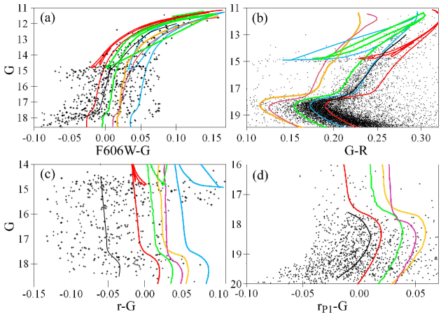
Figure 4: The CMDs of NGC 5904 (a) $F606W-G$ versus $G$, (b) $G-R$ versus $G$, (c) $r-G$ versus $G$, and (d) $r_{\mathrm{P1}}-G$ versus $G$ with the fiducial sequences (black curve) and the isochrones for the age 12 Gyr, distance 7.4 kpc, reddening $E(B-V)=0.03$ mag and CCM89 extinction law with $R_{V}=3.1$, coloured as in Fig. 1.

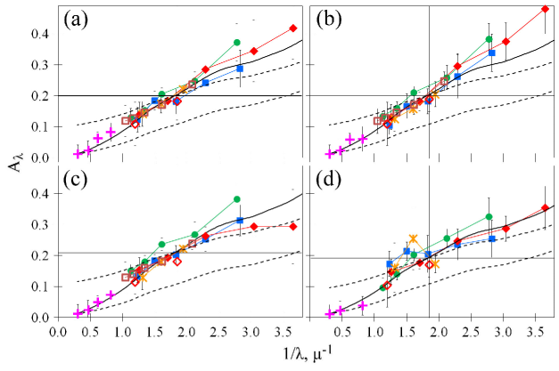
Figure 5: The extinction laws from the isochrone fitting by (a) PARSEC, (b) MIST, (c) DSEP, and (d) new BaSTI after the adjustment for the systematic offsets from Table 5. The designation of the data series as in Fig. 3. The black solid curve shows the CCM89 extinction law with $A_{\mathrm{V}}$ derived for the models and $R_{\mathrm{V}}=3.6$. The black lower dotted curve shows the CCM89 extinction law with $A_{\mathrm{V}}=0.09$ mag and $R_{\mathrm{V}}=3.1$, while the upper one shows the same but shifted up to $A_{\mathrm{V}}$ derived for the models.

6 Discussion

The large offsets of the isochrones from the observations in the optical-IR and IR-IR CMDs may be explained by some inherent offsets of the model colours by about 0.1 mag, similar for all models, as well as for all colours, which are close to each other.

Moreover, such inherent offsets of the model colours, being different for different data series, may explain the vertical offsets (i.e. the different extinction laws) of the data series, which are seen in Fig. 3.

To test these assumptions, we analyse some CMDs with rather close colour bands, which have a difference of their extinction coefficients $<0.2$. In this case, any reasonable variation of the extinction and reddening (e.g. within $0.02<E(B-V)<0.12$ mag) does not shift any isochrone in this CMD along the colour by more than $0.2\times(0.12-0.02)=0.02$ mag. This is negligible w.r.t. the colour offsets under consideration. It appears that any reasonable variation of [Fe/H], abundance, age, and distance also does not shift these isochrones by more than 0.02 mag. This means that any considerable colour offset between an isochrone and the fiducial sequence in such a CMD is due to an imperfection of this isochrone.

A quite interesting range, $588<\lambda_{\mathrm{eff}}<667$ nm, contains 5 close bands: $F606W$, $G$, $r$, $R$ and $r_{\mathrm{P1}}$ (see Table 1). We consider only their colours with the extinction coefficients $<0.2$. Four CMDs with such colours, together with the isochrones from PARSEC, MIST, DSEP, and new BaSTI for the age 12 Gyr, distance 7.4 kpc, $E(B-V)=0.03$ and CCM89 extinction law with $R_{V}=3.1$ are presented in Fig. 4. All the CMDs show offsets of the isochrones from the fiducial sequences (black curves) within $\pm 0.05$ mag, except those with the SDSS $r$ band with some offsets up to 0.11 mag. These offsets are different for different models/isochrones in the same CMD, as well as for different series/colours. This is explained, among other reasons, by quite different colour-$T_{\mathrm{eff}}$ relations and bolometric corrections in these models, as discussed by Paxton et al. (2011); Choi et al. (2016); Hidalgo et al. (2018). Therefore, Fig. 4 shows that the situation when the four models (PARSEC, MIST, DSEP and new BaSTI) provide by chance the same inherent optical-IR colour offsets of about 0.1 mag for the four data series (HST, Gaia, Pan-STARRS and $UBVRI$) is quite unlikely. It is even more unlikely that some large inherent colour offsets for the bands, at least, from $F438W$ to $K_{s}$, i.e. within $430<\lambda<2200$ nm, precisely follow by chance the CCM89 extinction law [i.e. provide the small scatter of the symbols around a black curve in Fig. 3 (a)–(d)]. Hence, the discovered optical-IR colour offsets seem to be not inherent, but generated by reddening.

Moreover, the comparison of the MIST, PARSEC, DSEP and BaSTI isochrones in the plane of luminocity versus T_eff for $Z=0.0001$ and age 10 Gyr, i.e. for typical parameters for GCs, by Choi et al. (2016) (see their figure 16) shows that for the same luminocity a difference in T_eff is always within $\pm 150$ K. This corresponds to $\pm 0.03$ mag of a colour offset [see VandenBerg & Denissenkov (2018)]. This is much less than the colour offset of about 0.1 mag, which needs to be explained. Figure 18 of Choi et al. (2016) confirms this: for an age of 10 Gyr any difference between the MIST, PARSEC and BaSTI optical-IR and IR-IR colours (even for $V-K$) is much less than 0.1 mag. However, Kucinskas et al. (2006), Hendricks et al. (2012) have found that an uncertainty of T_eff of 100 K can lead to an uncertainty of the optical-IR colours of the RGB and AGB stars up to 0.05 mag. This is another reason why we have paid more attention to the TO, SGB, MS than to the RGB and AGB in our isochrone fitting. Finally, we are inclined to conclude with a caution that the large derived colour offsets between the isochrones and the fiducial sequences in the optical-IR and IR-IR CMDs are due to extinction rather than to inherent model colour offsets.

Table 5: The offset correrctions (mag) applied for the various data series and models.

Model

Series PARSEC MIST DSEP new BaSTI

HST $$-0.005$$ 0.026

Gaia 0.005

0.005 0.022

Pan-STARRS 0.015 0.015 0.012

SDSS 0.065 0.065 0.062 0.096

To explain the difference between the extinction laws for the different data series in Fig. 3, we adjust the colour offsets from Fig. 4 assuming the means of the HST, Gaia, $UBVRI$ and Pan-STARRS extinctions as true and, hence, fixing them. This gives us some constant corrections to the extinction laws for the various data series and models, which are presented in Table 5. These corrections, except for SDSS, are nearly zero. This means that the inter-series CMDs (such as in Fig. 4) and their reddenings are in line with the intra-series CMDs (as in Fig. 1–2 and 6–15) and their reddenings. This, in turn, means that the series agree with each other.

The extinction laws from PARSEC, MIST, DSEP, and new BaSTI with these corrections applied are shown in Fig. 5, which is similar to Fig. 3. This adjustment decreases the scatter of the data series, except the SDSS.

The black solid curve in Fig. 5 shows the CCM89 extinction law with $R_{\mathrm{V}}=3.6$ and with $A_{\mathrm{V}}$ derived for the models. As in Fig. 3, it is seen that all the extinctions, except $A_{\mathrm{F275W}}$ for MIST and some for the SDSS, agree with this law within their precision.

The black dotted curves in Fig. 5 show the CCM89 extinction law with $R_{\mathrm{V}}=3.1$ for $A_{\mathrm{V}}=0.09$ mag (lower curve) and $A_{\mathrm{V}}$ derived for the models (upper curve). Thus, the lower curve extrapolates the Harris’s value of $E(B-V)=0.03$ mag out of the range between the $B$ and $V$ bands. The upper curve is drawn to emphasise that all the data series, including also the HST WFPC2 (the red open diamonds), being scarcely agreed with $E(B-V)=0.03$ mag (the slope of the upper dotted curve), yet, demonstrate a steeper slope (i.e. $E(B-V)>0.03$ mag), which better agrees with the slope of the solid curve (i.e. $E(B-V)=0.055$ mag). This is a very important result, since the reddenings derived in our fits (i.e. the slopes of the series in the Fig. 3 and 5) are independent of any zero-point extinction. In other words, these steep slopes and a positive minimal extinction are the only reasons for such a high $A_{\mathrm{V}}$.

The reddenings for the long-baseline colours [such as $E(F438W-W1)$] obtained by us show a good agreement with the CCM89 extinction law with $R_{\mathrm{V}}=3.6$ and $A_{\mathrm{V}}=0.2$ mag. However, some reddenings for the short-baseline colours from Table 3 (such as $E(H_{\mathrm{UKIDSS}}-W1)$) show some noticeable small-scale deviations from this law. These deviations may explain the diversity of the reddening estimates discussed in Sect. 1. On the one hand, Table 3 gives us the average $E(B-V)=0.054\pm 0.020$ mag in a good agreement with the CCM89 extinction law giving $E(B-V)=A_{\mathrm{V}}/R_{\mathrm{V}}=0.2/3.6=0.056$ mag. Given its uncertainty of $\pm 0.02$ mag, this estimate is in the best agreement with the one from Green et al. (2018), in a moderate agreement with those of Drimmel, Cabrera-Lavers & López-Corredoira (2003) and SFD, and in a poor agreement with the remaining reddening estimates discussed in Sect. 1, including the Harris’s $E(B-V)=0.03$ mag. On the other hand, Table 3 gives us the averages $E(V-R)=0.007\pm 0.02$ and $E(H_{\mathrm{UKIDSS}}-W1)=0.045\pm 0.01$ mag. With the extinction coefficients $E(V-R)/E(B-V)=0.67$ and $E(H_{\mathrm{UKIDSS}}-W1)/E(B-V)=0.468$ from the CCM89 extinction law with $R_{\mathrm{V}}=3.6$, this gives us $E(B-V)=0.01\pm 0.03$ and $0.10\pm 0.02$ mag, respectively. These values are completely inconsistent with each other. The former and the latter agree best with the lowest reddening estimates from Green et al. (2015) and Arenou, Grenon & Gomez (1992) and the highest ones from Gontcharov (2012b) and Gontcharov (2017), respectively.

Thus, as assumed in Sect. 1, some deviations of the real extinction law from CCM89 may explain the diversity of the previous reddening estimates for NGC 5904, which are inter- or extrapolated by use of a ‘standard’ extinction law from some observations at very different wavelengths.

Fortunately, we have found a real extinction law for NGC 5904 rather close to the CCM89 with a reasonable value of $R_{\mathrm{V}}$. However, it may not be the case for other GCs, which we intend to consider in our future studies.

Our findings are in line with the earlier criticism of the CCM89 extinction law with $R_{\mathrm{V}}=3.1$ as the ‘standard’ and universal one. Some disadvantages of the CCM89 extinction law and the procedure of its creation are well-known (Maíz Apellániz et al., 2014). For example, Fitzpatrick & Massa (2007) have found that there is no strong correlation between the UV and IR Galactic extinctions, in opposition to what CCM89 found. Some different extinction laws with a higher IR extinction, with $R_{\mathrm{V}}>3.1$, and with a grey extinction are typical far from the Galactic mid-plane (NGC 5904 is about 5.5 kpc above the mid-plane) instead of the CCM89 extinction law (Gorbikov & Brosch, 2010; Gontcharov, 2012a; Hendricks et al., 2012; Gontcharov, 2013; Davenport et al., 2014; Gontcharov, 2016a, b). Moreover, (Hendricks et al., 2012) have found $R_{\mathrm{V}}=3.62\pm 0.07$ in the line of sight to the GC M4 as a result of a study, similar to ours. An excellent agreement of this result with our $R_{\mathrm{V}}=3.60\pm 0.05$ for NGC 5904 (M5) may be explained. M4 and NGC 5904 are in the same sky area affected by a higher extinction and unusual extinction law at the upper part of the Gould Belt (near $l\approx 15\degr$, $b\approx+19\degr$) (Gontcharov, 2009, 2012a, 2016b). ‘We find that dust at high latitude is neither quantitatively nor qualitatively consistent with standard reddening laws.’ (Peek & Schiminovich, 2013).

7 Conclusions

In this study we have tested the expectation that an accurate fitting of the isochrones to a multi-band photometry for a GC can provide some convergent estimates of its distance and age, together with a set of estimates of the interstellar extinction in dependence on wavelength. This set represents the real extinction law to the cluster. We used the photometry of NGC 5904 (M5) in 29 bands from the HST, WISE, Gaia DR2, SDSS, UKIDSS, NTT, TNG, Pan-STARRS, and a compilation of the $UBVRI$ photometry. These bands cover a wavelength range from about 235 to 4070 nm, i.e. from the UV to mid-IR. To fit the data, we used the following five theoretical models of the stellar evolution: PARSEC, MIST, DSEP, BaSTI (the old and new version), and the model from An et al. (2009). Some of the isochrones, which they produce, are calculated for non-scaled-solar abundances, with enhanced He and $\alpha$-elements. Yet, the fitting revealed that for NGC 5904 the difference between scaled-solar and non-scaled-solar isochrones is quite small, and both kinds of isochrones can be used. We accept a metallicity of about [Fe/H]$=-1.33$ based on the spectroscopy taken from the literature.

We found for NGC 5904 the age to be $12.15\pm 1$ Gyr, distance $7386\pm 311$ pc, true distance modulus $(m-M)_{0}=14.34\pm 0.09$ and apparent $V$-band distance modulus $(m-M)_{\mathrm{V}}=14.54\pm 0.11$. These estimates agree with the literature estimates including the recent one from Gaia DR2 $0.113+0.029=0.142$ mas, where $+0.029$ mas is the well-established global zero-point correction (Lindegren et al., 2018).

From the fitting we found some systematic colour offsets of the isochrones from the fiducial sequences in the CMDs. These offsets draw some monotonic functions of colour. Hence, they can be interpretted as sets of the extinctions drawing an extinction law for each data series. Nearly zero extinctions in $K_{s}$ and $W1$ bands, which are almost independent of extinction law, are used as zero-point extinctions in the HST, Gaia, Pan-STARRS, $UBVRI$, and SDSS data series in their fitting by PARSEC, MIST, DSEP, and new BaSTI. As the main result of our study, all the extinction laws derived in the fitting of these data series, except the SDSS, by these four models agree with each other and with the CCM89 extinction law with $R_{\mathrm{V}}=3.6$ and $A_{\mathrm{V}}=0.20\pm 0.02$ mag. This uncertainty includes the uncertainties of the zero-point IR extinctions, of the extinction law, as well as the scatter of the results of the fittings of the four data series by the four models. Old BaSTI and the model from An et al. (2009), providing no IR colour, cannot draw a complete extinction law. Yet, their reddenings in the optical range do not contradict the remaining models.

All the data and models show agreed deviations from the CCM89 extinction law with $R_{\mathrm{V}}=3.6$ for some short-baseline colours, such as $V-R$ and $H_{\mathrm{UKIDSS}}-W1$. These deviations can explain the diversity of the previous reddening estimates for NGC 5904, which were inter- or extrapolated by use of a ‘standard’ extinction law from some observations at very different wavelengths.

The obtained $E(B-V)=0.054\pm 0.020$ is in a moderate agreement with the generally accepted $E(B-V)=0.03$ from Harris (1996) and with the set of non-independent estimates of $E(B-V)\approx 0.35$ from Meisner & Finkbeiner (2015), Schlafly & Finkbeiner (2011), Drimmel, Cabrera-Lavers & López-Corredoira (2003), Lallement et al. (2018), and SFD within their uncertainties. However, due to the rather high $R_{\mathrm{V}}=3.6$, the obtained $A_{\mathrm{V}}=0.2$ mag is nearly twice as high as the generally accepted $A_{\mathrm{V}}=0.09$ mag, as the product of $E(B-V)=0.03$ by $R_{\mathrm{V}}=3.1$. A bulk of the extinction $A_{\mathrm{V}}=0.2$ mag appears within $625<\lambda<2000$ nm. Hence, the extinction in this range cannot be reconciled with $R_{\mathrm{V}}=3.1$.

However, the obtained large colour offsets between the isochrones and the fiducial sequences in the CMDs may also include some inherent offsets of model colours, e.g. due to some errors of the colour-$T_{\mathrm{eff}}$ calibrations used. Yet, such a large inherent colour offset of about 0.1 mag, similar in the fitting of the four independent data series by the four rather different models seems to be rather unlikely. Thus, we are inclined to conclude that a real extinction law for the dust medium between us and NGC 5904 is close to the CCM89 extinction law with $R_{\mathrm{V}}=3.6$ and $A_{\mathrm{V}}=0.2$ mag. Nevertheless, a further improvement of the theoretical models and isochrones is highly needed.

Appendix A Some CMDs of NGC 5904

Figure 8: The same as Fig. 6 but for $F555W-F814W$ versus $F555W$.

Figure 9: The same as Fig. 6 but for $G_{\mathrm{BP}}-G_{\mathrm{RP}}$ versus $G$.

Figure 12: The same as Fig. 6 but for $J-K_{s}$ versus $K_{s}$.

Figure 13: Pan-STARRS $g_{P1}-r_{P1}$ versus $r_{P1}$ CMD of NGC 5904 with the fiducial sequence from Bernard et al. (2014) – the black thick curve, and the isochrones coloured as in Fig. 6 with the best-fit parameters from Table 3.

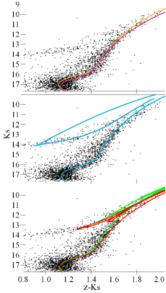
Figure 15: The same as Fig. 6 but for $z-K_{s}$ versus $K_{s}$.

References

- An et al. (2008) An D. et al., 2008, ApJS, 179, 326
- An et al. (2009) An D. et al., 2009, ApJ, 700, 523 (APM)