AABI 20181st Symposium on Advances in Approximate Bayesian Inference, 2018

Non-Factorised Variational Inference in Dynamical Systems

1 Introduction

Many real world systems exhibit complex non-linear dynamics, and a wide variety of approaches have been proposed to model them. Characterising these dynamics is essential to the analysis of a system’s behaviour, as well as to prediction. Autoregressive models map past observations to future ones and are very common in diverse fields such as economics and model predictive control. State-space models (SSMs), lift the dynamics from the observations to a set of auxiliary, unobserved variables (the latent states $\{\mathbf{x}_{t}\}_{t=1}^{T}$) which fully describe the state of the system at each time-step, and thus take the system to evolve as a Markov chain. The “transition function” maps a latent state to the next. We place a Gaussian process (GP) prior on the transition function, obtaining the Gaussian process state-space model (GPSSM). This Bayesian non-parametric approach allows us to: 1) obtain uncertainty estimates and predictions from the posterior over the transition function, 2) handle increasing amounts of data without the model saturating, and 3) maintain high uncertainty estimates in regions with little data.

While many approximate inference schemes have been proposed (Frigola et al., 2013), we focus on variational “inducing point” approximations (Titsias, 2009), as they offer a particularly elegant framework for approximating GP models without losing key properties of the non-parametric model. Since a non-parametric Gaussian process is used as the approximate posterior (Matthews et al., 2016), the properties of the original model are maintained. Increasing the number of inducing points, we add capacity to the approximation, and the quality of the approximation is measured by the marginal likelihood lower bound (or evidence lower bound – ELBO).

The accuracy of variational methods is fundamentally limited by the class of approximate posteriors, with independence assumptions being particularly harmful for time-series models (Turner et al., 2010). Several variational inference schemes that factorise the states and transition function in the approximate posterior have been proposed (Frigola et al., 2014; McHutchon et al., 2014; Ialongo et al., 2017; Eleftheriadis et al., 2017). Here, we investigate the design choices which are available in specifying a non-factorised posterior.

2 Gaussian Process State Space Models

Conceptually, a GPSSM is identical to other SSMs. We model discrete-time sequences of observations $\mathbf{Y}=\mathopen{}\mathclose{{}\left\{\mathbf{y}_{t}}\right\}_{t=1}^{T}$, where $\mathbf{y}_{t}\in\mathbb{R}^{E}$, by a corresponding latent Markov chain of states $\mathbf{X}=\mathopen{}\mathclose{{}\left\{\mathbf{x}_{t}}\right\}_{t=1}^{T}$ where $\mathbf{x}_{t}\in\mathbb{R}^{D}$. All state-to-state transitions are governed by the same transition function $f$. For simplicity, we take the transition $p(\mathbf{x}_{t+1}\,|\,f,\mathbf{x}_{t})$ and observation $p(\mathbf{y}_{t}\,|\,\mathbf{x}_{t})$ densities to be Gaussians, although any closed form density function could be chosen. Without loss of generality (subject to a suitable augmentation of the state-space) (Frigola, 2015), we also assume a linear mapping between $\mathbf{x}_{t}$ and the mean of $\mathbf{y}_{t}\,|\,\mathbf{x}_{t}$ to alleviate non-identifiabilities between transitions and emissions. The generative model is specified by the following equations:

$$\begin{aligned} f&\sim\mathcal{GP}(0,k(\cdot,\cdot))\,\\ \mathbf{x}_{t+1}\,|\,f,\mathbf{x}_{t}&\sim\mathcal{N}\mathopen{}\mathclose{{}\left({f(\mathbf{x}_{t}),\mathbf{Q}}}\right)\,\\ \end{aligned}\qquad\qquad\begin{aligned} \mathbf{x}_{1}&\sim\mathcal{N}\mathopen{}\mathclose{{}\left({\mathbf{0},\mathbf{I}}}\right)\,\\ \mathbf{y}_{t}\,|\,\mathbf{x}_{t}&\sim\mathcal{N}\mathopen{}\mathclose{{}\left({\mathbf{C}\mathbf{x}_{t}+\mathbf{d},\mathbf{R}}}\right)\,\\ \end{aligned}$$ (1)

the function values $f(\mathbf{x}_{t})$ are given by the GP as:

$$f(\mathbf{x}_{t})\,|\,\mathbf{x}_{1:t},f(\mathbf{x}_{1:t-1})\sim\mathcal{N}\mathopen{}\mathclose{{}\left({\bm{\mu}_{f_{t}},\mathbf{C}_{f_{t}}}}\right)\qquad\qquad\quad f(\mathbf{x}_{1:t-1})\triangleq\mathopen{}\mathclose{{}\left[f(\mathbf{x}_{1})^{\top},\dots,f(\mathbf{x}_{t-1})^{\top}}\right]^{\top}$$ (2)

$$\bm{\mu}_{f_{t}}\triangleq K_{\mathbf{x}_{t},\mathbf{x}_{1:t-1}}K_{\mathbf{x}_{1:t-1},\mathbf{x}_{1:t-1}}^{-1}f(\mathbf{x}_{1:t-1})\qquad\mathbf{C}_{f_{t}}\triangleq K_{\mathbf{x}_{t},\mathbf{x}_{t}}-K_{\mathbf{x}_{t},\mathbf{x}_{1:t-1}}K_{\mathbf{x}_{1:t-1},\mathbf{x}_{1:t-1}}^{-1}K_{\mathbf{x}_{1:t-1},\mathbf{x}_{t}}$$

3 Design choices in variational inference

We want a variational approximation to $p(\mathbf{X},f\,|\,\mathbf{Y})$. We begin by writing our approximate posterior as $q(\mathbf{X},f)=q(\mathbf{X}\,|\,f)q(f)$ For $q(f)$ we choose an inducing point posterior according to Titsias (2009) and Hensman et al. (2013) and write $q(f)=p(f^{\setminus\mathbf{u}}\,|\,\mathbf{u})q(\mathbf{u})$ by splitting up the function into the inducing outputs $\mathbf{u}$ and all other points $f^{\setminus\mathbf{u}}$. For our $q(\mathbf{X}\,|\,f)$, we will consider Markovian distributions, following the structure of the exact posterior:

$$q(\mathbf{X}\,|\,f)=q(\mathbf{x}_{1})\prod_{t=1}^{T-1}q(\mathbf{x}_{t+1}\,|\,f,\mathbf{x}_{t})$$ (3)

This allows us to write down the general form of the variational lower bound:

$$\log p(\mathbf{Y})\geq\int q(f,\mathbf{X})\log\Bigg{[}\frac{p(f^{\setminus\mathbf{u}}\,|\,\mathbf{u})p(\mathbf{u})p(\mathbf{x}_{1})\prod_{t=1}^{T-1}p(\mathbf{x}_{t+1}\,|\,f,\mathbf{x}_{t})}{p(f^{\setminus\mathbf{u}}\,|\,\mathbf{u})q(\mathbf{u})q(\mathbf{x}_{1})\prod_{t=1}^{T-1}q(\mathbf{x}_{t+1}\,|\,f,\mathbf{x}_{t})}\prod_{t=1}^{T}p(\mathbf{y}_{t}\,|\,\mathbf{x}_{t})\Bigg{]}\mathrm{d}f\mathrm{d}\mathbf{X}$$ (4)

$$\phantom{\log p(\mathbf{Y})\,}=\sum_{t=1}^{T}\mathbb{E}_{q(\mathbf{x}_{t})}\mathopen{}\mathclose{{}\left[\log p(\mathbf{y}_{t}\,|\,\mathbf{x}_{t})}\right]-\mathrm{KL}\mathopen{}\mathclose{{}\left[\,q(\mathbf{u})\,\middle\|\,p(\mathbf{u})\,}\right]-\mathrm{KL}\mathopen{}\mathclose{{}\left[\,q(\mathbf{x}_{1})\,\middle\|\,p(\mathbf{x}_{1})\,}\right]$$

$$\phantom{\log p(\mathbf{Y})\geq}\qquad\qquad-\sum_{t=1}^{T-1}\mathbb{E}_{q(f,\mathbf{x}_{t})}\mathopen{}\mathclose{{}\left[\mathrm{KL}\mathopen{}\mathclose{{}\left[\,q(\mathbf{x}_{t+1}\,|\,f,\mathbf{x}_{t})\,\middle\|\,p(\mathbf{x}_{t+1}\,|\,f,\mathbf{x}_{t}))\,}\right]}\right]$$ (5)

We are now left to specify the form of $q(\mathbf{x}_{1})$, $q(\mathbf{u})$, and $q(\mathbf{x}_{t+1}\,|\,f,\mathbf{x}_{t})$. For the first two, we choose Gaussian distributions and optimise variationally their means and covariances, while, for the last, several choices are available. We follow the form of the exact filtering distribution (for Gaussian emissions) but treat $\and,\mathbf{b}_{t},\mathbf{S}_{t}$ as free variational parameters to be optimised (thus approximating the smoothing distribution):

$$q(\mathbf{x}_{t+1}\,|\,f,\mathbf{x}_{t})=\mathcal{N}\mathopen{}\mathclose{{}\left({\mathbf{x}_{t+1}\,|\,\and\mathbf{f}_{t}+\mathbf{b}_{t},\mathbf{S}_{t}^{*}}}\right)$$ (6)

	$q(\mathbf{X}\,|\,f)$	$\mathbf{f}_{t}$	$\mathbf{S}_{t}^{*}$	sampling
1) Factorised - linear	$q(\mathbf{X})$	$\mathbf{x}_{t}$	$\mathbf{S}_{t}$	$\mathcal{O}(T)$
2) Factorised - non-linear	$q(\mathbf{X})$	$K_{\mathbf{x}_{t},\mathbf{Z}}K_{\mathbf{Z},\mathbf{Z}}^{-1}\bm{\mu}_{\mathbf{u}}$	$\mathbf{S}_{t}+\and\mathbf{C}_{f}(\mathbf{x}_{t})\and^{\top}$	$\mathcal{O}(T)$
3) U-Factorised - non-linear	$q(\mathbf{X}\,|\,\mathbf{u})$	$K_{\mathbf{x}_{t},\mathbf{Z}}K_{\mathbf{Z},\mathbf{Z}}^{-1}\mathbf{u}$	$\mathbf{S}_{t}+\and\mathbf{C}_{f|\mathbf{u}}(\mathbf{x}_{t})\and^{\top}$	$\mathcal{O}(T)$
4) Non-Factorised - non-linear	$q(\mathbf{X}\,|\,f)$	$f(\mathbf{x}_{t})$	$\mathbf{S}_{t}$	$\mathcal{O}(T^{3})$

Table 1: Variations of approximate posteriors. $\and,\mathbf{b}_{t},\mathbf{S}_{t}$ are free parameters in all cases. $\mathbf{C}_{f}(\mathbf{x}_{t})$ is the sparse GP’s marginal posterior variance:

$$\mathbf{C}_{f}(\mathbf{x}_{t})\triangleq K_{\mathbf{x}_{t},\mathbf{x}_{t}}+K_{\mathbf{x}_{t},\mathbf{Z}}K_{\mathbf{Z},\mathbf{Z}}^{-1}\mathopen{}\mathclose{{}\left(\mathbf{\Sigma}_{\mathbf{u}}-K_{\mathbf{Z},\mathbf{Z}}}\right)K_{\mathbf{Z},\mathbf{Z}}^{-1}K_{\mathbf{Z},\mathbf{x}_{t}}$$

whereas $\mathbf{C}_{f|\mathbf{u}}(\mathbf{x}_{t})$ is the conditional variance of $f(\mathbf{x}_{t})\,|\,\mathbf{u}$:

$$\mathbf{C}_{f|\mathbf{u}}(\mathbf{x}_{t})\triangleq K_{\mathbf{x}_{t},\mathbf{x}_{t}}-K_{\mathbf{x}_{t},\mathbf{Z}}K_{\mathbf{Z},\mathbf{Z}}^{-1}K_{\mathbf{Z},\mathbf{x}_{t}}$$

Each posterior is identified by whether it factorises the distribution between states and transition function, and by whether it is linear in the latent states (i.e. only the first one, which corresponds to a joint Gaussian over the states). The cubic sampling cost associated with the last choice of posterior (“Non-Factorised - non-linear”, i.e. the full GP) derives from having to condition, at every time-step, on a sub-sequence of length $t\in\{0,\dots,T-1\}$, giving $T$ operations, each of $\mathcal{O}(t^{2})$ complexity (i.e. updating and solving a $t\times t$ triangular linear system represented by a Cholesky decomposition). The cost of sampling is crucial, because evaluating and optimising our variational bound requires obtaining samples of $q(\mathbf{x}_{t})$ and $q(f,\mathbf{x}_{t})$ to compute expectations by Monte Carlo integration. We now review two options to side-step the cubic cost associated with the fully non-parametric GP.

3.1 Dependence on the entire process $f$ - “Chunking”

If we wish to retain the full GP as well as a non-factorised posterior, but the data does not come in short independent sequences, one approach is to “cut” the posterior $q(\mathbf{X}|f)$ into sub-sequences of lengths $\tau_{1},\dots,\tau_{n}$:

$$q(\mathbf{X}\,|\,f)=\mathopen{}\mathclose{{}\left[q(\mathbf{x}_{1})\prod_{t=1}^{\tau_{1}-1}q(\mathbf{x}_{t+1}\,|\,f,\mathbf{x}_{t})}\right]\mathopen{}\mathclose{{}\left[q(\mathbf{x}_{\tau_{1}+1})\prod_{t=\tau_{1}+1}^{\tau_{1}+\tau_{2}-1}q(\mathbf{x}_{t+1}\,|\,f,\mathbf{x}_{t})}\right]\dots\Bigg{[}\dots\Bigg{]}\,$$ (7)

for $\tau_{1}=\dots=\tau_{n}=\tau$ this reduces the cost of sampling to $\mathcal{O}\mathopen{}\mathclose{{}\left(\frac{T}{\tau}\tau^{3}}\right)$. Conditioning (which has cubic cost in the size of the conditioning set) now only needs to extend as far back as the beginning of the current chunk, where the marginal $q(\mathbf{x}_{i})$ is explicitly represented and can be sampled directly. Moreover we can now “minibatch” over different chunks, evaluating our bound in a “doubly stochastic” manner (Salimbeni and Deisenroth, 2017).

3.2 Dependence on the inducing points $\mathbf{u}$ only - “U-Factorisation”

In order to avoid “cutting” long-ranging temporal dependences in our data by “chunking”, we could instead use the inducing points to represent the dependence between $\mathbf{X}$ and $f$. We can take $q(\mathbf{X}\,|\,f)=q(\mathbf{X}\,|\,\mathbf{u})$ and, constraining $q(\mathbf{X}\,|\,\mathbf{u})$ to be Markovian (which is not exact in general, but is required for efficiency), we write:

$$q(\mathbf{x}_{t+1}\,|\,\mathbf{u},\mathbf{x}_{t})=\mathcal{N}\mathopen{}\mathclose{{}\left({\mathbf{x}_{t+1}\,|\,\and K_{\mathbf{x}_{t},\mathbf{Z}}K_{\mathbf{Z},\mathbf{Z}}^{-1}\mathbf{u}+\mathbf{b}_{t},\mathbf{S}_{t}+\and\mathbf{C}_{f|\mathbf{u}}(\mathbf{x}_{t})\and^{\top}}}\right)$$ (8)

The intuition behind this choice of posterior (corresponding to the third one in the table) is to represent the GP with samples from the inducing point variational distribution (each sample effectively being a different transition function), and to generate trajectories $\mathbf{X}$ for each of the samples. Because these functions are represented parametrically (with finite “resolution” corresponding to the number of inducing points), and our posterior is Markovian, our sampling complexity does not grow as we traverse the latent chain $\mathbf{X}$. If we were to “integrate out” $\mathbf{u}$ (as in the second posterior in the table), however, the dependence between $\mathbf{X}$ and $f$ would be severed (recall $\mathbf{u}$ is “part” of $f$).

4 Experiments

In order to test the effect of the factorisation on the approximate GP posterior (i.e. the learned dynamics), we perform inference on data generated by the “kink” transition function (see Figure 1’s “true function”). The models whose fit is shown are “Factorised - non-linear” and “U-Factorised - non-linear”, both using an RBF kernel. Factorisation leads to an overconfident, mis-calibrated posterior and this is the same for both factorised models (they gave virtually the same fit). Using 100 inducing points, the U-Factorised and Non-Factorised posteriors were also indistinguishable, the transition function being precisely “pinned-down” by the inducing points.

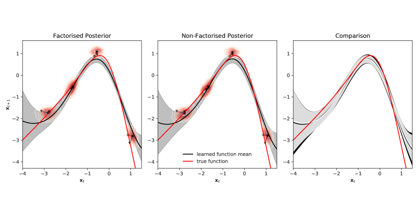
Figure 1: Uncertainty shrinking due to factorisation. Left: fit for the factorised $q(\mathbf{X})q(f)$; Middle: fit for the U-Factorised $q(\mathbf{X}\,|\,\mathbf{u})q(f)$; Right: superimposed posteriors (grey is factorised, black is U-Factorised). All subplots: the shaded regions indicate a $2\sigma$ confidence interval and the contour plots (left and middle) show the pairwise posteriors $q(\mathbf{x}_{t},\mathbf{x}_{t+1})$ over some test latent states. The $(x,y)$ coordinates of the squares, triangles and circles correspond to, respectively: the true latent states $(\mathbf{x}_{t},\mathbf{x}_{t+1})$, the observed states $(\mathbf{y}_{t},\mathbf{y}_{t+1})$ and the means of the marginal posteriors $(\mathbb{E}_{q(\mathbf{x}_{t})}\mathopen{}\mathclose{{}\left[\mathbf{x}_{t}}\right],\mathbb{E}_{q(\mathbf{x}_{t+1})}\mathopen{}\mathclose{{}\left[\mathbf{x}_{t+1}}\right])$.

Appendix A Comparison to PR-SSM

Doerr et al. (2018) were, to the best of our knowledge, the first to consider a non-factorised variational posterior for the GPSSM. Their work, however, has two significant shortcomings. Firstly, the $q(\mathbf{x}_{t+1}|f,\mathbf{x}_{t})$ terms are set to be the same as the corresponding prior terms (i.e. the prior transitions). This posterior fails to exploit information contained in the observations other than by adapting $q(\mathbf{u})$ (it performs no filtering or smoothing on the latent states), and can only be an adequate approximation when the process noise is low and the observed sequence is short (as even low noise levels can compound, and potentially be amplified, in a long sequence). Of course, it would also be an appropriate choice (if somewhat difficult to optimise) when the process noise is zero, but then the latent variables become deterministic, given the transition function, and it is unclear whether modelling them explicitly through a probabilistic state-space model should be beneficial (an auto-regressive model with no latent variables might be sufficient).
Secondly, Doerr et al. (2018) employ a sampling scheme which gives incorrect marginal samples of $q(\mathbf{x}_{t})$, even assuming, as they did, that:

$$p(f(\mathbf{x}_{1}),\dots,f(\mathbf{x}_{T-1})|\mathbf{u})=\prod_{t=1}^{T-1}p(f(\mathbf{x}_{t})|\mathbf{u})$$ (9)

The mistake is predicated on believing that the factorisation in equation 9 produces a Markovian $q(\mathbf{X})$. In general, this is not the case. A mismatch is thus introduced between the form of the variational lower bound and the samples being used to evaluate it, resulting in a spurious objective.

References

- Doerr et al. (2018) Andreas Doerr, Christian Daniel, Martin Schiegg, Duy Nguyen-Tuong, Stefan Schaal, Marc Toussaint, and Sebastian Trimpe. Probabilistic recurrent state-space models. In Proceedings of the 35th International Conference on Machine Learning, 2018.
- Eleftheriadis et al. (2017) Stefanos Eleftheriadis, Tom Nicholson, Marc Deisenroth, and James Hensman. Identification of gaussian process state space models. In Advances in Neural Information Processing Systems 30, 2017. URL http://papers.nips.cc/paper/7115-identification-of-gaussian-process-state-space-models.pdf.
- Frigola (2015) Roger Frigola. Bayesian time series learning with gaussian processes. University of Cambridge, 2015.
- Frigola et al. (2013) Roger Frigola, Fredrik Lindsten, Thomas B. Schön, and Carl E. Rasmussen. Bayesian inference and learning in Gaussian process state-space models with particle MCMC. In Advances in Neural Information Processing Systems 26, 2013. URL http://media.nips.cc/nipsbooks/nipspapers/paper_files/nips26/1449.pdf.
- Frigola et al. (2014) Roger Frigola, Yutian Chen, and Carl Edward Rasmussen. Variational gaussian process state-space models. In Advances in Neural Information Processing Systems 27, 2014. URL http://papers.nips.cc/paper/5375-variational-gaussian-process-state-space-models.pdf.
- Hensman et al. (2013) James Hensman, Nicolo Fusi, and Neil D Lawrence. Gaussian Processes for Big Data. Uncertainty in Artificial Intelligence, 2013.
- Ialongo et al. (2017) Alessandro Davide Ialongo, Mark van der Wilk, and Carl Edward Rasmussen. Closed-form inference and prediction in Gaussian process state-space models. NIPS 2017 Time-Series Workshop, 2017.
- Matthews et al. (2016) Alexander Matthews, James Hensman, Richard Turner, and Zoubin Ghahramani. On sparse variational methods and the kullback-leibler divergence between stochastic processes. In Proceedings of the 19th International Conference on Artificial Intelligence and Statistics, 2016.
- McHutchon et al. (2014) Andrew McHutchon et al. Nonlinear modelling and control using Gaussian processes. PhD thesis, PhD thesis, University of Cambridge UK, Department of Engineering, 2014.
- Salimbeni and Deisenroth (2017) Hugh Salimbeni and Marc Deisenroth. Doubly stochastic variational inference for deep gaussian processes. In Advances in Neural Information Processing Systems, pages 4588–4599, 2017.
- Titsias (2009) Michalis Titsias. Variational Learning of Inducing Variables in Sparse Gaussian Processes. Artificial Intelligence and Statistics, 2009.
- Turner et al. (2010) Ryan Turner, Marc Deisenroth, and Carl Rasmussen. State-space inference and learning with gaussian processes. In Proceedings of the Thirteenth International Conference on Artificial Intelligence and Statistics, 2010.