The course of the Orphan Stream in the Northern Galactic Hemisphere traced with  DR2

Abstract

The Orphan Stream is one of the most prominent tidal streams in the Galactic halo. Using data on red giants, RR Lyrae, and horizontal branch stars from  and other surveys, we determine the proper motion of the Orphan Stream over a path of more than $90\degr$ on the sky. We also provide updated tracks for the sky position, distance, and radial velocity of the stream. Our tracks in these latter dimensions mostly agree with previous results. However, there are significant corrections to the earlier distance and latitude tracks as the stream approaches the Galactic disk. Stream stars selected with three-dimensional kinematics display a very tight red giant sequence. Concordantly, we find that applying a proper motion cut removes the most metal-rich stars from earlier spectroscopic samples of stream stars, though a significant dispersion remains indicating a dwarf galaxy origin. The deceleration of the stream towards its leading end suggests a circular velocity of $\sim\!200\,\mbox{km}\,\mbox{s}^{-1}$ at a galactocentric radius $\sim\!30\,\mbox{kpc}$, consistent with other independent evidence. However, the track of the stream departs significantly from an orbit; the spatial track does not point along the same direction as the velocity vector, and it exhibits a lateral wiggle that is unlikely to match any reasonable orbit. The low metallicity and small dispersion of the stream in the various coordinates point to a progenitor with a relatively low dynamical mass $\sim\!10^{8}\,M_{\odot}$.

1 INTRODUCTION

The Galactic halo is populated by many stellar inhomogeneities, including galaxies, clusters, streams, shells, and clouds. These serve as a record of the Galaxy’s accretion history. For many years astronomers have also hoped that the better-defined tidal streams will also serve as a probe of the Galaxy’s gravitational potential. The translation from observed stream properties to gravitational potential is not trivial, but some attempts in this direction have been made with the Sagittarius, GD-1, Pal 5, and Orphan streams. Even in the most prominent streams it is often difficult to disentangle stream and unrelated stars, which complicates measurement of the bulk properties of the stream. Furthermore, the proper motion of halo stars has been difficult to measure, so in most cases two of the six dimensions of phase space are missing. The second release of data (DR2) from the  mission (Gaia Collaboration et al., 2016, 2018) promises to help immensely with these difficulties, since it provides data with accurate astrometric parameters and photometry for about two billion stars spread over the entire sky.

The Orphan Stream is one of the most prominent features in the Galactic halo, extending over $90\degr$ in length with a width of only 1–$2\degr$. The stream was initially traced in turnoff stars in Sloan Digital Sky Survey (SDSS) data (Belokurov et al., 2006; Grillmair, 2006; Belokurov et al., 2007), and named for its lack of an obvious progenitor. In an impressive piece of detective work, (Newberg et al., 2010) traced its path in sky position, distance, and velocity coordinates using blue horizontal branch (BHB) stars from SDSS, and obtained the first reasonably accurate orbit and $N$-body models of the stream. Knowledge of the stream’s stellar content was increased using RR Lyrae (RRL) stars (Sesar et al., 2013; Hendel et al., 2018) and red giants (Casey et al., 2013). Sohn et al. (2016) measured its proper motion in two Hubble Space Telescope (HST) fields. Grillmair et al. (2015) used Dark Energy Camera observations to trace the stream further south as it nears the Galactic disk. However, the origin and total extent of the stream are still uncertain, and its implications for the Galactic potential are still largely unclear.

In Section 2 of this paper, we use data from  DR2 to measure the proper motion along more than $90\degr$ of the Orphan Stream. We also revise previous estimates for the sky path, distance, radial velocity, and stellar population of the stream. In Section 3, we briefly examine the derived stream track and compare it to simple orbital models for the stream. Section 4 presents our conclusions.

2 DATA ANALYSIS

2.1 Overview of method and previous results

The extent of the Orphan Stream on the sky is best delineated at present in maps made from the abundant stars on the upper main sequence and turnoff (e.g., Belokurov et al., 2006; Grillmair, 2006; Belokurov et al., 2007; Newberg et al., 2010; Grillmair et al., 2015). The stream runs roughly north-south over a length $\ga 90\degr$, while it is only $\sim\!1\degr$–$2\degr$ wide. We adopt the stream coordinate system with longitude and latitude $\Lambda$, $B$ introduced by Newberg et al. (2010). In this system, the stream remains within a few degrees of the equator line $B=0$ over the longitude range $-35\degr\la\Lambda\la 60\degr$. The exact path of the stream is uncertain at both ends of the observed range. In the north this is due both to a real decrease in the stellar density of the stream, and to the increasing distance which makes detection more difficult (Newberg et al., 2010). In the southern region, this is mainly due to increasing contamination from the Milky Way disk as well as uncertainty in the extinction correction (Grillmair et al., 2015). From its geometry and radial velocity, the stream is known to flow northwards (Newberg et al., 2010), in the direction of decreasing $\Lambda$.

Rather than recalculating these spatial maps, we will use summary information about them such as the central track and stream width.  contributes little useful information at magnitudes corresponding to the stream’s main-sequence turnoff. Instead, we will use  to gain new information on the evolved stars in the stream. We do not search for a continuation of the stream beyond the region where it is currently known to exist, leaving that for future work.

We study the stream in the sky region $-35\degr<\Lambda<75\degr$, $-6\degr<B<6\degr$. Most of the previous knowledge of the Orphan Stream was obtained with photometry and spectroscopy from SDSS. We instead use the Pan-Starrs1 (PS1) survey (Chambers et al., 2016) as our preferred source of photometry, because its coverage extends further south to a limit of $\delta>-30\degr$, or $\Lambda\approx 51\degr$ near the stream track. We split the region under consideration into a northern region $\Lambda<50\degr$ where we use PS1 data, and a southern one $\Lambda>50\degr$ where only  photometry is publicly available.

We obtain  DR2 data from the ESAC archive, using the PS1 cross-matched table for the northern region and the standard -only source table for the southern one. We correct for extinction with the dust maps of Schlegel et al. (1998) accessed with the python code sfdmap. We use the rescaled dust extinction coefficients from Schlafly & Finkbeiner (2011) for PS1 photometry, and those from Malhan et al. (2018) for  photometry.

We use sharp selection cuts rather than probabilistic methods to define the stream sample. We begin by selecting all stars with valid parallax and proper motion values. To remove foreground stars, we use only stars with parallax $\varpi$ within $2\sigma_{\varpi}$ of the value expected for stream stars. The expected $\varpi$ combines the true parallax, as computed from the distance track of Newberg et al. (2010) with the small average DR2 parallax bias $\varpi_{0}=-0.03\,\mbox{mas}\,\mbox{yr}^{-1}$ found by Lindegren et al., 2018, though these terms are both small corrections compared to $\sigma_{\varpi}$. We transform the proper motion values from the equatorial $(\alpha,\delta)$ coordinates used by  to stream-aligned coordinates $\mu_{\Lambda}$ and $\mu_{B}$, where $\mu_{\Lambda}\equiv\cos B\,d\Lambda/dt$ (i.e., this is a physical and not a coordinate angular speed).

We also apply some quality cuts to the  sources. One cut is based on the flux excess factor $E\equiv\mbox{\tt phot\_bp\_rp\_excess\_factor}$, which compares the $G$ magnitude to the value expected from the $G_{BP}$ and $G_{RP}$ magnitudes. We used a slightly relaxed version of the cut in equation C.2 of Lindegren et al. (2018), namely $1+0.015(G_{BP}-G_{RP})^{2}<E<1.5[1.3+0.06(G_{BP}-G_{RP})^{2}]$. Another cut removes sources with bad astrometric fits following equation C.1 in Lindegren et al. (2018): defining $u\equiv(\mbox{\tt astrometric\_chi2\_al}/$ $\mbox{\tt astrometric\_n\_good\_obs\_al}-5)^{1/2}$, we require $u<1.2\times\max(1,\exp(-0.2(G-19.5)))$. Another simply excludes stars with proper motion errors in RA or declination of $>1\,\mbox{mas}\,\mbox{yr}^{-1}$, as these are large enough to make the proper motion selection cuts we use unreliable.

Our method for detecting and describing the stream is iterative. We start from a good guess for the location of the stream in the various observables, search for the presence of a clump of stars, and refine our initial guess. We define an off-stream sample made up of stars outside our latitude cut, and verify that the on-stream clump is absent from the off-stream sample to make sure it represents the stream and not some other substructure. We then cycle through the various observables and datasets, gradually extending and refining our best-fit stream track. Implicit in our method is the assumption that the stream can be modeled by a single track, with a dispersion about the track and a stellar population that does not change too radically with position. The text will describe how we establish tracks for each observed dimension starting from previously published estimates of the spatial, distance, and velocity tracks. Rather than giving results from each stage of the iteration, however, the plots, statistics, and formulae we present are all based on the final estimate of the stream track in each dimension.

In the northern region we will also constrain the stream with spectroscopy from SDSS, and the catalog of RRL in PS1 from Sesar et al. (2017). As initial guesses for the stream location, we will use the smooth empirical tracks (rather than orbits) from Newberg et al. (2010) and Grillmair et al. (2015). We will also compare our results to datasets including the survey of Orphan Stream RRL stars with radial velocity by Sesar et al. (2013), the survey of stream RGB candidate members by Casey et al. (2013), and the proper motion measurements using HST by Sohn et al. (2016).

2.2 Stream distance from Blue Horizontal Branch and RR Lyrae stars

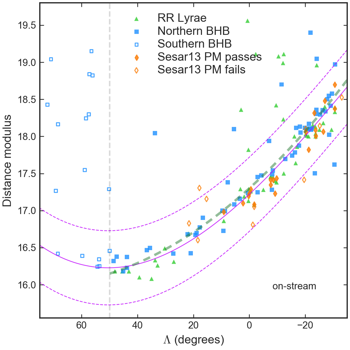
(a)

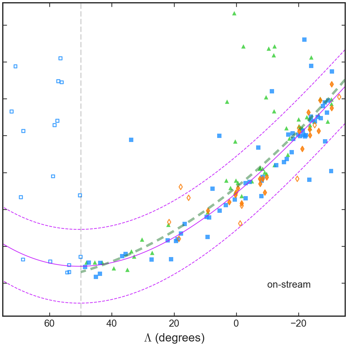
(b)

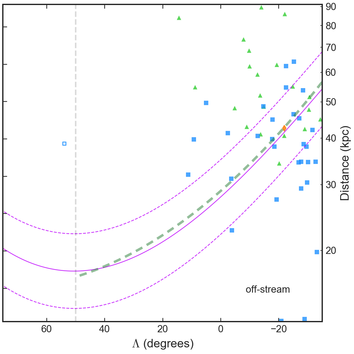
(c)

Figure 1: Panel (a): distance modulus to BHB and RRL stars within the on-stream sky region, defined as a latitude interval $\pm 2.25\degr$ around our adopted spatial track. This panel uses our original distance calibrations, for which RRL stars have systematically lower distances than the BHBs. Proper motion and photometric cuts are applied as discussed in the text. Parallax and data quality cuts are also applied throughout the paper. The boundary of the PS1 survey (vertical line) lies at $\Lambda=50\degr$. RRL stars are taken from the PS1 sample (Sesar et al., 2017) and so are present only in the northern region ($\Lambda<50\degr$). In the southern region ($\Lambda>50\degr$), the BHB selection method uses only  photometry which is less effective at screening contaminants. High-probability stream members from the separate RRL survey of Sesar et al. (2013) are also shown, with point style indicating whether they pass or fail our proper motion cut as indicated by the legend. Stars concentrate around the distance track of Equation 6, shown by the solid line. Short-dashed lines show the limits we use for distance modulus selection. The long-dashed line shows the empirical distance track of Newberg et al. (2010). Panel (b): Same, but using our revised BHB and RRL distance calibrations. The BHB and RRL stars along the stream now agree better on average. Panel (c): Same as (b), but for the off-stream sky region. Here the concentration along the stream track is absent.

BHB stars are excellent distance tracers for metal-poor objects such as the Orphan Stream. While BHB stars are bluer than the main-sequence turnoff and thus less contaminated than redder stars, selection via a single color still mixes in unrelated objects such as blue stragglers, white dwarfs, and quasars. This contamination can be reduced using multiple colors, either in the mid-infrared or using surface-gravity-sensitive colors such as the SDSS $u$-band or the PS1 $z$-band. Vickers et al. (2012) proposed a BHB selection method making use of the $g$, $r$, $i$, and $z$ bands to screen out these contaminants. However, we found these relatively stringent cuts were not well suited to the increased photometric errors as the stream approaches distances of $\sim\!50\,\mbox{kpc}$. To some extent, we can rely on the proper motion to screen contaminants from our stream sample. We will therefore use a more relaxed selection boundary than Vickers et al. (2012), defined as follows:

$$-0.3<g-r<0$$

$$-0.062+0.48\,(g-r)<i-z<-0.02$$

$$-0.30+1.96\,(g-r)<g-z<0+1.96\,(g-r)\;.$$ (1)

In the southern region we have only  photometry which essentially provides a single color. Using old, metal-poor horizontal-branch stars in the MIST isochrone set (Dotter, 2016; Choi et al., 2016) as a guide, we approximate the relationship between $G_{BP}-G_{RP}$ and $g-r$ for these stars as

$$g-r\approx-0.26+0.72\,(G_{BP}-G_{RP})\;,$$ (2)

and then use the $g-r$ cut just stated to obtain a  color cut. Compared to the more elaborate PS1 selection this allows more contaminants, particularly blue stragglers, but we show below that we still can detect the stream in the region of interest.

RR Lyrae stars are also excellent distance tracers, which are in a similar evolutionary stage and have similar luminosities to BHB stars. With a sufficient number of observations, RRL samples can have extremely high purity due to their distinctive light curves. The PS1 RRL sample of Sesar et al. (2017) is a large-scale homogeneous sample where distances are derived from the brightness and time variation in multiple bands. We cross-match this sample to  DR2. We restrict the sample to stars with tabulated RRab score $>0.8$, to avoid mixing in RRc stars and other contaminants.

To guide our analysis, we also use the RR Lyrae radial velocity survey of Sesar et al. (2013) that specifically targeted the Orphan Stream. Candidate RR Lyrae stars in the vicinity of the stream were obtained from several time-series surveys and observed spectroscopically, taking care to correct effects of pulsation phase on the velocity. The sample cross-matched to  DR2 contains 50 total stars spanning the range $-48\degr<\Lambda<22\degr$. Sesar et al. (2013) mark 31 of these as likely stream members based on comparison with distance and velocity tracks from Newberg et al. (2010). The method and data used to compute distance moduli differs between Sesar et al. (2013) and Sesar et al. (2017), but the rms difference is only $0.12$ mag. This level of disagreement is consistent with both samples having independent random distance errors of a mere $\sim\!4\%$.

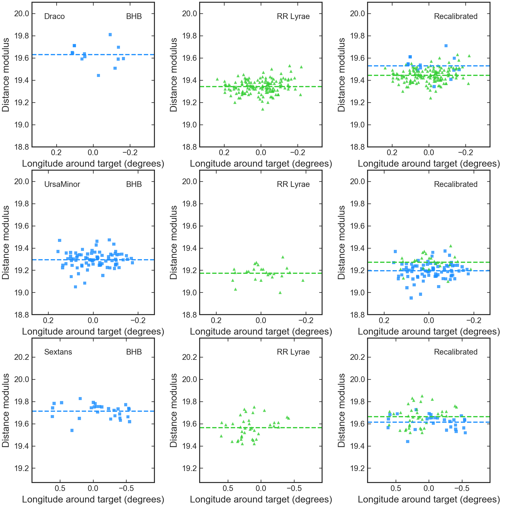
Figure 2: Distance modulus to BHB and RRL stars in dSph galaxies. The rows show results for Draco, Ursa Minor, and Sextans respectively. The horizontal axis shows one sky coordinate and is used merely to separate the points. Each panel uses the same vertical scale. The dashed lines show the median distance modulus for each type. Left column: distance modulus for BHB stars is computed from PS1 photometry with the Deason et al. (2011) calibration. Center column: distance modulus for RRL stars is taken from the table of Sesar et al. (2017). Right column: the same results for both types of star, but using our revised calibration (see Section 2.2).

We initially estimate absolute magnitudes and distance moduli for the BHB stars using the color-based formula of Deason et al. (2011). We make a minor correction from SDSS bands ($g_{S},r_{S}$) to PS1 bands ($g,r$), again using linear relations that approximate colors of horizontal branch stars in the MIST isochrone set:

$$g_{S}-r_{S}=0.014+1.114(g-r)$$

$$M^{\prime}_{\mathit{g_{S},BHB}}(g_{S}-r_{S})=0.434-0.169(g_{S}-r_{S})+2.319(g_{S}-r_{S})^{2}$$

$$\hskip 40.00006pt+20.449(g_{S}-r_{S})^{3}+94.517(g_{S}-r_{S})^{4}$$

$$M^{\prime}_{\mathit{g,BHB}}=M^{\prime}_{\mathit{g_{S},BHB}}(g_{S}-r_{S})-0.014-0.120(g-r)$$ (3)

Here the prime on the mean BHB absolute magnitude $M^{\prime}_{\mathit{g,BHB}}$ indicates it is an initial calibration that we will adjust later. For the southern region where only  photometry is available, we use approximate transformations between  and SDSS bands (again based on MIST isochrones) to apply the relation above:

$$g_{S}-r_{S}=-0.27+0.80(G_{BP}-G_{RP})$$

$$g_{S}-G=-0.15+0.60(G_{BP}-G_{RP})$$

$$M^{\prime}_{\mathit{G,BHB}}=M^{\prime}_{\mathit{g_{S},BHB}}(g_{S}-r_{S})-(g_{S}-G)$$ (4)

We use an initial guess for the stream latitude that closely follows the results of Newberg et al. (2010) and Grillmair et al. (2015). Our spatial selection uses stars within $2.25\degr$ of this track. Assuming the $0.9\degr$ latitude dispersion estimated by Belokurov et al. (2006), this is approximately $2.5\sigma$. We also initially require the estimated distance modulus to lie within 0.5 mag of the track of Newberg et al. (2010). Binning the stars in $10\degr$ intervals of $\Lambda$, we find a clump of stars lying at high $\mu_{\Lambda}$ for $\Lambda\sim 50\degr$. This clump can be followed over the entire range of $\Lambda$ in the northern sample, though it is less distinct from the background population at low $\Lambda$. Fitting the values found from the bins, we obtain an initial smooth track for the stream’s proper motion. When the distance moduli of stars near this proper motion track are plotted versus $\Lambda$, a distinct stream is apparent. Figure 1 shows the BHB stars as cyan points in the left panel, with solid symbols denoting the northern sample using PS1 photometry and open symbols the southern sample. In the figure we use our final stream proper motion and position tracks to define the sample, in order to present only our final converged results. A similar concentration is not seen in the sample of stars outside our latitude cut.

We then apply the same position and proper motion cuts to the RR Lyrae sample, in which a clump can be found in proper motion space following the same trend as the BHB stars. Using the default distance modulus values from Sesar et al. (2017), this yields a similar concentration along the stream distance track (green points in left panel of Figure 1). Thus we have a clear detection of the Orphan Stream in the  data.

In panel (a) of Figure 1 there appears to be an offset between the BHB and RR Lyrae stars, with the latter apparently nearer on average. (A similar offset is suggested by figure 1 of Sesar et al., 2013, with the majority of the stream RR Lyrae on the near side of the orbital tracks from Newberg et al., 2010.) It seems unlikely that these two types of stars could consistently lie at different distances over such a long stretch of the stream, whereas a mismatch of our distance scales would not be particularly surprising. There are several places where systematic error could arise, including our translation from the SDSS-based distance scale to PS1 and  for the BHB stars. Both the Deason et al. (2011) BHB and Sesar et al. (2017) RR Lyrae magnitudes are calibrated against globular clusters. It is likely that both calibrations should be affected by metallicity, but neither sample takes this into account explicitly. Furthermore, the relationship between BHB and RRL stars might be different in globular clusters vs dwarf galaxies, and Orphan appears to be a remnant of the latter class. In dwarf galaxies one might expect that whether a star winds up as a BHB or an RRL is primarily due to metallicity. A globular, in contrast, typically has a very small metallicity ($[\mathrm{Fe}/\mathrm{H}]$) range, but also has sub-populations with inferred differences in helium abundances and relative metal abundance patterns. These differences, rather than just the value of $[\mathrm{Fe}/\mathrm{H}]$, are likely to determine whether a star winds up as a BHB or an RRL. It thus seems plausible that the BHB and RRL distance scales are not completely consistent for the stream sample here.

We therefore recalibrate the BHB and RRL distances using three dSph galaxies with metallicities similar to that of the Orphan Stream: Draco, Ursa Minor, and Sextans. With our original calibrations, we find in each case an offset between BHB and RRL stars in the same direction as for the Orphan Stream (Figure 2), although its size seems to vary a bit. The mean offset in these three galaxies is 0.19 mag. To reconcile the distance scales, we simply split the difference. We add 0.1 mag to the absolute magnitude formula of Deason et al. (2011): implying a distance modulus 0.1 mag smaller.

$$M_{\mathit{g,BHB}}=M^{\prime}_{\mathit{g,BHB}}+0.10$$

$$M_{\mathit{G,BHB}}=M^{\prime}_{\mathit{G,BHB}}+0.10$$ (5)

We also subtract 0.1 mag from the PS1 RRL absolute magnitudes, or equivalently assume a distance modulus 0.1 mag larger than given in the original table. The recalibrated distance moduli for the Orphan sample are shown in the panel (b) of Figure 1. Panel (c) of Figure 1 shows the BHB and RRL in the off-stream region. The strong concentration along the stream distance track is absent in this plot, confirming that it originates from the Orphan Stream.

Of course, given that the distance scales for both types of object are uncertain, our newly reconciled distance scale is also uncertain. For an additional test we matched the RRL passing all of our sample cuts to the sample of Hendel et al. (2018). This sample uses near-infrared photometry of the stars in Sesar et al. (2013) and thus arguably has better distance estimates than Sesar et al. (2017), though sources of systematic error remain. We find the median difference in distance modulus between our recalibrated values and those of Hendel et al. (2018) is $0.04$ mag, or a distance offset of only 2%. This is probably within the level of systematic error for the stellar tracers used here, and we regard it as acceptable agreement.

The distance modulus of the stream appears well described by the curve

$$\mathit{DM}(\Lambda)=17.22-3.52\,\Lambda_{100}+2.29\,\Lambda_{100}^{2}+1.58\,\Lambda_{100}^{3}$$

$$\Lambda_{100}\equiv\Lambda/100\degr$$ (6)

The track is in reasonable agreement with the empirical track of Newberg et al. (2010) shown with the long-dashed line, but puts the stream slightly closer for much of the observed range. Furthermore, our track flattens at $\Lambda=50\degr$ above which the distance rises again, though the exact form of this turn-up is uncertain due to the small number of stars constraining it.

The dispersion in magnitude around this track appears to be roughly 0.2 mag for RRL stars, and 0.3 mag for BHB stars. This implies an upper limit on the overall distance dispersion of $\approx 10$–15%. These dispersions most likely stem from the combined effects of sample contamination and intrinsic dispersion in the source brightnesses, rather than the intrinsic thickness of the stream. Using near-infrared photometry, Hendel et al. (2018) formally estimated a distance dispersion of 0.22 mag around their orbital track. We note that in that paper as well as this one, much of the overall dispersion appears to originate at the northern end of the stream, whereas the portion in $0\degr<\Lambda<50\degr$ is much better collimated.

Figure 1 also shows for comparison the 28 high-confidence stream RRL from Sesar et al. (2013) that fall within our latitude cut, with closed (open) symbols denoting those that pass (fail) our proper motion cut. Although most of these 28 stars pass our cut, 10 do not. The 7 stars labeled RR19, RR30, RR31, RR43, RR46, RR47, RR49 are offset from our trend by more than $1\,\mbox{mas}\,\mbox{yr}^{-1}$ in either longitude or latitude directions, compared to typical errors of $0.3\,\mbox{mas}\,\mbox{yr}^{-1}$. Hendel et al. (2018) previously noted the tension between  measurements and expectations for five of these stars, and furthermore found that another (RR19) has a light curve inconsistent with a genuine RRL star. The stars failing the proper motion cut are outliers in several other ways. They include the four at highest $\Lambda$, in the Galactic longitude range $245\degr<l<258\degr$ in figure 2 in Sesar et al. (2013). They also include the four “stream” stars most discrepant from our distance tracks. Finally, they also include the two stars with the highest metallicity in the “stream” sample (RR46 and RR47). Sesar et al. (2013) noted both a significant metallicity dispersion and significant gradient of spectroscopic metallicity along the stream. Removal of these stars would significantly suppress both of these properties. It would however not eliminate either entirely, which is significant insofar as it relates to the nature of the stream’s progenitor.

2.3 Velocity and stellar population from spectroscopic sample

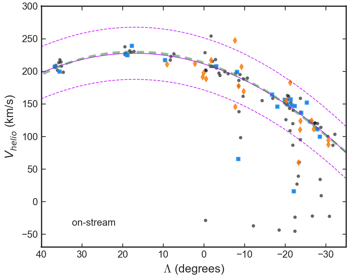
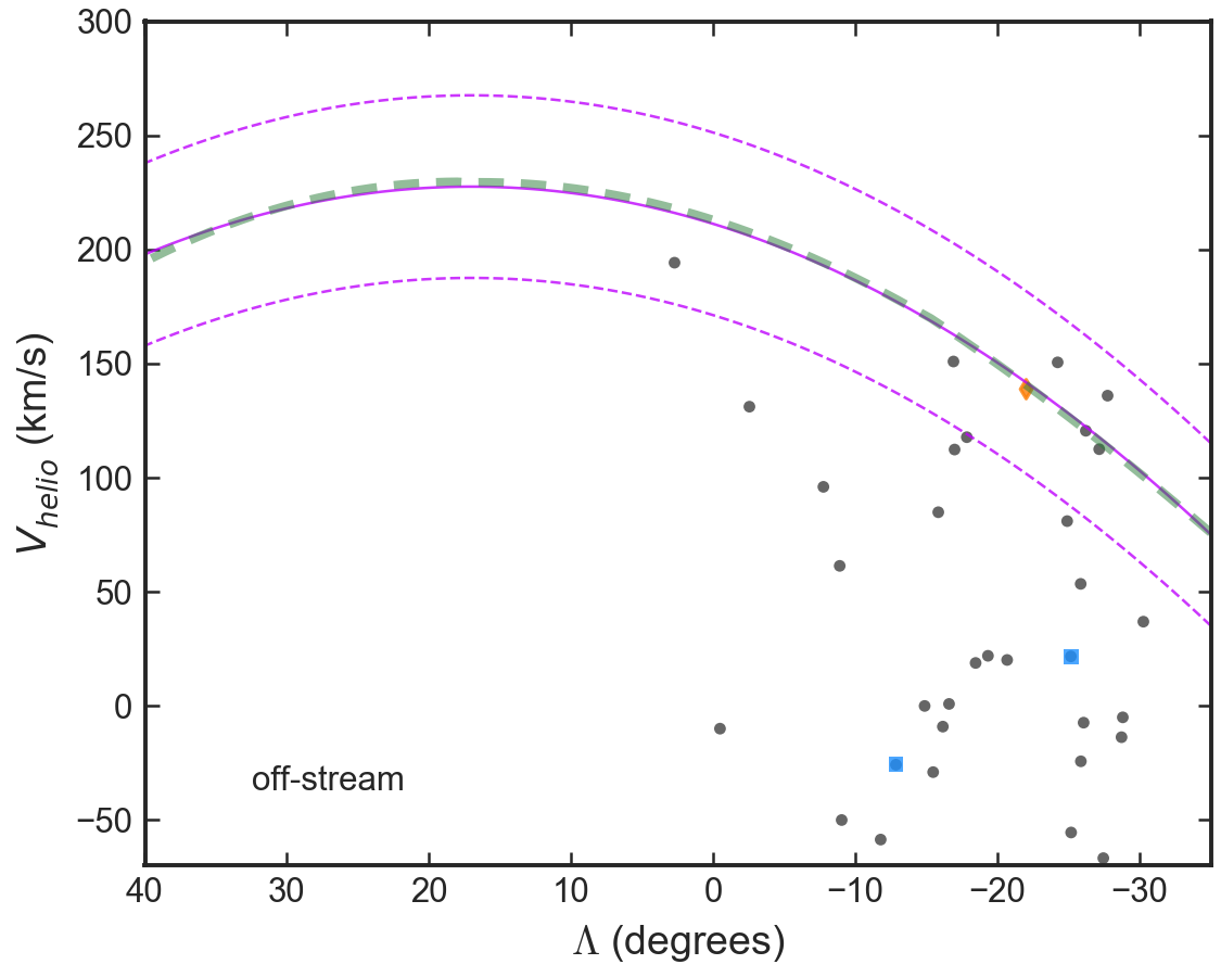
Figure 3: Left: velocity of stars from SDSS in the on-stream latitude region. Black circles are selected according to the standard spatial and proper motion cuts. Cyan squares show stars additionally passing photometric and distance modulus selection cuts for BHB stars. The solid line shows our fit to these points (equation 7). Dashed lines show our selection boundary of $\pm 40\,\mbox{km}\,\mbox{s}^{-1}$ around this track. The dashed green line shows the nearly identical track of Newberg et al. (2010). Orange diamonds show high-confidence RRL from Sesar et al. (2013), with an additional cut on proper motion made as for the other stars. Right: same, but for the off-stream latitude region.

At this stage, we have useful approximations of the distance and proper motion trends in the sample. We would like to select RGB stars as well, to constrain the stellar population and refine the proper motion trends. First, though, we need to know their location in the color-magnitude diagram (CMD). RGB stars lie in a more contaminated region of the CMD than the BHB stars. To obtain the cleanest possible sample, we would like to combine parallax and proper motion cuts using  data with selection on radial velocity.

For this purpose, we obtain spectroscopic stars from the SDSS DR13 archive within the sky area of interest and cross-match this sample to our previous  DR2 and PS1 sample. The SDSS sample includes widely distributed stars from the “legacy” survey, and spots sampled at a higher density due to the SEGUE programs. The DR13 sample is somewhat larger than that available to Newberg et al. (2010). We continue to use PS1 as our source of photometry to enable a homogenous selection over the largest possible sky area. We use the fields elodiervfinal, fehadop, and loggadop for the radial velocity, $[\mathrm{Fe}/\mathrm{H}]$, and $\log\,g$ parameters respectively.

In Figure 3 we show the velocity trend obtained using our standard latitude, parallax, and proper motion cuts. The stream is easily picked out by eye, especially when comparing with the off-stream sample. Truncating outliers, we fit the data with the curve

$$v_{\mathit{helio}}(\Lambda)=(211+192\,\Lambda_{100}-563\,\Lambda_{100}^{2})\,\mbox{km}\,\mbox{s}^{-1}$$ (7)

We also show the track of Newberg et al. (2010), translated from their galactic standard of rest frame back to heliocentric velocity. Despite our advantages of a cleaner and slightly larger sample, the earlier track is almost identical. Due to the coverage limits of SDSS, this track has only been tested over $-35\degr\la\Lambda\la 40\degr$, a smaller longitude range than for the tracks in the other data dimensions.

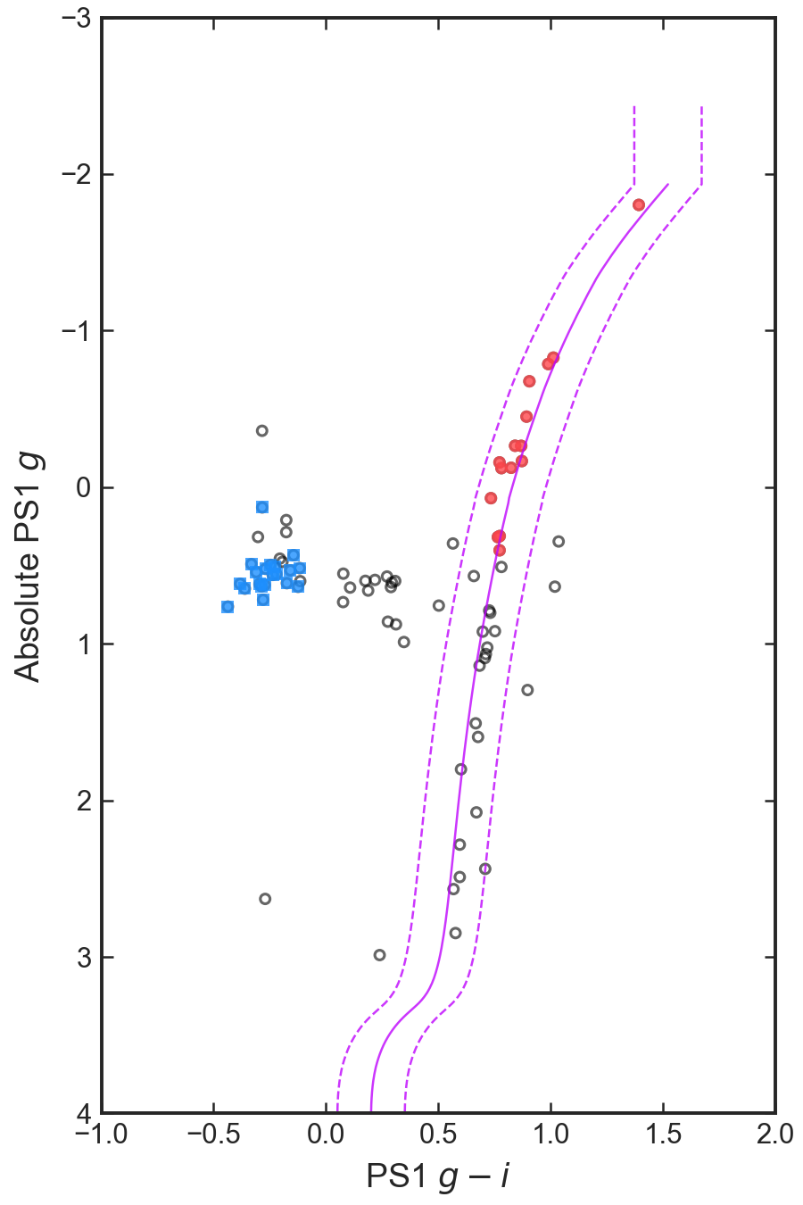
(a)

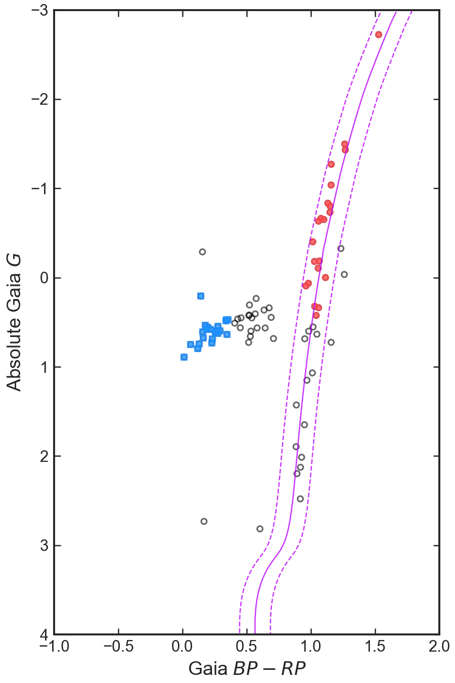
(b)

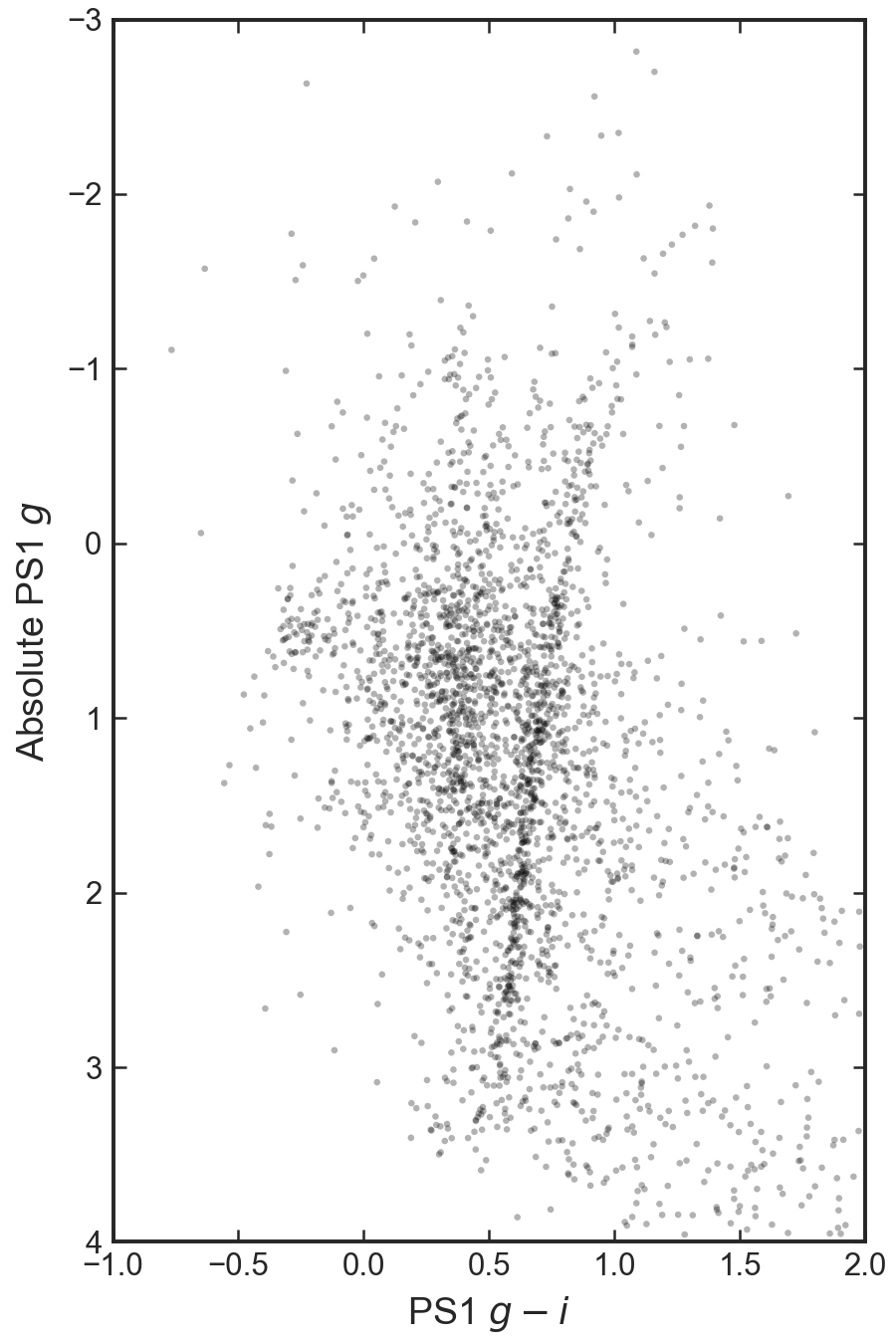
(c)

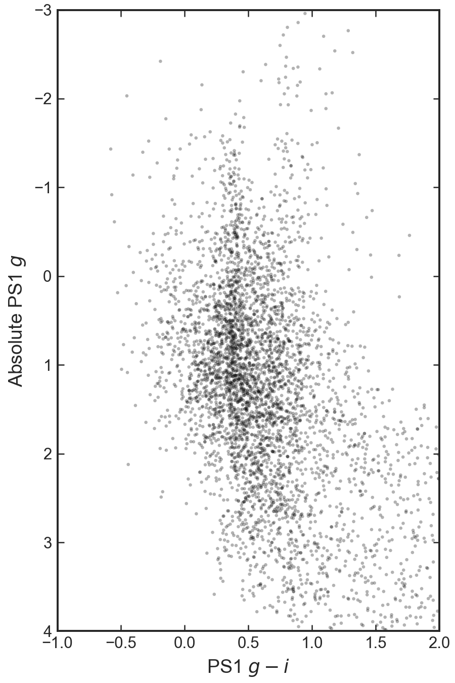
(d)

Figure 4: Panel (a): color - absolute magnitude diagram for the spectroscopically selected sample, from PS1 photometry. Absolute $g$ magnitude and $g-i$ color are corrected for extinction and computed according to the distance modulus fit in Equation 6. Points show all stars passing latitude, proper motion, and velocity cuts. Red points show stars passing the RGB selection cut based on PS1 photometry. Cyan points show BHB candidates. The solid line shows a $[\mathrm{Fe}/\mathrm{H}]=-1.75$, $13\,\mbox{Gyr}$ MIST isochrone. Dashed lines show the RGB selection boundaries around this isochrone (we also impose a brightness limit $M_{g}<0.5$). Panel (b): Same, but using  photometry and stellar type selection criteria. The central isochrone in this case is $[\mathrm{Fe}/\mathrm{H}]=-1.5$, $13\,\mbox{Gyr}$. Panel (c): stars in the on-stream sky region drawn from the overall  DR2 $+$ PS1 sample in the northern region. Cuts are applied in proper motion, parallax, and data quality. The Orphan Stream is visible as the extremely narrow curving RGB sequence and the cloud of HB stars. Panel (d): same, but for the off-stream sky region. The signatures of the Orphan Stream seen in Panel (c) are absent.

To our previous selection cuts, we now add a cut of $\pm 40\,\mbox{km}\,\mbox{s}^{-1}$ around the velocity track. The stars selected in this manner are plotted in the color - absolute magnitude diagram in Figure 4a. This shows a well-developed RGB, a strong concentration of BHB and possible RRL stars, and even a hint of the asymptotic giant branch where it joins onto the RGB. As noted by Newberg et al. (2010), the selection of stars in SDSS is complicated and far from uniform, so the relative numbers of stars in different parts of the CMD (e.g., BHB vs RGB) are not fair reflections of the underlying population. However, the appearance of a narrow RGB is unlikely to be an artifact.

Using $3\sigma$ clipping, we estimate the velocity dispersion about the mean track as $\sigma_{v}=7\,\mbox{km}\,\mbox{s}^{-1}$. This is close to the estimate $8$–$13\,\mbox{km}\,\mbox{s}^{-1}$ of Newberg et al. (2010). Hendel et al. (2018) estimated a much larger velocity dispersion of $30\,\mbox{km}\,\mbox{s}^{-1}$ about their orbital tracks. As they note, however, it is difficult to measure velocities of RRL due to their atmospheric motion, and the much smaller dispersions found here are probably more reliable.

We find a MIST isochrone of $[\mathrm{Fe}/\mathrm{H}]=-1.75$ and age $13\,\mbox{Gyr}$ fits the stars reasonably well. (We use the MIST v1.1 isochrones with $v_{\mathit{crit}}=0$ and solar $[\alpha/\mbox{Fe}]$ throughout.) From this we construct a selection boundary in the CMD (Figure 4a) with width 0.2 mag on either side of the isochrone. We also impose an absolute magnitude limit $g<0.5$, as this keeps the dwarf contamination low and uses only the stars with the most accurate proper motions. Using the stars within this CMD cut, the mean spectroscopic metallicity is found to be $[\mathrm{Fe}/\mathrm{H}]=-2.0$ with dispersion $\sigma_{[\mathrm{Fe}/\mathrm{H}]}=0.4$. This dispersion is almost entirely real, assuming the formal uncertainties are valid, as the dispersion induced by observational error is $<0.2$ dex. Given the many assumptions that go into specifying the isochrone and the possibilities for observational error, the offset between our photometry and spectroscopic metallicity estimates is not particularly surprising.

In Figure 4b we show a similar diagram but using  photometry. A distinct RGB remains, though it is slightly less tight than in Figure 4a. Here we find a better isochrone has $[\mathrm{Fe}/\mathrm{H}]=-1.5$ with age $13\,\mbox{Gyr}$. We use a selection boundary with half-width 0.15 mag to choose stream stars. Again, we will not be troubled by the slight disagreement with the spectroscopic metallicity.

The stellar population of the stream is also vividly illustrated using the overall  PS1 sample without any spectroscopic selection, with much higher signal though also higher contamination. The stream signature is obvious in the on-stream region in Figure 4c, whereas it is absent in the off-stream region in Figure 4d. Although we have omitted the isochrone to improve the plot clarity, it agrees with the narrow RGB down to faint magnitudes, well below our absolute magnitude cut. The RGB is slightly wider but still easily visible when using  photometry alone.

Casey et al. (2013) obtained spectra of stream candidates in a field spanning the longitude range $15$–$25\degr$, and identified 9 stars as stream members. It turns out that while 5 of them are in the proper motion range we identified as belonging to the stream, 4 of them are not. Of the 4 non-members (OSS 4, 9, 12, and 19), 3 have higher metallicities than the rest of the sample. As with the Sesar et al. (2013) sample, pruning the sample with proper motion reduces the mean metallicity and dispersion in this sample, but does not eliminate the dispersion. The revised mean metallicity from the 5 remaining stars would be $-2.1$, with dispersion 0.5. Casey et al. (2014) obtained high-resolution spectra and improved metallicity estimates of 3 of the Casey et al. (2013) stream candidates (OSS 6, 8, and 14). All three of these pass our proper motion cut and are thus highly likely to be stream members. These stars span a range of over 1 dex in $[\mathrm{Fe}/\mathrm{H}]$, supporting a substantial metallicity dispersion within the stream and disfavoring a globular cluster as the progenitor.

2.4 Proper motion

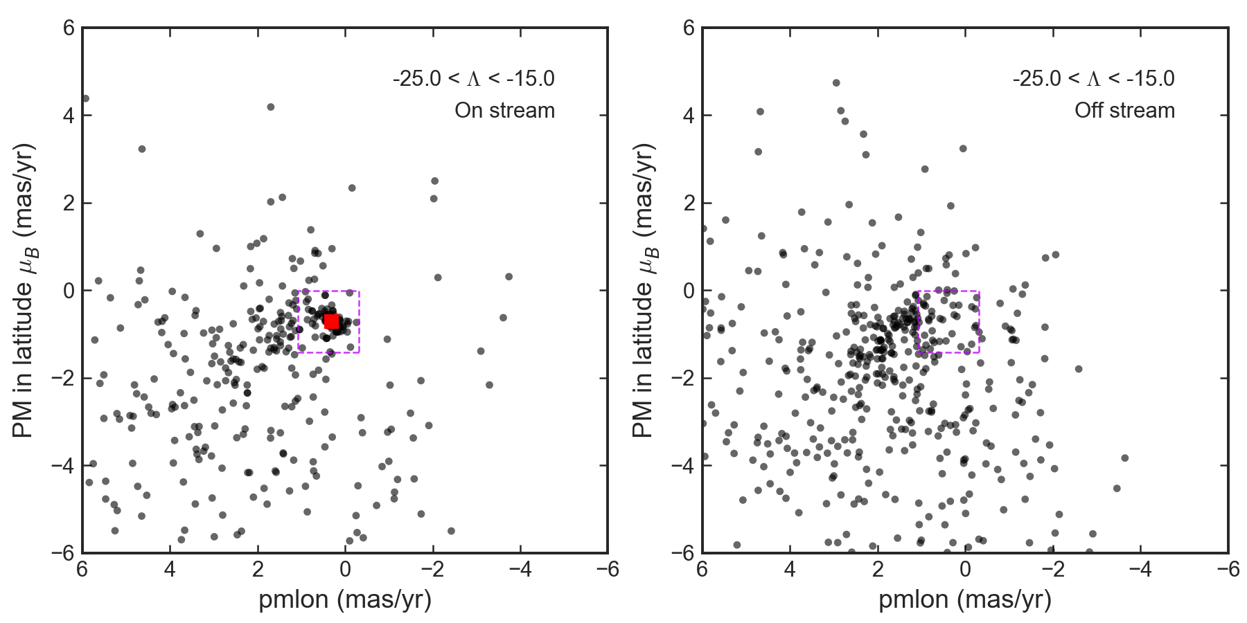
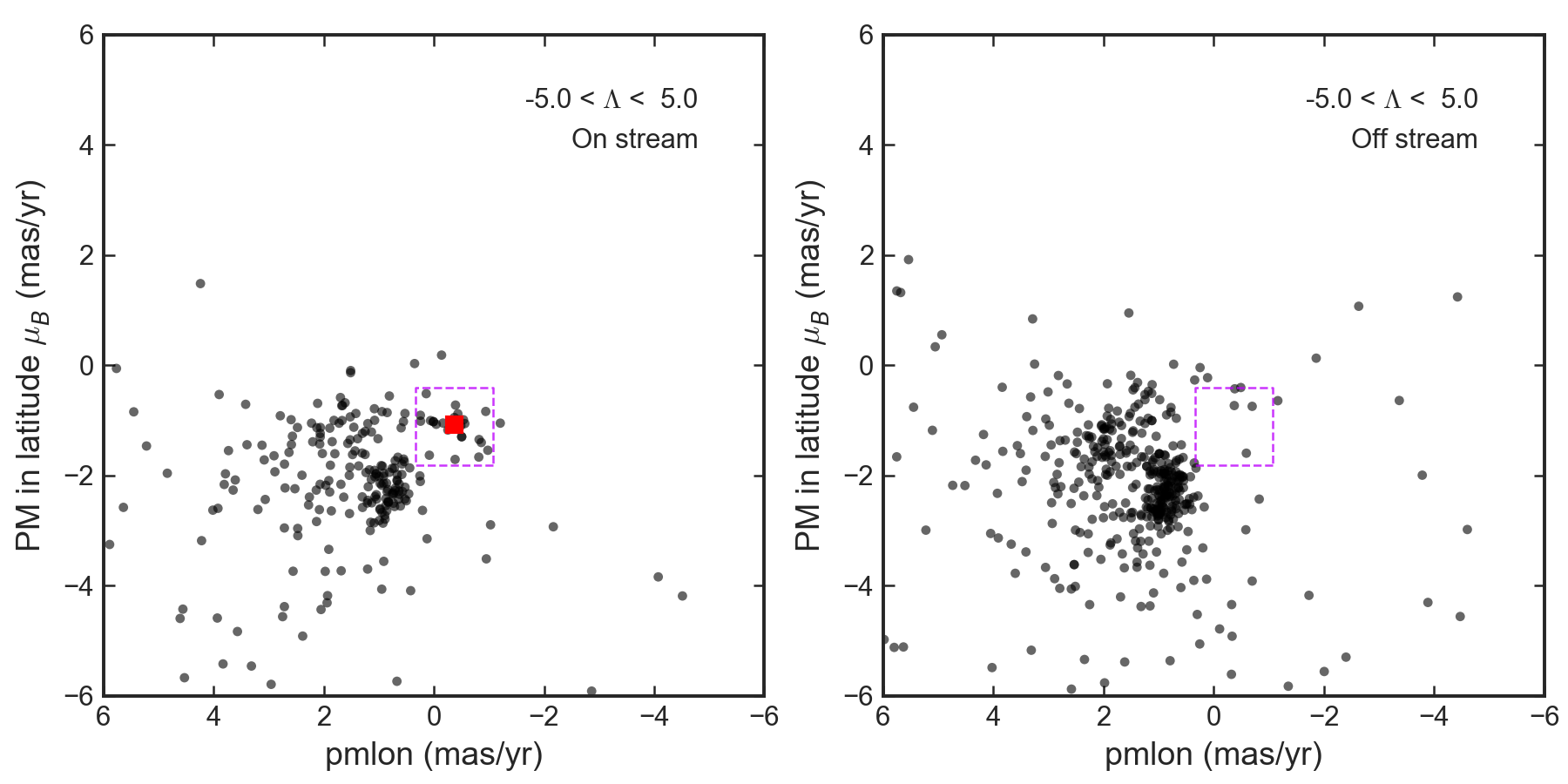
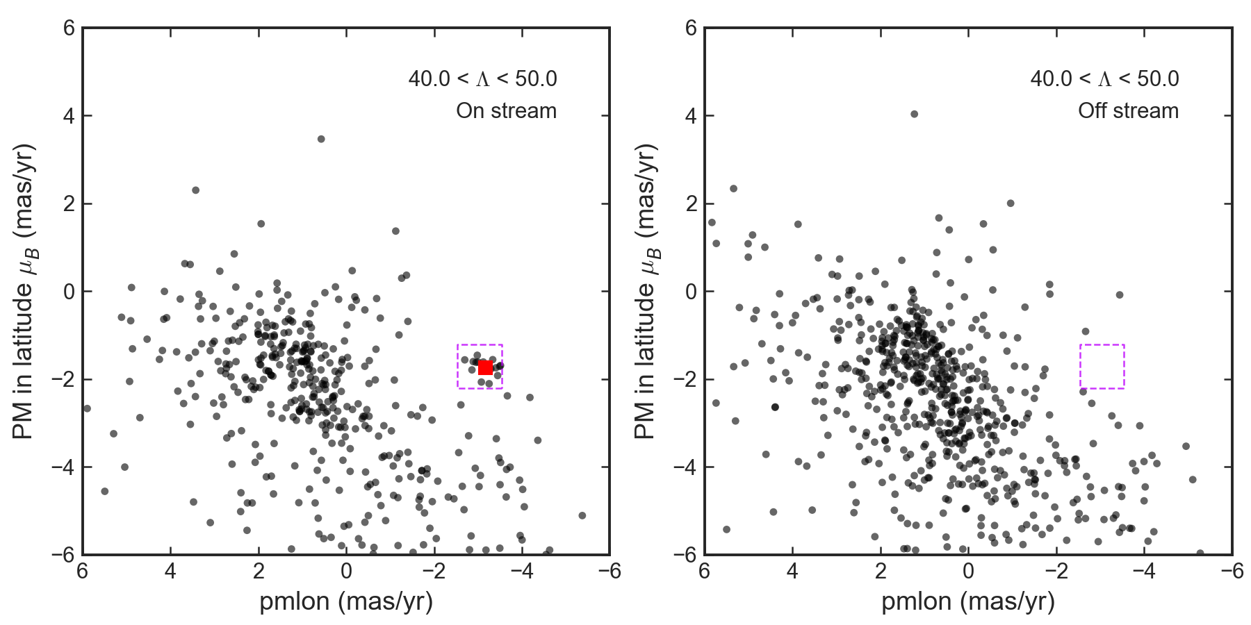
Figure 5: Proper motion of stars in the Orphan Stream region. Each row shows a different bin of $10\degr$ in longitude $\Lambda$. Left column: on-stream region defined by a latitude interval centered on the stream track. Right column: off-stream region, where the stream concentration is absent. Black points show sample stars, including RGB, RRL, and BHB stars, selected based on photometry as appropriate to stellar type. The red point shows the fit to the mean stream proper motion in this bin. The dashed box shows the square PM selection box, which is centered on the smooth track of Equation 8. The dense clump near $(-1\,\mbox{mas}\,\mbox{yr}^{-1},-2\,\mbox{mas}\,\mbox{yr}^{-1})$ in both panels of the second row is from the Sagittarius Stream (see text).

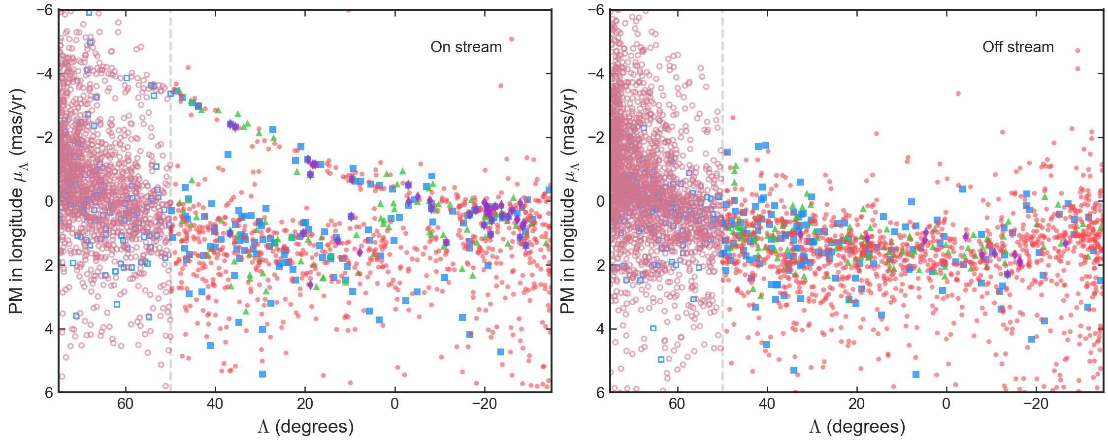
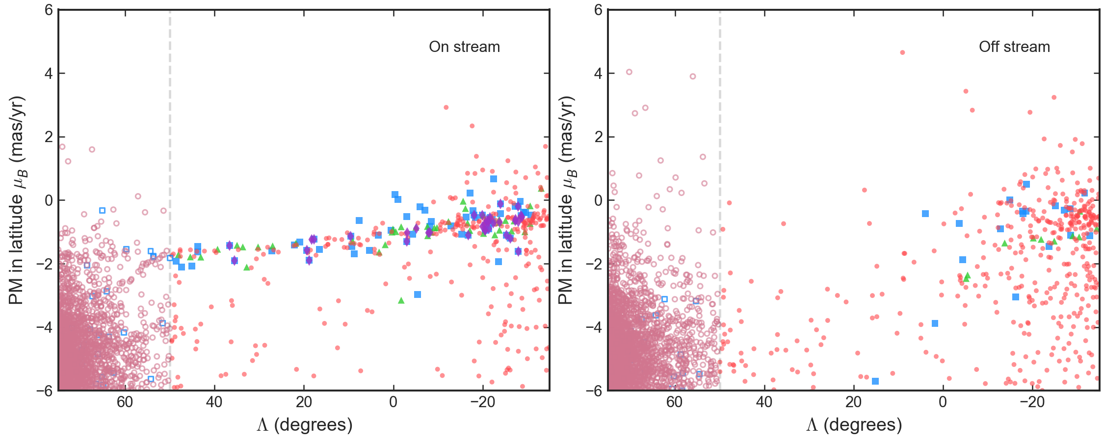
Figure 6: Proper motions of stars along the Orphan Stream path. Top and bottom rows show proper motions in longitude and latitude $(\mu_{\Lambda},\mu_{B})$. Left column: on-stream sky region selected by a latitude cut around the stream track. Right column: off-stream sky region. Data points show individual stars coded according to selection method. Solid cyan squares: northern BHB; empty cyan squares: southern BHB; green triangles: RRL; solid red circles: northern RGB; empty pink circles: southern RGB; purple diamonds: velocity-selected spectroscopic sample. For each dimension, cuts are applied to the stars in all other observable dimensions—i.e. for the $\mu_{\Lambda}$ plots, stars are selected based on $\mu_{B}$, and vice versa. All panels also use selection on spatial position (on or off stream), and distance modulus or CMD cuts as appropriate to the stellar type. The Orphan Stream is visible as the narrow band following the high-purity spectroscopic points.

We already used an initial proper motion cut based on the BHB and RRL subsamples to help select stream stars and define the behavior in other dimensions. Now we add the information from RGB stars, some of which are quite bright and therefore have small proper motion uncertainties, to define the proper motion trend more precisely.

We divide our entire sky region into longitude bins $10\degr$ long, overlapping by $5\degr$ so that only every second bin is independent. We combine our BHB, RRL, and RGB samples selected by parallax and by distance modulus (for BHB and RRL) or color-magnitude position (for RGB) as described above. We switch between the northern and southern selection methods at $\Lambda=50\degr$. In each bin, we select stars inside and outside our latitude cut of $\pm 2.25\degr$ around the stream track for the signal and background samples respectively. We use only stars within the box $|\mu_{\Lambda}|<6\,\mbox{mas}\,\mbox{yr}^{-1}$, $|\mu_{B}|<6\,\mbox{mas}\,\mbox{yr}^{-1}$. This separates our estimation of the stream proper motion from details of the distribution at much higher proper motions, which correspond to nearby disk stars.

The combined sample in several bins is shown in Figure 5. In each bin, a clump of stars associated with the stream is apparent, though in some bins it is stronger or more distinct than in others. Over a latitude range $-20\degr<\Lambda<10\degr$, a strong second cold clump is apparent in both the on-stream and off-stream samples. From its sky position (RA $\approx 153\degr$, declination $\approx 23\degr$) and proper motion, this clump is identifiable as the leading arm of the Sagittarius Stream.

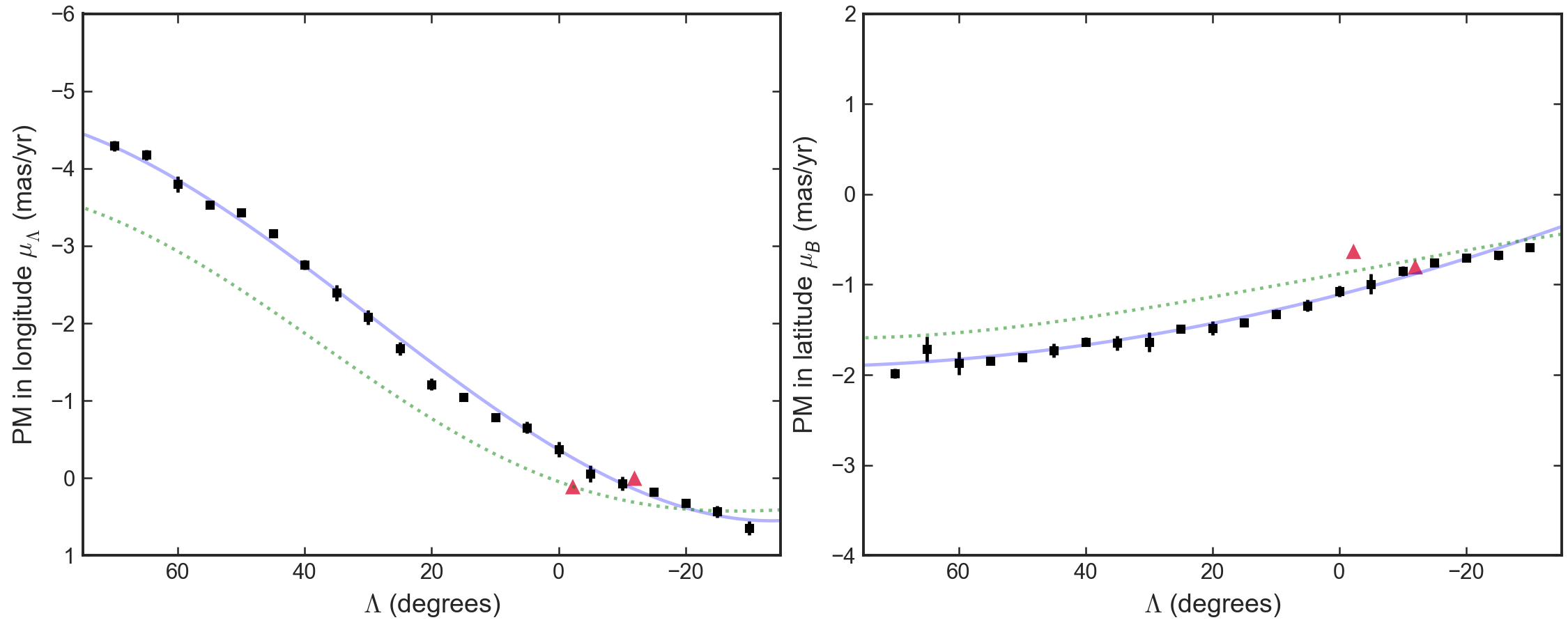
Figure 7: Proper motion tracks of the Orphan Stream in longitude (left) and latitude (right) directions. The data points show results from fits to $10\degr$ bins. The bins overlap by $5\degr$ so only every second bin is independent. The solid line shows our fit to these points (equation 8). Red triangles show the detections of Sohn et al. (2016). The dotted line shows orbit 5 from Newberg et al. (2010).

We first use the Gaussian Mixture Model code pyggmis to fit the background (off-stream) sample of each bin in the space of $(\mu_{\Lambda},\mu_{B})$, using a Gaussian mixture of either 2 or 3 components depending on the apparent complexity of the off-stream sample in that bin. We choose this particular code because it corrects for the censored data outside our proper motion box. We then add another component to represent the stream in the signal region, and initialize the guess for this component’s center to the value given by our previously derived trend. We initialize the other components to the values given by the background fit. We run pyggmis on the signal region data to obtain a fit to the stream proper motion. We then bootstrap-resample the points and repeat the procedure to obtain estimates of the uncertainties. The final fitted values are shown by the points in Figure 5 centered on the stream clump.

Once we have a fit to the mean stream proper motion within each longitude bin, we fit the overall trend with a cubic in $\Lambda$ for $\mu_{\Lambda}$ and a quadratic for $\mu_{B}$, yielding the tracks

$$\mu_{\Lambda}=(-0.31-4.73\,\Lambda_{100}-6.04\,\Lambda_{100}^{2}+6.86\,\Lambda_{100}^{3})\,\mbox{mas}\,\mbox{yr}^{-1}$$

$$\mu_{B}=(-1.10-1.85\,\Lambda_{100}+1.03\Lambda_{100}^{2})\,\mbox{mas}\,\mbox{yr}^{-1}$$ (8)

The trends of the on and off-stream samples with latitude are shown with individual stars in Figure 6. Here we use Equation 8 to select stars in the proper motion dimension that is not plotted, along with our other usual sample cuts. (Without this additional cut, the contrast of the stream versus the background would be greatly reduced.) Left panels show the on-stream sky region, and right panels the off-stream region. It is easy to pick out the stream in the on-stream regions, while it is essentially absent from the off-stream region. Some interesting hints of substructure are present through the increased dispersion at certain locations and the possible kink in $\mu_{B}$ near $\Lambda=50\degr$. We will not pursue these further here.

The individual bin fits and the track given by Equation 8 are displayed in Figure 7. The PM estimates of Sohn et al. (2016) are shown by the two red triangles. These estimates were obtained by finding stars roughly matching the main sequence at the distance of the stream as well as the proper motion of the stream as predicted by Newberg et al. (2010). Converting the Sohn et al. (2016) values to stream coordinates, the field at $\Lambda=-12.0\degr$ has $\mu_{\Lambda}=0.0\,\mbox{mas}\,\mbox{yr}^{-1}$, $\mu_{B}=-0.80\,\mbox{mas}\,\mbox{yr}^{-1}$, and the field at $\Lambda=-2.2\degr$ has $\mu_{\Lambda}=0.11\,\mbox{mas}\,\mbox{yr}^{-1}$, $\mu_{B}=-0.63\,\mbox{mas}\,\mbox{yr}^{-1}$. The point at $\Lambda=-12\degr$ is in excellent agreement with our results. The point at $\Lambda=-2\degr$ deviates somewhat in both dimensions, which is not surprising—this point represents the lone star in that field consistent with expected stream properties.

Figure 7 include the prediction of orbit 5 from Newberg et al. (2010) (their best fit), which we recomputed with the aid of the galpy package. This orbit agrees reasonably well with our fit around $\Lambda=-20\degr$. Its slope and curvature also agrees qualitatively with our results in both dimensions. Quantitatively, however, this orbit is ruled out by our results at very high significance, and the absolute differences reach as high as $\ga 1\,\mbox{mas}\,\mbox{yr}^{-1}$.

To define sample cuts based on proper motion, we center our selection box on the fit given by Equation 8. In the northern region we use a box of a fixed half-width $0.7\,\mbox{mas}\,\mbox{yr}^{-1}$ in each proper motion dimension $(\mu_{\Lambda},\mu_{B})$ separately, centered on the trend of Equation 8. In the southern region the proper motion errors are smaller and the contamination of the RGB and BHB samples is greater, so we decrease the box half-width to $0.5\,\mbox{mas}\,\mbox{yr}^{-1}$.

Since stream coordinates for the proper motion may not be preferable in all cases, we re-express the proper motion trends in Equation 8 in equatorial coordinates with the approximate fits

$$\mu_{\mathit{RA}}=(-1.17-3.33\,\Lambda_{100}-0.13\,\Lambda_{100}^{2}-0.22\,\Lambda_{100}^{3})\,\mbox{mas}\,\mbox{yr}^{-1}$$

$$\mu_{\mathit{Dec}}=(-0.06+4.21\,\Lambda_{100}+4.89\,\Lambda_{100}^{2}-6.88\,\Lambda_{100}^{3})\,\mbox{mas}\,\mbox{yr}^{-1}$$ (9)

In galactic coordinates we find

$$\mu_{\mathit{l}}=(-0.42-7.35\,\Lambda_{100}-4.63\,\Lambda_{100}^{2}+19.72\,\Lambda_{100}^{3}$$

$$\hskip 40.00006pt-12.58\,\Lambda_{100}^{4})\,\mbox{mas}\,\mbox{yr}^{-1}$$

$$\mu_{\mathit{b}}=(-1.04-0.27\,\Lambda_{100}+11.64\,\Lambda_{100}^{2}+2.12\,\Lambda_{100}^{3}$$

$$\hskip 40.00006pt-12.37\,\Lambda_{100}^{4})\,\mbox{mas}\,\mbox{yr}^{-1}$$ (10)

The accuracy of these fits should be better than $0.1\,\mbox{mas}\,\mbox{yr}^{-1}$, except possibly near the ends of the observed range $-35\degr<\Lambda<75\degr$.

2.5 Sky position

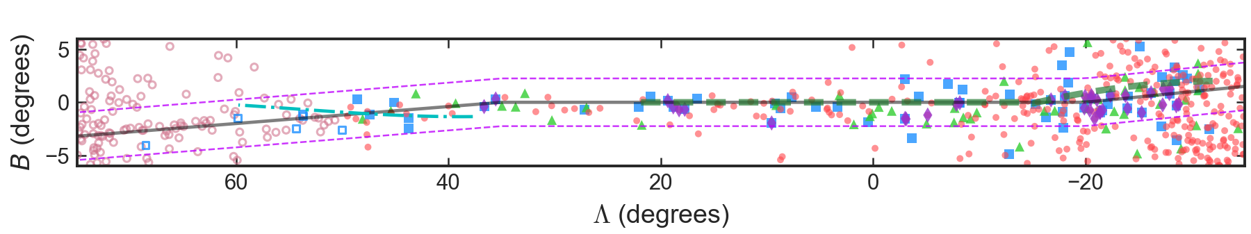
Figure 8: Spatial distribution of sample sources. Point types correspond to stellar type as in Figure 6. Stars are selected according to photometry, proper motion, and (for the spectroscopic sample) velocity. The stream is quite clean and concentrated in $0\degr\la\Lambda\la 50\degr$ or so, while the contamination increases at both low and high $\Lambda$. Nevertheless a concentration is clearly visible in the north (low $\Lambda$) roughly following the bend in the track found by Newberg et al. (2010) (green dashed line). Cyan line shows the track of Grillmair et al. (2015). In the south (high $\Lambda$), the stream appears to veer towards negative $B$ at least up to $\Lambda=65\degr$ and perhaps further. Solid black line shows our adopted stream track. Dashed magenta lines show our on-stream latitude selection cut, $2.25\degr$ on either side of this track.

To refine the track of the stream on the sky, we now select stars according to the parallax, proper motion, and distance modulus or color-magnitude properties of the stream. Figure 8 shows the stars from our various samples plotted on the sky in stream coordinates. Here increasing contamination is apparent in the north (low $\Lambda$) because the proper motion cut loses discriminating power there, due to the smaller separation from the background stars. Still, it appears the stream roughly follows the bend to larger latitude $B$ at low $\Lambda$ already found by Newberg et al. (2010).

In the south (large $\Lambda$), the increasing contamination again makes the stream difficult to follow. Nevertheless, we find the stream stars have their peak density at lower and lower $B$ as $\Lambda$ increases, reaching a deviation of at least $2\degr$ from the equator of the coordinate system. The Orphan Stream in the south was previously mapped by Grillmair et al. (2015) using stars near the main-sequence turnoff. They found a change from a fairly well-defined stream over $-38\degr<\delta<-18\degr$ ($38\degr<\Lambda<60\degr$) to a broader and bifurcated structure further south. They attributed the brightest structures in the southern section to inaccurate correction of the highly structured extinction in this area. Our stream map consists of stars from entirely different parts of the color-magnitude diagram than in Grillmair et al. (2015), yet we find an overdensity in the same regions as the brightest overdensities in their maps. This suggests these overdensities may be real. Our stream path does not closely follow the analytic fit provided by Grillmair et al. (2015) or show the S-shaped bend at $\delta=-14\degr$ ($\Lambda=34\degr$), but the density of our tracers is particularly low in this area so it is not clear if there is a real disagreement.

Given the hints of irregular spatial structure and the relatively small signal, we have not performed a fully automatic fit to the stream track. Instead, we matched a piecewise linear trend, modifying the earlier trend of Newberg et al. (2010), to follow the apparent stream overdensity in Figure 8:

$$B=-0.10\,(\Lambda+20\degr),\;-35\degr<\Lambda<-20\degr$$

$$B=0,\;-20\degr<\Lambda<35\degr$$

$$B=-0.08\,(\Lambda-35\degr),\;35\degr<\Lambda<75\degr$$ (11)

We use an interval of $2.25\degr$ around this track when selecting stars for fitting or displaying in the other dimensions. In the central range $0\degr<\Lambda<50\degr$ where the stream is best defined, we estimate a dispersion of approximately $\sigma_{B}=1.3\degr$ around the track. This agrees reasonably well with the estimated dispersion of $0.9\degr$ from main-sequence stars in Belokurov et al. (2006).

As a final check, we examined images of the overall sample of stars selected according to our various cuts for those lying within the SDSS or PS1 surveys. The vast majority appear to be ordinary single stars. A very few might have their measurements affected by nearby stellar or galactic sources, but these are so rare that any effects on our results are insignificant.

3 INTERPRETATION

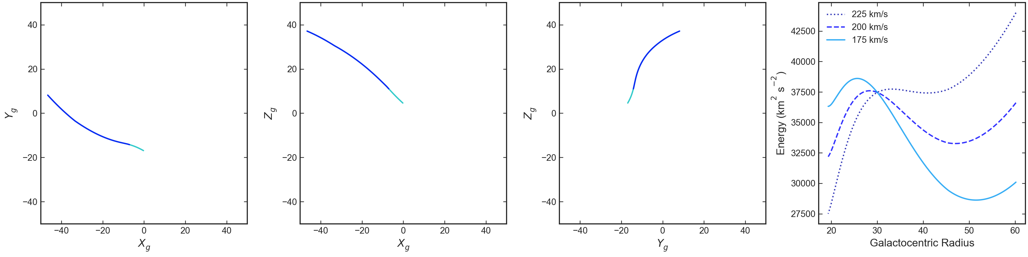
Figure 9: Left three panels: track of the stream in Galactocentric coordinates. The darker blue line shows the portion of the track $-35\degr<\Lambda<40\degr$ where all 6 dimensions are constrained, while the short, light blue continuation $40\degr<\Lambda<70\degr$ is the interval lacking radial velocity constraints. Here the Sun is at $X_{g}=8.12\,\mbox{kpc}$, $Y_{g}=Z_{g}=0$. Right panel: total energy of the stream as a function of Galactocentric radius, calculated using the six-dimensional track, and assuming logarithmic halo potentials with three different circular velocities. The potential is normalized to zero at $r=30\,\mbox{kpc}$.

The 6d track we have obtained enables us to examine the physical properties of the Orphan Stream. We keep this investigation brief since the near future will probably bring further significant information on the stream. It is not clear the full extent in longitude of the stream has been detected, and follow-up spectroscopy of likely stream targets should specify the velocity track over a greater longitude range.

In Figure 9, we plot our empirical track of the Orphan Stream in Galactocentric coordinates. Here we assume a distance to the Galactic center of $8.12\,\mbox{kpc}$ (Gravity Collaboration et al., 2018). We define $X_{g}$ so that it increases from the Sun to the Galactic center, in the same direction as Galactic $X$. The currently detected portion of the stream is a curving track over $60\,\mbox{kpc}$ long which approaches the disk plane at its southern extremity. A twist in this closest portion is apparent in these panels, though this part of the track is particularly uncertain due to sparse distance tracers and heavy contamination from the disk.

A tidal stream consists of stars moving with similar though not exactly constant energies. In the last panel of Figure 9, we plot the energy of the stream versus Galactocentric radius, assuming logarithmic halo potentials of three different circular velocities. The zero-point of the potential is set at $30\,\mbox{kpc}$. We see that the variance of the inferred energy is minimized at about $200\,\mbox{km}\,\mbox{s}^{-1}$, suggesting an outer Galactic rotation curve of about that level. While this is only a crude test, this value is in good agreement with various models of Galactic potential (Bland-Hawthorn & Gerhard, 2016), and in particular with recent results using  data on various tracers (Watkins et al., 2018; Posti & Helmi, 2018; Wegg et al., 2018; Vasiliev, 2018). We note that there is still a substantial wiggle in the energy versus radius, and it seems unlikely we could choose a simple potential where the energy could be made constant.

We fit several orbits to the observed stream track, using a fixed Galactic potential. The main goal here is not parameter fitting, because we know that streams have systematic departures from orbits (Johnston, 1998; Eyre & Binney, 2011), and thus we do not aim for statistical rigor. Rather, we want to look for systematic differences between the stream and the fitted orbits. We fitted our orbits to our derived stream tracks at a set of points spaced equally in longitude, rather than directly fitting the data. We assigned rough uncertainties of $\sim\!1/2$ the selection window in each observed dimension to govern the fits.

Three example orbits are listed in Table 1. In orbit 1 we combine the solar position of $8.12\,\mbox{kpc}$ with the proper motion of the Galactic center $6.379\,\mbox{mas}\,\mbox{yr}^{-1}$ (Reid & Brunthaler, 2004), and the motion of the Sun relative to the local standard of rest $U=11.10\,\mbox{km}\,\mbox{s}^{-1}$, $V=12.24\,\mbox{km}\,\mbox{s}^{-1}$, and $W=7.25\,\mbox{km}\,\mbox{s}^{-1}$ (Schönrich et al., 2010). The potential consists of a Hernquist bulge, a Miyamoto-Nagai disk, and an Navarro-Frenk-White halo, as specified in the table caption.

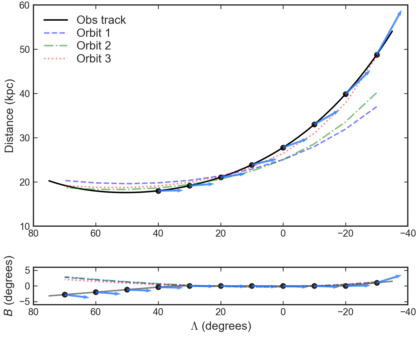
Figure 10: Comparison of the stream spatial track (black solid line) and local velocity vector (blue arrows). The three orbits in Table 1 are also shown. The unit galactocentric velocity vector is shown arbitrarily scaled for ease of visualization. Top: Distance versus longitude. The longitude range of the arrows is restricted to the interval probed by SDSS spectroscopy. A significant misalignment is seen, in that the velocity points less radially than the spatial track. Bottom: latitude versus longitude. The velocity arrows span the full latitude range of our track, since in this projection the radial velocity is not needed to compute their direction. Misalignment is mainly visible at large $\Lambda$ where the stream track bends to negative $B$. In both panels the velocity is computed using our smooth empirical tracks, and transformed to the galactocentric reference frame using our standard solar motion parameters (see text). If the stream track were an orbit, the arrows would point along the track.

Orbit 1 unsurprisingly comes much closer to matching the proper motion than the orbit 5 of Newberg et al. (2010), though some discrepancies remain. However, it is unable to fit the derived track in several respects. The most significant is that the distance does not reach values as large as in the observed stream, and the radial velocity is too high. The reason is simple: the spatial path of our derived stream track does not point in the same direction as its three-dimensional velocity vector, so it clearly cannot be modeled well by any orbit. The misalignment between the spatial path and velocity vector reaches approximately $20\degr$ in places. Figure 10 shows two projections, with the solid line representing our track and the arrows the direction of the local stream velocity after correcting for the solar reflex motion. As shown in the top panel, the stream path moves outward more rapidly along the direction of the stream’s motion (with $\Lambda$ decreasing) than one would expect from the velocity vector. In the bottom panel, the velocity does not point along our inferred path of the stream at large $\Lambda$ (the southern part of the stream). Our orbit fits also have difficulty in following the S-shaped path in latitude, and tend steadily towards larger $B$ at large $\Lambda$, rather than following the bend to negative values in our empirical track, as shown in the figure.

This misalignment was already somewhat apparent in the work of Hendel et al. (2018), even using the much smaller proper motion sample of Sohn et al. (2016). In that paper, samples of orbits constrained by the observations were obtained with and without the use of proper motion. Including proper motion pushed the derived orbits into the tail of the distributions obtained when it was omitted, indicating a significant level of tension. Our much more extensive proper motion dataset renders the level of disagreement far worse.

The inferred galactocentric velocity direction depends on the motion of the sun. If we allow some freedom in the solar motion, as in orbit 2, we can improve the fit to the observables somewhat. However, we find that good agreement between the track and an orbit is only obtained for implausible choices of the solar motion, requiring velocities differing by $>50\,\mbox{km}\,\mbox{s}^{-1}$ from currently preferred values and involving substantial motion out of the disk plane. In orbit 3 we instead force better agreement with the spatial track of the stream (again see Figure 10), at the cost of a $\sim\!30\,\mbox{km}\,\mbox{s}^{-1}$ disagreement with the observed radial velocity over a wide range in longitude. In these various fits the pericenter of the orbit is consistently about $17\,\mbox{kpc}$, as dictated by the spatial track, but the apocenter and orbital period are not well constrained.

It is not clear that a full dynamical model of the stream would necessarily reduce the misalignment we find here. In dynamical simulations the leading part of a tidal stream tends to lie inside the orbit, whereas the leading part of our observed track lies outside the fitted orbits. Other effects such as dynamical friction, or interactions with massive satellites such as Sagittarius or the LMC, may play a role in shaping the stream’s path. These effects are outside the scope of our preliminary investigation.

We note that we have tried various other potential forms, including bulge-disk-halo models with greater freedom in the halo properties, pure power-law potentials, and flat or cored logarithmic halo halo potential, with reasonable prolate or oblate halos. Overall, the detailed parameterization turns out to make little difference to the fitted orbital paths or the quality of the fits, perhaps because of the relatively short portion of the orbit sampled by the stream. The one property of the potential that seems to be well constrained by the fits is the circular velocity, or equivalently the radial acceleration or enclosed mass, in the range of radii probed by the stream (cf. Bonaca & Hogg, 2018). Not surprisingly, we find circular velocity values similar to those suggested by Figure 9.

Although our main focus has been on the central track of the stream, the widths of the stream in the coordinate dimensions also convey useful physical information. Constraining these widths is difficult due to observational errors, contamination, the likely non-Gaussian profiles of the stream, and possible substructure or other deviations from a smooth, constant-width stream. We have thus not attempted a rigorous computation of any of the dispersions. Nevertheless, over the interval $0\degr<\Lambda<50\degr$ at least, the stream appears fairly narrow in all coordinates. In Section 2 we estimated $\sigma_{B}\approx 1.3\degr$, $\sigma_{v}\approx 7\,\mbox{km}\,\mbox{s}^{-1}$, and $\sigma_{DM}\loa 0.2$ mag. We can compare these to the estimates of Hendel et al. (2018) based on a sample of RR Lyrae: $\sigma_{B}\approx 1.0\degr$, $\sigma_{v}\approx 30\,\mbox{km}\,\mbox{s}^{-1}$, and $\sigma_{DM}\approx 0.22$ mag. The samples are not entirely equivalent due to our proper-motion cleaning, which eliminates some of the outliers, and we have not chosen the same portion of the stream to estimate the widths. Furthermore, the much larger velocity dispersion in the RR Lyrae sample may be due in part to incomplete correction for the effects of radial pulsations.

Hendel et al. (2018) used a series of simulations matching their best-fit orbit and varying in progenitor mass to interpret their derived dispersions. (As these were one-component simulations, this progenitor mass corresponds only to the dense portion mixed with the stars that can survive the initial phases of tidal stripping.) The width in latitude pointed to a low progenitor mass ($<3\times 10^{7}\,M_{\odot}$), while the distance and velocity dispersions pointed to a high mass, $\sim\!3\times 10^{9}\,M_{\odot}$. To reconcile these, they suggested that the latitude width apparent in maps of main-sequence stars could be underestimated due to the background population. A dispersion of $\approx 2.5\degr$ would be required to be consistent with their high preferred progenitor mass.

With proper motion selection, the contamination we find in the central portion of the stream (see Figure 8) is low enough that a dispersion of this size seems unlikely. Instead, we suggest that the small dispersions in latitude and velocity together with the trends found by Hendel et al. (2018) point to a much lower progenitor mass of $\sim\!10^{8}\,M_{\odot}$. Meanwhile, the distance dispersion is sensitive to the assumed precision of observational distance estimates, the exclusion of outliers, and the longitude range used to compute the dispersion. We would not be surprised by a true distance modulus dispersion as low as $\sim\!0.1$ mag, consistent with a mass $\sim\!10^{8}\,M_{\odot}$.

All these quantitative assessments of the progenitor are of course quite imprecise, given the lack of an accurate and well-constrained model for the stream and the many possible sources of observational or theoretical error. Even so, the smaller mass we prefer may be easier to reconcile with the low mean metallicities of the Orphan Stream stars. For example, Draco, Ursa Minor, and Sextans were the three dSph we used as proxies for the Orphan progenitor in Section 2.2 due to their similar metallicity. These have dynamical masses within the half-light radius of only $10^{7}\,M_{\odot}$, $10^{7}\,M_{\odot}$, and $3\times 10^{7}\,M_{\odot}$ respectively (McConnachie, 2012).

4 CONCLUSIONS

We have used data from  DR2 and other surveys to constrain the properties of the Orphan Stream, over the entire region where it has previously been detected. We have clearly detected the proper motion of the stream over more than $90\degr$ in longitude. This result verifies and greatly extends an earlier detection using HST data (Sohn et al., 2016). We confirm and slightly update the previously obtained tracks of distance and velocity, with much lower ambiguity due to unrelated stars. Although increased contamination near the disk makes detection more difficult, we find evidence that the spatial path of the stream deviates from a great circle by about $2\degr$ in that area. Proper motion cleaning of previous spectroscopic surveys narrows, but does not eliminate, the metallicity dispersion in the stream. Consistent with this, the stream component exhibits a narrow red giant branch in the color-magnitude diagram. The low metallicity and small dispersions in the various observational dimensions suggest a progenitor of mass $\sim\!10^{8}\,M_{\odot}$.

The motion of the stream suggests a circular velocity of about $200$–$220\,\mbox{km}\,\mbox{s}^{-1}$ at $30\,\mbox{kpc}$, consistent with results using other tracers. Otherwise, the inferred behavior of the stream is not strongly sensitive to the form of the Galactic gravitational potential. The stream path deviates in significant ways from the behavior of an orbit; in particular, it does not point in the same direction as the 3d velocity vector. These apparent deviations can be reduced by shifts in the assumed solar motion, but optimum agreement requires unreasonable solar parameters. More work will be needed to constrain the total extent of the stream and understand its dynamics. We anticipate significant observational progress in the near future from further data mining of  and other surveys, future  releases, and targeted followup of stars along the stream.

Table 1: Orbits roughly matching the Orphan Stream. Kinematic properties (latitude $B_{0}$, distance $d_{0}$, proper motion in stream coordinates $\mu_{\Lambda,0}$ and $\mu_{B,0}$, and heliocentric radial velocity $v_{0}$) are specified at longitude $\Lambda=20\degr$. Orbits are integrated in a potential consisting of a Hernquist bulge with $M_{b}=4.5\times 10^{9}\,M_{\odot}$ and $a_{b}=0.44\,\mbox{kpc}$, a Miyamoto-Nagai disk with $M_{d}=6.8\times 10^{10}\,M_{\odot}$, $a_{d}=3.0\,\mbox{kpc}$, and $b_{d}=0.28\,\mbox{kpc}$, and a Navarro-Frenk-White halo parameterized as $\rho(r)=M_{h}/(4\pi r_{h}^{3})(r/r_{h})^{-1}(1+r/r_{h})^{-2}$. Solar motion parameters are relative to the Galactic center. Here latitude is in degrees, distance in  kpc, velocities in $\,\mbox{km}\,\mbox{s}^{-1}$, mass in $10^{11}\,M_{\odot}$, and proper motion in $\,\mbox{mas}\,\mbox{yr}^{-1}$.

Orbit	$B_{0}$	$d_{0}$	$\mu_{\Lambda,0}$	$\mu_{B,0}$	$v_{0}$	$M_{h}$	$r_{h}$	$v_{\odot,x}$	$v_{\odot,y}$	$v_{\odot,z}$
1	$-0.181$	$21.37$	$-1.372$	$-1.403$	$242.1$	$6.06$	$16$	$11.10$	$245.24$	$7.25$
2	$-0.138$	$20.63$	$-1.371$	$-1.384$	$238.3$	$4.98$	$16$	$11.57$	$222.26$	$13.96$
3	$-0.131$	$21.30$	$-1.260$	$-1.348$	$247.0$	$3.13$	$16$	$17.04$	$223.78$	$12.87$

References

- Astropy Collaboration et al. (2018) Astropy Collaboration et al., 2018, AJ, 156, 123
- Belokurov et al. (2006) Belokurov V., et al., 2006, ApJ, 642, L137
- Belokurov et al. (2007) Belokurov V., et al., 2007, ApJ, 658, 337
- Bland-Hawthorn & Gerhard (2016) Bland-Hawthorn J., Gerhard O., 2016, Annual Review of Astronomy and Astrophysics, 54, 529
- Bonaca & Hogg (2018) Bonaca A., Hogg D. W., 2018, ApJ, 867, 101
- Casey et al. (2013) Casey A. R., Da Costa G., Keller S. C., Maunder E., 2013, ApJ, 764, 39
- Casey et al. (2014) Casey A. R., Keller S. C., Da Costa G., Frebel A., Maunder E., 2014, ApJ, 784, 19
- Chambers et al. (2016) Chambers K. C., et al., 2016, preprint, (arXiv:1612.05560)
- Choi et al. (2016) Choi J., Dotter A., Conroy C., Cantiello M., Paxton B., Johnson B. D., 2016, ApJ, 823, 102
- Deason et al. (2011) Deason A. J., Belokurov V., Evans N. W., 2011, MNRAS, 416, 2903
- Dotter (2016) Dotter A., 2016, ApJS, 222, 8
- Eyre & Binney (2011) Eyre A., Binney J., 2011, MNRAS, 413, 1852
- Gaia Collaboration et al. (2016) Gaia Collaboration et al., 2016, A&A, 595, A1
- Gaia Collaboration et al. (2018) Gaia Collaboration et al., 2018, A&A, 616, A1
- Gravity Collaboration et al. (2018) Gravity Collaboration et al., 2018, A&A, 615, L15
- Grillmair (2006) Grillmair C. J., 2006, ApJ, 645, L37
- Grillmair et al. (2015) Grillmair C. J., Hetherington L., Carlberg R. G., Willman B., 2015, ApJ, 812, L26
- Hendel et al. (2018) Hendel D., et al., 2018, MNRAS, 479, 570
- Johnston (1998) Johnston K. V., 1998, ApJ, 495, 297
- Lindegren et al. (2018) Lindegren L., et al., 2018, A&A, 616, A2
- Malhan et al. (2018) Malhan K., Ibata R. A., Martin N. F., 2018, MNRAS, 481, 3442
- McConnachie (2012) McConnachie A. W., 2012, AJ, 144, 4
- Newberg et al. (2010) Newberg H. J., Willett B. A., Yanny B., Xu Y., 2010, ApJ, 711, 32
- Posti & Helmi (2018) Posti L., Helmi A., 2018, arXiv e-prints, p. arXiv:1805.01408
- Reid & Brunthaler (2004) Reid M. J., Brunthaler A., 2004, ApJ, 616, 872
- Schlafly & Finkbeiner (2011) Schlafly E. F., Finkbeiner D. P., 2011, ApJ, 737, 103
- Schlegel et al. (1998) Schlegel D. J., Finkbeiner D. P., Davis M., 1998, ApJ, 500, 525
- Schönrich et al. (2010) Schönrich R., Binney J., Dehnen W., 2010, MNRAS, 403, 1829
- Sesar et al. (2013) Sesar B., et al., 2013, ApJ, 776, 26
- Sesar et al. (2017) Sesar B., Hernitschek N., Dierickx M. I. P., Fardal M. A., Rix H.-W., 2017, ApJ, 844, L4
- Sohn et al. (2016) Sohn S. T., et al., 2016, ApJ, 833, 235
- Vasiliev (2018) Vasiliev E., 2018, arXiv e-prints, p. arXiv:1807.09775
- Vickers et al. (2012) Vickers J. J., Grebel E. K., Huxor A. P., 2012, AJ, 143, 86
- Watkins et al. (2018) Watkins L. L., van der Marel R. P., Sohn S. T., Evans N. W., 2018, arXiv e-prints, p. arXiv:1804.11348
- Wegg et al. (2018) Wegg C., Gerhard O., Bieth M., 2018, arXiv e-prints, p. arXiv:1806.09635