Distributed Submodular Minimization over Networks:
a Greedy Column Generation Approach

Abstract

Submodular optimization is a special class of combinatorial optimization arising in several machine learning problems, but also in cooperative control of complex systems. In this paper, we consider agents in an asynchronous, unreliable and time-varying directed network that aim at cooperatively solving submodular minimization problems in a fully distributed way. The challenge is that the (submodular) objective set-function is only partially known by agents, that is, each one is able to evaluate the function only for subsets including itself. We propose a distributed algorithm based on a proper linear programming reformulation of the combinatorial problem. Our algorithm builds on a column generation approach in which each agent maintains a local candidate basis and locally generates columns with a suitable greedy inner routine. A key interesting feature of the proposed algorithm is that the pricing problem, which involves an exponential number of constraints, is solved by the agents through a polynomial time greedy algorithm. We prove that the proposed distributed algorithm converges in finite time to an optimal solution of the submodular minimization problem and we corroborate the theoretical results by performing numerical computations on instances of the $s$–$t$ minimum graph cut problem.

I Introduction

In this paper we consider a set of agents communicating only with neighboring agents over a possibly asynchronous and unreliable network, and aiming at solving the combinatorial optimization problem

$$\operatornamewithlimits{min\vphantom{p}}_{X\subseteq V}F(X),$$ (1)

where $F$ is a real valued set function defined over subsets $X$ of a finite ground set $V$. We work under the assumption that the function $F$ exhibits the property of submodularity, that, as we detail later, represents a diminishing return property.

Submodularity is a branch of combinatorial optimization addressing several applications in machine learning, computer vision, game theory, and control of complex systems [1, 2, 3, 4, 5, 6]. Moreover, minimization of submodular set functions plays a key role in combinatorial optimization since it can be considered the discrete counterpart of convex minimization. Indeed, submodular problems can be efficiently solved through combinatorial algorithms as well as continuous methods involving convex (continuous) reformulations of the original problem [7, 8, 9, 10]. For these two reasons, investigating submodular minimization over networks is of great interest. While significant work has addressed continuous optimization over networks, the same cannot be said regarding (submodular) combinatorial optimization.

Submodularity emerged as an important tool for several control problems in multi-agent systems. Actuator and sensor placement problems [11, 12], leader selection in multi-agent systems [13] and performance optimization of composite networks [14] are addressed as constrained submodular minimization or maximization problems. In these works, the submodular optimization is a centralized high-level step (solved via greedy algorithms) to obtain performance guarantees for the multi-agent system. Submodularity is also related to game theory, e.g., for the analysis of the core of convex cooperative games [5]. In [15], the authors propose a decentralized allocation process, defined over a network of players, for transferable utility games. They assume, as we do, that each agent knows only the sets involving the agent itself. In [16], a distributed, consensus based, allocation process is proposed. Recently, seminal works have moved in the direction of casting submodular optimization over networks and solving the problem in a distributed way. In [17], a submodular maximization problem with cardinality constraints is investigated. Paper [18] handles the design of communication structures maximizing the worst case efficiency of the well-known greedy algorithm for submodular maximization when applied over networks. In [19], a submodular maximization problem, subject to matroid constraints, is solved in a decentralized fashion by means of a greedy algorithm and applied to multi-robot allocation. The same set-up is investigated in [20]. In [21], a fully distributed algorithm is proposed to minimize the sum of local submodular functions over lattices and applied to motion coordination.

The main contribution of this paper is as follows. We propose and analyze a distributed optimization algorithm to solve a submodular minimization problem over asynchronous, unreliable, time-varying and directed networks. In the considered set-up, agents are able to evaluate the objective function only for those sets including the agent itself. We rely on a proper linear programming reformulation of the combinatorial problem, which involves a factorial number of variables. Since the dimensionality of the problem represents a significant bottleneck (also in a centralized set-up) we resort to (a distributed version of) the well-known column generation approach, as in [22]. Differently form [22], in the proposed set-up each agent has to deal with an exponential number of local constraints. Thus, generating a column by directly solving the pricing problem would be computationally unaffordable. By explicitly taking into account submodularity, we design an efficient distributed column generation algorithm, ispired by [22], where agents are endowed with a local greedy algorithm that allows them to efficiently implement the column generation. The distributed algorithm works over unreliable, asynchronous, time-varying and directed networks and is shown to converge in finite time to an optimal set solution of the original submodular problem.

We highlight the main differences with [21]. Rather than considering a sum of cost functions fully computable by the agents, we consider a set-up in which each agent knows part of the domain, and a subset of values of the submodular function. Moreover, we prove finite time convergence to an optimal solution of the problem.

The paper unfolds as follows. Preliminaries about submodular optimization and a motivating example are presented in Section II. In Section III we describe the (centralized) column generation approach to solve submodular minimization. In Section IV we present our novel distributed algorithm for submodular minimization and its convergence properties. Numerical computations for the $s$–$t$ minimum cut problem are given in Section V.

Notation

$\mathbf{1}_{d}$ and $\mathbf{0}_{d}$ denote vectors in ^d with all entries equal to $1$ and $0$, respectively. The $\ell$-th entry of a vector $w$ is denoted by $(w)_{\ell}$. Let $V$ be a finite, non-empty set with cardinality $|V|$, also referred to as ground set. We denote by $2^{V}$ its power-set, i.e., the set of all its $2^{|V|}$ subsets. Given a set $X\subseteq V$, we denote by $\mathbf{1}_{X}\in^{|V|}$ its indicator vector defined as $(\mathbf{1}_{X})_{\ell}=1$ if $\ell\in X$, and $0$ if $\ell\not\in X$. Given $w\in^{|V|}$, we use the notation $w(X)=\mathbf{1}_{X}^{\top}w=\sum_{\ell\in X}(w)_{\ell}$.

II Submodular Minimization: Motivating Example and Preliminaries

In this section we introduce a motivating example of submodular minimization. Then, we recall the notion of submodular function and some properties. We also recall an equivalent continuous problem needed in our framework.

II-A Motivating Example: the Selection Problem

We introduce a motivating example of submodular minimization that is of interest in decision making in multi-agent network systems. Consider a set $V$ of teams. Each team has several skills at different levels that can be used in the accomplishment of a complex job. In a cooperative environment, teams collaborate to select the best subset of teams that maximizes the earning for the job of interest. In a distributed scenario each team is aware only of partial information regarding how much benefit can provide when involved in the job. Specifically, each team $i\in V$ knows a return value $r(i)$ obtained if team $i$ is selected for the job. Also, aggregating teams and combining their capabilities can result in a higher profit, while not doing it may result in a loss. Thus, each team $i$ knows also the value of a penalty $p(i,j)\geq 0$, for $i,j\in V$, strictly positive if $i$ is selected but $j$ is not. Thus, one obtains the set function

$$R(X)=\textstyle\sum\limits_{i\in X}r(i)-\textstyle\sum\limits_{\begin{subarray}{c}{i\in V}\\ {j\in V\setminus X}\end{subarray}}\!\!p(i,j),$$

which can be shown to be supermodular, i.e., $F(X)=-R(X)$ is submodular. Thus, the goal is to solve the problem $\operatornamewithlimits{max\vphantom{p}}_{X\subseteq V}R(X)$. This maximization of a supermodular function can be recast into an equivalent structured submodular minimization problem known as $s$–$t$ Min Cut problem, [5]. Such problem arises in several applications in Machine Learning, Decision Making and Signal Processing.

II-B Preliminaries on Submodular Minimization

A function $F:2^{V}\rightarrow$ is said to be submodular if, for all $A\subseteq V$ and $B\subseteq V$ the following condition holds, [8],

$$F(A)+F(B)\geq F(A\cup B)+F(A\cap B).$$

An alternative definition, which highlights the diminishing marginal returns property of submodular functions, follows. For all $A,B\subseteq V,\;A\subseteq B$, and for all $j\in V\setminus B$, then

$$F(A\cup j)-F(A)\geq F(B\cup j)-F(B).$$

This means that the incremental value made by a single element when added to an input set decreases as the size of the input set increases. Without loss of generality, we can consider a normalized function, i.e., such that $F(\emptyset)=0$.

Next, we define two polyhedra in ^|V|, respectively the submodular polyhedron and the base polyhedron, associated to submodular functions [8]. Given a submodular set function $F:2^{V}\rightarrow$, the associated submodular polyhedron is

$$P(F):=\{x\in^{|V|}\mid x(S)\leq F(S),\forall S\in 2^{V}\}.$$

Given $P(F)$, the base polyhedron associated to $F$ is

$$B(F):=\{x\in P(F)\mid x(V)=F(V)\}.$$ (2)

The set $B(F)$ is nonempty and bounded.

These two polyhedra are characterized by an exponential number of constraints, respectively $2^{|V|}-1$ and $2^{|V|}$. In Figure 1 the submodular and base polyhedra are depicted for a submodular function $F$ with ground set $V=\{1,2\}$.

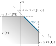
Figure 1: Example of $P(F)$ (shaded gray area) and $B(F)$ (blue segment) for a submodular function $F$ with ground set $V=\{1,2\}$.

Now, we show how a submodular function can be minimized by solving an equivalent continuous optimization problem over the base polyhedron. Let $F:2^{V}\rightarrow$, $F(\emptyset)=0$, be a submodular set function. Then as shown in [7], problem (1) has the same optimal cost of

$$\operatornamewithlimits{max\vphantom{p}}_{x\in B(F)}\textstyle\sum\limits_{\ell=1}^{|V|}\operatornamewithlimits{min\vphantom{p}}\{(x)_{\ell},0\}.$$ (3)

III A Column Generation Approach for Submodular Minimization

In this section we describe how a column generation method, based on Dantzig-Wolfe decomposition [23], can be applied to problem (3). Specifically, (3) is recast into a linear program (LP) in standard form for which (exploiting the “submodular nature”) column generation can be performed by means of an efficient greedy maximization algorithm.

Let $G\in^{|V|\times m}$ be a matrix whose columns are the vertexes of $B(F)$ (which are at most $|V|!$). Since $B(F)$ is bounded, then each element $x\in B(F)$ can be expressed as a convex combination of its vertexes. That is, we can write $x=G\,\theta$ where the coefficients $\theta\in^{m}$ satisfy $\mathbf{1}_{m}^{\top}\theta=1$, $\theta\geq 0$. Expressing $x$ as the difference of two positive vectors, namely $\alpha,\beta\in^{|V|}$, we can write $G\,\theta=\alpha-\beta$. Following [7], problem (3) can be recast as

$$\begin{split}\operatornamewithlimits{min\vphantom{p}}_{\theta,\alpha,\beta}\>&\>\mathbf{1}_{|V|}^{\top}\beta\\ \text{subj. to}\>&\>G\,\theta-\alpha+\beta=\mathbf{0}_{|V|}\\ &\>\mathbf{1}_{m}^{\top}\theta=1\\ &\>\alpha\geq\mathbf{0}_{|V|},\>\beta\geq\mathbf{0}_{|V|},\>\theta\geq\mathbf{0}_{m}.\end{split}$$ (4)

Let $(\theta^{\star},\alpha^{\star},\beta^{\star})$ be an optimal solution of (4), and let $(u^{\star},v^{\star})$ be the dual solutions associated to the equality constraints, with $u^{\star}$ being the one associated to $G\,\theta-\alpha+\beta=\mathbf{0}_{|V|}$. Then, $u^{\star}$ can be proven to have entries equal to $0$ or $1$. Specifically, $u^{\star}=\mathbf{1}_{X^{\star}}$ is the indicator vector of some optimal solution $X^{\star}\subseteq V$ of (1).

Notice that, in general, the solution of (4) is not unique. This comes from the non-uniqueness of the solution of (1). In particular, dual solutions associated to different primal solutions of (4) correspond to different minima of (1). This well-known degeneracy issue shall be carefully addressed in the distributed framework to be sure that agents agree on a common optimal set of the original submodular problem.

III-A The Reduced Problem and the Pricing Problem

The LP (4) has few constraints but a large number of variables. Thus, it can be tackled by a column generation approach. The first step is to solve a reduced instance of (4)

$$\begin{split}\operatornamewithlimits{min\vphantom{p}}_{\theta_{R},\alpha,\beta}\>&\>\mathbf{1}_{|V|}^{\top}\beta\\ \text{subj. to}\>&\>G_{R}\,\theta_{R}-\alpha+\beta=\mathbf{0}_{|V|}\\ &\>\mathbf{1}_{R}^{\top}\theta_{R}=1\\ &\>\alpha\geq\mathbf{0}_{|V|},\>\beta\geq\mathbf{0}_{|V|},\>\theta_{R}\geq\mathbf{0}_{R},\end{split}$$ (5)

where $G_{R}$ is a matrix with a smaller set of columns than $G$, so that the problem has a smaller decision vector $\theta_{R}$.

Let $\widetilde{z}=(\widetilde{\theta}_{R},\widetilde{\alpha},\widetilde{\beta})$ be an optimal solution of (5), and $(\widetilde{u},\widetilde{v})$ be the dual solutions associated to the constraints $G_{R}\,\theta_{R}-\alpha+\beta=\mathbf{0}_{|V|}$ and $\mathbf{1}_{R}^{\top}\theta_{R}=1$, respectively. A notable property of $\widetilde{u}$ is that $(\widetilde{u})_{\ell}=0$ if $(\widetilde{z})_{\ell}=(\widetilde{\alpha})_{k}$, and $(\widetilde{u})_{\ell}=1$ if $(\widetilde{z})_{\ell}=(\widetilde{\beta})_{k}$ (i.e., if the $\ell$-th component of $\widetilde{z}$ is associated to a component $k$ of $\widetilde{\alpha}$ or $\widetilde{\beta}$ respectively), see [7] for details.

With the dual solution $\widetilde{u}$ at reach, the next step consists in modifying $G_{R}$ in order to encode additional information about the optimal solution of the original problem. This procedure makes use of the so-called pricing problem, [23]. Here, a new column is generated by solving the LP, [10],

$$x^{B}\in\mathop{\rm argmax}_{x\in B(F)}\>(\widetilde{u})^{\top}x,$$ (6)

and defining the new column as $h_{\textsc{gen}}=[0\;\;(x^{B})^{\top}\;\;1]^{\!\top}$. The column generation algorithm proceeds by testing if the new generated column $h_{\textsc{gen}}$ allows for a cost improvement. This happens if its reduced cost is negative, i.e., if $(\widetilde{u})^{\top}x^{B}-\widetilde{v}<0$. In this case, the set of columns $G_{R}$ is enlarged by appending the column $h_{\textsc{gen}}$.

The algorithm iterates until $h_{\textsc{gen}}$ has non-negative reduced cost, which means that an optimal solution has been found. Given an optimal solution, the recover of an optimal solution of the submodular minimization problem (1) is obtained by looking at the dual variable $\widetilde{u}$. Indeed, $\widetilde{u}$ is the dual solution of (4), and, thus, it is the indicator vector of a solution of (1).

III-B Greedy Algorithm For Generating Columns

It is worth noticing that the maximization problem (6) involves an exponential number of constraints describing the base polyhedron $B(F)$. By explicitly relying on the structure of the problem, a greedy algorithm can be used to tackle the computational complexity of (6) allowing for a solution in a polynomial number of evaluations of $F$, [7].

For a generic instance of (6) with cost vector $\widetilde{u}\in^{|V|}$, the greedy algorithm consists of two steps. First, the components of $\widetilde{u}$ are reordered, by means of a sorting algorithm, so that index permutation $\{j_{1},\ldots,j_{|V|}\}$ satisfies $\widetilde{u}_{j_{1}}\geq\widetilde{u}_{j_{2}}\geq\ldots\geq\widetilde{u}_{j_{|V|}}$. Then, an optimal solution $x^{B}$ of (6) is given by

$$\big{(}x^{B}\big{)}_{j_{\ell}}\!\!=\!\begin{cases}F(\{j_{1}\}),&\text{if }\ell=1\\ F(\{j_{1}\ldots j_{\ell}\})\!-\!F(\{j_{1}\ldots j_{\ell-1}\}),\!\!&\text{if }2\leq\ell\leq N\!.\end{cases}$$

It is worth noting that each vertex of $B(F)$ corresponds to at least one permutation of the indexes $\{j_{1}\ldots j_{|V|}\}$, so that all optimal vertexes can be found by the greedy algorithm.

Remark III.1

The sorting of $\widetilde{u}$ is typically not unique. This translates into different vertexes of $B(F)$ with same optimal cost. Our distributed algorithm takes advantage from this non-uniqueness in the design of a local greedy algorithm using only local information. $\square$

IV Distributed Set-up and Column Generation Algorithm for Submodular Minimization

We now introduce our distributed optimization algorithm to solve a submodular minimization problem in the form (1). Then, we show its finite-time convergence.

IV-A Distributed Submodular Minimization Set-up

We consider $N=|V|$ agents in a network that aim at cooperatively solving a submodular minimization problem in the form (1). In our distributed set-up, we consider a scenario in which each agent $i$ is associated to element $i$ of $V$ and knows only the value of $F$ associated to all subsets of $V$ (in the power-set $2^{V}$) containing the element $i$ itself. Thus, agent $i$ ignores the information about all the other agents, i.e., $i$ knows $F(\{i\})$, does not know the value $F(\{j\})$ of a neighbor $j$, but both $i$ and $j$ know $F(\{i,j\})$.

Agents can exchange information according to a time-varying communication network modeled as a time-varying digraph $\mathcal{G}(t)=(\{1,\ldots,N\},E(t))$, with $t\in{\mathbb{N}}$ being a universal slotted time unknown to the agents. A digraph $\mathcal{G}(t)$ models the communication in the sense that there is an edge $(i,j)\in E(t)$ if and only if agent $i$ is able to send information to agent $j$ at time $t$. For each node $i$, the set of in-neighbors of $i$ at time $t$ is denoted by $\mathcal{N}^{\textrm{{in}}}_{i}(t)$ and is the set of $j$ such that there exists an edge $(j,i)\in E(t)$. The communication graph satisfies the following assumption.

Assumption IV.1 (On the network connectivity)

The time-varying graph $\mathcal{G}(t)$ is jointly strongly connected, i.e., $\forall t\in{\mathbb{N}}$, the graph $(\{1,\ldots,N\},\cup_{\tau=t}^{\infty}E(\tau))$ is strongly connected. $\square$

IV-B Local Greedy Algorithm

In this subsection we propose a variation of the greedy algorithm discussed in Section III-B that will be used to implement the column generation in a distributed fashion. Specifically, since agent $i$ is aware only of $F(X)$ with $X$ containing $i$, it may not be able to apply the greedy algorithm as introduced in Section III-B.

We recall that, given an input vector $u\in^{N}$, we need to order its components. However, agent $i$ can apply the greedy algorithm only if $j_{1}=i$, since otherwise would need to evaluate $F$ for sets not containing itself (e.g., $\{j_{1}\}$). Nonetheless, since the ordering $\{j_{1}\ldots j_{N}\}$ is not unique, we propose a priority-based sorting of the vector. That is, agent $i$ checks whether $(u)_{i}=\operatornamewithlimits{max\vphantom{p}}\{u\}$, i.e.,$(u)_{i}$ is the maximum entry of $u$. If so, it sets $j_{1}=i$ so that $\{j_{1},j_{2}\ldots j_{\ell}\}=\{i,j_{2}\ldots j_{\ell}\}$. We denote such a prioritized sorting routine by $\textsc{Sort}(u,i)$. Then, agent $i$ computes an optimal solution $x^{B}$ of the pricing problem for a given $u$ only if $(u)_{i}=\operatornamewithlimits{max\vphantom{p}}\{u\}$. In this case, it generates a new column as $h_{\textsc{gen}}=[0,(x^{B})^{\top},1]^{\top}$. Otherwise, it generates an empty column $h_{\textsc{gen}}=\texttt{null}$. This local procedure, called Local Greedy, is summarized in the following table.

Input: $u$, $i$

 Obtain an order via

$$\{j_{1},\ldots,j_{N}\}=\textsc{Sort}(u,i)$$

  if: $j_{1}=i$; then:

    Compute a new vertex $x^{B}$ as

$$\big{(}x^{B}\big{)}_{j_{\ell}}\!\!=\!\begin{cases}F(\{i\}),&\text{if }\ell=1\\ F(\{i\ldots j_{\ell}\})\!-\!F(\{j_{1}\ldots j_{\ell-1}\}),\!\!&\text{if }2\leq\ell\leq N\end{cases}$$

    Generate a new column as $h_{\textsc{gen}}=[0\;\;(x^{B})^{\top}\;\;1]^{\!\top}$

  else: $h_{\textsc{gen}}=\texttt{null}$

Output $h_{\textsc{gen}}$

Local Greedy Local Greedy Column Generation Algorithm

The Local Greedy is a local version of the (centralized) greedy algorithm described in Section III-B since it uses only local information at the node.

IV-C Greedy Distributed Column Generation Algorithm

In this subsection, we introduce our distributed algorithm for submodular minimization along with its convergence properties. Our methodology exploits the LP reformulation described in Section III combined with a distributed column generation approach.

Each agent $i$ maintains a local candidate basis $B^{[i]}(t)$ which is iteratively updated to eventually converge to the optimal basis of (4). Moreover, it maintains and updates dual variables $u^{[i]}(t)$ and $v^{[i]}(t)$ associated with the constraints in the local optimization problem. We will show that all $u^{[i]}(t)$ converge to a common indicator vector representing an optimal solution of the submodular minimization problem (1).

The algorithmic evolution is as follows. At every communication round $t$, agent $i$ receives from each neighbor $j\in\mathcal{N}^{\textrm{{in}}}_{i}(t)$ a matrix $G_{B}^{[j]}(t)$ containing those columns of $B^{[j]}(t)$ that are columns of $G$. Notice that a basis may also contain columns of the identity matrices associated to $\alpha$ and $\beta$. Then it collects all the columns of $G_{B}^{[j]}(t)$ $j\in\mathcal{N}^{\textrm{{in}}}_{i}(t)\cup\{i\}$ into a matrix $G^{[i]}(t)$, ordered according to a tie breaking rule. In particular, we use lexicographic ordering that guarantees uniqueness of the local basis for a given local problem. Compactly, we write $G^{[i]}(t)=\texttt{lexsort}(\cup_{j\in\mathcal{N}^{\textrm{{in}}}_{i}(t)\cup\{i\}}G_{B}^{[j]}(t))$. Then agent $i$ solves a reduced version of (4), i.e., a problem as (5) in which $G^{[i]}(t)$ is used in place of $G_{R}$. In particular, it computes the lexicographically optimal solution with corresponding basis $B^{[i]}(t)$ and corresponding dual variables $[u^{[i]}(t)^{\top},v^{[i]}(t)]^{\top}$. Then agent $i$ runs the Local Greedy routine described in Section IV-B on the vector $u^{[i]}(t)$ to (try to) generate a new column $h_{\textsc{gen}}^{[i]}$. Finally, agents perform a so-called pivoting operation, denoted by Pivot, in order to decide whether or not to include the new column in $B^{[i]}(t)$. Specifically, if the generated column $h_{\textsc{gen}}^{[i]}$ has negative reduced cost, then agent drops a column from the current basis $B^{[i]}(t)$ and introduces $h_{\textsc{gen}}^{[i]}$. Otherwise, the routine simply returns the previous basis. As for the LP solution, also the pivoting operation is performed by taking into account a lexicographic tie-breaking rule, see, e.g.,  [24].

At the first iterations, agents may not have knowledge of any column of $G$, and then be able to build a feasible local basis. For this reason, each agent initializes $G_{B}^{[i]}(0)$ with the solution $B_{H_{M}}$ of a local optimization problem on a set $H_{M}$ of artificial variables. That is, it considers $N+1$ decision variables with very high cost and solves an optimization problem depending on such variables and $\alpha$ and $\beta$ (where their cost is the same as in (4)). We point out that in this procedure, known as big-$M$ method, the artificial variables affect the solution only in the first iterations of the algorithm, and are dropped during its evolution. The distributed algorithm is formally reported in the following table from the perspective of node $i$.

Initialization: $G_{B}^{[i]}(0)=B_{H_{M}}$ obtained via big-$M$

Evolution: for all $t=1,2,\ldots$

 Receive $G_{B}^{[j]}(t)$ from $j\in\mathcal{N}^{\textrm{{in}}}_{i}(t)$ and set

$$G^{[i]}(t)=\texttt{lexsort}\Big{(}\cup_{j\in\mathcal{N}^{\textrm{{in}}}_{i}(t)\cup\{i\}}G_{B}^{[j]}(t)\Big{)}.$$

 Find optimal basis $B^{[i]}(t+1)$ with its corresponding

 dual optimal solution $[u^{[i]}(t)^{\top},v^{[i]}(t)]^{\top}$ of

$$\begin{split}\operatornamewithlimits{min\vphantom{p}}_{\theta_{R},\alpha,\beta}\>&\>\mathbf{1}_{|V|}^{\top}\beta\\ \text{subj. to}\>&\>G^{[i]}(t)\,\theta_{R}-\alpha+\beta=\mathbf{0}_{|V|}\\ &\>\mathbf{1}_{R}^{\top}\theta_{R}=1\\ &\>\alpha\geq\mathbf{0}_{|V|},\>\beta\geq\mathbf{0}_{|V|},\>\theta_{R}\geq\mathbf{0}_{R}.\end{split}$$ (7)

 Generate column $h_{\textsc{gen}}^{[i]}=\textsc{LocalGreedy}(u^{[i]}(t),i)$         $B^{[i]}(t+1)=\textsc{Pivot}\Big{(}B^{[i]}(t+1),h_{\textsc{gen}}^{[i]}\Big{)}$

 Construct $G_{B}^{[i]}(t+1)$ as columns of $G$ in $B^{[i]}(t+1)$

Distributed Algorithm Greedy Distributed Column Generation (GreeDiColumn)

We stress that our distributed algorithm is scalable in terms of local communication, computation and memory. Indeed, agents exchange at most $N+1$ columns from the local candidate basis. Thus, the computation complexity of (7) is always bounded by the number of in-neighbors. Also, each agent generates at most one new column at each communication round, and it stores only $B^{[i]}(t)$ and $[u^{[i]}(t)^{\top},v^{[i]}(t)]^{\top}$ ($N+1$ components). Thus, it is also memory efficient. Moreover, Assumption IV.1 models asynchronous communication and unreliable networks. Indeed, if a node is running its computation it is simply assumed not to have incoming and outgoing edges. Similarly, packet losses are modeled by neglecting (at a given time) those edges associated to packets not reaching the recipient. Finally, finite-time convergence allows agents to implement distributed stopping criteria as in [25].

We now provide a formal statement of the finite-time convergence of GreeDiColumn distributed algorithm to an optimal solution of the submodular minimization problem (1). The proof is omitted for the sake of space and will be provided in a forthcoming document.

Theorem IV.2

Let Assumption IV.1 hold and consider the sequences $\{B^{[i]}(t),u^{[i]}(t)\}_{t\geq 0}$, $i\in\{1,\ldots,N\}$ generated by GreeDiColumn. Then, in a finite number of communication rounds, say $T\in{\mathbb{N}}$, all the agents agree on a common optimal basis $B^{\star}$ corresponding to an optimal solution $(\theta^{\star},\alpha^{\star},\beta^{\star})$ of (4). Moreover, for all $t\geq T$ it holds

$$u^{[i]}(t)=\mathbf{1}_{X^{\star}},$$

for all $i\in\{1,\ldots,N\}$, being $X^{\star}$ an optimal solution of the submodular minimization problem (1). $\square$

V Numerical Computations

In this section we apply GreeDiColumn to a concrete example to numerically show its effectiveness.

V-A The $s$–$t$ Minimum Cut Problem

The $s$–$t$ Minimum Cut Problem arises as a key problem in several areas as machine learning, decision making and signal processing. It is, e.g., related to the maximum flow problem in a network, or to image segmentation (with nodes associated to pixels and edge capacities giving dissimilarity between two pixels), see [7, 3, 4, 5] and references therein.

Consider a static directed graph $\mathcal{G}_{st}=(V_{st},E_{st})$, where $V_{st}=\{s,t,1,\ldots N\}$ is the set of nodes and $E_{st}$ is the edge matrix. In particular, $s$ is called source node, and has only outgoing edges. Conversely, $t$ is called sink node, and has only incoming edges. A positive capacity $\kappa_{i,j}$ is associated to each edge $(i,j)\in E_{st}$.

A cut $U$ is a subset of $V_{st}$ that contains the source $s$ but does not contain the sink $t$. The cost of the cut is obtained by summing the capacities of the edges going from $U$ to $V_{st}\setminus U$. The goal is to find a $s$–$t$ minimum cut, i.e., a cut $U$ minimizing this cost. This problem can be cast as the following submodular minimization problem [8]. Let $V=V_{st}\setminus\{s,t\}$, then, for all $X\subseteq V$, define the function

$$F(X)=\!\!\textstyle\sum\limits_{\begin{subarray}{c}i\in X\\ j\in V\setminus X\end{subarray}}\!\!\kappa_{i,j}+\!\!\textstyle\sum\limits_{j\in V\cup\{t\}\setminus X}\!\!\kappa_{s,j}+\textstyle\sum\limits_{i\in X}\kappa_{i,t}-\!\!\textstyle\sum\limits_{j\in V\cup\{t\}}\!\!\kappa_{s,j}.$$

The first term takes into account the edges from $X$ to $V\setminus X$, the second one those from $s$ to $V\setminus X$ and (possibly) to $t$, and the third one those from $X$ to $t$. Finally, the last term guarantees that $F(\emptyset)=0$. The minimization of the function $F(X)$ over all subsets $X$ of $V$ gives an $s$–$t$ minimum cut as $U=X^{\star}\cup\{s\}$, with $X^{\star}$ being the minimum of $F$.

V-B Numerical Computations for the $s$–$t$ Min-Cut Problem

We consider a network of agents communicating according to a time-varying communication graph $\mathcal{G}(t)=(\{1,\ldots,N\},E(t))$ satisfying Assumption IV.1. Each agent $i$ of the network is associated to a node $i\in V$ of the $s$–$t$ min-cut graph, see Figure 2 for a graphical interpretation.

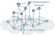
Figure 2: $s$–$t$ min-cut graph and its associated communication network. Only an instance of the (time-varying) communication graph is shown.

We generate random $s$–$t$ min-cut graphs by constructing Erdős-Rényi random graphs of $|V|$ nodes, with edges existence probability $0.1$. Source and sink nodes $s$ and $t$ are randomly attached to the other nodes with a discrete uniform probability. The edge capacities are fractional numbers, with one decimal digit, uniformly drawn in $[0.1,10]$. We analyze the performance of our algorithm in two different scenarios: $(i)$ a sequence of fixed (cycle) communication graphs with an increasing number of nodes, and $(ii)$ an unreliable network modeled as an underlying (random) fixed graph with packet losses. For comparison, we use the submodular optimization (centralized) toolbox in [26] to compute the optimal cost $J^{\star}$.

(i)

We analyze the performance of the proposed algorithm in terms of convergence steps, while varying the network size (in terms of diameter) as a function of the problem size. We consider $|V|=\{8,16,24,32,40,48\}$. For each case, we run $100$ instances. The communication graph is a cycle that has diameter equal to $d_{\mathcal{G}}=N-1=|V|-1$. The results are reported in Figure 3 (left). The red line in the center of each box is the median value of communication rounds needed for the convergence. Edges of the box represent the $25$-th and the $75$-th percentiles. The whiskers represents the most extreme data points not considered as outliers (marked with the red crosses). We highlight that the communication rounds needed for the convergence scales linearly with the problem size.

(ii)

We test the robustness of our algorithm when running over unreliable networks subject to packet losses. We consider the same random model introduced above for a network of $48$ nodes connected by a random graph with diameter $d_{\mathcal{G}}=9$. The same graph is used as “nominal” communication graph. In particular, at each communication round, the $i$-th agent discards the incoming message from the $j$-th agent according to a given, fixed probability of loss given by $\{10\%,30\%,50\%,90\%\}$. Figure 3 (right) shows the number of communication rounds necessary to converge to an optimal solution. Consistently with the theory, the algorithm converges to an optimal solution even with $90\%$ probability of losses. As expected, the convergence time increases as the packet loss probability increases.

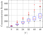
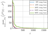
Figure 3: Left: communication rounds trend while increasing the network diameter $d_{\mathcal{G}}$ with the problem size ($d_{\mathcal{G}}=|V|-1$). Right: communication rounds to convergence with different loss probabilities.

VI Conclusions

In this paper, we proposed a distributed algorithm to minimize submodular functions over peer-to-peer networks, where an agent knows the function values only for those sets including itself. Exploiting the submodular structure and a linear program reformulation of the original problem, we designed a distributed column generation algorithm for submodular minimization. Agents are endowed with a local greedy procedure to generate columns without explicitly solving a pricing problem having exponentially many constraints. We showed the finite-time convergence of the distributed algorithm to an optimal solution of the submodular minimization problem. Numerical simulations corroborated the theoretical results.

References

- [1] K. Wei, R. Iyer, and J. Bilmes, “Submodularity in data subset selection and active learning,” in Int. Conf. on Machine Learning, 2015, pp. 1954–1963.
- [2] Z. Jiang, G. Zhang, and L. S. Davis, “Submodular dictionary learning for sparse coding,” in IEEE Conf. on Computer Vision and Pattern Recognition (CVPR), 2012, pp. 3418–3425.
- [3] P. Stobbe and A. Krause, “Efficient minimization of decomposable submodular functions,” in Adv. in Neural Inform. Proc. Sys., 2010, pp. 2208–2216.
- [4] S. Jegelka, F. Bach, and S. Sra, “Reflection methods for user-friendly submodular optimization,” in Adv. in Neural Inform. Proc. Sys., 2013, pp. 1313–1321.
- [5] D. M. Topkis, Supermodularity and complementarity. Princeton Univ. Press, 2011.
- [6] F. Bach, “Structured sparsity-inducing norms through submodular functions,” in Adv. in Neural Inform. Proc. Sys., 2010, pp. 118–126.
- [7] ——, “Learning with submodular functions: A convex optimization perspective,” Foundations and Trends® in Machine Learning, vol. 6, no. 2-3, pp. 145–373, 2013.
- [8] S. Fujishige, Submodular functions and optimization. Elsevier, 2005, vol. 58.
- [9] S. T. McCormick, “Submodular function minimization,” Handbooks in Operations Res. and Manag. Science, vol. 12, pp. 321–391, 2005.
- [10] A. Orso, J. Lee, and S. Shen, “Submodular minimization in the context of modern LP and MILP methods and solvers,” in Int. Symposium on Experimental Algorithms. Springer, 2015, pp. 193–204.
- [11] T. H. Summers, F. L. Cortesi, and J. Lygeros, “On submodularity and controllability in complex dynamical networks,” IEEE Trans. on Control of Network Systems, vol. 3, no. 1, pp. 91–101, 2016.
- [12] V. Tzoumas, A. Jadbabaie, and G. J. Pappas, “Sensor placement for optimal Kalman filtering: Fundamental limits, submodularity, and algorithms,” in IEEE Americ. Contr. Conf. (ACC), 2016, pp. 191–196.
- [13] A. Clark, L. Bushnell, and R. Poovendran, “A supermodular optimization framework for leader selection under link noise in linear multi-agent systems,” IEEE Trans. on Automatic Control, vol. 59, no. 2, pp. 283–296, 2014.
- [14] E. Mackin and S. Patterson, “Optimizing the coherence of composite networks,” in IEEE Americ. Contr. Conf. (ACC), 2017, pp. 4334–4340.
- [15] A. Nedić and D. Bauso, “Dynamic coalitional TU games: Distributed bargaining among players’ neighbors,” IEEE Trans. on Automatic Control, vol. 58, no. 6, pp. 1363–1376, 2013.
- [16] D. Bauso and G. Notarstefano, “Distributed -player approachability and consensus in coalitional games,” IEEE Trans. on Automatic Control, vol. 60, no. 11, pp. 3107–3112, 2015.
- [17] I. Bogunovic, S. Mitrovic, J. Scarlett, and V. Cevher, “A distributed algorithm for partitioned robust submodular maximization,” in IEEE Int. Workshop on Comp. Adv. in Multi-Sensor Adaptive Proc. (CAMSAP), 2017, pp. 1–5.
- [18] D. Grimsman, M. S. Ali, J. P. Hespanha, and J. R. Marden, “Impact of information in greedy submodular maximization,” in IEEE Conf. on Dec. and Control (CDC), 2017, pp. 2900–2905.
- [19] R. K. Williams, A. Gasparri, and G. Ulivi, “Decentralized matroid optimization for topology constraints in multi-robot allocation problems,” in IEEE Int. Conf. on Robotics and Autom. (ICRA), 2017, pp. 293–300.
- [20] B. Gharesifard and S. L. Smith, “Distributed submodular maximization with limited information,” IEEE Trans. on Control of Network Systems, vol. PP, no. 99, pp. 1–11, 2017.
- [21] H. Jaleel and J. Shamma, “Distributed submodular minimization and motion coordination over discrete state space,” arXiv preprint arXiv:1709.07379, 2017.
- [22] M. Bürger, G. Notarstefano, and F. Allgöwer, “Locally constrained decision making via two-stage distributed simplex,” in IEEE Conf. on Dec. and Control and European Control Conf. (CDC-ECC), 2011, pp. 5911–5916.
- [23] G. B. Dantzig and P. Wolfe, “Decomposition principle for linear programs,” Operations research, vol. 8, no. 1, pp. 101–111, 1960.
- [24] C. N. Jones, E. C. Kerrigan, and J. M. Maciejowski, “Lexicographic perturbation for multiparametric linear programming with applications to control,” Automatica, vol. 43, no. 10, pp. 1808–1816, 2007.
- [25] G. Notarstefano and F. Bullo, “Distributed abstract optimization via constraints consensus: Theory and applications,” IEEE Trans. on Automatic Control, vol. 56, no. 10, pp. 2247–2261, 2011.
- [26] A. Krause, “SFO: A toolbox for submodular function optimization,” J. of Machine Learning Res., vol. 11, no. Mar, pp. 1141–1144, 2010.