Renormalization group flows for Wilson-Hubbard matter and the topological Hamiltonian

Abstract

Understanding the robustness of topological phases of matter in the presence of interactions poses a difficult challenge in modern condensed matter, showing interesting connections to high energy physics. In this work, we leverage these connections to present a complete analysis of the continuum long-wavelength description of a generic class of correlated topological insulators: Wilson-Hubbard topological matter. We show that a Wilsonian renormalization group (RG) approach, combined with the so-called topological Hamiltonian, provide a quantitative route to understand interaction-induced topological phase transitions that occur in Wilson-Hubbard matter. We benchmark two-loop RG predictions for a quasi-1D Wilson-Hubbard model by means of exhaustive numerical simulations based on matrix product states (MPS). The agreement of the RG predictions with MPS simulations motivates the extension of the RG calculations to higher-dimensional topological insulators.

I Introduction

Condensed-matter and high-energy physics study phenomena at vastly different scales and, yet, these can often be understood by the same concepts and unifying principles. One of the major examples of the cross-fertilization of fundamental ideas between these two disciplines is the theory of spontaneous symmetry breaking, which is both paramount to our current understanding of phases and phase transitions in condensed matter landau ; landau_ginzburg ; anderson , and to the standard model describing elementary particles and their interactions nambu ; goldstone ; higgs . These parallelisms become clearer under the light of a common language: the theory of interacting quantum fields fradkin_book ; qft_book . In this context, again, a multi-disciplinar approach based on concepts of scaling and critical phenomena leads to the so-called renormalization group wk_rg , which has turned out to be the key to understand many-body effects in condensed-matter systems shankar_rg , or the very definition of a relativistic quantum field theory rg_conceptual .

Beyond these fruitful connections, there is also the possibility of finding condensed-matter analogues of models initially introduced in the realm of high-energy physics, or vice versa. In this way, one may not only use a common framework to understand widely different phenomena, but actually observe the same phenomenon in two different scenarios. Graphene is a representative and well-known example of this situation graphene_review , as the low-energy electronic excitations of this semi-metal act as analogues of a relativistic quantum field theory of massless Dirac fermions. Another recent example of this trend lies in the physics of topological insulators, which are insulating phases of matter that are not characterized by local order parameters but, instead, by certain topological invariants Bernevig . Some of these topological insulators can be represented by minimal models that are condensed-matter analogues of relativistic quantum field theories of massive Wilson fermions wilson_fermions , which originally appeared in the context of lattice gauge theories for elementary particle physics lattice_book .

A question of current interest in the field of topological insulators ti_interactions_reviews and symmetry-protected topological (SPT) phases spt_review is to explore correlation effects, such as the possibility of finding interaction-induced quantum phase transitions that separate these SPT phases from other non-topological ground-states. Let us note that, although these topological quantum phase transitions cannot be understood from the principle of spontaneous symmetry breaking mentioned above, they can still be characterized by the closure of a many-body energy gap, such that scaling phenomena should also be relevant. Accordingly, the connection of continuum relativistic quantum field theories (QFTs), scaling, and the renormalization group (RG) to these topological phases might offer a systematic route to understand correlation effects. In this paper, we carefully explore this possibility for certain types of correlated topological insulators: Wilson-Hubbard topological matter, which can be described in terms of a relativistic QFT of massive Wilson fermions with four-Fermi interactions in the vicinity of a topological band inversion point. We show that a Wilsonian RG offers a neat qualitative picture to understand these topological phases, and a quantitative scheme to obtain the phase boundaries that separate them from other non-topological phases.

This article is organized as follows. In Sec. II, we start by reviewing the use of relativistic QFTs of massive Wilson fermions as long-wavelength representatives of topological insulators II.1. We then include interactions leading to Wilson-Hubbard topological matter, and discuss the Euclidean functional integral that contains all relevant information about the possible phases and phase transitions II.2. In II.3, we start by reviewing the Wilsonian approach to the RG of interacting QFTs. We then move on to discuss generic features of the RG flows for Wilson-Hubbard matter at tree level, which offer a neat connection between the long-wavelength limit and the flat-band limit of topological insulators. We also discuss the use of the RG flows of the QFT parameters to obtain interaction-induced corrections to the so-called topological Hamiltonian self_energy_topological ; topological_hamiltonian , providing a straightforward route to calculate the corresponding many-body topological invariants. In Sec. III, we apply the RG to a one-dimensional model of Wilson-Hubbard matter: the imbalanced Creutz-Hubbard ladder III.1. This model of an interacting topological insulator yields a perfect playground to test the qualitative and quantitative validity of the RG approach beyond tree level, as one may compare two-loop RG corrections to quasi-exact numerical simulations based on matrix product states III.2. In III.3, we provide a further benchmark of the RG calculations and the renormalized topological Hamiltonian by characterizing the bi-partite correlations at the topological quantum phase transition. Finally, in Sec. IV, we present our conclusions and outlook.

II Functional integrals for topological insulators with Hubbard-type interactions

II.1 Quantum field theories as representatives of non-interacting topological insulators

In this section, we describe a generic lattice Hamiltonian TI_field_theories ; 10_fold_ryu ; wilson_atoms that can host different classes of non-interacting topological insulators review_top_insulators ; Bernevig , as well as a continuum quantum field theory that captures its long-wavelength properties, including the underlying topological features. This will serve us to review certain aspects of topological insulators, and to set the notation used throughout this manuscript.

(a) Continuum Dirac QFTs and topological invariants.–

A fundamental ingredient of this work is the massive Dirac quantum field theory in a $D=(d+1)$-dimensional Minkowski space-time qft_book , which can serve as a building block to construct a representative QFT for various topological insulating phases 10_fold_ryu . In the Hamiltonian formulation, this quantum field theory (QFT) can be written as

$$H_{\rm D}\!=\!\bigintssss_{{\Lambda}^{d}}\!\frac{{\rm d}^{d}k}{(2\pi)^{d}}\Psi_{\mu}^{\dagger}(\bm{k})[h_{\rm D}(\bm{k})]^{\mu,\nu}\Psi_{\nu}^{\phantom{\dagger}}(\bm{k}),\hskip 4.30554pth_{\rm D}(\bm{k})=\alpha_{i}\hskip 0.6458ptk^{i}+m\beta,$$ (1)

where $\Psi^{\phantom{\dagger}}\!\!\!\!(\bm{k}),\Psi^{{\dagger}}\!(\bm{k})$ are the spinor fermionic field operators fulfilling $\{\Psi_{\mu}^{\phantom{\dagger}}(\bm{k}),\Psi_{\nu}^{{\dagger}}(\bm{k}^{\prime})\}=(2\pi)^{d}\delta_{\mu,\nu}\delta^{(d)}(\bm{k}-\bm{k}^{\prime})$, and the momentum lies below a certain ultra-violet (UV) cutoff to regulate the QFT, namely $\bm{k}\in{\Lambda}^{d}$ if $|k_{i}|\leq\Lambda_{\rm c}$ (i.e. $\Lambda^{d}\to\mathbb{R}^{d}$ as the cutoff is removed $\Lambda_{\rm c}\to\infty$). In the above expression, $\{\alpha_{i}\}_{i=1}^{d}$ and $\beta$ are the so-called Dirac matrices, which are mutually anti-commuting Hermitian matrices that square to the identity, and we use natural units $\hbar=c=1$ together with Einstein’s summation criterion. Depending on the particular choice of the Dirac matrices rqm_book , the single-particle Hamiltonian $h_{\rm D}(\bm{k})$ may, or may not, respect the following discrete symmetries: time-reversal symmetry $\mathsf{T}$ is fulfilled if $U_{\mathsf{T}}h_{\rm D}(-\bm{k})^{*}U_{\mathsf{T}}^{\dagger}=h_{\rm D}(\bm{k})$; particle-hole symmetry $\mathsf{C}$ takes place when $U_{\mathsf{C}}h_{\rm D}(-\bm{k})^{*}U_{\mathsf{C}}^{\dagger}=-h_{\rm D}(\bm{k})$; and the so-called sub-lattice symmetry $\mathsf{S}$ occurs if $U_{\mathsf{S}}h_{\rm D}(\bm{k})U_{\mathsf{S}}^{\dagger}=-h_{\rm D}(\bm{k})$, where we have introduced various unitary rotations $U_{\mathsf{T}},U_{\mathsf{C}},U_{\mathsf{S}}$ table_top_insulators . We note that these discrete symmetries can be related to the ten-fold classification of symmetric spaces az_ten_fold via the corresponding time-evolution operator $U_{\rm D}(t)={\rm e}^{-{\rm i}th_{\rm D}(\bm{k})}$.

To give concrete examples that shall be used throughout this work, let us consider (i) the $(2+1)$-dimensional QFT (1) with $\alpha_{1}=\sigma^{x}$, $\alpha_{2}=\sigma^{y}$, and $\beta=\sigma^{z}$ expressed in terms of Pauli matrices. In this case, there is no unitary operator that can fulfill any of the above transformations, and the Dirac QFT thus explicitly breaks the time-reversal, particle-hole, and sub-lattice symmetries. In this case, the time-evolution operator $U_{\rm D}(t)={\rm e}^{-{\rm i}th_{\rm D}(\bm{k})}$ lies in the so-called unitary symmetric space 10_fold_ryu , labeled as $\mathsf{A}$. From this parent Hamiltonian, one may use a Kaluza-Klein-type dimensional reduction by compactifying the second spatial direction into a vanishingly small circle TI_field_theories ; 10_fold_ryu . (ii) The resulting $d=1$ Dirac QFT (1) with $\alpha_{1}=\sigma^{x}$, and $\beta=\sigma^{z}$, now respects the sub-lattice symmetry with $U_{\mathsf{S}}=\sigma^{y}$, but breaks both time-reversal and particle-hole symmetries. In this case, the time-evolution operator belongs to the chiral unitary symmetric space, labeled as $\mathsf{AIII}$. We note that this idea of dimensional reduction allows one to find representatives of all ten possible symmetric spaces starting from a higher-dimensional Dirac QFT TI_field_theories ; 10_fold_ryu .

To understand the use of these QFTs as building blocks of topological insulators, let us consider the zero-temperature groundstate $|\epsilon_{\rm gs}\rangle=\prod_{\bm{k}\in\Lambda^{d}}|\epsilon_{-}(\bm{k})\rangle$, which is obtained by occupying all the single-particle modes $|\epsilon_{-}(\bm{k})\rangle$ with energies $\epsilon_{-}(\bm{k})=-\sqrt{m^{2}+\bm{k}^{2}}$. Depending on the dimensionality and the discrete symmetries of the Hamiltonian introduced above, one can define a topological invariant that characterizes each ground-state. These topological invariants, which cannot be modified by perturbations that respect the corresponding symmetries unless a quantum phase transition takes place, can be defined through momentum integrals of either the so-called Chern characters or Chern-Simons forms 10_fold_ryu . For the examples cited above, one finds that: (i) the $d=2$ Dirac QFT in the $\mathsf{A}$ class is characterized by the integral of the first Chern character $\mathsf{ch}_{1}=\frac{{\rm i}}{2\pi}\partial_{k^{i}}\langle\epsilon_{-}(\bm{k})|\partial_{k^{j}}|\epsilon_{-}(\bm{k})\rangle dk^{i}\times dk^{j}$,

$$\mathsf{Ch}_{1}=\int_{\Lambda^{2}}\mathsf{ch}_{1}=\frac{m}{2|m|}.$$ (2)

This topological invariant, which is known as the first Chern number, cannot change unless $m=0$, which signals a quantum phase transition. (ii) For the $d=1$ Dirac QFT in the $\mathsf{AIII}$ class, the integral of the first Chern-Simons form $\mathsf{Q}_{1}=\frac{{\rm i}}{2\pi}\langle\epsilon_{-}({k})|\partial_{k}|\epsilon_{-}({k})\rangle dk$ yields the Chern-Simmons invariant

$$\mathsf{CS}_{1}=\int_{\Lambda^{1}}\mathsf{Q}_{1}=\frac{m}{4|m|}.$$ (3)

In contrast to the Chern number, this quantity is not gauge invariant, and one typically defines an associated Wilson loop $\mathsf{W}_{1}={\rm e}^{{\rm i}2\pi\mathsf{CS}_{1}}$, which gives a quantized topological invariant that cannot change unless $m=0$. We emphasize that similar topological invariants can be constructed for any particular higher-dimensional Dirac QFT 10_fold_ryu , which allows one to find the required building blocks for all 10 possible topological insulators-superconductors table_top_insulators , excluding the appearance of additional crystalline symmetries.

(b) Discretized QFTs, fermion doubling and invariants.–

From a condensed-matter perspective fradkin_book , the above Dirac QFT (1) will arise as a low-energy approximation that tries to capture the relevant physics of a particular material at long wavelengths $\xi\gg a$ or, equivalently, at low momenta $|{k_{i}}|\leq\Lambda_{\rm c}\ll 2\pi/a$. Here, $a$ is the lattice constant of the material, which serves as natural UV regulator of the QFT. Paradigmatic examples of massless Dirac QFTs in condensed-matter setups appear in the so-called one-dimensional Luttinger liquids LL_review and two-dimensional graphene graphene_review . On the other hand, for a non-vanishing mass/gap, these continuum QFTs (1) can serve as building blocks to construct a low-energy approximation of topological insulators. Let us now introduce some peculiarities of the lattice regularization from the perspective of lattice field theory (LFT) lattice_book .

A naive approach is to discretize the spatial derivatives of the Dirac Hamiltonian that lead to the linear dependence on momentum in Eq. (1). By introducing a Bravais lattice $\Lambda_{\ell}=a\mathbb{Z}^{d}=\{\bm{x}:x_{i}/a\in\mathbb{Z},\forall i=1,\cdots,d\}$, the corresponding Hamiltonian LFT can be expressed as follows

$$H_{\rm D}=\!\!\sum_{\bm{x}\in\Lambda_{\ell}}\!\!a^{d}\!\left(\!\Psi^{\dagger}(\bm{x})\frac{{\rm i}\alpha_{i}}{2a}\Psi\!\left(\bm{x}+a\bm{u}^{i}\right)+m\,\Psi^{\dagger}(\bm{x})\frac{\beta}{2}\Psi(\bm{x})+{\rm H.c.}\!\right)\!,$$ (4)

where $\{\bm{u}^{i}\}_{i=1}^{d}$ are the unit vectors of the Bravais lattice. Moreover, the lattice spinor fields $\Psi(\bm{x}),\Psi^{{\dagger}}\!(\bm{x})$ display the desired anti-commutation algebra in the continuum limit $\{\Psi_{\mu}^{\phantom{\dagger}}(\bm{x}),\Psi_{\nu}^{{\dagger}}(\bm{x}^{\prime})\}=\frac{1}{a^{d}}\delta_{\mu,\nu}\delta_{\bm{x},\bm{x}^{\prime}}\to\delta_{\mu,\nu}\delta^{(d)}(\bm{x}-\bm{x}^{\prime})$. Transforming the field operators to momentum space,

$$\Psi_{\mu}^{\phantom{\dagger}}(\bm{x})=\int_{{\rm BZ}^{d}}\!\frac{{\rm d}^{d}k}{(2\pi)^{d}}{\rm e}^{{\rm i}\bm{k}\cdot\bm{x}}\hskip 1.07639pt\Psi_{\mu}^{\phantom{\dagger}}(\bm{k}),$$ (5)

one obtains a QFT similar to Eq. (1), where momenta now lie within the so-called Brillouin zone $\Lambda^{d}\to{\rm BZ}^{d}=(-\frac{\pi}{a},\frac{\pi}{a}]^{\times^{d}}$, and the single-particle Hamiltonian is

$$h_{\rm D}(\bm{k})=\frac{1}{a}\alpha_{i}\sin(k^{i}a)+m\beta.$$ (6)

The energy spectrum of this lattice Hamiltonian becomes $\epsilon_{\pm}(\bm{k})\approx\pm\sqrt{m^{2}+\bm{k}^{2}}$ at long wavelengths $\xi\sim k_{i}^{-1}\gg a$, and thus reproduces the energy of the massive Dirac fermion. However, there are other points at the borders of the Brillouin zone that lead to a similar dispersion relation (i.e. Dirac points), and thus give rise to additional relativistic fermions, the so-called fermion doublers. In fact, there is an even number $N_{\rm D}=2^{d}$ of Dirac points, labelled by $\bm{k}_{\bm{n}}=\frac{\pi}{a}n_{i}\bm{u}^{i}$ with $n_{i}\in\{0,1\}$, which lead to a dispersion relation that is approximately described by a massive relativistic particle $\epsilon_{\pm}(\bm{k}_{\bm{n}}+\bm{k})\approx\pm\sqrt{m^{2}+\bm{k}^{2}}$ at long wavelengths $\xi\sim k_{i}^{-1}\gg a$. The effective QFT around each of these points corresponds to an instance of the massive Dirac QFT $h_{\rm D}(\bm{k}_{\bm{n}}+\bm{k})\approx\alpha_{i}^{\bm{n}}\hskip 0.6458ptk^{i}+m\beta$ with a different choice of the Dirac matrices $\alpha_{i}^{\bm{n}}=(-1)^{n_{i}}\alpha_{i}$. Let us note that this effective QFT is defined within a certain long-wavelength cutoff where the linearization is valid, such that $\Lambda^{d}=(-\pi/l_{\rm c},\pi/l_{\rm c}]^{\times^{d}}$ in Eq. (1). As will become clear below, using the perspective of the renormalization group (RG) wk_rg , we shall approach this continuum limit by setting the parameters of the lattice Hamiltonian close to a quantum phase transition, where the characteristic correlation length diverges $\xi/l_{\rm c}\to\infty$, and effectively ${\Lambda}^{d}\to\mathbb{R}^{d}$. Accordingly, we get $N_{\rm D}$ copies of the desired continuum QFT (1).

From the perspective of LFT, the presence of fermion doublers with $\bm{n}\neq 0$ is an unfortunate nuisance, as they will inevitably couple to the target $\bm{n}=0$ Dirac QFT as soon as additional interaction terms are included lattice_book . Moreover, the presence of the doublers is a generic feature for different lattice discretizations, and is related to the difficulty of incorporating chiral symmetry on the lattice nn_theorem .

From the perspective of topological insulators, the presence of these doublers is already important at the non-interacting level. In the lattice, the even number of relativistic fermions can be divided into two sets $S_{\pm}$ with opossite chiralities, each of which contains an equal number $|S_{\pm}|=2^{(d-1)}$of Dirac points: $\bm{n}\in S_{\pm}$ if $(-1)^{\sum_{i}n_{i}}=\pm 1$. This sign difference is translated into an opposite Chern character (2) or Chern-Simons form (3), such that the topological invariant obtained by integrating over the whole Brillouin zone vanishes (i.e. summing an equal number of positive and negative contributions over all Dirac points yields a zero topological invariant). Accordingly, due to the presence of the spurious fermion doublers, this naive lattice Hamiltonian (4) fails at reproducing the non-vanishing topological invariant in Eq. (2) or (3) of the single massive Dirac QFT (1). For the representative examples discussed above, one finds that: (i) there are a $N_{\rm D}=4$ Dirac points for the $d=2$ Dirac QFT in the $\mathsf{A}$ class, such that the integral of the first Chern character $\mathsf{Ch}_{1}=\int_{\Lambda^{2}}\mathsf{ch}_{1}=\frac{m}{2|m|}(1-1-1+1)=0$. (ii) For the $d=1$ Dirac QFT in the $\mathsf{AIII}$ class, there are $N_{\rm D}=2$ Dirac points, such that integral of the first Chern-Simons form $\mathsf{CS}_{1}=\int_{\Lambda^{1}}\mathsf{Q}_{1}=\frac{m}{4|m|}(1-1)=0$, leading to a trivial Wilson loop $\mathsf{W}_{1}=1$. We conclude that the groundstate of such naive lattice models corresponds to a trivial insulator, and not to the desired SPT phase.

(c) Wilson and continuum QFTs of topological insulators.–

We now discuss a possible route to get around the effect of the spurious doublers, which is well-known in LFT domain_wall ; dw_fermions_various , and corresponds to a generic model of non-interacting topological insulators TI_field_theories ; 10_fold_ryu ; wilson_atoms . The route is based on Wilson’s prescription to construct lattice Hamiltonians that yield a different mass $m_{\bm{n}}$ for each of the fermion doublers wilson_fermions . This can be achieved by modifying Eq. (4), and introducing the so-called Wilson-fermion Hamiltonian LFT

$$H_{\rm W}=H_{\rm D}+\sum_{\bm{x}\in\Lambda_{\ell}}\!\!a^{d}\!\left(\Psi^{\dagger}(\bm{x})\frac{\delta m_{i}\beta}{2}\Psi\!\left(\bm{x}+a\bm{u}^{i}\right)+{\rm H.c.}\!\right)\!,$$ (7)

where the parameters $\delta m_{i}$ quantify certain mass shifts. In this case, transforming the lattice Hamiltonian to momentum space, $H_{\rm W}\!=\!\bigintssss_{{\rm BZ}^{d}}\!\frac{{\rm d}^{d}k}{(2\pi)^{d}}\Psi_{\mu}^{\dagger}(\bm{k})[h_{\rm W}(\bm{k})]^{\mu,\nu}\Psi_{\nu}^{\phantom{\dagger}}(\bm{k})$, yields the following single-particle Hamiltonian

$$h_{\rm W}(\bm{k})=\frac{1}{a}\alpha_{i}\sin(k^{i}a)+(m+\delta m_{i}\cos(k^{i}a))\beta.$$ (8)

We perform again a long-wavelength approximation around the different momenta $\bm{k}_{\bm{n}}=\frac{\pi}{a}n_{i}\bm{u}^{i}$, namely setting $\bm{k}\to\bm{k}+\bm{k}_{\bm{n}}$ such that $|\bm{k}|\ll\pi/l_{\rm c}$. The Wilson-fermion LFT (7) yields a continuum Wilson-fermion QFT described by $N_{\rm D}$ instances of the massive Dirac QFT (1), each describing a relativistic fermion with a different Wilson mass

$$H_{\rm W}\approx\bigintssss_{{\Lambda}^{d}}\frac{{\rm d}^{d}k}{(2\pi)^{d}}\sum_{\bm{n}}\Psi_{\bm{n},\mu}^{\dagger}(\bm{k})[h_{\rm D}^{\bm{n}}(\bm{k})]^{\mu,\nu}\Psi_{\bm{n},\nu}^{\phantom{\dagger}}(\bm{k}).$$ (9)

Here, we have introduced the spinorial fermionic operators $\Psi^{{\dagger}}_{\bm{n}}(\bm{k}),\Psi^{\phantom{\dagger}}_{\bm{n}}(\bm{k})$ that create-annihilate Dirac fermions with a Wilson mass $m_{\bm{n}}$, and the single-particle Hamiltonians

$$h_{\rm D}^{\bm{n}}(\bm{k})=\alpha^{\bm{n}}_{i}\hskip 0.6458ptk^{i}+m_{\bm{n}}\beta,\hskip 8.61108ptm_{\bm{n}}=m+\sum_{i}(-1)^{n_{i}}\delta m_{i}.$$ (10)

We note once more that this effective QFT is defined within a certain cutoff, such that ${\Lambda}^{d}=(-\pi/l_{\rm c},\pi/l_{\rm c}]^{\times^{d}}\to\mathbb{R}^{d}$ in the vicinity of a critical point (i.e. continuum limit $\xi/l_{\rm c}\to\infty$). This limit, as well as the meaning of the approximation symbol in Eq. (9), will be discussed below in light of the RG.

From a QFT perspective, setting the lattice parameters $m$ and $\delta m_{i}$ in such a way that $m_{\bm{n}}\sim a^{-1}\gg m_{\bm{0}}\geq 0$ $\forall\,\bm{n}\neq\bm{0}$, effectively sends all fermion doublers to very high energies (on the order of the UV cutoff). Accordingly, it could be expected that they will not contribute to the low-energy phenomena described by the single Dirac fermion at $\bm{k}_{\bm{0}}=\bm{0}$. For $\delta m_{i}=-m/d$, it is only the Dirac point at $\bm{k}_{\bm{0}}$ that is massless, and can serve as the starting point to study quarks coupled to gauge fields in lattice quantum chromodynamics wilson_fermions ; lattice_book .

From the perspective of topological insulators, the situation is complicated by the fact that the topological invariants are non-local quantities obtained by integrating over all momenta (2)-(3), and are thus also sensitive to the doublers even if they lie at very large energies. In fact, the presence of the doublers is crucial to turn the above invariants in Eq. (2) or (3) into integer topological numbers, making the Wilson-fermion QFT (9) a generic quantum-field-theory representative of topological insulators 10_fold_ryu .

This can be easily observed for the examples introduced above: (i) the $d=2$ Wilson-fermion QFT representative of the $\mathsf{A}$ class of topological insulators can be related to the integer quantum Hall effect iqhe , where integer Chern numbers underlie the quantization of the transverse conductance chern_tknn . For the corresponding groundstate of the Wilson QFT (9), the integral of the first Chern character yields

$$\mathsf{Ch}_{1}=\int_{\Lambda^{2}}\mathsf{ch}_{1}=\sum_{\bm{n}}{p}_{\bm{n}}\frac{m_{\bm{n}}}{2|m_{\bm{n}}|}=\sum_{\bm{n}}\textstyle\frac{1}{2}{p}_{\bm{n}}{\rm sgn}(m_{\bm{n}}),$$ (11)

where we have introduced ${p}_{\bm{n}}={\rm exp}\{{\rm i}\pi\sum_{i}n_{i}\}$. Accordingly, if the lattice parameters $\delta m_{i}$ are such that a mass inversion occurs for some of the Wilson fermions, it becomes possible to obtain a non-vanishing integer-valued topological invariant $\mathsf{Ch}_{1}\in\mathbb{Z}$, which can be related to the plateaus of the quantum Hall effect observed at integer fillings chern_tknn . In addition, the edge states responsible for the transverse conductance in the integer quantum Hall effect iqhe_edges have a counterpart in the Wilson LFT: they correspond to the so-called domain-wall fermions domain_wall ; dw_fermions_various , which are masless Dirac fermions localized at the boundaries of the lattice.

Something similar occurs for the (ii) $d=1$ Wilson LFT of the $\mathsf{AIII}$ class of topological insulators, where

$$\mathsf{CS}_{1}=\int_{\Lambda^{1}}\mathsf{Q}_{1}=\sum_{\bm{n}}p_{\bm{n}}\frac{m_{\bm{n}}}{4|m_{\bm{n}}|}=\sum_{\bm{n}}\textstyle\frac{1}{4}{p}_{\bm{n}}{\rm sgn}(m_{\bm{n}}).$$ (12)

One thus obtains a non-trivial Wilson loop $\mathsf{W}_{1}={\rm e}^{{\rm i}2\pi\mathsf{CS}_{1}}=-1$ whenever an odd number of mass inversions take place. Once again, if one introduces an interface between the topological phase and a non-topological one (e.g. considering a finite system with boundaries), gapless edge excitations localized to the interface appear, which are related to the zero-energy Jackiw-Rebbi modes localised at a mass-inversion point Jackiw_Rebbi .

Let us note that alternative discretizations that also lead to Dirac fermions with different Wilson masses, thus displaying topological features and edge states, have also appeared in condensed-matter contexts fradkin ; haldane ; disorder_iqhe ; kane_mele . From the perspective of LFTs, these edge modes correspond to lower-dimensional versions of the aforementioned domain-wall fermions. From the perspective of topological insulators, the properties of these phases can be shown to be robust against any perturbation, e.g. disorder, that respects the symmetry of the given symmetry class. A problem of current interest in the community is to understand the interplay of these topological properties and correlation effects brought by interactions ti_interactions_reviews .

II.2 Euclidean action and functional integrals for correlated topological insulators

In this section, we present a functional-integral description of the previous generic lattice Hamiltonian (7) when Hubbard-type interactions hubbard_model between the fermions are included. This functional integral will be the starting point to develop RG techniques that allow us to understand the fate of the topological phases as the interactions are switched on.

Let us consider the Wilson lattice Hamiltonian (7) in the so-called lattice units $a=1$, and introduce Hubbard-type contact interactions describing the repulsion of fermions. This leads to the following Wilson-Hubbard lattice Hamiltonian

$$H_{\rm WH}=H_{\rm W}+\sum_{\nu,\mu}\sum_{\bm{x}\in\Lambda_{\ell}}\Psi^{\dagger}_{\mu}(\bm{x})\Psi_{\nu}^{\dagger}(\bm{x})\frac{u_{\mu\nu}}{2}\Psi_{\nu}(\bm{x})\Psi_{\mu}(\bm{x}),$$ (13)

where we have introduced interaction strengths $u_{\mu\nu}>0$. In general, the relation of these parameters to the spinorial indexes will depend on the nature of the orbitals that determine the fermionic spinors $\Psi(\bm{x}),\Psi^{\dagger}(\bm{x})$. For the previous examples of $\mathsf{A}$ and $\mathsf{AIII}$ topological insulators, due to Pauli exclusion principle, one simply finds $u_{\mu\nu}=(1-\delta_{\mu,\nu})u$ for $u>0$.

We are interested in computing the partition function of the Wilson-Hubbard Hamiltonian $\mathsf{Z}={\rm Tr}\{{\rm exp}(-\beta H_{\rm WH})\}$, where $\beta$ is the inverse temperature, as it contains all the relevant information about the possible quantum phase transitions in the zero-temperature limit $\beta\to\infty$. This partition function can be expressed as a functional integral by means of fermionic coherent states fradkin_book . We thus introduce Grassmann spinors $\psi(\bm{x},\tau),\overline{\psi}(\bm{x},\tau)$ at each lattice point $\bm{x}\in\Lambda_{\ell}$ and imaginary time $\tau\in(0,\beta)$, which are composed of mutually anti-commuting Grassman fields $\{\psi_{\mu}(\bm{x},\tau),\overline{\psi}_{\nu}(\bm{x}^{\prime},\tau^{\prime})\}=\{\psi_{\mu}(\bm{x},\tau),{\psi}_{\nu}(\bm{x}^{\prime},\tau^{\prime})\}=\{\overline{\psi}_{\mu}(\bm{x},\tau),\overline{\psi}_{\nu}(\bm{x}^{\prime},\tau^{\prime})\}=0$. Since the Wilson-Hubbard Hamiltonian is already normal-ordered, one can readily express the zero-temperature partition function as a functional integral $\mathsf{Z}=\int[{\rm d}\overline{\psi}{\rm d}{\psi}]{\rm e}^{-S_{\rm WH}[\bar{\psi},{\psi}]}$, where the Euclidean action is a functional of the Grassmann fields

$$S_{\rm WH}[\overline{\psi},{\psi}]=\int_{0}^{\infty}\!\!{\rm d}\tau\!\sum_{\bm{x}\in\Lambda_{\ell}}\!\big{(}\overline{\psi}(\bm{x},\tau)\partial_{\tau}{\psi}(\bm{x},\tau)+H_{\rm WH}(\overline{\psi},{\psi})\big{)},$$ (14)

and $H_{\rm WH}(\overline{\psi},{\psi})$ results from substituting the fermion field operators by Grassmann variables in the normal-ordered Hamiltonian (13). By Fourier transforming to frequency and momentum space $\psi_{\mu}^{\phantom{\dagger}}(\bm{x},\tau)=\int_{\mathbb{R}}\frac{{\rm d}\omega}{2\pi}\int_{{\rm BZ}^{d}}\!\frac{{\rm d}^{d}k}{(2\pi)^{d}}{\rm e}^{{\rm i}(\bm{k}\cdot\bm{x}-\omega\tau)}\hskip 1.07639pt\psi_{\mu}^{\phantom{\dagger}}(\bm{k},\omega)$, the action becomes

$$S_{\rm WH}[\overline{\psi},{\psi}]=S_{\rm W}[\overline{\psi},{\psi}]+\delta S_{\rm W}[\overline{\psi},{\psi}]+\delta S_{\rm H}[\overline{\psi},{\psi}].$$ (15)

Here, we have introduced the free action $S_{\rm W}$ for the Wilson QFT (9) with single-particle Hamiltonian (10), namely

$$S_{\rm W}=\bigintssss_{\bm{k},\omega}\sum_{\bm{n}}\overline{\psi}_{\bm{n},\mu}(\bm{k},\omega)[-{\rm i}\omega\mathbb{I}+h_{\rm D}^{\bm{n}}(\bm{k})]^{\mu,\nu}\psi_{\bm{n},\nu}^{\phantom{\dagger}}(\bm{k},\omega),$$ (16)

where the integration symbol is $\int_{\bm{k},\omega}=\int_{\mathbb{R}}\frac{{\rm d}\omega}{2\pi}\int_{{\Lambda}^{d}}\!\!\frac{{\rm d}^{d}k}{(2\pi)^{d}}$. Since this QFT arises at long wavelengths, we must also include corrections to this approximation in $\delta S_{\rm W}$, namely

$$\delta S_{\rm W}=\bigintssss_{\bm{k},\omega}\sum_{\bm{n}}\overline{\psi}_{\bm{n},\mu}(\bm{k},\omega)[\delta h_{\rm D}^{\bm{n}}(\bm{k})]^{\mu,\nu}\psi_{\bm{n},\nu}^{\phantom{\dagger}}(\bm{k},\omega),$$ (17)

where we have introduced

$$\delta h_{\rm D}^{\bm{n}}(\bm{k})=(-1)^{n_{i}}\left[\left(\sin(k^{i})-k^{i}\right)\alpha_{i}+\delta m_{i}\left(\cos(k^{i})-1\right)\beta\right].$$ (18)

Finally, the Hubbard interactions lead to the quartic term

$$\delta S_{\rm H}=\bigintsss_{\{\bm{k},\omega\}}\!\sum_{\{\bm{n}\}}\frac{u_{\mu\nu}}{2}\overline{\psi}_{\bm{n}_{4},\mu}(4)\overline{\psi}_{\bm{n}_{3},\nu}(3)\psi_{\bm{n}_{2},\nu}^{\phantom{\dagger}}(2)\psi_{\bm{n}_{1},\mu}^{\phantom{\dagger}}(1),$$ (19)

where we have introduced the short-hand notations $\psi_{\bm{n}_{j},\mu}^{\phantom{\dagger}}(j)=\psi_{\bm{n}_{j},\mu}^{\phantom{\dagger}}(\bm{k}_{j},\omega_{j})$ for $j\in\{1,2,3,4\}$ shankar_rg , $\sum_{\{\bm{n}\}}=\sum_{\bm{n}_{1},\bm{n}_{2},\bm{n}_{3},\bm{n}_{4}}$, and $\int_{\{\bm{k},\omega\}}=\prod_{j}\int_{\bm{k}_{j},\omega_{j}}(2\pi)^{2}\delta(\omega_{4}+\omega_{3}-\omega_{2}-\omega_{1})\delta(\bm{q}_{4}+\bm{q}_{3}-\bm{q}_{2}-\bm{q}_{1})$, where $\bm{q}_{j}=\bm{k}_{\bm{n}_{j}}+\bm{k}_{j}$ is the momentum about the different Dirac points. The goal of this work is to study the interplay of the quadratic and quartic terms in the Wilson-Hubbard action (15) from the point of view of the RG shankar_rg .

II.3 Renormalization group flows of Wilson fermions and the topological Hamiltonian

In this section, we discuss generic properties of interacting topological insulators in light of the RG. Since we are interested in the continuum QFT description of interacting topological insulators, we must focus on phenomena at long length scales $\xi$, where it makes sense to partition the action (15) into a long-wavelength term $S_{\rm W}$ (16), and the perturbations caused by shorter-wavelength corrections $\delta S_{\rm W}$ (17) and by the interactions $\delta S_{\rm H}$ (19). Since $\xi\gg l_{\rm c}$, the physical properties of interest should not depend on our choice of the cutoff in the action (15). Therefore, we should be able to change the cutoff $l_{\rm c}\to l_{\rm c}^{\prime}=sl_{\rm c}>l_{\rm c}$ for $s>1$ (i.e. $\Lambda_{\rm c}\to\Lambda_{\rm c}^{\prime}=\Lambda_{\rm c}/s<\Lambda_{\rm c}$) without modifying the physics. This can only be achieved if one allows for the microscopic coupling parameters of the Wilson-Hubbard action (15) to run with the cutoff $\{g_{i}(\Lambda_{\rm c})\}$ (i.e. $\{m_{\bm{n}}(\Lambda_{\rm c}),u_{\mu\nu}(\Lambda_{\rm c})\})$, which is the essence of the renormalization group shankar_rg ; rg_conceptual . The Wilsonian RG prescription allows us to calculate such an RG flow in a systematic fashion, and associates the change of the bare couplings to the dressing of the long-wavelength fields by the short-wavelength modes that must be integrated out as the cutoff is lowered wk_rg .

(a) Wilsonian RG by coarse graining and rescaling.–

By writing the Grassmann fields in terms of the short-wavelength (fast) and long-wavelength (slow) modes, $\psi_{\bm{n},\mu}^{\rm f}(\bm{k},\omega)=\psi_{\bm{n},\mu}(\bm{k},\omega)$ for $\Lambda_{\rm c}\geq|\bm{k}|\geq\Lambda_{\rm c}/s$, and $\psi_{\bm{n},\mu}^{\rm s}(\bm{k},\omega)=\psi_{\bm{n},\mu}(\bm{k},\omega)$ for $\Lambda_{\rm c}/s\geq|\bm{k}|\geq 0$, respectively, the Wilsonian RG can be divided into two steps:

(i) In the first one, one coarse grains the action by integrating out the fast modes, such that the new coarse-grained action can be expressed, up to an irrelevant constant, as follows

$$S^{\prime}_{\rm WH}[\overline{\psi}^{\rm s},{\psi}^{\rm s}]=S_{\rm W}[\overline{\psi}^{\rm s},{\psi}^{\rm s}]-\log\left\langle{\rm e}^{-\delta S_{\rm WH}\big{[}\overline{\psi}^{\rm s},\overline{\psi}^{\rm f},{\psi}^{\rm s},{\psi}^{\rm f}\big{]}}\right\rangle_{\!\!{\rm f}},$$ (20)

In this expression, we have grouped all the perturbations in $\delta S_{\rm WH}[\overline{\psi}^{\rm s},\overline{\psi}^{\rm f},{\psi}^{\rm s},{\psi}^{\rm f}]=\delta S_{\rm W}[\overline{\psi}^{\rm f},{\psi}^{\rm f}]+\delta S_{\rm H}[\overline{\psi}^{\rm s},\overline{\psi}^{\rm f},{\psi}^{\rm s},{\psi}^{\rm f}]$, and defined their expectation value with respect to the non-interacting partition function $\langle{\rm e}^{-\delta S_{\rm WH}[\overline{\psi}^{\rm s},\overline{\psi}^{\rm f},{\psi}^{\rm s},{\psi}^{\rm f}]}\rangle_{{\rm f}}=\int_{d\Lambda}{\rm e}^{-S_{\rm W}[\overline{\psi}^{\rm f},{\psi}^{\rm f}]}{\rm e}^{-\delta S_{\rm WH}[\overline{\psi}^{\rm s},\overline{\psi}^{\rm f},{\psi}^{\rm s},{\psi}^{\rm f}]}/\int_{d\Lambda}{\rm e}^{-S_{\rm W}[\overline{\psi}^{\rm f},{\psi}^{\rm f}]}$, where we have introduced a short-hand notation for the integral over the fast modes $\int_{d\Lambda}=\int_{\Lambda_{\rm c}/s\leq|\bm{k}|\leq\Lambda_{\rm c}}\prod_{k}{\rm d}\overline{\psi}^{\rm f}(\bm{k},\omega){\rm d}{\psi}^{\rm f}(\bm{k},\omega)$. To evaluate this expectation value, we will make use of the free-fermion propagator (i.e. the single-particle Green’s function)

$$G^{0}_{\mu\nu}({\rm i}\omega,\bm{k})=\langle\overline{\psi}_{{\mu}}(\bm{k},\omega)\psi_{\nu}(\bm{k},\omega)\rangle_{\rm f}=\left[\big{(}{\rm i}\omega-h_{\rm D}^{\bm{n}}(\bm{k})\big{)}^{-1}\right]_{\mu\nu}.$$ (21)

(ii) In the second step of the RG transformation, one rescales the momentum and frequency

$$\bm{k}\to\bm{k}^{\prime}=s\bm{k},\hskip 4.30554pt\omega\to\omega^{\prime}=s\omega,$$ (22)

such that the original cutoff is restored $\Lambda_{\rm c}^{\prime}\to s\Lambda_{\rm c}^{\prime}=\Lambda_{\rm c}$. Note that frequencies and wave-vectors are rescaled equally, which can be traced back to a dynamical exponent $z=1$, and the emerging Lorentz invariance in the continuum limit (9). In this situation, one can compare the original (15) and coarse-grained (20) actions, trying to extract the dressing of the couplings $\{m_{\bm{n}}(\Lambda_{\rm c}),u_{\mu\nu}(\Lambda_{\rm c})\}$ by the fast modes that have been integrated out during the coarse-graining step. This rescaling must be accompanied by a scale transformation for the slow modes

$$\psi^{\rm s}_{\bm{n},\mu}(\bm{k},\omega)\to{\psi}^{\prime}_{\bm{n},\mu}(\bm{k}^{\prime},\omega^{\prime})=s^{-\Delta_{\psi}}{\psi}^{\rm s}_{\bm{n},\mu}(\bm{k}^{\prime}/s,\omega^{\prime}/s),$$ (23)

where $\Delta_{\psi}$ is the so-called scaling dimension of the fermion fields, which are homogeneous under the rescaling of momenta and frequencies.

The scaling dimension is chosen in such a way that the massless part of the free action (16) becomes invariant under rescaling, i.e. the terms of the QFT (9)-(10) for vanishing couplings $m=\delta m_{i}=u_{\mu\nu}=0$, generally denoted as $\bm{g}=\bm{0}$, do not get modified. Let us note that it is customary in RG treatments of QFT to define dimensionless couplings $\bm{g}$ rg_conceptual .

Accordingly, the action for the naive Dirac fermions corresponds to a fixed point under the RG subsequent coarse-graining and rescaling transformations, as it remains unaltered $S_{\rm WH}[\overline{\psi},\psi;\bm{g}=\bm{0},\Lambda_{\rm c}]\xlongrightarrow{\text{\it(i)}}S_{\rm WH}^{\prime}[\overline{\psi}^{\rm s},\psi^{\rm s};\bm{g}=\bm{0},\Lambda_{\rm c}^{\prime}]\xlongrightarrow{\text{\it(ii)}}S_{\rm WH}^{\prime}[\overline{\psi}^{\prime},\psi^{\prime};\bm{g}=\bm{0},\Lambda_{\rm c}]=S_{\rm WH}[\overline{\psi},\psi;\bm{g}=\bm{0},\Lambda_{\rm c}]$. This is achieved by choosing the fermion scaling dimension of $\Delta_{\psi}=(d+2)/2$ as a function of the spatial dimensionality $d$ shankar_rg . In the present case, considering that $\Delta_{\psi}=(d+2)/2$, and that the action (15) is dimensionless, one finds that the interactions $u_{\mu\nu}$ must be dimensionless, whereas the mass can be adimensionalized by $m_{\bm{n}}\to m_{\bm{n}}\Lambda_{\rm c}$ after substituting $m\to m\Lambda_{\rm c}$ and $\delta m_{i}\to\delta m_{i}\Lambda_{\rm c}$.

To proceed with the RG program in practice, and extract the flow of the couplings, we must be able to calculate the coarse-grained action (20). In perturbative RG, this is performed by applying a perturbative expansion in some small parameter. The cumulant expansion offers a systematic procedure to reach the desired order of the perturbation

$$\log\left\langle{\rm e}^{-\delta S_{\rm WH}\big{[}\overline{\psi}^{\rm s},\overline{\psi}^{\rm f},{\psi}^{\rm s},{\psi}^{\rm f}\big{]}}\right\rangle_{\!\!{\rm f}}=\\ =\sum_{n=1}^{\infty}\frac{(-1)^{n}}{n!}\left\langle\delta S_{\rm WH}\big{[}\overline{\psi}^{\rm s},\overline{\psi}^{\rm f},{\psi}^{\rm s},{\psi}^{\rm f}\big{]}^{n}\right\rangle_{\rm c,f}$$ (24)

where $\langle\delta S_{\rm WH}[\overline{\psi}^{\rm s},\overline{\psi}^{\rm f},{\psi}^{\rm s},{\psi}^{\rm f}]^{n}\rangle_{\rm c,f}$ is the $n$-th cumulant of the perturbation obtained by integrating over the fast modes, e.g. the mean $\langle\delta S_{\rm WH}^{1}\rangle_{\rm c,f}=\langle\delta S_{\rm WH}\rangle_{\rm f}$, the variance $\langle\delta S_{\rm WH}^{2}\rangle_{\rm c,f}=\langle\delta S_{\rm WH}^{2}\rangle_{\rm f}-\langle\delta S_{\rm WH}\rangle_{\rm f}^{2}$, and so on.

(b) Tree-level RG flow and adiabatic band flattening–

With this machinery, we can now discuss some generic features of the RG for the Wilson-Hubbard matter (15), making connections to the underlying topological insulators, and to the possible quantum phase transitions that connect them to other non-topological states of matter. At zero order of the cumulant expansion, it is straightforward to calculate the RG flow of the dimensionless Wilson masses $m_{\bm{n}}$ (10) appearing in the long-wavelength action (16). According to Eq. (20), after the two RG steps, the masses only get a contribution from rescaling

$$m_{\bm{n}}\Lambda_{\rm c}\to m_{\bm{n}}\Lambda_{\rm c}\,s,\hskip 12.91663pt\beta_{m_{\bm{n}}}=\frac{{\rm d}m_{\bm{n}}}{{\rm d}\log s}=m_{\bm{n}},$$ (25)

where $\beta_{m_{\bm{n}}}$ are the beta functions generally defined as $\beta(\bm{g})=\partial\bm{g}/\partial\log s$ where $s$ represents the energy scale.

Accordingly, the effect of the Wilson masses gets amplified ($s>1$) as one integrates more and more short-wavelength modes. Therefore, one says that the mass terms are relevant perturbations that take us away from the infrared (IR) RG fixed point of the $N_{\rm D}$ massless non-interacting Dirac fermions. Note also that the above RG flow respects the sign of the Wilson masses at the initial cutoff $\Lambda_{\rm c}$. Hence, if ${\rm sgn}(m_{\bm{n}})=\pm 1$ at $\Lambda_{\rm c}$, then $m_{\bm{n}}\to\pm\infty$ in the IR limit (i.e. positive masses become more positive, whereas negative masses become more negative, as one focuses on longer and longer length scales). This will be of crucial importance for our study of the topological features of the Wilson-Hubbard model.

It is also straightforward to calculate the flow of the shorter-wavelength perturbations (17) at first-order of the cumulant expansion. The RG transformation affects the terms in Eq. (18) as follows $\delta h_{\rm D}^{\bm{n}}(\bm{k})\xlongrightarrow{\text{\it(i)+(ii)}}s\delta h_{\rm D}^{\bm{n}}(\bm{k}/s)=\sum_{\ell=1}^{\infty}\frac{(-1)^{\ell+n_{i}}}{(2\ell+1)!}\alpha_{i}(k^{i})^{2\ell+1}s^{-2\ell}+\frac{(-1)^{\ell+n_{i}}}{(2\ell)!}\delta m_{i}\Lambda_{\rm c}(k^{i})^{2\ell}\beta s^{1-2\ell}$, all of which decrease under the RG since $s>1$, and $\ell\geq 1$.

These results allow us to understand the approximation symbol in Eqs. (9) formally as the result of the RG flow towards the long-wavelength IR limit (i.e. the shorter-wavelength corrections are irrelevant perturbations in the RG sense, and can be thus safely discarded). Moreover, in the non-interacting regime, the RG offers an interesting picture of the topological insulating phases based solely on the action (16). The IR limit corresponds to sending the Wilson masses to $m_{\bm{n}}\to\pm\infty$ such that, in comparison, the dispersion of the bands becomes vanishingly small and we can approximate $\epsilon^{\bm{n}}_{\pm}(k)\approx\pm m_{\bm{n}}$. Therefore, the RG transformation amounts to a continuous deformation into an equivalent flat-band model $h_{\rm D}^{\bm{n}}(k)\xlongrightarrow{\text{\it(i)+(ii)}}|m_{\bm{n}}|\sum_{\bm{k}\in\Lambda^{d}}(P_{+}(\bm{k})-P_{-}(\bm{k}))$, where $P_{\pm}(\bm{k})$ are orthogonal projectors onto the flat bands Bernevig . Since the signs of the Wilson masses ${\rm sgn}(m_{\bm{n}})$ are preserved under the RG flow, the running of the Wilson masses can be considered as an adiabatic transformation that preserves the above topological invariants (11)-(12). Accordingly, if there is a mass inversion at the original cutoff responsible for a non-vanishing integer topological invariant, the groundstate of the model at the IR limit will indeed correspond to a topological insulating state of the equivalent flat-band model.

Despite the fact that the RG flow of the Wilson masses seems to imply that the excitations become infinitely heavy in the IR, and that the effective low-energy QFT should be trivial rg_conceptual , non-zero integer topological invariants (11)-(12) indicate that the system can indeed display a non-trivial quantized response at low energies. In fact, even if the bulk excitations become infinitely heavy, the Wilson-fermion LFT with mass inversion would display massless edge excitations in a finite lattice with boundaries, such that the IR behavior is not trivial. The conservation of the topological invariant under the RG is a different manifestation of the non-triviality of the IR QFT with boundaries (i.e. bulk-edge correspondence). The quantum phase transition between a topological insulator and a trivial band insulator will thus be marked by the mass inversion for one of the $N_{\rm D}$ Wilson fermions, which we label as $\bm{n}_{\star}$. Hence, the critical point of the non-interacting model is marked by $m_{\bm{n}_{\star}}=0$, and thus corresponds to the RG fixed point of a massless Dirac fermion, which controls the scaling properties of the quantum phase transition.

(c) Interacting RG and the topological Hamiltonian.–

The question now is to study how this neat RG picture is modified as the quartic Hubbard interactions are switched on. Considering again the first-order cumulant $\langle\delta S_{\rm H}[\overline{\psi}^{\rm s},\overline{\psi}^{\rm f},{\psi}^{\rm s},{\psi}^{\rm f}]\rangle_{\rm f}$ at the so-called tree level (i.e. processes that only involve the slow Grassmann fields), the Hubbard interaction strengths flow with

$$u_{\mu\nu}\to s^{1-d}u_{\mu\nu},\hskip 12.91663pt\beta_{u_{\mu\nu}}=\frac{{\rm d}u_{\mu\nu}}{{\rm d}\log s}=(1-d)u_{\mu\nu}.$$ (26)

which implies that the interactions are a marginal perturbation for the $d=1$ case, and irrelevant in higher dimensions.

Let us note that, even when the interactions are irrelevant, they can modify how the Wilson masses run, and affect considerably the shape of the phase diagram. Our goal then is to go beyond tree level, and explore how the interactions change the above RG flow and the topological insulating phases. On general grounds, we expect that the interactions will modify the $\beta_{m_{\bm{n}}}$ function of the masses (25), such that the bare Wilson masses get renormalized by the Hubbard couplings

$$m_{\bm{n}}\to\tilde{m}_{\bm{n}}=m_{\bm{n}}+\delta m_{\bm{n}}(u_{\mu\nu}).$$ (27)

More generally, as a consequence of the interaction, the free-fermion propagator (21) of the long-wavelength action (16) will be transformed into $G^{0}({\rm i}\omega,\bm{k})\to G({\rm i}\omega,\bm{k})$, where

$$G^{-1}({\rm i}\omega,\bm{k})={\rm i}\omega-h_{\rm D}^{\bm{n}}(\bm{k})-\Sigma_{\rm D}^{\bm{n}}({\rm i}\omega,\bm{k}),$$ (28)

and $\Sigma_{\rm D}^{\bm{n}}({\rm i}\omega,\bm{k})$ is the so-called self-energy, which includes various many-body scattering events that modify the propagation of fermions. This quantity includes, among other non-static effects, the aforementioned renormalization of the fermion masses. Regarding its connection to topological insulators, it has recently been demonstrated that only the static part of the self-energy $\Sigma_{\rm D}^{\bm{n}}(0,\bm{k})$ carries the relevant information for the topological properties self_energy_topological . Accordingly, one can define a topological Hamiltonian topological_hamiltonian that incorporates the effects of interactions on the topological properties as follows

$$h_{\rm top}^{\bm{n}}(\bm{k})=h_{\rm D}^{\bm{n}}(\bm{k})+\Sigma_{\rm D}^{\bm{n}}(0,\bm{k}).$$ (29)

The calculation of topological invariants for interacting systems then parallels the discussion of the previous sections, as the topological Hamiltonian can be interpreted as a dressed single-particle Hamiltonian. This notion has become very useful in the literature, as numerical tools such as dynamical mean-field theory topological_hamiltonian_dmft_coupled_cluster or quantum Monte Carlo topological_hamiltonian_qmc are ideally suited to calculate the zero-frequency self energy.

In our work, we shall be interested in understanding how the analytical techniques based on perturbative RG can be combined with the topological Hamiltonian to understand the fate of topological insulators as interactions are increased. From the preceding discussion, it is clear that the aforementioned renormalization of the Wilson masses will enter the zero-frequency self-energy as $\Sigma_{\rm D}^{\bm{n}}(0,\bm{k})=\delta m_{\bm{n}}(u_{\mu\nu})\beta$, where $\beta$ corresponds here to the Dirac matrix. Using the topological Hamiltonian (29) provides us with a direct way to extend the topological invariants (11)-(12) to the correlated regime, as we can calculate exactly the previous topological invariants. In our case, we simply need to consider the renormalized masses

$$\mathsf{Ch}_{1}=\sum_{\bm{n}}\textstyle\frac{1}{2}{p}_{\bm{n}}{\rm sgn}(\tilde{m}_{\bm{n}})$$ (30)

for the two-dimensional $\mathsf{A}$ Chern insulators in (11), and

$$\mathsf{CS}_{1}=\sum_{\bm{n}}\textstyle\frac{1}{4}{p}_{\bm{n}}{\rm sgn}(\tilde{m}_{\bm{n}})$$ (31)

for the one-dimensional $\mathsf{AIII}$ topological insulators in (12).

A quantitative calculation of the renormalization of the Wilson masses will depend on the particular model under study. In the following, we shall develop this RG program in detail for a one-dimensional case, which serves as a neat playground where our analytical predictions can be confronted to precise numerical simulations dmrg ; creutz_hubbard . We will use this example to test qualitatively the above RG picture of interacting topological insulators. In contrast to the numerical or analytical techniques used in creutz_hubbard , which are not immediately available for higher spatial dimensions, the RG scheme beyond tree-level can be directly extended to higher-dimensional models, which we leave for future detailed studies.

III Renormalization group flows and the topological Hamiltonian of AIII topological insulators

III.1 The imbalanced Creutz-Hubbard ladder

In this section, we consider a simple modification creutz_hubbard of a lattice model leading to a $d=1$ Wilson-fermion Hamiltonian creutz_ladder . This model will be used as a testbed for the RG of interaction effects in AIII topological insulators.

(a) Wilson-Hubbard matter on a $\pi$-flux two-leg ladder.–

The imbalanced Creutz model consists of spinless fermions on a two-leg ladder creutz_hubbard . These fermions are created and annihilated by $c_{j,\ell}^{\dagger},c_{j,\ell}^{\phantom{\dagger}}$, where $j\in\{1,\dots,N\}$ labels the lattice sites within the upper or lower legs $\ell\in\{\rm u,d\}$ of the ladder, and evolve according to the tight-binding Hamiltonian

$$H_{\rm C}=\sum_{j,\ell}\left(-t_{\ell}c_{j+1,\ell}^{\dagger}c_{j,\ell}^{\phantom{\dagger}}-t_{\rm x}c_{j+1,\ell}^{\dagger}c_{j,\bar{\ell}}^{\phantom{\dagger}}+\frac{\Delta\epsilon_{\ell}}{4}c_{j,\ell}^{\dagger}c_{j,\ell}^{\phantom{\dagger}}+{\rm H.c.}\right).$$ (32)

Here, $t_{\ell}=t{\rm e}^{-{\rm i}\pi s_{\ell}/2}$ represents the horizontal hopping strength dressed by a magnetic $\pi$-flux, $t_{\rm x}$ stands for the diagonal hopping, $\Delta\epsilon_{\ell}=s_{\ell}\Delta\epsilon$ with $\Delta\epsilon>0$ is an energy imbalance between the legs of the ladder, and we use the notation $s_{\rm u}=1$ ($s_{\rm d}=-1$), and $\bar{\ell}={\rm d}(\bar{\ell}={\rm u})$ for $\ell={\rm u}$ ($\ell={\rm d}$). In this section, we start by setting $\hbar=1$, and derive an effective microscopic effective speed of light $c$ with which one can normalise all parameters, achieving the desired natural units.

In the thermodynamic limit, the rungs of the ladder play the role of the 1D Bravais lattice $ja\to\bm{x}\in\Lambda_{\ell}$ introduced above Eq. (4), while the ladder index $\ell\in\{\rm u,d\}$ plays the role of the spinor degrees of freedom of the Fermi field $\Psi(\bm{x})=(c_{j,{\rm u}},c_{j,{\rm d}})^{\rm t}$. Making a gauge transformation $c_{j,{\ell}}\to{\rm e}^{{\rm i}\pi j/2}c_{j,{\ell}}$, one finds that the above imbalanced Creutz model can be rewritten as a 1D Wilson Hamiltonian (7) in lattice units $a=1$, provided that one makes the following identification of Dirac matrices $\alpha_{1}=\sigma^{x}$, $\beta=\sigma^{z}$, and bare dimensionless parameters $m=\Delta\epsilon/4t_{\rm x}$ $\delta m=t/t_{\rm x}$. According to the general discussion above, we should find $N_{\rm D}=2$ Wilson fermions with masses $m_{n}\propto\big{(}\Delta\epsilon\pm 4t\big{)}$, such that the critical point separating topological and normal insulators corresponds to $\Delta\epsilon=4t$ creutz_hubbard .

Since these effects should be independent of the gauge choice, we will stick to the original lattice formulation (32), which essentially implies that the Dirac points will be shifted from ${k}_{{n}}=\pi n\to{k}_{{n}}=\frac{\pi}{2}(1-2n)$, where we recall that $n\in\{0,1\}$ (i.e. ${k}_{{0}}=\pi/2$ and ${k}_{{1}}=-\pi/2$). This can be readily seen in momentum-space, where $H_{\rm C}=\int_{-\pi}^{+\pi}\frac{dk}{2\pi}\Psi^{\dagger}\!(k)h_{\rm C}(k)\Psi(k)$ with the single-particle Hamiltonian

$$h_{\rm C}({k})=-2t_{\rm x}\sigma^{x}\cos k+\left(\textstyle\frac{1}{2}\Delta\epsilon+2t\sin k\right)\sigma^{z}.$$ (33)

The energy dispersion around the above Dirac points $k\to{k}_{{n}}+{k}$, becomes $\epsilon_{\pm}({k}_{{n}}+{k})\approx\pm\sqrt{\tilde{m}_{n}^{2}c^{4}+c^{2}{k}^{2}}$, where the effective speed of light is $c=2t_{\rm x}$ and the Wilson masses are $\tilde{m}_{n}=\frac{1}{4t_{\rm x}^{2}}\left(\frac{\Delta\epsilon}{2}+(-1)^{n}2t\right)$. To make contact with the previous convention $c=1$, we normalize the Hamiltonian by the effective speed of light, and thus obtain the dimensionless masses

$${m}_{n}=\left(\frac{\Delta\epsilon}{4t_{\rm x}}+(-1)^{n}\frac{t}{t_{\rm x}}\right),$$ (34)

which confirm the above expectation $m_{n}\propto\big{(}\Delta\epsilon\pm 4t\big{)}$.

In this non-interacting regime, one finds that the integral of the Chern-Simon form $\mathsf{Q}_{1}=\frac{{\rm i}}{2\pi}\langle\epsilon_{-}({k})|\partial_{k}|\epsilon_{-}({k})\rangle dk$ in the chiral basis over the whole Brillouin zone, which is proportional to the so-called Zak’s phase zak_phase , yields $\mathsf{CS}_{1}=\int_{-\pi}^{\pi}\mathsf{Q}_{1}=\textstyle\frac{1}{2}\theta(1-\Delta\epsilon/4t)$, where $\theta(x)$ is the Heaviside step function. This expression is fully equivalent to Eq. (12), which was obtained in the long-wavelength limit by adding the contributions of the pair of Wilson fermions

$$\mathsf{CS}_{1}=\textstyle\frac{1}{4}\big{(}{\rm sgn}(m_{0})-{\rm sgn}(m_{1})\big{)}.$$ (35)

Let us note that $\Delta\epsilon<4t$ corresponds to the inverted mass regime, since $m_{1}\propto\left(\Delta\epsilon-4t\right)<0$, and $m_{0}\propto\left(\Delta\epsilon+4t\right)>0$ lead to a non-trivial Wilson loop $\mathsf{W}_{1}={\rm e}^{{\rm i}2\pi\mathsf{CS}_{1}}=-1$, signaling a topological insulating ground-state. Note also that considering negative values of the imbalance would lead to a similar topological phase for $-4t<\Delta\epsilon<0$ with the role of the positive and negative Wilson masses interchanged $m_{1}>0,m_{0}<0$.

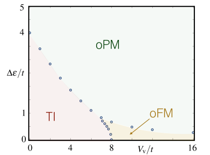
Figure 1: Phase diagram of the imbalanced Creutz-Hubbard ladder: Phase diagram displaying a topological insulator (TI) phase, and two other non-topological phases, namely an orbital phase with long-range ferromagnetic Ising order (oFM), and an orbital paramagnetic phase (oPM). The blue circles label numerical results, and the colored phase boundaries are a guide to the eye.

The presence of the energy imbalance breaks both time-reversal $U_{\mathsf{T}}h_{\rm C}(-k)^{*}U_{\mathsf{T}}^{\dagger}=+h_{\rm C}(q)$ and particle-hole $U_{\mathsf{C}}h_{\rm C}(-k)^{*}U_{\mathsf{C}}^{\dagger}=-h_{\rm C}(k)$ symmetries, since the term $(\textstyle\frac{1}{2}\Delta\varepsilon+2{t}_{\rm x}\sin k)$ in Eq. (33) is neither even, nor odd, under $k\leftrightarrow-k$. Hence, the above symmetries cannot be fulfilled for any unitary $U_{\mathsf{T}}$ or $U_{\mathsf{C}}$. On the other hand, there is a discrete sublattice symmetry $U_{\mathsf{S}}h_{\rm C}({k})U_{\mathsf{S}}^{\dagger}=-h_{\rm C}({k})$ with the operator $U_{\mathsf{S}}=\sigma_{y}$. Accordingly, the regime $\Delta\epsilon<4t$ with $\mathsf{W}_{1}=-1$ can be interpreted as a 1D AIII topological insulator creutz_hubbard ; GNW_model_spt .

The goal of this section is to study the fate of this topological phase in the presence of 4-Fermi terms

$$H_{\rm CH}=H_{\rm C}+\frac{V_{\rm v}}{2}\sum_{j}\sum_{\ell}c_{j,\ell}^{\dagger}\,c_{j,\bar{\ell}}^{\dagger}\,c_{j,\bar{\ell}}^{\phantom{\dagger}}\,c_{j,\ell}^{\phantom{\dagger}},$$ (36)

which can be understood as Hubbard density-density interactions (13) along the rungs of the ladder. In Ref. creutz_hubbard , we obtained a numerical estimate of the phase diagram for this Creutz-Hubbard model using Matrix-Product-State methods mps (see Fig. 1). In the present work, we will use these tools to benchmark the RG calculations, and test the validity of their connection to the topological Hamiltonian.

(b) Euclidean action and continuum QFT description.–

In this subsection, we present the Euclidean action for the continuum description of the Creutz-Hubbard ladder, which will be valid in the vicinity of the second-order quantum phase transition. We thus focus on the vicinity of $\Delta\epsilon=4t$, where the Wilson fermion at $k_{1}=-\pi/2$ becomes massless, while the one at $k_{0}=+\pi/2$ has a large positive mass. We note that setting $t=t_{\rm x}$ makes this mass very heavy $m_{0}=2$, such that the corresponding Wilson fermion lies already at the cutoff of the theory (i.e. maximum energy of the band). In any case, regardless of the particular value of $t/t_{\rm x}$, the fate of this fermion is to end in such a large mass limit as one approaches the IR limit of the RG transformations (i.e. the mass term is a relevant perturbation (25)). We thus believe that, without loss of generality, one can set $t=t_{\rm x}$ from the outset. Considering that this heavy fermion has a big positive mass, the topological invariant (35) is fully controlled by the mass of the lighter fermion around $k_{1}$, such that a non-trivial integer-valued Wilson loop is obtained provided that

$$\mathsf{W}_{1}={\rm e}^{{\rm i}2\pi\mathsf{CS}_{1}}=-1,\hskip 8.61108pt{\rm if}\hskip 4.30554pt{{\rm sgn}(m_{1})}=-1.$$ (37)

We start by reorganizing the action (15) for the Creutz-Hubbard Hamiltonian (36) in the regime $V_{\rm v}<\Delta\epsilon\approx 4t=4t_{\rm x}$ in a form that simplifies the RG calculations beyond tree level (25)-(26), namely $S_{\rm CH}=S_{0}+\delta S$ with

$$S_{0}=\bigintssss_{\{{k},\omega\}}\sum_{\eta={\rm R,L,u,d}}\overline{\psi}_{\eta}({k},\omega)(-{\rm i}\omega+\epsilon_{\eta}({k}))\psi_{\eta}^{\phantom{\dagger}}({k},\omega),$$ (38)

where we have introduced the flavor index $\eta$ to label the different Wilson fermions: (i) $\eta\in\{{\rm R,L}\}$ refers to the right- ($s_{\rm R}=1$) as and left-moving ($s_{\rm L}=-1$) modes around the Dirac point $k_{1}$, $\psi_{\eta}^{\phantom{\dagger}}({k},\omega)=(\psi_{1,\rm u}^{\phantom{\dagger}}({k},\omega)-s_{\eta}\psi_{1,\rm d}^{\phantom{\dagger}}({k},\omega)/\sqrt{2}$, which have energies $\epsilon_{\eta}({k})=s_{\eta}k$. The Wilson-mass term of the fermions around this point $m_{1}$, which is small for $\Delta\epsilon\approx 4t$, will be included in $\delta S$. In addition, (ii) we define the flavors $\eta\in\{{\rm u,d}\}$ for the positive- and negative-frequency modes around the point $k_{0}$, $\psi_{\eta}^{\phantom{\dagger}}({k},\omega)=\psi_{0,\eta}^{\phantom{\dagger}}({k},\omega)$, which have energies $\epsilon_{\eta}({k})=\pm m_{0}$. We note that the corrections to this heavy-mass limit (i.e. $\delta\epsilon_{\eta}({k})\approx\mp k^{2}$) can be included in $\delta S$. However, as occurred for the shorter-wavelength corrections (17), these perturbations are IR irrelevant already at tree level.

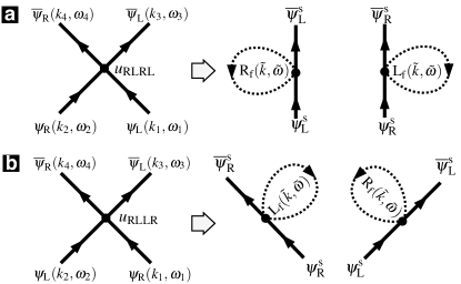
Figure 2: One-loop tadpole diagrams around $k_{1}$: (a) (left) Forward scattering of $(\eta_{1},\eta_{2})=({\rm L,R})$ fermions onto $(\eta_{3},\eta_{4})=({\rm L,R})$. (right) Tadpole diagrams by joining an incoming and outgoing line of the same $\eta\in\{\rm L,R\}$ flavor into a loop. The momentum inside the loop is constrained to a small region around the cutoff $\Lambda_{\rm c}/s\leq\tilde{k}\leq\Lambda_{\rm c}$. The loop integrals over the fast modes are labelled by $\eta_{\rm f}(\tilde{k},\tilde{\omega})$ and depicted by dashed closed lines. (b) (left) Backward scattering of $(\eta_{1},\eta_{2})=({\rm R,L})$ fermions onto $(\eta_{3},\eta_{4})=({\rm L,R})$. (right) Corresponding tadpole diagrams.

The perturbations that are relevant and marginal at tree level are contained in $\delta S=\delta S_{\rm m}+\delta S_{\rm int}$, where

$$\delta S_{\rm m}=\bigintssss_{\{{k},\omega\}}\sum_{\eta={\rm L,R}}m_{1}\Lambda_{\rm c}\overline{\psi}_{\eta}({k},\omega)\psi_{\bar{\eta}}^{\phantom{\dagger}}({k},\omega),$$ (39)

and we have introduced $\bar{\eta}={\rm L}$ ($\bar{\eta}={\rm R}$) for ${\eta}={\rm R}$ (${\eta}={\rm L}$). Clearly, the mass term mixes the right- and left-moving fermions around $k_{1}$, breaking explicitly the chiral symmetry of the free masless Dirac fermion (38) fradkin_book . The correction due to the Hubbard interaction (36), which must be normalized by the effective speed of light $c=2t_{\rm x}=2t$, can be expressed in a form similar to Eq. (19), namely

$$\delta S_{\rm int}=-\frac{1}{4}\bigintsss_{\{{k},\omega\}}\!\sum_{\{\bm{\eta}\}}u_{\bm{\eta}}\overline{\psi}_{\eta_{4}}(4)\overline{\psi}_{\eta_{3}}(3)\psi_{\eta_{2}}(2)\psi_{\eta_{1}}(1),$$ (40)

where we use similar conventions as below Eq. (19), and define $\sum_{\{\bm{\eta}\}}=\sum_{\eta_{1},\eta_{2},\eta_{3},\eta_{4}}$. These interaction terms describe the scattering between an incoming pair of fermions $(\eta_{1},\eta_{2})$ onto an outgoing pair $(\eta_{3},\eta_{4})$. Note that the dimensionless couplings $u_{\bm{\eta}}=u_{\eta_{4},\eta_{3},\eta_{2},\eta_{1}}$ should be antisymmetric with respect to $\eta_{4}\leftrightarrow\eta_{3}$, or $\eta_{2}\leftrightarrow\eta_{1}$, as a consequence of the anti-commuting nature of the Grassmann variables shankar_rg . Additionally, the particular form of the Hubbard interaction in Eq. (36) leads to couplings $u_{\bm{\eta}}$ without any momentum dependence.

In combination, these two features limit the possible scattering events underlying the action (40). For instance, for scattering processes that take place in the vicinity of a single point $k_{n}$, the only allowed couplings are $u_{\rm RLLR}:=V_{\rm v}/2t$, and $u_{\rm uddu}:=2V_{\rm v}/t$, together with all the possible permutations

$$\begin{split}u_{\rm RLLR}&=-u_{\rm LRLR}=-u_{\rm RLRL}=u_{\rm LRRL}:=V_{\rm v}/2t,\\ u_{\rm uddu}&=-u_{\rm udud}\,\,=\,\,-u_{\rm dudu}\,\,=\,\,u_{\rm duud}:=2V_{\rm v}/t,\\ \end{split}$$ (41)

All these scattering processes preserve the number of fermions with a given flavor $\eta$ (see the left panels of Figs. 2 (a) and (b) for the two possible scattering channels with an outgoing $(\eta_{3},\eta_{4})=(\rm L,R)$ pair).

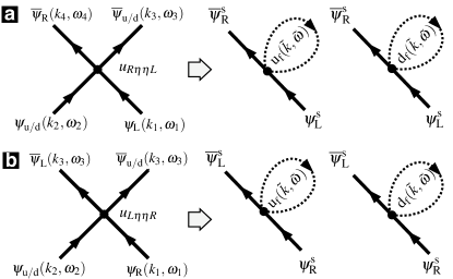
Figure 3: One-loop tadpole diagrams involving $k_{1}$ and $k_{0}$: (a) (left) Scattering of $(\eta_{1},\eta_{2})=({\rm L,u/d})$ fermions onto $(\eta_{3},\eta_{4})=({\rm u/d,R})$. (right) Tadpole corrections to the mass of the light fermions by joining an incoming and outgoing line of the heavy fermions (we use the same conventions as in Fig. 2) . (b) Same as for (a) but for the scattering of $(\eta_{1},\eta_{2})=({\rm R,u/d})$ fermions onto $(\eta_{3},\eta_{4})=({\rm u/d,L})$.

In addition, there will be scattering processes that involve fermions from both Dirac points $k_{0}$ and $k_{1}$, which can be organized in two sets. The first set consists of scattering processes that conserve the number of fermions around each point, but may change their flavor e.g. a $L\leftrightarrow R$ and $u\leftrightarrow d$, namely

$$\begin{split}u_{\rm RuuR}&=-u_{\rm RuuL}=-u_{\rm LuuR}=u_{\rm LuuL}:=V_{\rm v}/4t,\\ u_{\rm RddR}&=\phantom{-}u_{\rm RddL}=\phantom{-}u_{\rm LddR}=u_{\rm LddL}:=V_{\rm v}/4t,\\ u_{\rm LudL}&=-u_{\rm RudR}=-u_{\rm RudL}=u_{\rm LudR}:=V_{\rm v}/4t,\\ u_{\rm LduL}&=-u_{\rm RduR}=-u_{\rm LduR}=u_{\rm RduL}:=V_{\rm v}/4t,\\ \end{split}$$ (42)

plus all permutations $\eta_{1}\eta_{2}$, $\eta_{3}\eta_{4}$ with their relative signs. The second set corresponds to the so-called Umklapp scattering, i.e. processes where the number of fermions around each point changes in pairs

$$\begin{split}u_{\rm udRL}&=-u_{\rm udLR}=-u_{\rm duRL}=u_{\rm duLR}:=V_{\rm v}/t,\\ u_{\rm LRdu}&=-u_{\rm LRud}=-u_{\rm RLud}=u_{\rm RLud}:=V_{\rm v}/t.\\ \end{split}$$ (43)

We note that momentum conservation can still be achieved up to a reciprocal lattice vector $\pm 2(k_{1}-k_{0})=\pm 2\pi$.

Equations (38)-(40) set the stage for the RG study of correlation effects in the one-dimensional AIII topological insulator beyond tree level. As discussed in detail below, in the vicinity of $\Delta\epsilon=4t=4t_{\rm x}$, we shall use these corrections to predict the critical line separating topological and normal insulating phases at finite repulsive interactions $V_{\rm v}>0$.

III.2 Loop-expansion: running of the Wilson masses and topological invariants in presence of interactions

In this subsection, we consider the first- and second-order terms of the cumulant expansion (24) of the quartic interactions (40), focussing on its effects on the renormalization of the Wilson masses and the topological invariant. This will allow us to determine the critical line that connects to the non-interacting RG fixed point separating the topological and trivial insulators, and to show that such a critical line delimits the region of the phase diagram where the ground-state corresponds to a correlated topological insulator.

(a) Vanishing tadpoles considering light Wilson fermions.–

In the regime $\Delta\epsilon\approx 4t=4t_{\rm x}$, the Wilson masses fulfil $|m_{1}|\ll|m_{0}|$, and one may expect that the heavy fermions around $k_{0}$ shall not have any influence on the lighter fermions around $k_{1}$, which in turn determine the onset of a topological phase (i.e. the mass-inversion point $m_{1}<0$). Following this line of reasoning, to see how this Wilson mass runs with the cutoff $m_{1}(\Lambda_{\rm c})$, and determine how the RG fixed point ${m_{1}}=0$ changes with interactions, it would suffice to consider scattering events (40) in the vicinity of $k_{1}$, i.e. scattering between left- and right-moving modes described by the first line of Eq. (41). The first-cumulant correction to the coarse-grained action would then arise from the following terms

$$\begin{split}\langle\delta S^{k_{1}}_{\rm int}\rangle_{\rm f}=&\frac{1}{4}\bigintsss_{\{{k},\omega\}}\!\sum_{{\eta}={\rm L,R}}u_{\eta\bar{\eta}\bar{\eta}\eta}\left(\left\langle\overline{\psi}_{\bar{\eta}}^{\rm f}(3)\psi_{\bar{\eta}}^{\rm f}(2)\right\rangle_{\rm f}\overline{\psi}_{\eta}^{\rm s}(4)\psi_{\eta}^{\rm s}(1)+\left\langle\overline{\psi}_{{\eta}}^{\rm f}(4)\psi_{{\eta}}^{\rm f}(1)\right\rangle_{\rm f}\overline{\psi}_{\bar{\eta}}^{\rm s}(3)\psi_{\bar{\eta}}^{\rm s}(2)\right)\\ +&\frac{1}{4}\bigintsss_{\{{k},\omega\}}\!\sum_{{\eta}={\rm L,R}}u_{\eta\bar{\eta}{\eta}\bar{\eta}}\left(\left\langle\overline{\psi}_{\bar{\eta}}^{\rm f}(3)\psi_{\bar{\eta}}^{\rm f}(1)\right\rangle_{\rm f}\overline{\psi}_{\eta}^{\rm s}(4)\psi_{\eta}^{\rm s}(2)+\left\langle\overline{\psi}_{{\eta}}^{\rm f}(4)\psi_{{\eta}}^{\rm f}(2)\right\rangle_{\rm f}\overline{\psi}_{\bar{\eta}}^{\rm s}(3)\psi_{\bar{\eta}}^{\rm s}(1)\right),\\ \end{split}$$ (44)

where $\langle\overline{\psi}_{{\eta}}^{\rm f}(j)\psi_{{\eta}}^{\rm f}(j^{\prime})\rangle_{\rm f}=\delta(\omega_{j}-\omega_{j^{\prime}})\delta(k-{k^{\prime}})/({\rm i}\omega_{j}-\epsilon_{\eta}(k))$ is obtained from the free-fermion propagator (21) by working on the corresponding eigenbasis of the non-interacting single-particle Hamiltonian.

These contributions can be depicted in terms of the so-called tadpole diagrams (see the right panels of Figs. 2 (a) and (b) for $\eta={\rm L}$), which include a single closed loop over the fast modes. It is already apparent from the fast-mode loops of these figures, without any further calculation, that these terms can only contribute with $\langle\delta S^{k_{1}}_{\rm int}\rangle_{\rm f}\propto(\overline{\psi}_{\rm R}^{\rm s}(k,\omega)\psi_{\rm R}^{\rm s}(k,\omega)+\overline{\psi}_{\rm L}^{\rm s}(k,\omega)\psi_{\rm L}^{\rm s}(k,\omega))$, which is an irrelevant common shift of the on-sites energies for the slow modes. However, there is no one-loop term that yields a correction to the mass term mixing the different fermion chiralities $\langle\delta S^{k_{1}}_{\rm int}\rangle_{\rm f}\propto(\overline{\psi}_{\rm R}^{\rm s}(k,\omega)\psi_{\rm L}^{\rm s}(k,\omega)+\overline{\psi}_{\rm L}^{\rm s}(k,\omega)\psi_{\rm R}^{\rm s}(k,\omega))$, inducing thus a non-vanishing mass (39) around $k_{1}$. This result is in contradiction to the numerical data displayed in Fig. 1, where the non-interacting critical point at $\Delta\epsilon=4t$ flows towards smaller values of the imbalance linearly $(\Delta\epsilon-4t)\propto-V_{\rm v}$, for $V_{\rm v}\ll\Delta\epsilon$. Accordingly, the Wilson mass corresponding to this fixed point $m_{1}$ should get a renormalization $\tilde{m}_{1}=m_{1}+\delta m_{1}(V_{\rm v})$ (27) linear in the interaction strength $\delta m_{1}(V_{\rm v})\propto V_{\rm v}$. We can thus conclude that, when restricting to the slow modes of the continuum description, it is not possible to obtain non-zero tadpole corrections that can account for the numerical phase diagram.

We note, at this point, that 4-Fermi continuum QFTs can display the phenomenon of dynamical mass generation, where an interacting massless Dirac fermion acquires a mass that spontaneously breaks chiral symmetry GN_model . The scaling of the dynamically-generated mass with the interaction strength is, however, non-perturbative GN_model ; GNW_model_spt , and cannot account for the aforementioned linear dependence. We will extend on the interplay of lattice effects and a dynamically-generated mass in the last section with our conclusions and outlook.

(b) Tadpoles considering also heavy Wilson fermions.–

Let us now explore how a linear running of the Wilson mass can be obtained by considering the effect that the heavy fermion around $k_{0}$ may have on the lighter mass $m_{1}$ of the fermion around $k_{1}$. The heavy fermion around $k_{0}$, lying at the cutoff of the theory, may indeed renormalize the parameters of the QFT when integrated out during the RG coarse-graining. Inspecting Eqs. (42)-(43), one realizes that the couplings $u_{\rm LuuR},u_{\rm RuuL},u_{\rm LddR},u_{\rm RddL}$, together with their corresponding permutations, can lead to tadpole diagrams that indeed induce a correction to the mass (see Fig. 3). The first-cumulant contribution to the coarse-grained action yields

$$\begin{split}\langle\delta S^{k_{1}k_{0}}_{\rm int}\rangle_{\rm f}=&\frac{1}{4}\bigintsss_{\{{k},\omega\}}\!\sum_{{\eta}={\rm u,d}}4\left(u_{\rm R{\eta}{\eta}L}\left\langle\overline{\psi}_{\eta}^{\rm f}(4)\psi_{{\eta}}^{\rm f}(1)\right\rangle_{\!\!\rm f}\overline{\psi}_{\rm R}^{\rm s}(3)\psi_{\rm L}^{\rm s}(2)+u_{\rm L{\eta}{\eta}R}\left\langle\overline{\psi}_{\eta}^{\rm f}(4)\psi_{{\eta}}^{\rm f}(1)\right\rangle_{\!\!\rm f}\overline{\psi}_{\rm L}^{\rm s}(3)\psi_{\rm R}^{\rm s}(2)\right),\\ \end{split}$$ (45)

where the additional factor of $4$ comes from considering the contribution of all possible permutations, e.g. $u_{\rm LuuR}=-u_{\rm uLuR}=-u_{\rm LuRu}=u_{\rm uLRu}$, all of which contribute equally.

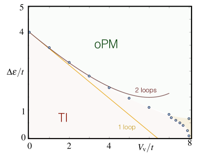
Figure 4: Benchmark of the RG prediction for the critical line: Comparison of the one-loop (49) (yellow line) and two-loop (52) (red line) predictions of the critical line. The blue circles label numerical results of Fig. 1 in the region of weak to moderate interactions.

If we now perform the loop integrals, we obtain $\int_{\mathbb{R}}\!\!\frac{{\rm d}\omega_{4}}{2\pi}\!\int_{\frac{\Lambda_{\rm c}}{s}}^{\Lambda_{\rm c}}\!\!\frac{{\rm d}k_{4}}{(2\pi)}\int_{\mathbb{R}}\!\!\frac{{\rm d}\omega_{1}}{2\pi}\int_{\frac{{\Lambda_{\rm c}}}{s}}^{\Lambda_{\rm c}}\!\!\frac{{\rm d}k_{1}}{(2\pi)}\left\langle\overline{\psi}_{\eta}^{\rm f}(4)\psi_{{\eta}}^{\rm f}(1)\right\rangle_{\rm f}=\mp\frac{\Lambda_{\rm c}}{\pi}(1-\frac{1}{s})$ for $\eta={\rm u,d}$, respectively. To compare with the original action, we must now rescale the momentum and frequency (22) to reset the original cutoff. Accordingly, the slow modes should also be transformed

$$\begin{split}\psi^{\rm s}_{\rm R/L}({k},\omega)\to{\psi}^{\prime}_{\rm R/L}({k}^{\prime},\omega^{\prime})=s^{-(d+2)/2}{\psi}^{\rm s}_{\rm R/L}({k}^{\prime}/s,\omega^{\prime}/s),\end{split}$$ (46)

such that the first-order cumulant (45) contributes with a correction to the Wilson mass (39), namely

$$\langle\delta S^{k_{1}k_{0}}_{\rm int}\rangle_{\rm f}=\bigintssss_{{k},\omega}\sum_{\eta={\rm L,R}}\delta m_{1}^{(1)}\Lambda_{{\rm c}}\overline{\psi}_{\eta}({k},\omega)\psi_{\bar{\eta}}^{\phantom{\dagger}}({k},\omega).$$ (47)

Here, we have introduced the Wilson mass shift to one loop $\delta m_{1}^{(1)}$, which modifies the $\beta_{m_{1}}$ function in the following way

$$\delta m_{1}^{(1)}=\frac{V_{\rm v}}{2\pi t}(s-1),\hskip 12.91663pt\beta_{m_{1}}=\frac{{\rm d}m_{1}}{{\rm d}\log s}=m_{1}+\delta\beta_{m_{1}}^{(1)}.$$ (48)

The RG fixed point is then determined by the bare lattice parameters that lead to a vanishing $\beta_{m_{1}}$ function, namely

$$\frac{\Delta\epsilon}{4t}-1=-\frac{V_{\rm v}}{2\pi t}\implies\left.\frac{\Delta\epsilon}{t}\right|_{\rm c}=4-\frac{2}{\pi}\frac{V_{\rm v}}{t}.$$ (49)

The comparison of this prediction with the numerical results shows a good agreement in the regime of weak interactions (see the yellow line in Fig. 4). We note that this one-loop correction to the mass agrees exactly with a self-consistent mean-field treatment that relies on the mapping of the Creutz-Hubbard model to a pair of coupled quantum Ising models creutz_hubbard . The advantage of the present RG approach is that, on the hand, it can be improved systematically by considering higher orders in the cumulant expansion. On the other hand, as discussed below, we can not only predict the position of the critical line, but also show that the region it delimits corresponds to a correlated $\mathsf{AIII}$ topological insulator.

(c) Two-loop corrections to the light Wilson mass.–

Let us now move on to the second-order cumulant contributions (24) to the coarse-grained action, which will yield two-loop corrections to the Wilson mass that can be accounted for by considering the so-called one-particle irreducible Feynman diagrams with two interaction vertices and two external lines with right- and left-moving fermions.

In analogy to the discussion below Eq. (44), we note that it is not possible to obtain two-loop corrections to the mass by simply focusing on the light fermion around $k_{1}$ (i.e. scattering events in first line of Eq. (41)). By incorporating the interactions with the heavy fermion around $k_{0}$, we can have the contributions to the Wilson mass depicted in Fig. 5, where we recall that the closed loops are formed by heavy-fermion propagators. In contrast to the standard situation in other interacting QFTs amit_book , where the double tadpole of Fig. 5 (a) would contribute to the mass, here we find that only the “saturn diagram” of Fig. 5 (b) does contribute with a second-order shift of the mass

$$\left\langle\left(\delta S^{K_{1}K_{0}}_{\rm int}\right)^{2}\right\rangle_{\!\!\rm c,f}\!=\bigintssss_{{k},\omega}\sum_{\eta={\rm L,R}}\delta{m}^{(2)}_{1}\Lambda_{{\rm c}}\overline{\psi}_{\eta}({k},\omega)\psi_{\bar{\eta}}^{\phantom{\dagger}}({k},\omega).$$ (50)

Here, we have introduced the two-loop mass shift

$$\delta{m}_{1}^{(2)}=-\frac{3}{8\pi^{2}}\frac{V_{\rm v}^{2}}{m_{0}t^{2}}(s-1),\hskip 12.91663pt\beta_{m_{1}}=m_{1}+\delta\beta_{m_{1}}^{(1)}+\delta\beta_{{m}_{1}}^{(2)}.$$ (51)

which should be evaluated for the mass of the heavy fermions $m_{0}=\Delta\epsilon/4t+1$ at the bare lattice parameters that yield the RG fixed point with first-order corrections (49), such that $m_{0}=2-V_{\rm v}/2\pi t$. Hence, the critical line of the model with two-loop corrections follows from the condition of a vanishing $\beta_{m_{1}}$ function, and yields

$$\left.\frac{\Delta\epsilon}{t}\right|_{\rm c}=4-2\left(\frac{V_{\rm v}}{\pi t}\right)+\frac{3}{4}\left(\frac{V_{\rm v}}{\pi t}\right)^{2}\frac{1}{4-\left(\frac{V_{\rm v}}{\pi t}\right)}.$$ (52)

The comparison of this prediction with the numerical results shows a much better agreement in the regime of weak to intermediate interactions (see the red line of Fig. 4).

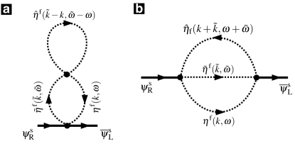
Figure 5: Two-loop diagrams for the Wilson mass term: (a)-(b) Possible two-loop diagrams for the correction to the mass of the light fermions $\eta_{j}\in\{\rm L,R\}$ by virtual creation-annihilation of light/heavy fermions in fast modes $\eta,\tilde{\eta},\hat{\eta}\in\{\rm R,L,u,d\}$.

(d) RG flows and the effective topological Hamiltonian.–

Let us now consider the nature of the two phases separated by this critical line from the perspective of the topological Hamiltonian (29). As discussed below Eq. (29), the renormalization of the Wilson masses (27) contributes to the zero-frequency self-energy in a very simple manner, which allows to diagonalize the topological Hamiltonian (29) in complete analogy to the single-particle one. In the present case, the topological Hamiltonian can be expressed as

$$h_{\rm top}({k})=-2t\sigma^{x}\cos k+\left(\textstyle\frac{1}{2}\Delta\tilde{\epsilon}+2t\sin k\right)\sigma^{z},$$ (53)

where the previous two-loop corrections contribute to

$$\Delta\tilde{\epsilon}=\Delta\epsilon+\frac{2}{\pi}V_{\rm v}-\frac{3V_{\rm v}}{4\pi^{2}t}\left(4-\frac{V_{\rm v}}{\pi t}\right).$$ (54)

The calculation of the topological invariants now directly yields Eq. (31), and we obtain a non-zero topological invariant for the correlated topological insulator when

$$\mathsf{W}_{1}={\rm e}^{{\rm i}2\pi\mathsf{CS}_{1}}=-1,\hskip 8.61108pt{\rm if}\hskip 4.30554pt{{\rm sgn}(\tilde{m}_{1})}=-1.$$ (55)

Since we know the two-loop corrections to the mass, we can characterize the nature of the insulating phases separated by the critical line: (i) for $\frac{\Delta\epsilon}{t}>\left.\frac{\Delta\epsilon}{t}\right|_{\rm c}$ (i.e. above the critical line), the mass $\tilde{m}_{1}>0$, such that $\mathsf{CS}_{1}=0$, and the Wilson loop is trivial $\mathsf{W}_{1}=1$. Accordingly, the ground-state corresponds to a normal band insulator. (ii) for $\frac{\Delta\epsilon}{t}<\left.\frac{\Delta\epsilon}{t}\right|_{\rm c}$ (i.e. below the critical line), the mass $\tilde{m}_{1}<0$, such that $\mathsf{CS}_{1}=\textstyle\frac{1}{2}$, and the Wilson loop is $\mathsf{W}_{1}=-1$. Accordingly, the ground-state corresponds to a topological $\mathsf{AIII}$ insulator. This behaviour is in complete agreement with Fig. 1, and thus can serve as a quantitative test of the validity of the RG picture of correlated topological insulators presented in this work.

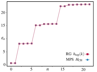
Figure 6: Entanglement spectrum of the Creutz-Hubbard ladder: Lowest $N_{\rm ES}=22$ eigenvalues of the entanglement spectrum $\epsilon_{n}\in{\rm ES}(\rho_{\ell})$ for the Creutz-Hubbard ladder (36) for $\Delta\epsilon=2.2t$, $V_{\rm v}=0.2t$, which lies inside the TI region of Fig. 4. We compare the results obtained via the MPS numerical simulations (squares), and via the RG-corrected topological Hamiltonian (circles)  (53).

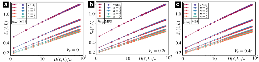
Figure 7: Entanglement entropies of the critical Creutz-Hubbard ladder: Von Neumann and Rényi block entanglement entropies are represented as a function of the block chord length. The Hubbard interaction strengths are set to (a) $V_{\rm v}=0$, (b) $V_{\rm v}=0.2t$, and (c) $V_{\rm v}=0.4t$, while the corresponding energy imbalance $\Delta\epsilon$ is set to the critical value of Eq. (52) predicted by the RG calculations.

III.3 Entanglement spectroscopy: symmetry-protected topological phases and critical Luttinger liquids

In this subsection, we shall explore additional features of the zero-temperature Creutz-Hubbard ladder to benchmark the RG-corrected topological Hamiltonian (33). These features will become manifest in the bipartite correlations of a ground-state partitioned into two blocks of length $\ell$ and $L-\ell$, where $L=Na$ is the length of the whole ladder. In particular, we shall be interested in two types of correlations: entanglement entropies, and bi-partite fluctuations. The former are related to the so-called entanglement spectrum, which serves to characterize the topological properties of an interacting topological insulator as a symmetry-protected topological (SPT) phase. The latter will be used to characterize the critical line delimiting the topological-insulating region in more detail.

(a) SPT entanglement and the topological Hamiltonian.–

Let us start by focusing on the entanglement of the ground-state, which can defined via the block reduced density matrices $\rho_{\ell}={\rm Tr}_{L-\ell}\{|\epsilon_{\rm gs}\rangle\langle\epsilon_{\rm gs}|\}$. Among the various existing measures of entanglement on a bi-partite scenario entanglement_measures , the entanglement entropies (EEs) enjoy a privileged status within the realm of quantum many-body systems ent_many_body ; EE_many_body . In particular, the so-called Rényi EEs are defined for all $n>0$

$$S_{n}(\ell,L)=\frac{1}{1-n}\log\big{(}{\rm Tr}\left\{\left(\rho_{\ell}\right)^{n}\right\}\big{)},$$ (56)

and include the Von Neuman entanglement entropy (VNEE) $S(\ell,L)=-{\rm Tr}\{\rho_{\ell}\log(\rho_{\ell})\}=\lim_{n\to 1}S_{n}(\ell,L)$ as a limiting case. Moreover, the Rényi EEs are related to the moments of the reduced density matrix moments_es , and can be used to construct the full entanglement spectrum  entanglement_spectrum , which is defined by the set of all eigenvalues ${\rm ES}(\rho_{\ell})=\sigma(H_{\rm E})$ of the entanglement Hamiltonian $H_{\rm E}$, obtained by expressing the reduced density matrix as an equilibrium Gibbs state $\rho_{\ell}\propto{\rm e}^{-H_{\rm E}}$.

For non-interacting systems, $H_{\rm E}$ has a closed-form expression as a quadratic operator that can be derived exactly from the exact diagonalization of the original Hamiltonian red_density_matrices_free . For interacting systems, the entanglement spectrum $\epsilon_{n}\in{\rm ES}(\rho_{\ell})$ can be obtained approximately by the MPS simulations mps , which give direct access to the Schmidt values $\lambda_{n}$ of the bipartition, such that $\epsilon_{n}=-2\log\lambda_{n}$. As shown in ES_spt , the entanglement spectrum can be used to characterize SPT phases such as correlated topological insulators, as it displays an exact degeneracy related to the existence of many-body edge modes  ES_spt . In Fig. 6, we show how this feature is fulfilled clearly for the correlated $\mathsf{AIII}$ topological insulator (36). As a comparison, we display the entanglement spectrum of the full Creutz-Hubbard ladder (36), and that of the RG-corrected topological Hamiltonian (33), which can be calculated exactly via the two-point correlation functions peschel_rho_red_corr . Both methods display the aforementioned degeneracies for the correlated topological insulator (55), and show a clear quantitative agreement providing an additional test of the validity of the RG-corrected topological Hamiltonian approach.

It is also worth mentioning that our predictions can be provided experimentally. In  dalmonte_papers the authors proposed an immediate, scalable recipe for implementation of the entanglement Hamiltonian, and measurement of the corresponding entanglement spectrum as spectroscopy of the Bisognano-Wichmann Hamiltonian  bisignano_paper with synthetic quantum systems.

(b) Bi-partite fluctuations and the Luttinger parameter.–

We now explore the scaling region of the quantum phase transition between the topological and trivial band insulators (see Fig. 4) from the perspective of bi-partite correlations. In Fig. 7, we represent the critical Rényi EEs (56) obtained by the two approaches as a function of the so-called chord length $D(\ell,L)=(2L/\pi)\sin(\pi\ell/L)$. As can be observed in this figure, the agreement between effective RG model and full one, is very good for weak interactions, but small deviations become apparent in the higher-order Rényi EEs as the Hubbard interactions increase and we move along the critical line of Fig. 4.

We would like to understand the origin of these small differences. On the one hand, they might simply be caused by inaccuracies in the RG-corrected imbalance (54). However, for the range of Hubbard interactions hereby explored, we have found that the differences in the critical points are vanishingly small. On the other hand, they might be caused by the approximations inherent to the topological Hamiltonian (29), namely considering only the static part of the self-energy to define an effective single-particle Hamiltonian. In the present context, the critical properties of the topological Hamiltonian (33) are always governed by a single massless Dirac fermion, which might not be an accurate description of the scaling region of the full Creutz-Hubbard ladder as one moves along the critical line by increasing the interactions.

In order to explore this question further, we will explore the particular scaling of the critical bi-partite correlations with the chord distance. Due to non-extensive nature of the EEs $S_{n}(\ell,L)=S_{n}(L-\ell,L)$, the bipartite correlations might be expected to be contained within the boundary of the bipartition, which leads to the so-called entropic logarithmic area laws area_law_rmp . As occurs for the VNEE vn_entropy , the Rényi EEs also display area-law violations for one-dimensional critical systems cft_entropy , which contain information about the underlying conformal field theory (CFT) that describes the long-wavelength properties of the system cft_book . For open boundary conditions, one finds that the Rényi EEs can be expressed as

$$S_{n}(\ell,L)=S_{n}^{\rm CFT}(\ell,L)+\delta S_{n}(\ell,L),$$ (57)

which contains a logarithmic violation of the area law that depends on the central charge $c$ of the CFT

$$S_{n}^{\rm CFT}(\ell,L)=\frac{c}{12}\left(1+\frac{1}{n}\right)\log D(\ell,L),$$ (58)

together with a non-universal correction $\delta S_{n}(\ell,L)$. We note that the logarithmic scaling of these EEs for various interactions displayed in Fig. 7 is consistent with a central charge $c\approx 1$, which corresponds to the CFT of a free compactified boson cft_book . This agrees with the leading-order scaling of the Rényi EEs for the topological Hamiltonian (33), such that the aforementioned deviations must be contained in the non-universal terms $\delta S_{n}(\ell,L)$. In particular, one possibility is that the Luttinger parameter, which is always fixed to $K=1$ for the RG-corrected topological Hamiltonian (33), becomes $K\neq 1$ for the full Creutz-Hubbard ladder (36).

As first realized for the Von Neumann EE with open boundary conditions ee_corrections_luttinger , the non-universal corrections to the Rényi EEs renyis_corrections for systems whose critical behavior is described by the free-boson CFT (i.e. Luttinger liquids lutt_liq ) find the following closed-form expression

$$\delta S_{n}(\ell,L)=F_{n}\left(\frac{\ell}{L}\right)\frac{\cos(2k_{\rm F}\ell+\omega)}{\big{(}2\sin(k_{\rm F})D(\ell,L)\big{)}^{K/n}},$$ (59)

where $k_{\rm F}$ is Fermi’s momentum, $K$ is the so-called Luttinger parameter, $F_{n}(\ell/L)$ is a scaling function, and $\omega$ is a constant phase-shift that controls the oscillating nature of the corrections. For instance, for spin-$\textstyle\frac{1}{2}$ Heisenberg-type Luttinger liquids (i.e. XXZ model), where $k_{\rm F}=\pi/2$, one finds $\omega=0$ such that the correlations display a characteristic alternating behavior ee_corrections_luttinger ; renyis_corrections . On the other hand, for hard-core bosons with dipolar interactions at quarter filling, where $k_{\rm F}=\pi/4$, one needs to set $\omega\approx\pi/2$ to capture the oscillations REE_K_dipolar_boson .

We note that this characteristic oscillatory behavior is in principle useful to extract numerically the corresponding Luttinger parameter taddia_thesis . Unfortunately, for the Creutz-Hubbard ladder, we have found that these oscillations are absent, such that the fitting procedure to extract the Luttinger parameter is not sufficiently accurate. We now provide an alternative route to extract the Luttinger parameter by exploring the quantum noise in models with a conserved quantity, such as the total fermion number $N=\sum_{j}\big{(}c_{j,{\rm u}}^{\dagger}c_{j,{\rm u}}^{\phantom{\dagger}}+c_{j,{\rm d}}^{\dagger}c_{j,{\rm d}}^{\phantom{\dagger}}\big{)}$ in the Creutz-Hubbard ladder (36). As first realized in fluctuations_entropy , noise in certain quantum-transport scenarios can be directly related to entropic entanglement measures. In fact, for free-fermion systems noise_cumulants_entropy_free_fermions , it can be shown rigorously that any Rényi EE (56) can be reconstructed from the knowledge of the noise cumulants for a certain bi-partition of the system. In free-fermion systems where the noise is purely Gaussian, it suffices to consider the second cumulant (i.e. variance) of the conserved quantity restricted to the bi-partition $N_{\ell}$, which is sometimes referred to as the bi-partite fluctuations

$$S^{\rm free}_{n}(\ell,L)=\frac{\pi^{2}}{12}\!\left(1+\frac{1}{n}\right)\!\mathcal{F}(\ell,L),\hskip 6.45831pt\mathcal{F}(\ell,L)=\langle(N_{\ell}-\langle N_{\ell}\rangle)^{2}\rangle.$$ (60)

In the case of models that can be mapped onto the free-boson $c=1$ CFT (i.e. Luttinger liquids), a similar expression holds as fluctuations are Gaussian noise_cumulants_lutt . The difference is that the Luttinger parameter also appears in the proportionality

$$S^{\rm CFT}_{n}(\ell,L)=\frac{\pi^{2}}{12K}\left(1+\frac{1}{n}\right)\mathcal{F}(\ell,L).$$ (61)

Using the expression of the CFT prediction for the Renyi-entropy (58), one finds that the bi-partite fluctuations of a Luttinger liquid with conserved particle number should scale with the chord distance as follows

$$\mathcal{F}(\ell,L)=\frac{K}{\pi^{2}}\log(D(\ell,L)).$$ (62)

Accordingly, the bi-partite fluctuations of a critical Luttinger liquid also show an area-law violation, and one can use them to extract the underlying Luttinger parameter $K$. We note that this additional conservation law could also be combined with the entanglement entropies, leading to an equipartion that may allow for more accurate extractions of the $K$ parameter sierra_paper .

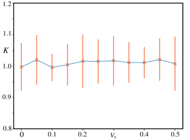
Figure 8: Luttinger parameter at criticality: The Luttinger parameter $K$ is extracted by fitting the bi-partite fluctuations $\mathcal{F}(\ell,L)$ obtained by the MPS numerical simulations to the linear logarithmic scaling with the chord length of Eq. (62). For each critical point $(\Delta\epsilon,V_{\rm v})$, we extract the thermodynamic value of the Luttinger parameter by extracting the corresponding $K_{L}$ values for various lengths $L/a\in[64,192]$, and fitting them to $K_{L}=K+c_{1}/L+c_{2}/L^{2}$.

In Fig. 8, we represent the Luttinger parameter $K$ for the critical Creutz-Hubbard ladder in the thermodynamic limit. We modify the Hubbard interaction strengths $V_{\rm v}$, and fix the energy imbalance $\Delta\epsilon$ to the RG-predicted value $\Delta\epsilon_{\rm c}$ of Eq. (52), such that the system lies at the critical line. The bi-partite fluctuations $\mathcal{F}(\ell,L)$ are numerically calculated using our MPS algorithm, and the value of $K$ is extracted following the procedure detailed in the corresponding caption. As this figure shows, the Luttinger parameter remains very close to the value $K\approx 1$, which would correspond to a free massless Dirac fermion as the CFT controlling the critical scaling. Let us note, however, that this numerical procedure has turned out to be very sensitive to small variations of the parameters. The error bars displayed in Fig. 8 correspond to the Luttinger parameter obtained by modifying the energy imbalance within $(\Delta\epsilon_{\rm c}-0.01t,\Delta\epsilon_{\rm c}+0.01t)$ for 10 different values of $\Delta\epsilon$, and obtaining the standard deviation of all the corresponding Luttinger parameters $K$. Accordingly, although it seems that the Luttinger parameter remains at $K\approx 1$ as the interactions are increased, our numerical results are not conclusive, as minor modifications in $\Delta\epsilon$ can lead to large variations in $K$. In case $K=1$ all along the critical line, the aforementioned differences might be caused by further non-universal and finite-size corrections. However, we note again that due to the sensitivity found in this problem, further numerical analysis shall be required in the future to clarify this point.

IV Conclusions and Outlook

In this work, we have presented a detailed study of the use of the RG to obtain an effective relativistic QFT that provides a continuum long-wavelength description of correlated topological insulators. Our description is valid for a variety of minimal models that serve as representatives of various topological insulators Bernevig , and are related to self-interacting fermionic lattice field theories in various dimensions lattice_book , which we refer to as topological Wilson-Hubbard matter.

We have shown that a Wilsonian RG, where the effect of integrating high-energy modes as the cutoff is reduced to focus on long-wavelength phenomena leads to a renormalization of the microscopic couplings, provides a neat description of these correlated topological insulators. At the so-called tree level, and generic to various dimensions, the RG approach offers a neat qualitative connection between the topological invariants in the long-wavelength limit and the flat-band limit of topological insulators. This connection becomes quantitative by using the RG flows of the parameters in connection to the so-called topological Hamiltonian, which includes static self-energy corrections to characterize the many-body topological invariant of the correlated topological insulator.

Going beyond tree level, we have shown that a loop expansion of the Wilsonian RG offers a quantitative route to understand the topological phase transitions that occur in Wilson-Hubbard matter, separating the correlated topological insulator from other non-topological phases. We have benchmarked the two-loop RG predictions for a particular 1D model, the imbalanced Creutz-Hubbard ladder, to quasi-exact numerical simulations based on matrix product states. This numerical comparison shows a very good agreement in the determination of the critical line determining the topological quantum phase transition, as well as various bi-partite correlations of the topological phase and the critical line. This benchmark may motivate the extension of the RG calculations to higher-dimensional correlated topological insulators in the future.

Let us now comment on the interpretation of our results from the perspective of dynamical mass generation in QFTs. As advanced in the main text, 4-Fermi continuum QFTs can display chiral symmetry breaking via dynamical mass generation GN_model . However, the scaling of the dynamically-generated mass with the 4-Fermi interaction strength is non-perturbative, which differs from the numerical matrix-product-state simulations for the particular lattice model studied in this work. Therefore, we believe that it is not possible to capture the physics of this type of correlated topological insulators by a continuum QFT if one insists on disregarding the heavy Wilson fermions lying at the cutoff of the lattice field theory, and considers only the 4-Fermi continuum QFTs for the light Wilson fermions. Our RG calculations indicate that the role of these heavy fermions in the RG flows of Wilson-Hubbard topological matter is very important.

In this context, the mapping of the imbalanced Creutz-Hubbard ladder GNW_model_spt , and other 1D correlated topological insulators kuno_SSH_int , to discretized Gross-Neveu lattice field theories offers a more concrete perspective on such a dynamical mass generation. Large-$N$ calculations show that, on top of the dynamically-generated mass generation GN_model , there are additive renormalizations of the mass when one considers the complete lattice action GNW_model_spt ; kuno_SSH_int . From the perspective of the continuum limit and our RG calculations, it seems to us that the interplay of light and heavy Wilson fermions in the RG flows is actually capturing this additive mass renormalization, and the two-loop calculations allow us to go beyond the $N\to\infty$ predictions for weak interactions GNW_model_spt ; kuno_SSH_int . It would be very interesting to explore this connection further, and see if both approaches can even be combined to provide a more accurate description of the topological phase transition, especially in higher dimensions.

Let us finally also comment on recent efforts to formulate a different RG for correlated topological insulators, which offers a very interesting alternative to the standard Wilsonian scheme rg_correlated_top_insulators . In this approach, one can build a scaling theory from the fact that the topological curvature, e.g. Berry connection, associated to the topological invariant presents some divergence at a topological quantum phase transition. Instead of changing the cutoff and integrating fast modes a la Wilson, this approach obtains RG flows by studying how this curvature changes with a flow of the microscopic parameters around high-symmetry points in momentum space curvature_rg . It would be very interesting to compare the predictions of this so-called curvature renormalization group (CRG) to our more-standard Wilsonian RG, in particular in the context of the imbalanced Creutz-Hubbard ladder, where the quasi-exact numerical results allow for a very detailed benchmark.

Finally, let us comment on one of the points raised in the introduction, namely the possibility of using condensed-matter analogues to explore models of high-energy physics. Besides the solid-state materials mentioned, ultracold gases of neutral atoms trapped in periodic light potentials cold_atom_review have become a very-flexible platform to explore a variety of analogues that can be described accurately by the particular model under study, acting as quantum simulators q_sim_review_1 . We note that the Wilson-Hubbard topological matter described in this work may find experimental realizations along the lines of wilson_atoms ; GNW_model_spt ; kuno_SSH_int ; wilson_hauke ; wilson_kuno ; KHS18 in the field of cold atoms.

References

- (1) L. Landau, Zh. Eksp. Teor. Fiz. 7, 19 (1937) [Phys. Z. Sowjetunion 11, 26 (1937)].
- (2) V. Ginzburg and L. Landau, Zh. Eksp. Teor. Fiz. 20 1064 (1950).
- (3) P. W. Anderson, Phys. Rev. 130, 439 (1963).
- (4) Y. Nambu and G. Jona-Lasinio, Phys. Rev. 122, 345 (1961).
- (5) J. Goldstone, A. Salam, and S. Weinberg, Phys. Rev. 127, 965 (1962).
- (6) F. Englert and R. Brout, Phys. Rev. Lett. 13, 321 (1964); P. W. Higgs, Phys. Rev. Lett. 13, 508 (1964).
- (7) E. Fradkin, Field Theories of Condensed Matter Physics (Cambridge University Press, Cambridge, 2013).
- (8) M. E. Peskin and D. V. Schroeder, An introduction to quantum field theory, (Adison Wesley, Reading, 1995).
- (9) K.G. Wilson, and J.B. Kogut, Phys. Rep. 12, 75 (1974).
- (10) R. Shankar, Rev. Mod. Phys. 66, 129 (1994).
- (11) T. J. Hollowod, Renormalization Group and Fixed Points in Quantum Field Theory, (Springer, Heidelberg, 2013).
- (12) A. H. Castro Neto, F. Guinea, N. M. R. Peres, K. S. Novoselov, and A. K. Geim, Rev. Mod. Phys. 81, 109 (2009).
- (13) B. A. Bernevig and T. L. Hughes, Topological Insulators and Topological Superconductors, (Princeton, 2013).
- (14) K. Wilson, New Phenomena in Subnuclear Physics. (ed. A. Zichichi, Plenum, New York, 1977).
- (15) C. Gattringer, and C. B. Lang, Quantum Chromodynamics on the Lattice: An Introductory Presentation, Lect. Notes Phys. 788 (Springer, Berlin Heidelberg 2010).
- (16) See, M. Hohenadler, and F. F. Assaad, J. Phys.: Condens. Matter 25, 143201 (2013); S.A. Parameswaran, R. Roy, and S.L. Sondhi, Compt. Rend. Phys. 14, 816 (2013); S. Rachel, arXiv:1804.10656(2018), and references therein.
- (17) See, T. Senthil, Ann. Rev. Cond. Matt. Phys. 6, 299 (2015), and references therein.
- (18) Z. Wang and S.-C. Zhang, Phys. Rev. X 2, 031008 (2012).
- (19) Z. Wang and S.-C. Zhang, Phys. Rev. B 86, 165116 (2012); Z. Wang and B. Yan, J. Phys.: Condens. Matter 25, 155601 (2013).
- (20) X.-L- Qi, T.L. Hughes, and S.-C. Zhang, Phys. Rev. B 78, 195424 (2008).
- (21) S. Ryu, A. P. Schnyder, A. Furusaki, and A. W. W. Ludwig, New J. Phys. 12, 065010 (2010).
- (22) A. Bermudez, L. Mazza, M. Rizzi, N. Goldman, M. Lewenstein, and M.A. Martin-Delgado, Phys. Rev. Lett. 105, 190404 (2010); L. Mazza, A. Bermudez, N. Goldman, M. Rizzi, M.A. Martin-Delgado, and M. Lewenstein, New J. Phys. 14, 015007 (2012).
- (23) See M. Z. Hasan and C. L. Kane, Rev. Mod. Phys. 82, 3045 (2010); X.-L. Qi and S.-C. Zhang, Rev. Mod. Phys. 83, 1057 (2011); and references therein.
- (24) P. Strange, Relativistic quantum mechanics, (Cambridge University Press, Cambridge, 2005).
- (25) A. P. Schnyder, S. Ryu, A. Furusaki, and A. W. W. Ludwig, Phys. Rev. B 78, 195125 (2008); A. Y. Kitaev, AIP Conf. Proc. 1134, 22 (2009).
- (26) A. Altland, and M. R. Zirnbauer, Phys. Rev. B 55, 1142 (1997).
- (27) See, J Voit, Rep. Prog. Phys. 58, 977 (1995), and references therein.
- (28) H. B. Nielsen and M. Ninomiya, Nuc. Phys. B 185, 20 (1981); ibid, Nuc. Phys. B 193, 173 (1981).
- (29) D. B. Kaplan, Phys. Lett. B 288, 342 (1992).
- (30) K. Jansen and M. Schmaltz, Martin, Phys. Lett. B 296, 374 (1992); K. Jansen, Phys.Lett. B 288, 348 (1992); Y. Shamir, Nucl. Phys. B 406, 90 (1993); M. Golterman, K. Jansen, and D. B. Kaplan, Phys. Lett. B 301, 219 (1993).
- (31) K. v. Klitzing, G. Dorda, M. Pepper, Phys. Rev. Lett. 45, 494 (1980).
- (32) D. J. Thouless, M. Kohmoto, M. P. Nightingale, and M. den Nijs, Phys. Rev. Lett. 49, 405 (1982).
- (33) B. I. Halperin, Phys. Rev. B 25, 2185 (1982).
- (34) R. Jackiw and C. Rebbi, Phys. Rev. D 13, 3398 (1976).
- (35) D. Boyanovsky, E. Dagotto and E. Fradkin, Nucl. Phys. B 285, 340 (1987).
- (36) F. D. M. Haldane, Phys. Rev. Lett. 61, 2015 (1988).
- (37) A. W. W. Ludwig, Matthew P. A. Fisher, R. Shankar, and G. Grinstein, Phys. Rev. B 50, 7526 (1994).
- (38) C. L. Kane and E. J. Mele, Phys. Rev. Lett. 95, 146802 (2005).
- (39) J. Hubbard, Proc. R. Soc. London A 276, 238 (1963).
- (40) J. C. Budich, B. Trauzettel, and G. Sangiovanni, Phys. Rev. B 87, 235104 (2013); A. Amaricci, J. C. Budich, M. Capone, B. Trauzettel, G. Sangiovanni, Phys. Rev. B 93, 235112 (2016); T. I. Vanhala, T. Siro, L. Liang, M. Troyer, A. Harju, and P. Törmä, Phys. Rev. Lett. 116, 225305 (2016); P. Kumar, T. Mertz, and W. Hofstetter, Phys. Rev. B 94, 115161 (2016).
- (41) T. C. Lang, A. M. Essin, V. Gurarie, and S. Wessel, Phys. Rev. B 87, 205101 (2013); H.-H. Hung, L. Wang, Z.-C. Gu, and G. A. Fiete, Phys. Rev. B 87, 121113 (2013); H.-H. Hung, V. Chua, L. Wang, and G. A. Fiete, Phys. Rev. B 89, 235104 (2014).
- (42) S. R. White, Phys. Rev. Lett. 69, 2863 (1992); see U. Schollwöck, Rev. Mod. Phys. 77, 259 (2005), and references therein.
- (43) J. Jünemann, A. Piga, S.-J. Ran, M. Lewenstein, M. Rizzi, and A. Bermudez, Phys. Rev. X 7, 031057 (2017).
- (44) M. Creutz, Phys. Rev. Lett. 83, 2636 (1999).
- (45) J. Zak, Phys. Rev. Lett. 62, 2747 (1989).
- (46) See U. Schollwoeck, Ann. Phys. 326, 96 (2011).
- (47) D. J. Gross and A. Neveu, Phys. Rev. D 10, 3235 (1974).
- (48) D. J. Amit, Field Theory, The Renormalization Group, And Critical Phenomena, (World Scientific Publishing, Singapore, 1984).
- (49) M.B. Plenio and S. Virmani, Quant. Inf. Comp. 7, 1 (2007).
- (50) L. Amico, R. Fazio, A. Osterloh, and V. Vedral, Rev. Mod. Phys. 80, 517 (2008).
- (51) N. Laflorencie, Phys. Rep. 646, 1 (2016).
- (52) P. Calabrese and A. Lefevre, Phys. Rev A 78, 032329 (2008).
- (53) H. Li, and F.D.M. Haldane, Phys. Rev. Lett. 101, 010504 (2008).
- (54) M.-C. Chung and I. Peschel, Phys. Rev. B 64, 064412 (2001).
- (55) F. Pollmann, E. Berg, A. M. Turner, and M. Oshikawa, Phys. Rev. B 81, 064439 (2010); L. Fidkowski, Phys. Rev. Lett. 104, 130502 (2010); F. Pollmann, E. Berg, A. M. Turner, and M. Oshikawa, Phys. Rev. B 85, 075125 (2012)
- (56) M. Dalmonte, B. Vermersch, and P. Zoller, Nat. Phys.14, 827 (2018); G. Giudici, T. Mendes-Santos, P. Calabrese, and M. Dalmonte,Phys. Rev. B 98, 134403 (2018); X. Turkeshi, T. Mendes-Santos, G. Giudici, and M. Dalmonte, arXiv:1807.06113 (2018).
- (57) J. J. Bisignano and E. H. Wichmann, J. Math. Phys. 17, 303 (1976).
- (58) S.-A. Cheong and C. L. Henley, Phys. Rev. B 69, 075111 (2004); I. Peschel, J. Phys. A: Math.Gen. 36, L205 (2003).
- (59) J. Eisert, M. Cramer, and M. B. Plenio, Rev. Mod. Phys. 82, 277 (2010).
- (60) G. Vidal, J. Latorre, E. Rico, and A. Kitaev, Phys. Rev. Lett. 90, 227902 (2003).
- (61) P. Calabrese, and J. Cardy, J. Stat. Mech. P06002 (2004); P. Calabrese, and J. Cardy, J. Phys. A 42, 504005 (2009).
- (62) P. Di Francesco, P. Mathieu, D. Sénéchal, Conformal Field Theory, (Springer verlag, Berlin, 1997).
- (63) N. Laflorencie, E.S. Sorensen, M.-S. Chang, and I. Affleck, Phys. Rev. Lett. 96, 100603 (2006).
- (64) P. Calabrese, M. Campostrini, F. Essler, and B. Nienhuis, Phys. Rev. Lett. 104, 095701 (2010).
- (65) F. D. M. Haldane, J. Phys. C: Solid State Physics 14, 2585 (1981).
- (66) M. Dalmonte, E. Ercolessi, and L. Taddia, Phys. Rev. B 84, 085110 (2011).
- (67) L. Taddia, Entanglement Entropies in One-Dimensional Systems, Ph.D. Thesis at Bologna University (2013).
- (68) I. Klich and L. Levitov, Phys. Rev. Lett. 102, 100502 (2009).
- (69) H. Song, S. Rachel, C. Flindt, I. Klich, N. Laflorencie, and K. Le Hur, Phys. Rev. B 85, 035409 (2012).
- (70) H.F. Song, S. Rachel, and K. Le Hur, Phys. Rev. B 82, 012405 (2010).
- (71) J. C. Xavier, F. C. Alcaraz, and G. Sierra, Phys. Rev. B 98, 041106(R) (2018).
- (72) A. Bermudez, E. Tirrito, M. Rizzi, M. Lewenstein, and S. Hands, arXiv:1807.03202 (2018).
- (73) Y. Kuno, arXiv: 1811.01487 (2018).
- (74) W. Chen, Phys. Rev. B 97, 115130 (2018).
- (75) W. Chen, J. Phys.: Condens. Matter 28, 055601 (2016); W. Chen, M. Sigrist, and A. P. Schnyder, J. Phys.: Condens. Matter 28, 365501 (2016); S. Kourtis, T. Neupert, C. Mudry, M. Sigrist, and W. Chen, Phys. Rev. B 96, 205117 (2017); W. Chen, M. Legner, A. Rüegg, and M. Sigrist, Phys. Rev. B 95, 075116 (2017).
- (76) I. Bloch, J. Dalibard, and W. Zwerger, Rev. Mod. Phys. 80, 885 (2008).
- (77) M. Lewenstein, A. Sanpera, and V. Ahufinger, Ultracold Atoms in Optical Lattices: Simulating quantum many-body systems (Oxford University Press, Oxford, 2012).
- (78) T. V. Zache, F. Hebenstreit, F. Jendrzejewski, M. K. Oberthaler, J. Berges, and P. Hauke, arXiv:1802.06704 (2018).
- (79) Y. Kuno, I. Ichinose, and Y. Takahashi, arXiv:1801.00439 (2018).
- (80) J. H. Kang, J. H. Han, and Y. Shin , arXiv:1807.01444 (2018).